Village Regrouping in the Eastern Plains of China: A Perspective on Home-Field Distance


1
College of Resources and Environmental Sciences, China Agricultural University, Beijing 100193, China
2
School of Economics, Inner Mongolia Normal University, Hohhot 010022, China
3
Key Laboratory of Agricultural Land Quality (MLR), China Agricultural University, Beijing 100193, China
*
Author to whom correspondence should be addressed.
Sustainability 2019, 11(6), 1630; https://doi.org/10.3390/su11061630
Submission received: 20 December 2018
/
Revised: 8 March 2019
/
Accepted: 12 March 2019
/
Published: 18 March 2019
(This article belongs to the Section Sustainable Urban and Rural Development)
Abstract
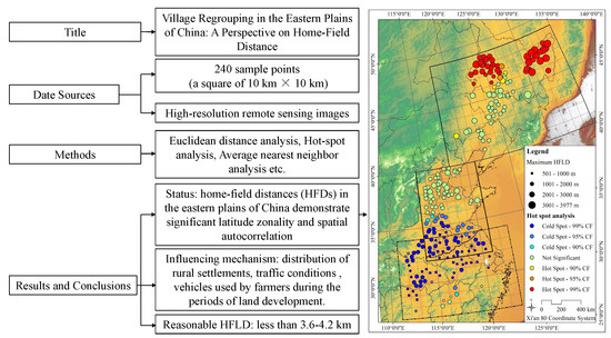
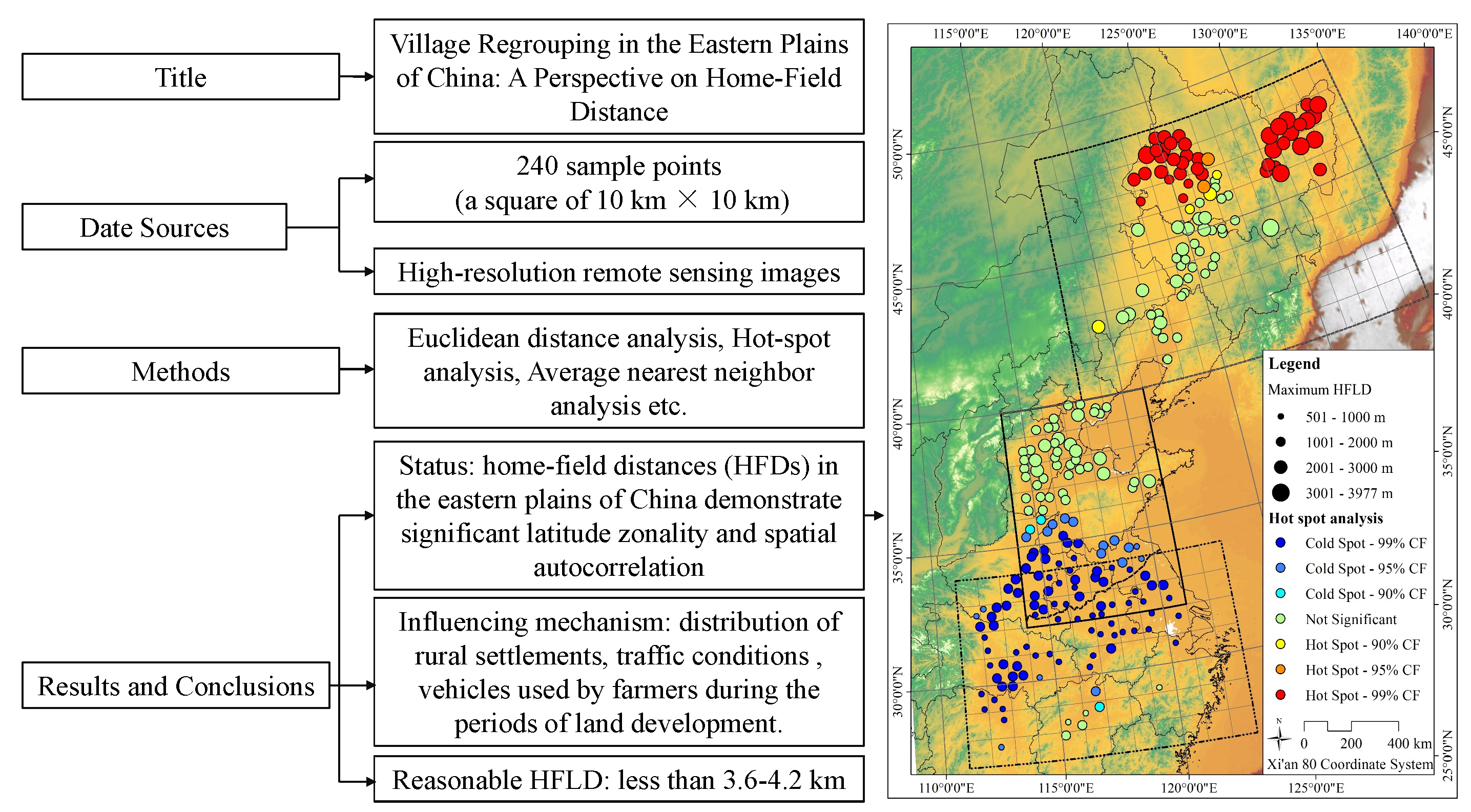
:Rural decline caused by rapid urbanization is a global issue, and village regrouping is an effective way to revitalize the countryside. The eastern plains of China (EPC) were the first regions to implement the policy of village regrouping in China. Despite being one of the most critical factors in village regrouping, home-field distances (HFDs) in these areas have received little attention. In this study, we selected 240 sample points in the EPC through spatial stratified sampling, each of which is a square of 10 × 10 km2. Based on high-resolution remote sensing images, the inter-regional differences of rural settlements and home-field straight-line distances (HFLDs) in the EPC were systematically analyzed. Based on the central place theory (CPT), the influencing mechanism of the HFLD, the maximum HFLD acceptable to farmers, and the reasonable number, distribution pattern, and service scope of central villages in the EPC were further explored. The results indicate that HFLDs in the EPC have significant latitude zonality and spatial autocorrelation. In the northeastern China plain (NECP), north China plain (NCP), and middle and lower reaches plain of the Yangtze River (MLPYR), the ranges of the maximum HFLD are 1000–4000 m, 500–2200 m, and 500–1500 m, respectively. The distribution pattern of rural settlements, the traffic conditions, and the vehicles used by farmers during periods of land development directly impact the HFLD. HFLDs in the EPC should not exceed 3.6–4.2 km (NECP can use the higher standard-4.2 km, NCP and MLPYR can use the lower standard-3.6 km), the service range of each rural settlement should not exceed 33.6–45.8 km2, and the number of rural settlements per 100 km2 should be greater than three. The rural settlements should be discretely distributed so that each piece of farmland can be tended. The MLPYR demonstrates the greatest potential for village regrouping, and the Chinese government should invest more funds in village regrouping and central village construction in the MLPYR. This study can provide a case study for developing countries in the urbanization phase, so as to improve the rationality of village regrouping planning.
1. Introduction
The rural decline caused by rapid urbanization is a global issue [1,2]. Developed countries in Europe and North America have encountered this problem in the last century and have taken measures to solve it. For developing countries in Asia and Africa, due to the late start of urbanization, the decline in rural areas has begun to emerge in recent decades [1,3]. Taking China as an example, since the economic reforms were launched, China’s urbanization rate has grown from 17.9% in 1978 to 57.35% in 2016, at an average annual rate of 1% [4]. Every year, hundreds of millions of peasant workers—most of whom are young and fit—leave their hometowns for cities, which has brought about a large number of inner decaying villages [1,5].
On the basis of the experiences of developed countries, village regrouping is an effective way to revitalize the countryside [3]. In 1947, the British government enacted the Town and Country Planning Act and began to implement a “key settlement policy” that divides all rural settlements into two categories: expandable and non-expandable. The government focused on the development of expandable rural settlements while limiting non-expandable rural settlements [6]. Japan has implemented a municipal, town, and village mergers and dissolutions policy for 120 years. In 1970, Japan enacted the Act on Special Measures for Promotion of Independence of Underpopulated Areas to promote the regrouping and revitalization of villages in underpopulated areas [7]. Some developing countries have also carried out similar rural development strategies. Nigeria proposed a village regrouping strategy in its second national development plan (1970–1974) [8]. Tanzania pursued a villagization program that reorganized scattered homesteads into nucleated villages in the mid-1970s [9]. Similar rural development strategies have been proposed by other African countries, such as Zambia and Malawi [10,11]. In general, the implementation of village regrouping policies in African countries is not due to rural hollowing, but to reduce infrastructure construction costs.
Village regrouping provides the necessary threshold population that makes the location of certain socio-economic facilities, markets, and services viable by gathering the scattered homesteads to form nucleated villages [8]. However, the village regrouping process usually leads to a sudden increase in the distances between homes and fields (home-field distances (HFDs)) [9,12]. Sudden changes in HFDs have a profound influence on socio-cultural and welfare conditions of farmers, and these changes may constrain agricultural productivity and community development [9,12,13,14,15]. A sudden increase in HFDs caused by village regrouping has the following negative effects. (1) Generally, an excessively long HFD has a negative influence on yields by poorer husbandry, such as less weeding, less careful harvests, and lower application of manure [12]; (2) A sudden increase in HFDs usually leads to a reduction in time for domestic life. Particularly for female farmers, they have less time available for child care, food storage and preparation, domestic cleaning, and carefully tending cooking fires [12,16]; (3) An excessively long HFD may cause previously cultivated areas to abandoned farmland and revert to scrub. The ownership of farmland far from the villages may be concentrated in the hands of wealthy farmers with tractors and pickup trucks [9,17]; (4) One solution to the problem of long HFDs is to establish on-field shelters. Especially during periods of high demand for labor, farmers can live in temporary shelters without having to make daily home-field visits. However, there are drawbacks for farmers who use temporary shelters in distant fields, as they are denied access to better living conditions and basic services during their absence from the village [9].
At the local scale, the impact of HFD changes caused by village regrouping has received widespread attention from different researchers [3,8,9,12,15,17]. However, there have been relatively few studies on the inter-regional differences of HFDs and the causes of such differences. A small number of studies have indicated that the agricultural mechanization level is the main factor affecting the HFD, so HFDs in contemporary agricultural areas are usually greater than HFDs in subsistence agricultural areas [3,15,17]. In addition, how to incorporate HFDs into regional village regrouping planning is a problem that needs to be further explored. The central place theory (CPT) can provide a theoretical basis for solving this problem. CPT was proposed by the German geographer Walter Christaller in 1933 to explain the number, size, and location of human settlements in a residential system. This theory is considered to be one of the most important discoveries of geography in the 20th century [18]. Christaller studied the settlement patterns in southern Germany and asserted that settlements simply functioned as “central places” providing services to their hinterlands. Christaller’s theory assumes that central places are distributed over an unbounded isotropic, homogeneous, limitless surface. Movement across the plane is uniformly easy in any direction, transportation costs vary linearly, and consumers act rationally to minimize transportation costs by visiting the nearest location offering the desired good or service [19]. The central place of different levels can supply particular types of service forming levels of hierarchy. Settlements that provide more goods and services than other places are called higher-order central places. Lower-order central places provide goods and services that are purchased more frequently than higher-order goods and services. Each central place has its limited service range and population threshold, which is determined by the maximum travel distance that consumers can accept to obtain the goods and services. Therefore, higher-order places are more widely distributed and fewer in number than lower-order places [20]. The service scope of each settlement is usually similar to a hexagonal lattice, as it is the most efficient pattern to serve areas without any overlap. Thus, Christaller used the concepts of “threshold” and “range” to provide a top-down explanation for the emergence of a cascading system of central places (Figure 1) [19].
Farming may be viewed as a system of movements articulated around rural settlements. Each rural settlement has its own farming radius, and the farming radius is determined by the maximum home-field straight-line distance (HFLD) acceptable to farmers. The farming radius further determines the number and distribution of rural settlements. Therefore, according to the central theory, at the regional scale, village regrouping planning needs to address the following four issues about HFDs: (1) inter-regional differences of HFDs; (2) the influencing mechanism of such differences; (3) the maximum HFD acceptable to farmers in these regions; (4) the number, distribution pattern, and service scope of rural settlements to meet the farmers’ requirements for HFDs.
China is the largest developing country in the world. In 2017, the Chinese government began to implement a rural revitalization strategy, and village regrouping was chosen as an important means to promote the reconstruction of rural areas. The eastern plains of China (EPC) are the most developed and densely populated areas in China. The EPC are also one of the regions with a high level of land fragmentation and hollowing of rural settlements in China [21]. Moreover, the EPC were the first regions to implement the village regrouping policy in China. Shandong Province, located in the north China plain (NCP), has been implementing a pilot project of village regrouping since 2006. Despite being one of the most critical factors for village regrouping, HFDs in these areas have received little attention. Only a few studies have been conducted on a local scale. Hu Sun et al. investigated the maximum home-field straight-line distances (HFLDs) acceptable to farmers in Yucheng County, Shandong Province, China. The results showed that the maximum HFLDs acceptable to farmers were quite different (57% less than 1 km, 18% within 1–1.5 km, 24% greater than 1.5 km) [3]. Lijing Tang et al. analyzed the reasonable HFLDs of Yiyuan County in Shandong Province by establishing an HFLD calculation model. In this study, the weighted average speed of various types of vehicles used by farmers was used as a criterion for calculating the maximum HFLD. The results showed that the maximum HFLD in this area should not exceed 3.2 km [22].
In this study, we selected 240 sample points in the EPC through spatial stratified sampling, each of which is a square of 10 km × 10 km. Based on high-resolution remote sensing images, the inter-regional differences of rural settlements and HFLDs in the EPC were systematically analyzed through Euclidean distance analysis, hot spot analysis, and average nearest neighbor analysis. Moreover, the influencing mechanism of HFLD, the maximum HFLD acceptable to farmers, and the reasonable number, distribution pattern, and service scope of rural settlements in the EPC were further explored.
2. Materials and Methods
2.1. Study Area
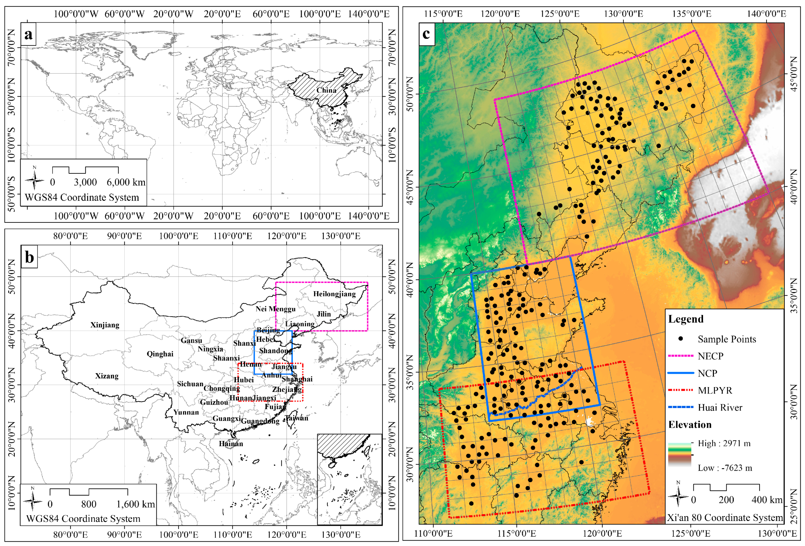
The EPC consist of the northeast China plain (NECP), the NCP, and the middle and lower reaches plain of Yangtze River (MLPYR) (Figure 2). The NECP is the largest plain in China, with a total area of approximately 35 × 105 km2 (longitude 40°–48° N and latitude 118°–135° E). The NECP belongs to the continental monsoon climate. The average annual temperature is between −3 and 11 °C, and the accumulated temperature ≥10 °C is 2200–3600 °C. The average rainfall is 350–700 mm, mainly concentrated in July to September. The two main types of soil are black and chernozem, which are fertile and have strong water-holding capacities. The main crops in the NECP include rice, soybean, and maize [23].
The NCP is China’s second largest plain, with a total area of approximately 30 × 105 km2 (longitude 32°–40° N and latitude 114°–121° E). NCP is one of the most densely populated regions in the world. It is also the political and cultural center of China, and the national capital city (Beijing) is located at its northeast edge. The NCP is located in the warm temperate monsoon climate zone, and the four seasons change significantly. The average annual temperature is between 8 to 15 °C, and the accumulated temperature ≥10 °C is 3800–4900 °C. The average rainfall is 500–900 mm, mainly concentrated in July to September. The NCP is a high-yield agricultural area, and the main cropping system is a winter wheat-summer maize double-cropping rotation [24].
The MLPYR is the third largest plain in China, with a total area of approximately 20 × 105 km2 (longitude 27°–34° N and latitude 111°–123° E). The MLPYR belongs to the subtropical monsoon climate. The average annual temperature is between 14 to 18 °C, and the accumulated temperature ≥10 °C is 4500–6500 °C. The average rainfall is 800–1400 mm. Monsoon activities transport a very large amount of atmospheric moisture from the East and the South China Sea to the MLPYR, which is the region with the highest density of water networks in China. The main crop in the MLPYR is rice, and the rice planting area accounts for approximately 78% of the total crop area in the MLPYR. The NCP and MLPYR have some overlap in latitude, and the Huaihe River is the dividing line between them [25,26].
2.2. Data Sources and Methods
In this study, we selected a total of 240 sample points in the EPC (NECP-88; NCP-88; and MLPYR-64) through spatial stratified sampling. Each sample point was a square of 10 km × 10 km (Figure 2; Figure 3). First, the study area was divided into 1° × 1° (unit: longitude and latitude) grids (Figure 2c). Then, the number of sample points in each grid was determined based on the percentage of areas where the slope was less than 6° (≥70%, 3; 40–70%, 2; ≤40%, 1 or not).
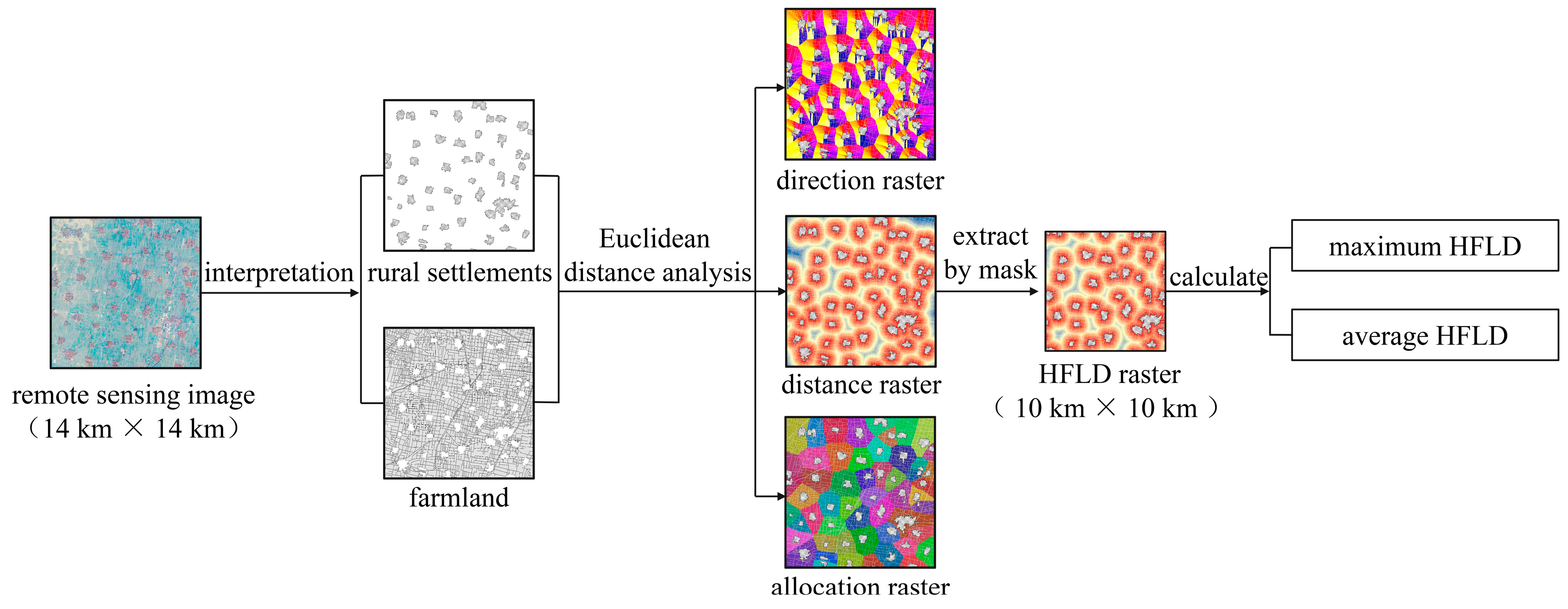
The detailed calculation process of HFLDs in each sample point is as follows (Figure 3). (1) Extract the remote sensing image of each sample point by GIS (resolution, 1.85 m; coordinate system, Xi’an 80; time, 2017). The range of the remote sensing image was extended to 14 km × 14 km to ensure that each farmland can find its nearest rural settlement; (2) Extract the patches of rural settlements and farmland through visual interpretation. It was found through pre-experiment that interpretation software, such as Envi and Erdas, could not accurately distinguish farmland and rural settlement patches from other types of patches, such as grassland and road. Therefore, in order to increase the accuracy of interpretation, this study used a manual visual interpretation method. First, the remote sensing image of each sample point was imported into ArcGIS 10.2, and two shapefiles were created to vectorize the patches of farmland and rural settlements. In the process of vectorization, different people adopted a common interpretation standard (same coordinate system, code, etc.); (3) Calculate the straight-line distance from each farmland to its nearest rural settlement by the Euclidean distance analysis tool in ArcGIS 10.2. HFD can be divided into two types: HFLD and home-field path distance (HFPD). HFPD is more in line with farmers’ travel modes. HFLD makes it easier for planners to determine the service radius of each village. HFLD and HFPD can be calculated using the Euclidean distance tool and network analysis tool in ArcGIS, respectively. Since the calculation of HFPD requires the vectorization of roads, its calculation process is more complicated. From the perspective of serving the planner, and for the convenience of calculation, the Euclidean distance tool in ArcGIS 10.2 was used to analyze the HFLDs in the EPC; (4) Calculate the maximum HFLD and average HFLD at different sample points; (5) Identify whether the HFLDs in the EPC have global spatial autocorrelation, local spatial autocorrelation, and latitude zonality through spatial autocorrelation analysis, hotspot analysis, and correlation analysis, respectively; (6) Calculate the number, size, and distribution pattern of rural settlements at each sample point. The analysis methods used in this study were as follows.
2.2.1. Euclidean Distance Analysis
The Euclidean distance refers to the straight-line distance between two points in n-space [27,28]. The Euclidean distance used in HFLD analysis refers to the straight-line distance between farmland and its nearest rural settlement. The Euclidean distance analysis tool in ArcGIS 10.2 can be used to calculate the straight-line distance from the center of the source grid to the center of each surrounding grid [29]. In HFLD analysis, source grids and surrounding grids refer to rural settlements and farmland, respectively. The results of Euclidean distance analysis include Euclidean direction raster, Euclidean distance raster, and Euclidean allocation raster. The Euclidean direction raster contains the azimuth direction from each farmland to the nearest rural settlements. The Euclidean distance raster contains the straight-line distance from each farmland to its nearest rural settlements. Each grid in the Euclidean allocation raster is assigned the values of the rural settlements to which it is closest, as determined by the Euclidean distance algorithm (Figure 3).
2.2.2. Spatial Autocorrelation Analysis
The spatial autocorrelation tool in ArcGIS 10.2 was used to analyze whether the maximum and average HFLDs in the EPC showed global spatial autocorrelation. This tool evaluates the spatial autocorrelation by calculating the Moran’s I value, and further indicates the significance of the index by Z-values and P-values [30]. In general, the Global Moran’s Index is bounded by −1.0 and 1.0. A positive Moran’s I index value exhibits a tendency towards clustering (high values cluster near other high values, and low values cluster near other low values). A negative Moran’s I index value demonstrates a tendency towards dispersion (high values tend to be close to low values and repel other high values) [31]. If the Z-score is less than −2.58 or greater than +2.58 and the P-value is less than 0.01, then the confidence level (CF) is 99%. If the Z-score is less than −1.96 or greater than +1.96 and the P-value is less than 0.05, then the CF is 95% [32].
The Global Moran’s I index for spatial autocorrelation is given as (Equations (1) and (2)):
where is the deviation of an attribute (maximum and average HFLD) for sample point from its mean (); is the spatial weight between sample points and ; is equal to the total number of sample points; and is the aggregate of all the spatial weights. is determined by the distance between points and . Nearby neighboring points have a larger spatial weight on the computations for a target point than points that are far away (the nearest point has a spatial weight of 1, and the farthest point has a spatial weight of 0).
2.2.3. Hot Spot Analysis
The hot spot analysis tool in ArcGIS 10.2 was used to analyze whether the maximum and average HFLDs in the EPC showed a local spatial autocorrelation, as well as areas with high-value clustering or low-value clustering. In general, a sample point with a high/low value is not a statistically significant hot/cold spot. However, if it’s surrounding sample points also have high/low values, then this sample points can be identified as a statistically significant hot/cold spot [33,34]. The hotspot analysis tool calculates the local sum of a sample point and its adjacent sample points and then compares the calculation result with the sum of all the sample points. When the local sum is obviously different from the expected local sum, it is not a random result and produces a statistically significant Z-score. This tool calculates the Getis-Ord Gi* statistic for each sample points and the Getis-Ord Gi* statistic returned for each sample point is assigned to be a Z-score. For a statistically significant positive Z-score, the larger the Z-score is, the more intense is the clustering of high values (hot spot). For a statistically significant negative Z-score, the smaller the Z-score is, the more intense is the clustering of low values (cold spot) [35,36,37].
The Getis-Ord Gi* is given as Equations (3)–(5):
where is the attribute value for feature ; is the spatial weight between feature and (same as spatial autocorrelation analysis); and is equal to the total number of sample points.
2.2.4. Average Nearest Neighbor Analysis
The average nearest neighbor analysis measures the average distance between each rural settlement and its nearest neighbors. If the average distance is less than the average for a hypothetical random distribution, the distribution of the rural settlements being analyzed is considered to be clustered. If the average distance is greater than that of a hypothetical random distribution, the distribution of rural settlements is considered to be dispersed [38]. The average nearest neighbor index () can be used to identify whether the distribution of rural settlements is clustered or dispersed, and Equations (6)–(8) can be used for its calculation:
where is the observed mean distance between each rural settlement and its nearest neighbor; is the expected mean distance for rural settlements given in a random pattern; is equal to the distance between rural settlement and its nearest neighbor. is the area of the minimum enclosing rectangle around all rural settlements and represents the total number of rural settlements. The average nearest neighbor tool can initiate five values: observed mean distance, expected mean distance, nearest neighbor index, Z-score, and P-value. If ANN is less than 1, the distribution of rural settlements in the study area is towards clustering. If ANN is greater than 1, the trend is towards scattered distribution. If the Z-score is less than −2.58 or greater than +2.58 and the P-value is less than 0.01, then the CF is 99%. If the Z-score is less than −1.96 or greater than +1.96 and the P-value is less than 0.05, then the CF is 95%.
2.2.5. Method of Calculating the Maximum HFLD Acceptable to Farmers
The suitable maximum HFLD in a certain area is affected by the commuting time acceptable to farmers, the transport modes used by farmers, and the conversion coefficient between the HFLD and HFPD [17]. The maximum HFLD is given as Equation (9):
where R is the maximum HFLD, m; V is the speed of vehicles used by the farmers when the field is far away and goods need to be transported, m/min; T is the longest commuting time acceptable to farmers, min; and k is the non-linear coefficient of the road network (HFPD/HFLD, dimensionless).
2.2.6. Calculation Method of the Maximum Service Scope and Number of Rural Settlements
According to CPT [18], the service scope of each settlement is usually similar to a regular hexagon, so the maximum service scope and number of rural settlements are given as (Equations (10) and (11)):
where S is the maximum service range of each rural settlement, km2; R is the maximum HFLD, m; and N is the number of rural settlements per 100 km2.
2.2.7. Historical Analysis of Land Development in the EPC
The formation of the distribution patterns of HFLDs and rural settlements is a long-term historical process. Thus, to illustrate the influencing mechanism of spatial differences of HFLDs and rural settlements in the EPC, the land development history in the EPC was analyzed.
3. Results
3.1. Distribution Pattern of HFLDs and Rural Settlements in the EPC
3.1.1. HFLDs in the EPC Demonstrate Significant Latitude Zonality
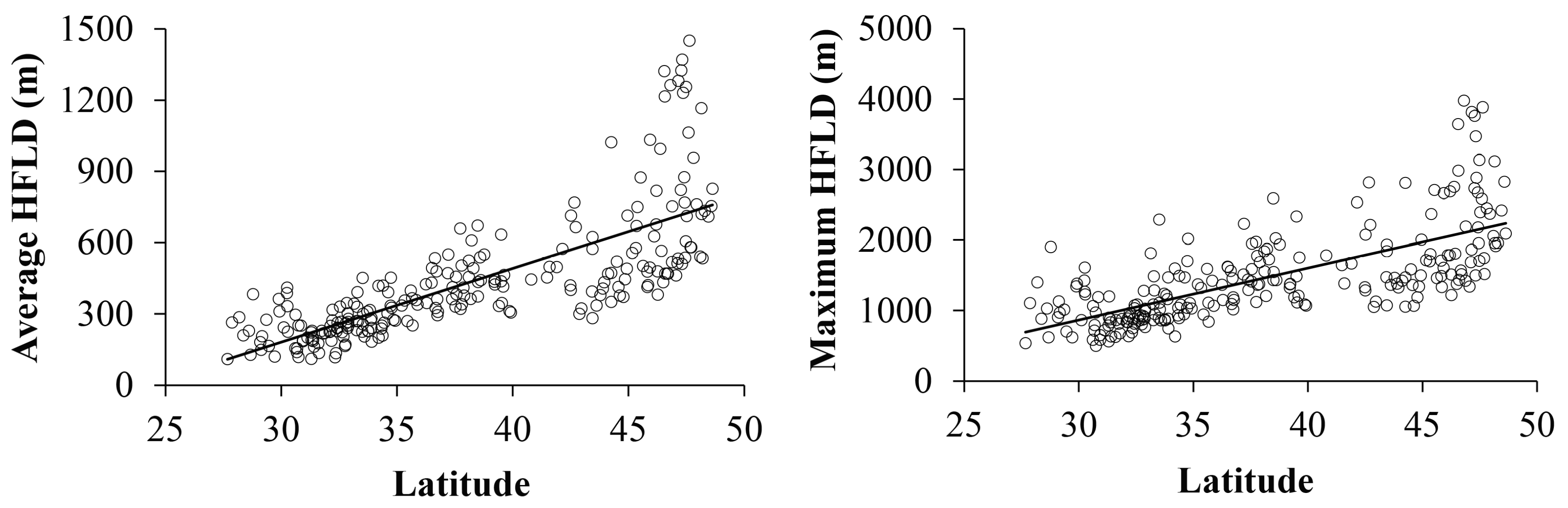
The results of Euclidean distance analysis show that the maximum and average HFLDs in EPC are less than 4000 m and 1500 m, respectively. Both the maximum and average HFLDs demonstrate a significant positive correlation with latitude (Figure 4). In the NECP area, the range of maximum and average HFLDs are 1000–4000 m and 400–1050 m, respectively. Approximately 80.3% of farmland is located within 1000 m of the nearest rural settlement, and 2.7% of farmland is located more than 2000 m away. In the NCP area, the ranges of the maximum HFLD and the average HFLD are 500–2200 m and 250–500 m, respectively. Approximately 96.6% of farmland is located less than 1000 m away from the nearest rural settlement, and only 0.1% of farmland is located more than 2000 m away. The ranges of maximum and average HFLDs are 500–1500 m and 100–400 m, respectively in the MLPYR, and 99.6% of farmland is located less than 1000 m away from the nearest rural settlement (Figure 5, Table 1).
3.1.2. HFLDs in the EPC Demonstrate Significant Spatial Autocorrelation
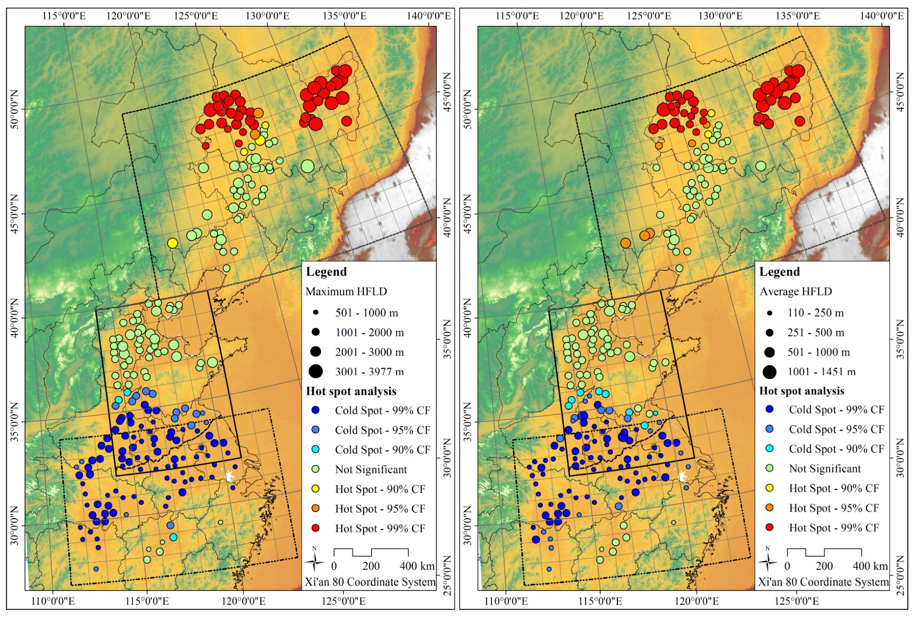
The spatial autocorrelation analysis result for the average HFLD illustrates that the Global Moran’s I index is 0.663980; the Z-score is 28.27; and the P-value <0.01. The spatial autocorrelation analysis result for the maximum HFLD demonstrates that the Global Moran’s I index is 0.577916; Z-score is 24.57; and P-value <0.01. The average and maximum HFLDs in the EPC exhibit significant spatial autocorrelation. The results of hot spot analysis indicate that the hot spot area with CF greater than 99% is mainly located in the northern area of the NECP, and the cold spot area with CF greater than 99% is mainly located in the southern area of the NCP and the northern area of the MLPYR (Figure 6).
3.1.3. Rural Settlements in the EPC Present Significant Spatial Differences
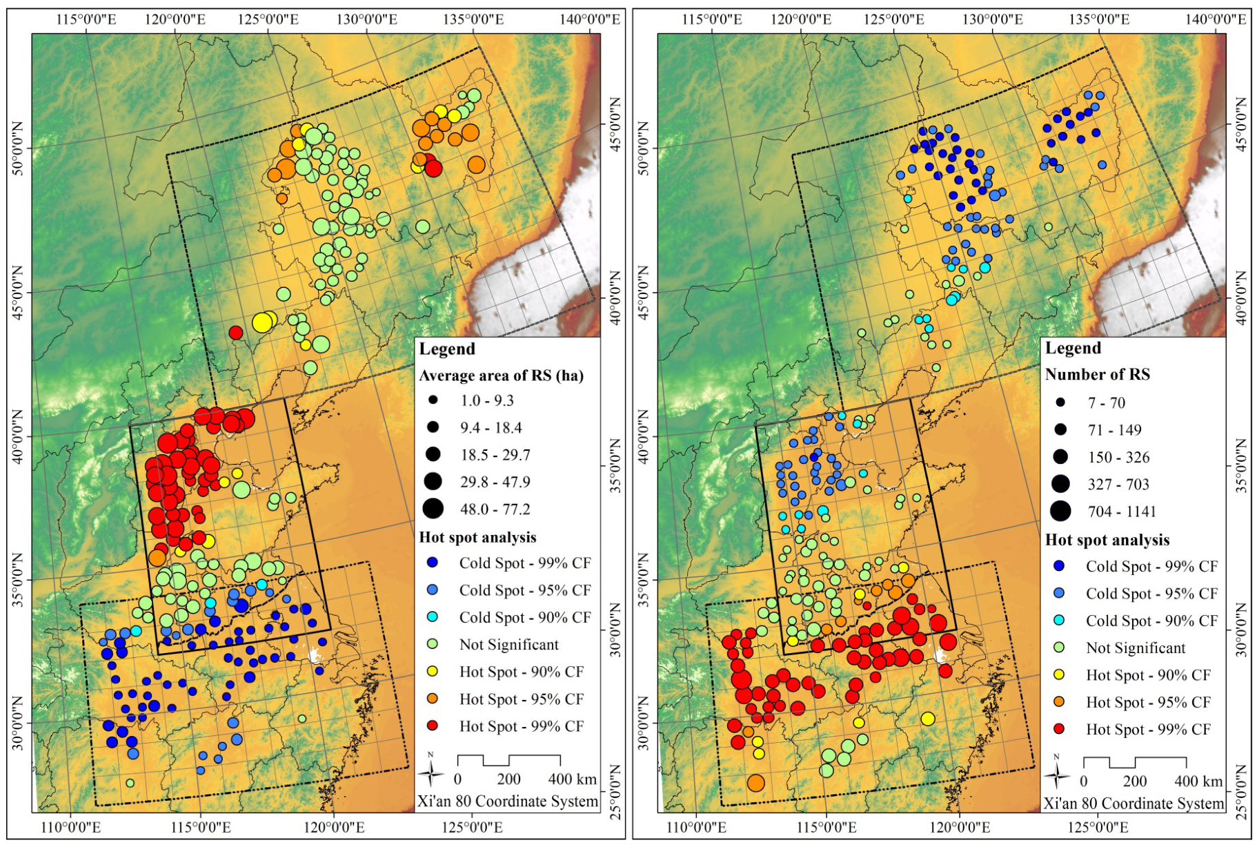
The average patch number of rural settlements in the NECP, NCP, and MLPYR is 34.8, 69.1, and 214.4 per 100 km2, respectively. The average patch area of rural settlements in the NECP, NCP, and MLPYR is 21.4, 25.5, and 7.0 hm2 per 100 km2, respectively (Figure 7). The results of hot spot analysis indicate that the central and southern parts of the MLPYR demonstrate the largest average patch number and smallest patch area of rural settlements, illustrating that this area has the highest fragmentation level of rural settlements. In addition, the regions with the largest average patch area of rural settlements are located in the northern parts of the NCP (99% CF) and NECP (95% CF); the areas with the smallest average patch number are also located in the northern parts of the NCP (95% CF) and the NECP (99% CF), demonstrating that these areas have the lowest fragmentation levels of rural settlements (Figure 8).
3.1.4. Rural Settlements in the EPC Demonstrate a Discrete Distribution
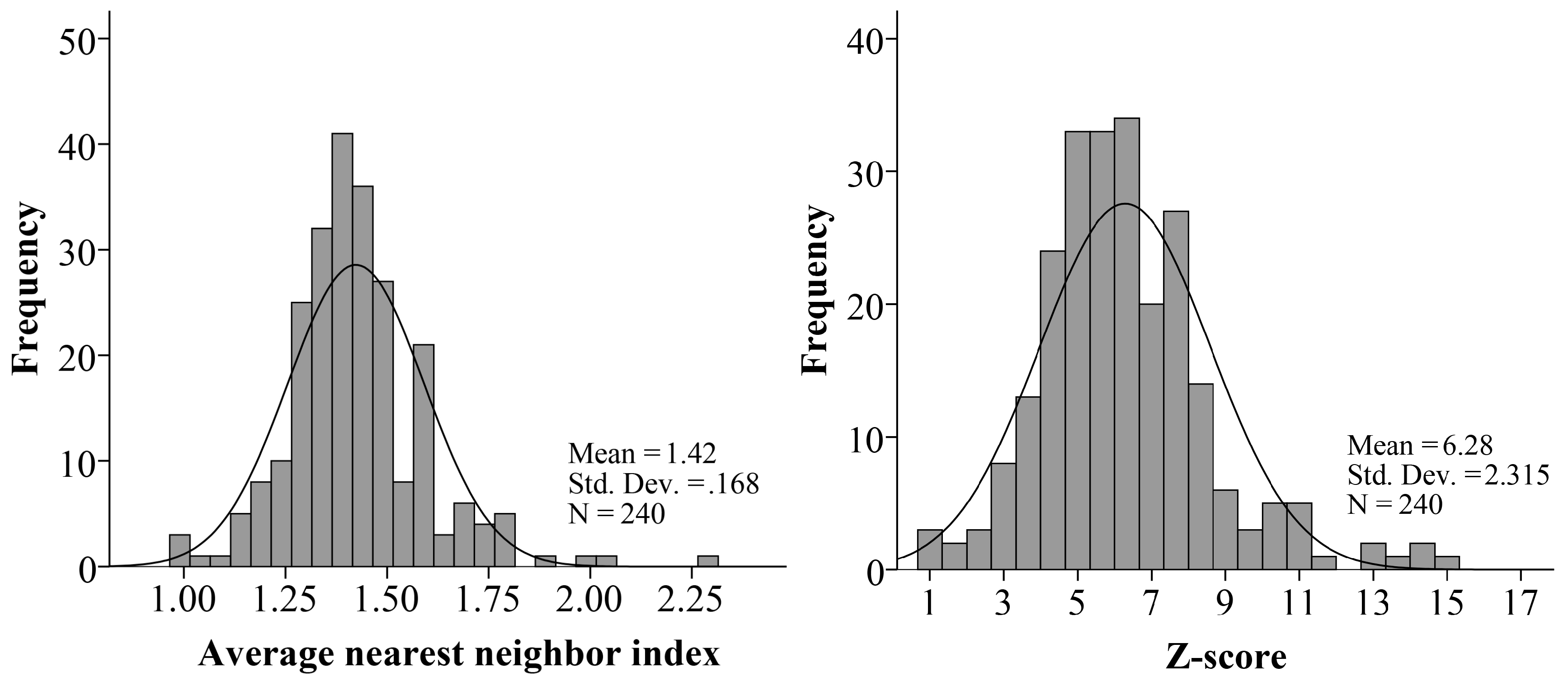
The results of the average nearest neighbor analysis indicate that more than 95% of the sample points exhibit an greater than 1; Z-score greater than 2.58; and P-value less than 0.01, illustrating that rural settlements are usually discretely distributed in the EPC (Figure 9).
3.2. Mechanism of North-South Differences of HFLDs and Rural Settlements
The northern part of the NECP is called the “Great Northern Wilderness”. During the Qing Dynasty (1636–1912), the Qing government forbade Han people to access the NECP area, and this action made the “Great Northern Wilderness” sparsely populated. In the 1950s, the “Great Northern Wilderness” witnessed a period of large-scale development as thousands of demobilized soldiers, intellectual youth, and revolutionary cadres responded to the call of the country and established a large number of state-owned and military farms. This area is flat, fertile, and sparsely populated. At the beginning of land development, tractors were the main tillage and transportation tools. Therefore, this area demonstrates the greatest HFLD and the lowest density of rural settlements in the EPC [39,40,41].
Land development occurred relatively early in the southern part of the NECP. Between 1653 and 1668, the Qing government encouraged people to carry out land development, and the development area was mainly located in Liaoning Province (Figure 2). Although the Qing government banned the development of the NECP after 1668, the farmland area in Liaoning Province has continued to increase significantly. In contrast, during the same period in Jilin and Heilongjiang Provinces (Figure 2), only local development was carried out, resulting in a desolate scene overall. The Qing government’s ban on the NECP has undergone a gradual release process, from the partial opening in 1860 to the full opening after the Sino-Japanese War (1894–1895). Then, large-scale land development began in the Liaoning, Jilin, and the southern part of Heilongjiang Provinces, and gradually pushed from the south to the north. By the end of the Qing Dynasty, land development in the southern part of the NECP had nearly completed, and the distribution pattern of farmland and rural settlements had basically taken shape [39,40,41].
The NCP belongs to the warm temperate monsoon climate, and the four seasons change significantly so that this area is suitable for living. The main soil in the NCP is loess, so crops survive easily, and weeds are easy to remove. Before the Song Dynasty, the NCP was one of the most developed agricultural areas in China. Due to frequent wars, natural disasters, and ecological destruction during the Song (960–1279), Jin (1115–1234), and Yuan (1271–1368) Dynasties, agriculture severely declined in the NCP. On this basis, agriculture in the NCP experienced restoration and development during the Ming Dynasty (1368–1644). In the Qing Dynasty, the NCP developed into an important food production area in China [39,41,42]. Therefore, the pattern of farmland and rural settlements in the NCP basically took shape during the Ming and Qing dynasties. At that time, walking, carriages, and carts were the main ways for farmers to travel in the NCP and the southern part of the NECP. The farmers had a limited tillage range, and the maximum HFLD was usually 1–2 km. On the other hand, the NCP is a semi-arid climate zone. There are few rivers, and the groundwater level is generally deep. Wells cannot be drilled everywhere, and dispersed living is not conducive to fetching water at a fixed location. Therefore, rural settlements in the NCP demonstrate a lower fragmentation level [39].
China’s economic center gradually moved from the NCP to the MLPYR after the Tang Dynasty (618–907). Until the Southern Song Dynasty (1127–1279), the economic development of the MLPYR significantly exceeded that of the NCP. The Yangtze River basin was further developed during the Ming and Qing dynasties, and the land development in the MLPYR was basically completed. Furthermore, due to the low-lying terrain, dense river network, and high viscosity soil, a network of transportation roads was difficult to establish. Farmers had to rely on water systems to build a scattered distribution pattern of rural settlements during the land development process in the MLPYR. As the main mode of transportation, ship, is slow, it made the farmers’ travel range relatively limited [39,43,44]. Therefore, HFLDs in the MLPYR are shorter than those in the NCP and NECP.
From the perspective of the land development history in the EPC, the distribution pattern of rural settlements, the traffic conditions, and the vehicles used by farmers during periods of farmland development directly impact the HFLD. Climate, soil, policies, and other factors have an indirect impact on the HFLD by affecting the traffic conditions and the distribution of rural settlements.
3.3. Maximum HFLD Acceptable in the EPC
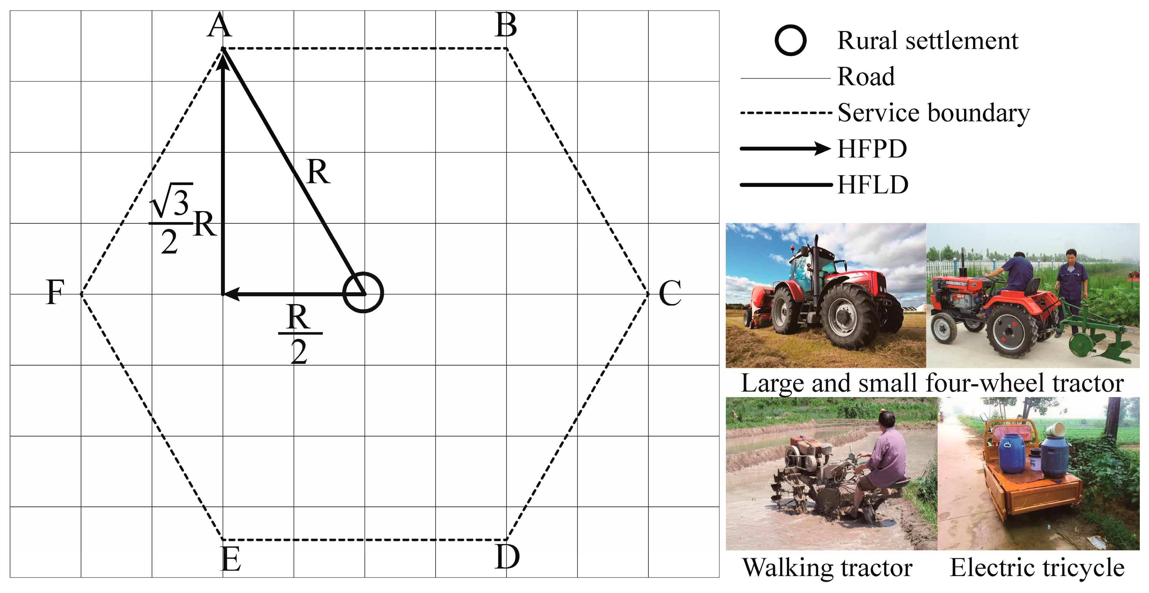
The maximum commuting time per trip acceptable to farmers in the EPC usually does not exceed 20 min [45,46]. In the EPC, alternative travel modes for farmers include large and medium tractor, small tractor, walking tractor, motorcycle, electric tricycle, electric bicycles, tricycle, bicycle, and walking [45,46,47]. When a field is far away and goods need to be transported, farmers often choose the tractor and electric tricycle as their transport modes (sowing or harvesting season-tractor; daily transportation-electric tricycle) [48]. The speed of an electric tricycle is generally higher than that of a tractor. Therefore, the speed of a tractor was used as the standard for calculating the maximum HFLD in the EPC, and this standard can also meet the needs of electric tricycle users. The average speed of a tractor on rural roads is 15 km/h [46].
As shown in Figure 10, the road network in the EPC is usually grid-shaped, and points A, B, E, and D have the longest HFLD and HFPD values. HFPD/HFLD is equal to 1.366. However, the road network in the EPC is not a standard grid network, and the range of the non-linear coefficient is 1.2–1.4 [43]. Therefore, we selected a non-linear coefficient equal to 1.2 and 1.4, respectively, to calculate the range of the suitable maximum HFLD in the EPC. The results prove that HFLDs in the EPC should not exceed 3.6–4.2 km. The maximum HFLD exceeds 4 km in some parts of the NECP, so the suitable maximum HFLD in the NECP can use the higher standard (4.2 km). The current maximum HFLDs in the NCP and MLPYR are 2200 m and 1500 m, respectively. Therefore, these two regions can use the lower standard (3.6 km).
3.4. Number, Distribution Pattern, and Service Scope of Rural Settlements
The results indicate that the service range of each village should not exceed 33.6–45.8 km2, and the number of villages per 100 km2 should be greater than three. To ensure that each piece of farmland can be tended, the rural settlements should be discretely distributed after village regrouping. The HFLDs and the service ranges of rural settlements in different regions can be reduced according to the population and traffic conditions; at the same time, the number of rural settlements should be increased.
4. Discussion
4.1. Comparison of This Study with Similar Studies
The northern part of the NECP is the largest contemporary agricultural region and the region with the highest level of agricultural mechanization in the EPC. This region also has the largest HFLD in the EPC. Therefore, the distribution characteristic of HFDs in the EPC is consistent with related studies (“HFDs in contemporary agricultural areas are usually greater than HFDs in subsistence agricultural areas”) [3,15,17]. However, in our opinion, the formation of the distribution pattern of HFLDs is a long-term historical process. Therefore, in areas where large-scale village regrouping has not yet taken place, the current agricultural mechanization level is not the major factor. From the perspective of the land development history in the EPC, the distribution pattern of rural settlements, the traffic conditions, and the vehicles used by farmers during periods of farmland development directly impact the HFLD.
There are two methods for determining the maximum HFD acceptable to farmers: the questionnaire method and the model calculation method. If we directly investigate the maximum HFD acceptable to farmers, the survey results of different farmers are quite different as farmers cannot accurately understand the concept of the HFD [3]. However, their comprehension of commuting time is much more accurate. Therefore, it is more reasonable to calculate the maximum HFD acceptable to farmers by investigating the maximum commuting time acceptable to farmers and the speed of the vehicles used by the farmers. In addition, farmers usually use a variety of vehicles. Therefore, another issue is which vehicle to choose as the standard for calculating the suitable maximum HFD. Unlike related studies (“the weighted average speed of various types of vehicles used by farmers was used as a criterion for calculating the maximum HFD”) [22], in this study, the vehicles used by farmers when a field is far away and goods need to be transported were selected as the calculation standard for the maximum to ensure that the commuting needs of farmers can be met under any condition.
4.2. Implications for Policy-Making of Village Regrouping
The basic principle of village regrouping is defined as “promote small and micro rural settlements gathering to large and medium-sized rural settlements with good infrastructure and convenient transportation; at the same time, keep the HFDs within an acceptable range” [17]. Therefore, village regrouping has great potential in a specified area if the fragmentation level of rural settlements is relatively high and the current HFLDs are relatively short. The MLPYR exhibits the highest fragmentation level of rural settlements and the shortest HFLDs; the NECP demonstrates the lowest fragmentation level of rural settlements and the longest HFLDs. It is clear that these two areas have the greatest and least potential for village regrouping, respectively. Therefore, the Chinese government should invest more funds in village regrouping and central village construction in the MLPYR. In addition, rural development policy makers and rural planners in the EPC should prepare guidelines for village regrouping planning that include the following items: current HFDs in different regions; maximum HFD acceptable to farmers; the appropriate number, distribution pattern, and service scope of rural settlements in different regions.
4.3. Limitations and Prospects of This Study
This study can provide a case study for developing countries in the urbanization phase to improve the rationality of village regrouping planning at the regional scale. However, this study has the following deficiencies: (1) Considering that the administrative boundaries of villages need to be re-delineated after village regrouping, the influence of administrative boundaries is neglected in the calculation of HFLDs; (2) The maximum HFLD acceptable to farmers calculated in this study is a theoretical maximum value, and no specific HFLD is proposed for the actual traffic conditions in different regions; (3) The calculation of village regrouping potential in different regions needs to comprehensively consider topography and landforms, traffic conditions, distribution of farmland, administrative boundaries, inter-regional economic and cultural differences, and other factors. This article only provides a qualitative analysis from the perspective of the HFLD and does not consider other factors. Therefore, follow-up studies need to consider a variety of factors to explore the suitable maximum HFLD and village regrouping potential in different regions.
5. Conclusions
HFLDs in the EPC demonstrate significant latitude zonality (NECP > NCP > MLPYR) and spatial autocorrelation. In the NECP, NCP, and MLPYR, the ranges of the maximum HFLD are 1000–4000 m, 500–2200 m, and 500–1500 m, respectively. The distribution pattern of rural settlements, the traffic conditions, and the vehicles used by farmers during the periods of farmland development directly impact the HFLDs in the EPC. Climate, soil, policies, and other factors have an indirect impact on the HFLDs by affecting the traffic conditions and the distribution of rural settlements.
HFLDs in the EPC should not exceed 3.6–4.2 km (NECP can use the higher standard-4.2 km, NCP and MLPYR can use the lower standard-3.6 km). The service range of each village should not exceed 33.6–45.8 km2, and the number of villages per 100 km2 should be greater than three. The rural settlements should be discretely distributed after village regrouping so that each piece of farmland can be tended. The MLPYR demonstrates the greatest potential for village regrouping, and the Chinese government should invest more funds in village regrouping and central village construction in the MLPYR. This study can provide a case study for developing countries in the urbanization phase, so as to improve the rationality of village regrouping planning.
Author Contributions
X.L., Y.L., Y.C., P.L., and Z.Y. conceived, designed, prepared, and revised the paper together. All authors read and approved the final manuscript.
Funding
This research was funded by the National Science and Technology Support Plan of China (Project Number: 2012BAJ24B05). And the APC was funded by the project on restoration of ecological service and landscape in rural land consolidation supported by the Ministry of Natural Resources of China.
Conflicts of Interest
The authors declare no conflicts of interest. The funding sponsors had no role in the design of the study, the collection, analyses or interpretation of data, the writing of the manuscript, nor in the decision to publish the results.
References
- Liu, Y.S.; Li, Y.H. Revitalize the world’s countryside. Nature 2017, 548, 275–277. [Google Scholar] [CrossRef] [PubMed] [Green Version]
- Elshof, H.; Haartsen, T.; van Wissen, L.J.G.; Mulder, C.H. The influence of village attractiveness on flows of movers in a declining rural region. J. Rural Stud. 2017, 56, 39–52. [Google Scholar] [CrossRef]
- Sun, H.; Liu, Y.S.; Xu, K.S. Hollow villages and rural restructuring in major rural regions of China: A case study of Yucheng City, Shandong Province. Chin. Geogr. Sci. 2011, 21, 354–363. [Google Scholar] [CrossRef] [Green Version]
- Liu, Y.; Cheng, S.K.; Ge, Q.S.; Yu, G.R. China Statistical Yearbook (2017); China Statistics Press: Beijing, China, 2017. [Google Scholar]
- Liu, Z.; Liu, S.H.; Jin, H.R.; Qi, W. Rural population change in China: Spatial differences, driving forces and policy implications. J. Rural Stud. 2017, 51, 189–197. [Google Scholar] [CrossRef]
- Smith, S.A. Town and Country Planning Act, 1947. Mod. Law Rev. 1948, 11, 72–81. [Google Scholar]
- Traphagan, J.W. Demographic Change and the Family in Japan’s Aging Society; State University of New York Press: New York, NY, USA, 2003. [Google Scholar]
- Saleh, A. Concept of village regrouping as an alternative strategy for sustainable micro regional development. In Urban Planning and Architectural Design for Sustainable Development; Naselli, F., Pollice, F., Amer, M.S., Eds.; Springer: Berlin, Germany, 2016; Volume 216, pp. 933–937. [Google Scholar]
- Sokoni, C.H. Home to field distance in western Bagamoyo, Tanzania: Lessons for rural development policy and practice. Utafiti 2011, 2, 86–98. [Google Scholar]
- Pius, N. State power, land-use planning, and local responses in Northwestern Zimbabwe, 1980s–1990s. Afr. Stud. Q. 2014, 14, 37–60. [Google Scholar]
- Happy, M.K. Malawi’s economic and development policy choices from 1964 to 1980: An epitome of ‘Pragmatic Unilateral Capitalism’. Nord. J. Afr. Stud. 2011, 2, 112–131. [Google Scholar]
- Macall, M.K. The significance of distance constraints in peasant farming systems with special reference to sub-Saharan Africa. Appl. Geogr. 1985, 4, 325–345. [Google Scholar] [CrossRef]
- Kassali, R.; Ayanwale, A.B.; Williams, S.B. Farm location and determinants of agricultural productivity in the Oke-Ogun Area of Oyo State, Nigeria. J. Sustain. Dev. Afr. 2009, 2, 1–19. [Google Scholar]
- Williams, T.O. Factors influencing manure application by farmers in semi-arid west Africa. Nutr. Cycl. Agroecosyst. 1999, 1, 15–22. [Google Scholar] [CrossRef]
- Liu, L. Labor location and agricultural land use in Jilin, China. Prof. Geogr. 2000, 1, 74–83. [Google Scholar] [CrossRef]
- Ganapathy, R.S. The political economy of rural energy planning in the third world. Rev. Radic. Political Economics 1983, 3, 83–95. [Google Scholar] [CrossRef]
- Li, X.D.; Yang, Y.; Yang, B.; Zhao, T.; Yu, Z.R. Layout optimization of rural settlements in mountainous areas based on farming radius analysis. Trans. Chin. Soc. Agric. Eng. 2018, 12, 267–273. [Google Scholar] [CrossRef]
- Berry, B.J.L.; Garrison, W.L. Recent developments of central place theory. Papers Reg. Sci. 2010, 4, 107–120. [Google Scholar] [CrossRef]
- Mulligan, G.F. Central place theory and its reemergence in regional science. Ann. Reg. Sci. 2012, 48, 405–431. [Google Scholar] [CrossRef]
- Hsu, W.T. Central Place Theory and City Size Distribution. Econ. J. 2012, 122, 903–932. [Google Scholar] [CrossRef]
- Liu, Y.S.; Long, H.L.; Chen, Y.F.; Wang, J.Y. China ‘s Rural Development Research Report: Rural Hollowing and Consolidation Strategy; China Science Press: Beijing, China, 2011. [Google Scholar]
- Tang, L.J.; Wang, D.Y.; Wang, L.L. Rational distribution of rural settlements based on farming radius: A case study in rural-urban construction land in Yiyuan County, Shandong Province. China Popul. Resour. Environ. 2014, 6, 59–64. [Google Scholar] [CrossRef]
- Yao, F.M.; Tang, Y.J.; Wang, P.J.; Zhang, J.H. Estimation of maize yield by using a process-based model and remote sensing data in the Northeast China Plain. Phys. Chem. Earth 2015, 87–88, 142–152. [Google Scholar] [CrossRef]
- Wang, X.Q.; Ledgard, S.; Luo, J.; Guo, Y.Q.; Zhao, Z.Q. Environmental impacts and resource use of milk production on the North China Plain, based on life cycle assessment. Sci. Total Environ. 2018, 1, 486–495. [Google Scholar] [CrossRef]
- Jiang, L.Z.; Ban, X.; Wang, X.L.; Cai, X.B. Assessment of Hydrologic Alterations Caused by the Three Gorges Dam in the Middle and Lower Reaches of Yangtze River, China. Water 2014, 6, 1419–1434. [Google Scholar] [CrossRef] [Green Version]
- Yao, F.M.; Liu, D.; Zhang, J.H.; Wang, P.J. Estimation of Rice Yield with a Process-Based Model and Remote Sensing Data in the Middle and Lower Reaches of Yangtze River of China. J. Indian Soc. Remote Sens. 2017, 45, 477–484. [Google Scholar] [CrossRef]
- Wang, Z.S.; Nie, K. Measuring Spatial Distribution Characteristics of Heavy Metal Contaminations in a Network-Constrained Environment: A Case Study in River Network of Daye, China. Sustainability 2017, 9, 11. [Google Scholar] [CrossRef]
- Moreira, N.J.M.; Duarte, L.T.; Lavor, C.; Torezzan, C. A novel low-rank matrix completion approach to estimate missing entries in Euclidean distance matrix. Comput. Appl. Math. 2018, 37, 4989–4999. [Google Scholar] [CrossRef]
- Miao, Z.H.; Chen, Y.; Zeng, X.Y.; Li, J. Integrating Spatial and Attribute Characteristics of Extended Voronoi Diagrams in Spatial Patterning Research: A Case Study of Wuhan City in China. ISPRS Int. Geo-Inf. 2016, 5, 19. [Google Scholar] [CrossRef]
- Cima, E.G.; Uribe-Opazo, M.A.; Johann, J.A.; da Rocha, W.F.; Dalposso, G.H. Analysis of spatial autocorrelation of grain production and agricultural storage in Parana. Eng. Agric. 2018, 38, 395–402. [Google Scholar] [CrossRef]
- Darand, M.; Dostkamyan, M.; Rehmanic, M.I.A. Spatial Autocorrelation Analysis of Extreme Precipitation in Iran. Russ. Meteorol. Hydrol. 2017, 42, 415–424. [Google Scholar] [CrossRef]
- Brown, T.T.; Wood, J.D.; Griffith, D.A. Using Spatial Autocorrelation Analysis to Guide Mixed Methods Survey Sample Design Decisions. J. Mix. Methods Res. 2017, 11, 394–414. [Google Scholar] [CrossRef]
- Gao, Y.; He, Q.S.; Liu, Y.L.; Zhang, L.Y.; Wang, H.F.; Cai, E.X. Imbalance in Spatial Accessibility to Primary and Secondary Schools in China: Guidance for Education Sustainability. Sustainability 2016, 8, 16. [Google Scholar] [CrossRef]
- Garcia, D.M.; Lee, J.; Keck, J.; Yang, P.; Guzzetta, R. Hot Spot Analysis of Water Main Failures in California. J. Am. Water Works Assoc. 2018, 110, E39–E49. [Google Scholar] [CrossRef]
- Zhao, H.B.; Ren, Z.B.; Tan, J.T. The Spatial Patterns of Land Surface Temperature and Its Impact Factors: Spatial Non-Stationarity and Scale Effects Based on a Geographically-Weighted Regression Model. Sustainability 2018, 10, 21. [Google Scholar] [CrossRef]
- Colak, H.E.; Memisoglu, T.; Erbas, Y.S.; Bediroglu, S. Hot spot analysis based on network spatial weights to determine spatial statistics of traffic accidents in Rize, Turkey. Arab. J. Geosci. 2018, 11, 11. [Google Scholar] [CrossRef]
- Rosell, M.; Fernandez-Recio, J. Hot-spot analysis for drug discovery targeting protein-protein interactions. Expert Opin. Drug Discov. 2018, 13, 327–338. [Google Scholar] [CrossRef] [PubMed]
- Gotoh, K.; Jodrey, W.S.; Tory, E.M. Average nearest-neighbour spacing in a random dispersion of equal spheres. Powder Technol. 1978, 21, 285–287. [Google Scholar] [CrossRef]
- He, X.F. Northern and Southern China: Regional Differences in Rural Areas; Social Sciences Academic Press: Beijing, China, 2017. [Google Scholar]
- Li, W.; Zhang, P.Y.; Song, Y.X. Analysis on Land Development and Causes in Northeast China during Qing Dynasty. Sci. Geogr. Sin. 2005, 1, 7–16. [Google Scholar] [CrossRef]
- Yan, W.Y.; Yin, Y.H. History of Agricultural Development in China; Tianjin Science and Technology Press: Tianjin, China, 1992. [Google Scholar]
- Huang, Z.Z. The Peasant Economy and Social Changes in North China; Law Press: Beijing, China, 2014. [Google Scholar]
- Huang, Z.Z. The Peasant Family and Rural Development in the Yangtze Delta; Law Press: Beijing, China, 2014. [Google Scholar]
- Wan, S.N.; Zhuang, H.F.; Chen, L.Z. China’s Yangtze River Basin Development History; Huangshan Publishing House: Hefei, China, 1997. [Google Scholar]
- Tao, Y.; Ge, Y.-S.; Yin, L. The practicability study of amalgamation of villages based on GIS analysis. Henan Sci. 2006, 5, 771–775. [Google Scholar] [CrossRef]
- Zhang, H.; Sui, H.J.; Su, H.; Shi, X.L.; Ma, X.P. Suitable farming radius and its influencing factors in rural residential areas in Heilongjiang Province. Trans. Chin. Soc. Agric. Eng. 2018, 11, 217–224. [Google Scholar] [CrossRef]
- Qiao, W.F.; Wu, J.G.; Zhang, X.L.; Ji, Y.Z.; Li, H.B. Optimization of spatial distribution of rural settlements at county scale based on analysis of farming radius. Resour. Environ. Yangze Basin 2013, 12, 1557–1563. [Google Scholar]
- Zhong, L.; Liu, P.F.; Wang, L.Z.; Wei, Z.Y.; Guan, H.Y.; Yu, Y.T. A Combination of Stop-and-Go and Electro-Tricycle Laser Scanning Systems for Rural Cadastral Surveys. ISPRS Int. Geo-Inf. 2016, 5, 18. [Google Scholar] [CrossRef]
Figure 1.
A typical central place theory (CPT) hierarchy of hexagonal service areas (this figure is a reproduction of Figure 1, on page 409 of Mulligan, G.F 2012) [19].
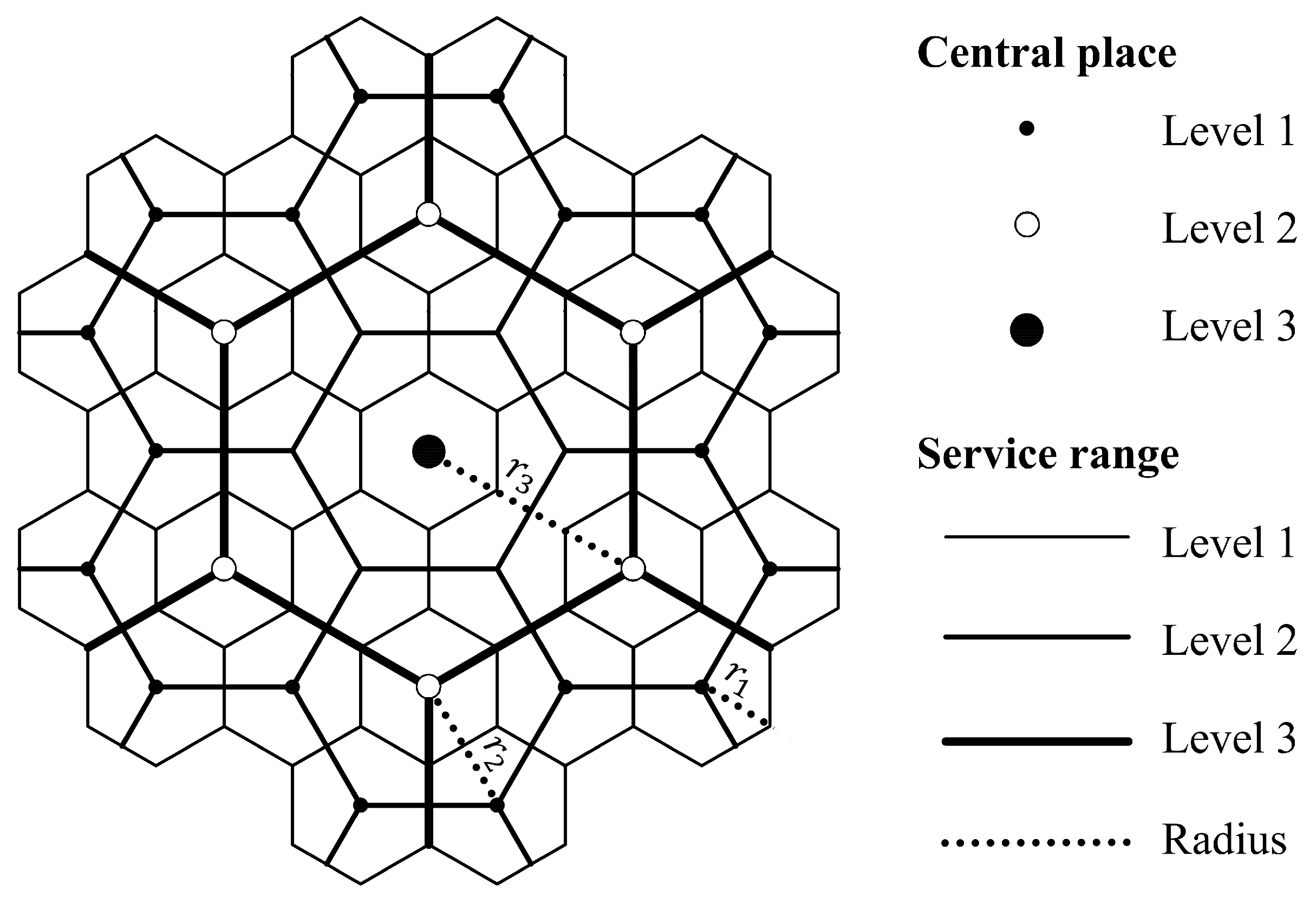
Figure 2.
Location of study area and distribution of sample points. (a) Location of China; (b) location of the study area in China; (c) distribution of sample points. NECP—northeastern China plain; NCP—north China plain; MLPYR—middle and lower reaches plain of the Yangtze River.
Figure 2.
Location of study area and distribution of sample points. (a) Location of China; (b) location of the study area in China; (c) distribution of sample points. NECP—northeastern China plain; NCP—north China plain; MLPYR—middle and lower reaches plain of the Yangtze River.

Figure 3.
Flow chart of the home-field straight-line distance (HFLD) calculation based on the Euclidean distance analysis tool.
Figure 3.
Flow chart of the home-field straight-line distance (HFLD) calculation based on the Euclidean distance analysis tool.

Figure 4.
Correlation analysis between the average home-field straight-line distance (HFLD), maximum HFLD, and latitude in the eastern plains of China (EPC).
Figure 4.
Correlation analysis between the average home-field straight-line distance (HFLD), maximum HFLD, and latitude in the eastern plains of China (EPC).

Figure 5.
Average and maximum home-field straight-line distances (HFLDs) in the eastern plains of China (EPC). NECP—northeastern China plain; NCP—north China plain; MLPYR—middle and lower reaches plain of the Yangtze River.
Figure 5.
Average and maximum home-field straight-line distances (HFLDs) in the eastern plains of China (EPC). NECP—northeastern China plain; NCP—north China plain; MLPYR—middle and lower reaches plain of the Yangtze River.
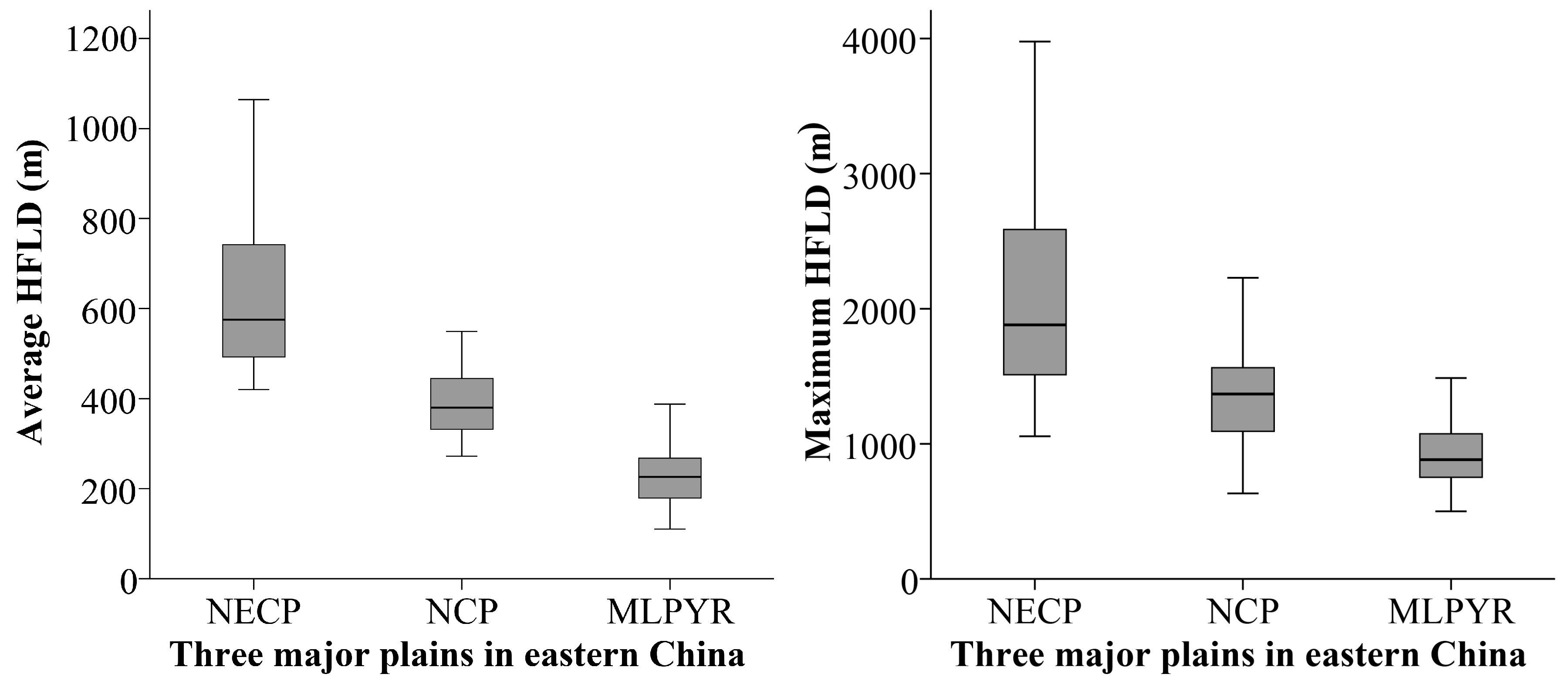
Figure 6.
Hot spot analysis results for the average and maximum home-field straight-line distances (HFLDs) in the eastern plains of China (Note: CF is confidence level).
Figure 6.
Hot spot analysis results for the average and maximum home-field straight-line distances (HFLDs) in the eastern plains of China (Note: CF is confidence level).

Figure 7.
Average patch number and area of rural settlements in the eastern plains of China (EPC). NECP—northeastern China plain; NCP—north China plain; MLPYR—middle and lower reaches plain of the Yangtze River.
Figure 7.
Average patch number and area of rural settlements in the eastern plains of China (EPC). NECP—northeastern China plain; NCP—north China plain; MLPYR—middle and lower reaches plain of the Yangtze River.
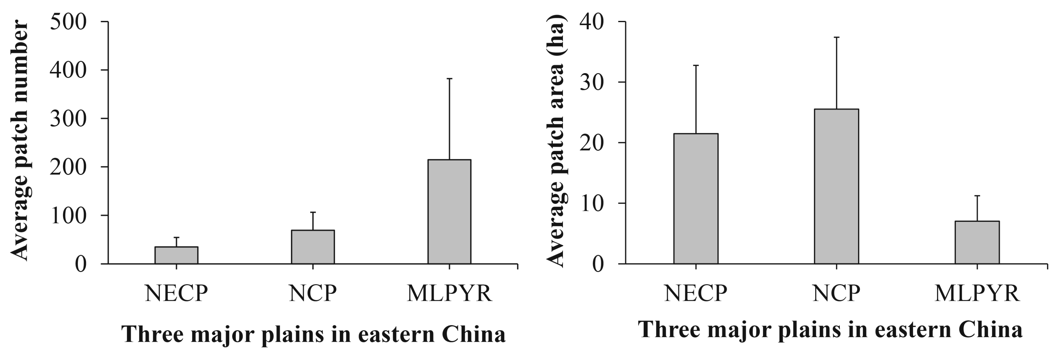
Figure 8.
Hot spot analysis results of the average patch number and area of rural settlements in the eastern plains of China (Note: RS is rural settlements; CF is confidence level).
Figure 8.
Hot spot analysis results of the average patch number and area of rural settlements in the eastern plains of China (Note: RS is rural settlements; CF is confidence level).

Figure 9.
Average nearest neighbor analysis results for rural settlements in the eastern plains of China (EPC).
Figure 9.
Average nearest neighbor analysis results for rural settlements in the eastern plains of China (EPC).

Figure 10.
Farmers’ travel modes and travel routes in the eastern plains of China (EPC) when a field is far away and goods need to be transported. HFPD—home-field path distance; HFLD—home-field straight-line distance.
Figure 10.
Farmers’ travel modes and travel routes in the eastern plains of China (EPC) when a field is far away and goods need to be transported. HFPD—home-field path distance; HFLD—home-field straight-line distance.


Table 1.
Percentage of farmland in different distances from the nearest rural settlement in the eastern plains of China (EPC).
Table 1.
Percentage of farmland in different distances from the nearest rural settlement in the eastern plains of China (EPC).
| Plains/Distance | 0–0.5 km | 0.5–1 km | 1–1.5 km | 1.5–2 km | >2 km |
|---|---|---|---|---|---|
| NECP | 45.8% | 34.5% | 12.6% | 4.5% | 2.7% |
| NCP | 74.3% | 22.3% | 3.0% | 0.3% | 0.1% |
| MLPYR | 92.1% | 7.5% | 0.4% | 0.0% | 0.0% |
Note: NECP—northeastern China plain; NCP—north China plain; MLPYR—middle and lower reaches plain of the Yangtze River.
© 2019 by the authors. Licensee MDPI, Basel, Switzerland. This article is an open access article distributed under the terms and conditions of the Creative Commons Attribution (CC BY) license (http://creativecommons.org/licenses/by/4.0/).
Share and Cite
MDPI and ACS Style
Li, X.; Liu, Y.; Chen, Y.; Li, P.; Yu, Z. Village Regrouping in the Eastern Plains of China: A Perspective on Home-Field Distance. Sustainability 2019, 11, 1630. https://doi.org/10.3390/su11061630
AMA Style
Li X, Liu Y, Chen Y, Li P, Yu Z. Village Regrouping in the Eastern Plains of China: A Perspective on Home-Field Distance. Sustainability. 2019; 11(6):1630. https://doi.org/10.3390/su11061630
Chicago/Turabian StyleLi, Xuedong, Yunhui Liu, Yajuan Chen, Pengyao Li, and Zhenrong Yu. 2019. "Village Regrouping in the Eastern Plains of China: A Perspective on Home-Field Distance" Sustainability 11, no. 6: 1630. https://doi.org/10.3390/su11061630
Note that from the first issue of 2016, this journal uses article numbers instead of page numbers. See further details here.