How to Effectively Enhance Sustainable Livelihoods in Smallholder Systems: A Comparative Study from Western Kenya


1
Systems Theme, World Agroforestry Centre (ICRAF), P.O. Box 30677, 00100 Nairobi, Kenya
2
Soils Theme, World Agroforestry Centre (ICRAF), P.O. Box 30677, 00100 Nairobi, Kenya
3
UNEP DTU Partnership, 2100 Copenhagen, Denmark
*
Author to whom correspondence should be addressed.
Sustainability 2019, 11(6), 1564; https://doi.org/10.3390/su11061564
Submission received: 23 January 2019
/
Revised: 1 March 2019
/
Accepted: 9 March 2019
/
Published: 14 March 2019
(This article belongs to the Special Issue Sustainable Development of Tropical Agriculture)
Abstract
:Increasing communities’ adaptive capacity is crucial to enhancing the sustainability of livelihoods and landscapes in smallholder systems. This study evaluates the contributions of an asset-based community-driven local development project, which has an objective to enhance farmer livelihoods through context-specific agricultural and agroforestry training, in line with farmers’ identities, interests, and preferences. The project was implemented in two areas of the wider Nyando river basin: the Lower and Middle Nyando sites. The project effects on farmer livelihoods were evaluated by analyzing overall income enhancement through the adoption of climate-smart agricultural practices via the computation of total values of harvest. Socioeconomic data from 183 households, half of which were involved in the project, were considered. The findings showed that locality played an important role in the adoption and success of good agricultural practices. Additional significant positive factors included project participation, size of land operated, horticulture farming, livestock ownership, ownership of a title deed, hours worked, and crop species richness. The number of years farmed had a significant negative correlation with the value of harvest. Considering the stark differences in livelihood effects in both sites, researchers conclude that external support for climate-smart agriculture uptake needs to be considerate of, and respond to, biophysical and socioeconomic context.
1. Introduction
The adaptive capacity of smallholder farmers can be improved by targeting outcomes that positively influence the ability of communities to overcome climate-related constraints and other barriers to development [1]. Much of the climate change adaptation literature indeed argues that general well-being enhancement is most effective in raising adaptive capacity [2,3,4]. Considering that the primary livelihood source of the majority of western Kenyans is smallholder farming [5], increased on-farm income through improved agricultural practices can directly contribute to increased well-being.
However, projects that promote yield-improving crop technologies have experienced mixed success for a host of reasons. For example, they failed to take into account that economic status, land rights, and land tenure affect farming methods and agricultural investment employed by households and hence also affect crop yields [6]. Second, considering most farmers rely on rain-fed agriculture, fluctuation in rainfall and delayed onset of rains can result in lower crop yields and potentially lead to food insufficiency when not taken into account in project design [7]. Third, risk and risk perceptions concerning environmental conditions such as unusual drought occurrence, as well as uncertain market prospects, can hamper adoption by farmers [8]. Fourth, uptake of certain practices, including agroforestry, can be affected by worries that the introduction of trees on farms might reduce productivity of other crops [1]. Fifth, socioeconomic conditions, political dynamics, and other structural factors influence a household’s access to assets. It follows then that asset availability influences the ability to invest in particular technologies and to engage in certain livelihood activities that in turn influence the capacity to adapt to adverse effects of climate change in the present and future [9]. Finally, recommended practices are often not suited for a particular agroecology and contribute to increased land degradation and affect long-term land productivity [10]. Consequently, even when there are short-term gains in productivity, the long-term sustainability of farming systems and livelihoods is likely to be compromised [11].
For these reasons, it is imperative that agricultural management programs are tailored to guarantee long-term sustainability, an endeavor that is even more pressing in view of the present and predicted changes in climate. Both the definition of suitable climate-smart practices that potentially increase on-farm income, as well as the likelihood of uptake of these practices, depend on context. As this study will show, sound analysis of context is essential for the definition and promotion of successful, efficient, and sustainable activities, and proposed options ought to be in line with, and responsive to, local realities [12].
Climate-smart agriculture (CSA) has been proposed as a potential solution that could achieve the twin objectives of improving productivity and food security. It also has the potential to meet climate goals and therefore improve the sustainability of communities and landscapes. CSA is defined as programs or field management practices that (i) sustainably improve agricultural productivity and food security; (ii) improve adaptive capacity and resilience of farming systems; and (iii) mitigate the emission of greenhouse gasses (GHG) or sequester carbon in landscapes [13,14]. To qualify as CSA, agricultural practices must be context-specific and responsive to the priorities of the communities where they are introduced [15]. Instead of proposing a generalized list of CSA practices, “climate-smartness”, as a set of agricultural and land management practices, must be established through a process in which various scientific and local knowledge sources interact and exchange. In the global South, there is growing recognition that the pursuit of mitigation objectives might interfere with CSA objectives of food security and well-being [11]. In this vein, Bell et al. [16] proposed to center CSA around sustainable food production and resilience planning with GHG mitigation considered as a co-benefit. To satisfy the former, a step-wise process in which suitability for a given agroecological and climatic context is established before turning to socio-economic constraints and farmer interests and preferences.
Asset-based community-driven development (ABCD) is an approach and a set of tools that puts context-specificity at the forefront of rural development and sustainability promotion. ABCD tools help communities define their own development priorities in line with their various assets based on, and responsive to, their identities (who they are), interests (their rational calculations), and their preferences (what they like) [17]. ABCD approaches to international development, drawing on earlier work focusing on the empowerment of hundreds of communities across the United States [18], were comprehensively adapted by the Coady International Institute [19,20,21,22]. ABCD is theoretically embedded in, and closely related to, the theory and practices associated with community economic development and endogenous development [23], participatory rural appraisal (PRA) and self-mobilizing techniques [3], the field of Appreciative Inquiry [24,25], ‘Positive Deviance’ [26], and the Sustainable Livelihoods Approach [27]. Philosophically, the approach is a critique of needs-based and problem-focused approaches that have dominated the development field. The approach deliberately considers and builds on context before any outside assistance is offered. External partners who promote community-driven development build awareness and facilitate the use of existing assets and opportunities, as opposed to defining problems and identifying gaps which supposedly require an outside organizations’ involvement [28].
The asset-based community-driven development project analyzed in this paper aimed to improve farmer resilience through the promotion of community-selected, context-specific CSA practices. In line with the context-specificity requirement of CSA, these practices were not pre-defined or pre-set but the result of a longer engagement process. First, priorities in terms of target sub-sectors were defined jointly with communities. Within these sub-sectors, various practices were promoted. The specific practices related to these sub-sectors resulted from a process that involved knowledge exchange and co-creation by bringing together ICRAF’s technical knowledge, the knowledge of government extension officers, and local knowledge and experience from ‘farmer trainers’ recruited from the locality because they had excelled in the practices in question and provided a voice to the project from farmers themselves.
Since ICRAF’s technical knowledge and priorities revolve around ‘natural farming’ technologies as much as possible, one field-level practice that was emphasized in the project was agroforestry. Agroforestry, defined as trees planted or intentionally managed on farms and ranches [29], was selected because of the multiple benefits it delivers to small-scale farmers. These include carbon sequestration, soil structure improvement, modification of the microclimate, and income generation [1,30,31,32]. For these reasons, agroforestry is a central CSA practice in Sub-Saharan Africa [10,15]. Horticulture farming was another core priority for project groups.
In the project, both landscape and livelihood sustainability were directly addressed by supporting engagement in context-relevant practices through self-driven techniques and technologies, which researchers premised would be more likely to be taken up and to be successful. The project furthermore used producer-led value-chain analysis tools to align asset-based and market-driven considerations. The project worked with four farmer groups, two in Lower and two in Middle Nyando, between 2010 and 2014. This study assessed the project’s contribution to reducing climate change vulnerability, improving livelihoods, and enhancing overall sustainability of communities and landscapes. Specifically, researchers analyzed the project effects on agricultural practice and performance expressed in on-farm crop productivity, value of harvest, and income generated through agricultural sales.
The study sought to answer three questions: (i) How did the promotion of context-specific and self-selected agricultural practices affect livelihoods among project participants? (ii) Which factors determined positive livelihood effects? (iii) In relation to the latter, in which contexts can ABCD approaches support the identification and engagement in practices that contribute to enhancing the sustainability of livelihoods and landscapes?
2. Materials and Methods
2.1. Research Sites
The study was conducted in two sites in the Nyando river basin, located in Kisumu and Kericho counties of western Kenya, where the project was implemented. The study sites lie within latitude 0°7′ N, longitude 34°24′ E, and latitude 0°24′ S, longitude 35°43′ E, respectively. Low crop yields, unreliable rainfall, and severe soil erosion characterize the Lower Nyando site, where elevation is at 1200 m above sea level and the average annual rainfall is 1000 mm [33]. The Middle Nyando site, located at approximately 1600 m above sea level and with an average annual rainfall of 1500 mm, has higher crop yields, cooler temperatures, and more evenly distributed rainfall [33]. The mean minimum and maximum annual temperatures range between 14 °C and 30 °C in the Lower Nyando site and between 11 °C and 29 °C in the Middle [34]. The rainfall pattern in western Kenya is bimodal, with peaks occurring during the long rains (April–May) and short rains (October–December) [35]. Farmers align planting seasons with the rains, with the main planting season occurring during the long rains, and the second planting season during the short. Harvesting typically takes place in July–August for crops planted during the long rains and in December–January for crops planted during the short rains. In addition to biophysical differences, ethnicities also vary across sites. Members of the Luo ethnic group are dominant in the Lower site, while members of both the Kalenjin and Luo ethnic groups inhabit the Middle site (see Table 1).
2.2. Data Collection
The study was conducted in 2013–2014 in Kericho and Kisumu counties. The selection of the study sites was in continuation with prior ICRAF work in the Nyando river basin. This study specifically was part of a larger, cross-sectional ‘research in development’ [12] project entitled “Making Carbon Finance Work for Rural Poverty Reduction” that operated from January 2010 to August 2014. After conducting preliminary focus-group discussions with all groups in November and December 2013, a household survey centering on respondents’ farm-related activities was carried out in January and February 2014. Data was collected on crop harvest and sales alongside various land management measures, namely; the use of chemical farm inputs, type of seed, irrigation frequency, soil fertility, and length of usage of land. The seasonal calendar in the area meant that the second harvest in 2013 was not complete and ready for sale by the time the survey was conducted, so the reference year 2012 was chosen.
To identify the project’s contributions to, or effects on, well-being through the promotion of CSA, data was collected in both sites in the Nyando river basin (Middle and Lower) where the project was implemented. In the Middle site, data was collected from members of two project groups. Two additional community groups in the same area were selected as Middle control groups. The identical process was followed in the Lower site. Project groups had initially been selected by the implementing team primarily based on their prior involvement in agroforestry. One project group in each region had been part of a prior ICRAF project, while the second project groups in each region had been selected based on demonstrated interest in agroforestry.
For each of the four project groups, one “suitable” control group was selected. While using “control” groups to assess treatment effects can be criticized for a myriad of reasons, it is recognized as a valid proceeding in social science research [36]. To establish suitability, community groups were sampled from the same neighborhoods, which were understood as being representative of ‘typical’ farmer groups in the area. A structured proceeding guided the selection of control groups. The most important suitability indicator was minimal contact with outside actors because it was assumed that the resulting collaboration, support, and activities would distort baseline quality.
A questionnaire comprising 15 categories was administered to all community groups that the local authority had mobilized for potential control group selection. These categories included the level of group income, average education of members, area of operation, physical assets of group members, average land acreage, mode of land preparation, food security, partnerships with outside organizations, and group accomplishments. The results were then weighted with regards to compatibility with the respective project group in terms of group size, ‘age’, gender distribution, social stratification, livelihood practices, and environmental conditions.
In the end, after an additional ground-truthing exercise, groups were selected in which location, dominant land use, average land size, and age of group members were similar to distributions in the respective project groups. In total, 183 respondents responded to the questionnaire from eight community groups, four in each site (Middle and Lower), of which two were from the project and two were control groups. After the ICRAF researcher conducted all preliminary research, including control group selection and various rounds of FGDs, a research team composed of 20 trained research assistants collected the survey data.
2.3. Data Analysis
In preparation for the analysis, outliers in the dataset were identified through visualization using a box plot. Later, outliers were confirmed through z-score tests. Observations with z-score values outside of the (−3, 3) range were considered outliers [37], and nine households were initially excluded. The values of outlying observations could have been smoothened, but the robustness check (results can be found in the Supplementary Materials) showed that the model would change considerably if the data were winsorized at 1% and missing values were replaced with the mean. Therefore, outliers were excluded from the main analysis (n = 174), herein referred to as the “clean” dataset. Due to the heterogeneous nature of small-scale farming systems, completely excluding outliers may, however, mask significant production value indicators. Hence, the full dataset inclusive of outliers (n = 183), herein referred to as the “raw” dataset, was analyzed as well (results from the “raw” dataset can be found in the Supplementary Materials).
Considering the importance of the biophysical context on land use and management, which rendered the Lower and Middle sites incomparable, project effects were compared throughout four sub-samples, namely, Lower Project (n = 45), Lower Control (n = 42), Middle Project (n = 48), and Middle Control (n = 39) for the “clean” dataset. In the “raw” dataset, the distribution across sub-samples was as follows: Lower Project (n = 46), Lower Control (n = 46), Middle Project (n = 50), and Middle Control (n = 41).
To evaluate the contributions of the project, a household’s income from agricultural production was used as the dependent variable. Agricultural income was defined as the total value of harvest; the sum of individual indications made about crop species planted and harvested on various plots, independently from whether these were sold or kept for other uses. The harvest volumes were further translated into monetary value by using standardized market prices for the target area. The total value of harvest for each household was computed using county average prices for Kisumu and Kericho Counties, which was obtained from the National Farmers Information Service [38]. While respondents provided the prices obtained from their sales, standardized county-specific prices were used for the year 2012 due to the high variance in self-reported prices. Simple descriptive statistics, including means and percentages, across the groups and sites were calculated. Analysis of variance (ANOVA) [39] was used to identify the differences between the control and project groups within the Middle and Lower sites using R Software version 3.4.0 [40].
Using the resulting data, two regression models were fitted with both the categorical and continuous variables to assess the project’s contribution on the response variable. These models also allowed researchers to identify the factors that influence farmer income and to account for potential differences and project effects across the two sites [41]. Based on the relevant literature [1,42,43,44], twelve indicators were selected as the main predictors of farmers’ income in the Nyando river basin: X1 (treatment, i.e., membership in project or control group), X2 (livestock ownership; specifically, the number of livestock owned was converted to tropical livestock units (TLU) per household member [45,46]), X3 (farm mechanization; specifically, if a tractor was used), X4 (average hours worked per week), X5 (gender of the household head), X6 (size of land operated), X7 (farming experience through number of years farmed), X8 (crop species richness), X9 (household size), X10 (importance of farming for household income; specifically. if farming was the main source of income), X11 (farming practices; specifically, if horticulture was practiced), and X12 (legal status of the land operated; specifically. ownership of a title deed for the land operated). Of these variables, six were categorical (X1, X3, X5, X10, X11, and X12) and six were continuous (X2, X4, X6, X7, X8, and X9).
Several multiple linear regression models were fitted to analyze the data by applying the following formula:
Y represents the farmers’ agricultural income, C is a constant, βi is the regression coefficients of the corresponding variable, Xi is the corresponding variable (with i ranging from 1 to 12), and ε is a random error term.
Due to non-normality of the data, natural logarithms were introduced to adjust for skewness in the continuous independent variables, and the response variable was winsorized to minimize the effect of outliers [47,48]. Stepwise regression was used to determine whether farmer income was influenced by the explanatory variables listed in the described model. Stepwise regression allowed researchers to avoid potential multi-collinearity among some of the explanatory variables, which would have violated the assumptions of multiple regression in the case that all twelve indicators were maintained [49]. Both forward and backward stepwise regression was applied to ascertain whether model selection procedures affected the results. In every forward step, the explanatory variable with the highest t-statistic was added. In each backward step, the explanatory variable with the lowest t-statistic was removed through step function of the statistics package in R [50].
3. Results
In line with general practice, only statistically significant results (p < 0.01; 0.05.; 0.1) are discussed in this section. In a few instances, results that are not statistically significant are mentioned and are clearly marked as such.
3.1. Household and Livelihood Characteristics
The average farm size owned was 1.13 ha across the entire sample: 1.21 ha and 1.05 ha in the Middle and Lower Nyando sites, respectively. The size of land operated was larger (p < 0.01) in the Middle site with 0.93 ha compared to 0.65 ha in the Lower. The average household size was seven, with 70% headed by men. Interestingly, women headed considerably more households in Lower Nyando (44%) than in Middle Nyando (17%). All Lower Nyando households belonged to the locally dominant ethnic group, Luo. The farmers in the Middle Nyando groups were either of the Luo and Kalenjin ethnic groups, with the Kalenjin being the majority.
Group members in Middle Nyando used a higher proportion of their land for crop and livestock farming (over 75% of land owned). The most common species of livestock reared were indigenous chickens (86% of the households), with cattle, sheep, and goats being the other commonly kept livestock. Livestock populations were converted into tropical livestock units (TLU) [45,46]. The overall mean TLU was 2.77, with higher values (p < 0.01) found in the Middle site.
Farmers derived livelihoods from a combination of sources. These included crop sales, subsistence agriculture, livestock production, small businesses, casual labor, and the sale of artisanal products. Comparison across sites showed that more farmers in the Middle site listed subsistence farming (p < 0.01) and engagement in casual labor (p < 0.05) as a source of income. Land was mainly tilled by hand (54%) or with an animal-powered plough (67%), while only 15% reported to have used a tractor for land preparation at some point. Most respondents reported using more than one farm preparation method on their farms. The mean number of hours respondents worked was greater in the Middle site (p < 0.1) than in the Lower site.
In the Lower site, only 28% of the sample reported that farming was their main source of income compared to 53% in the Middle. Of these, two-thirds were from the project groups. Respondents in the Lower site also reported a higher number of years worked on their farms (p < 0.05) compared to those in the Middle site. The number of farmers who reported using irrigation in 2012 was low, with only 13% of the households stating that they irrigated their land at some point. Of these, 65% were in Middle site households.
3.2. Presentation of Agronomic Data
3.2.1. Total Value of Harvest
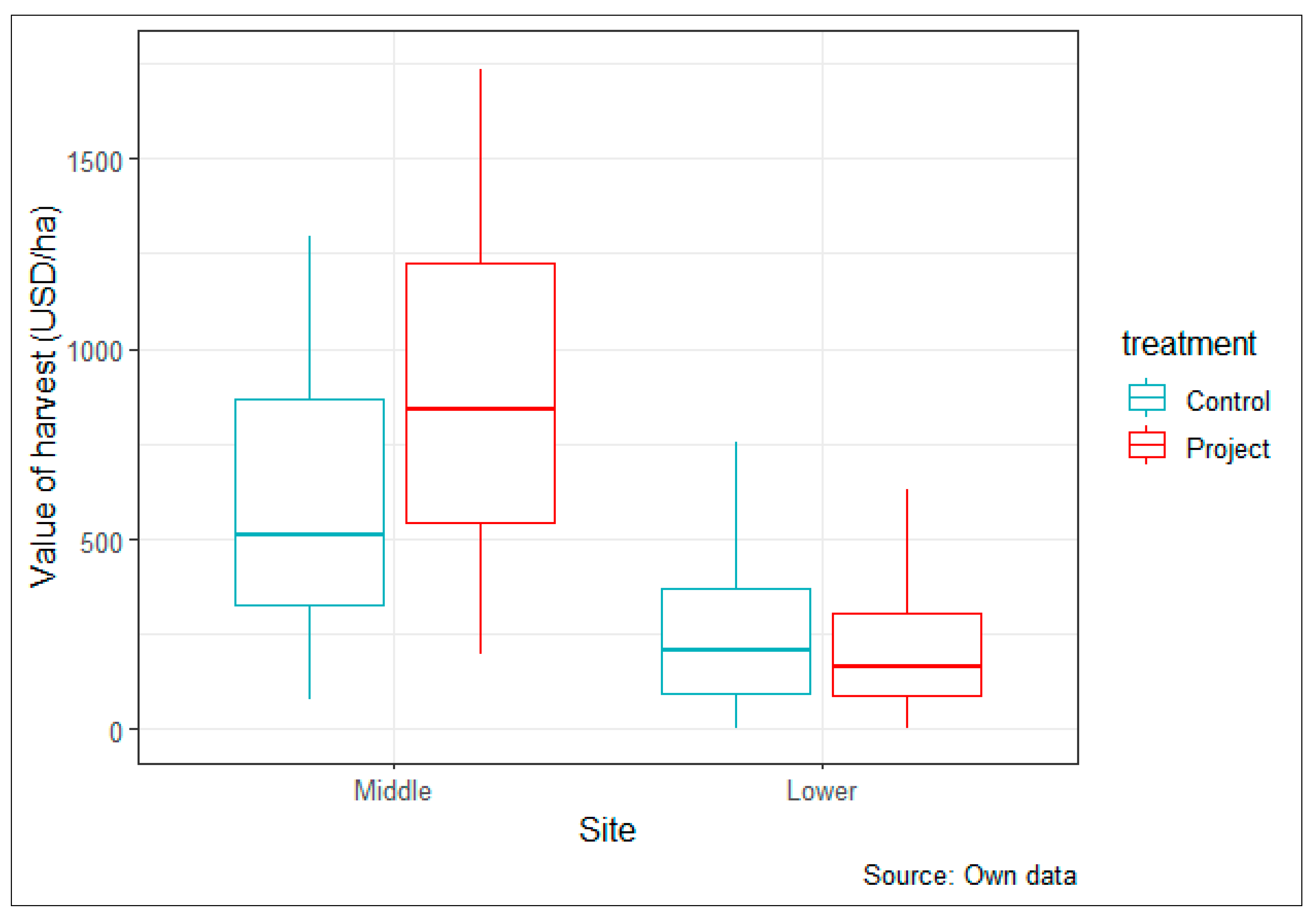
The mean value of harvest across the sites was 820 USD per hectare with reported mean sales of 320 USD for every hectare cultivated (see Table 1). This translates to an average value of 39% of the total harvest per hectare sold for income. Values of harvest were greatly influenced by a household’s location in either the Lower or Middle site. A one-way ANOVA analysis shows that the average value of harvest in Middle Nyando was considerably greater than in Lower Nyando (p < 0.01) (see Table 1 and Figure 1). Within the sites, the mean value of harvest of the Middle project group was greater than the Middle control group, although not statistically significant. Conversely, the mean value was greater in the Lower control group than the Lower project group (p < 0.1) (see Table 1).
The median total value of harvest represents the centrality of the values better because it reduces the influence of extremes. Accordingly, a series of Wilcoxon rank tests showed that the median value of harvest was greater in the Middle site (p < 0.1), while no significant difference existed in the Lower groups (Table 1 and Figure 1). Considering total self-reported income from crop sales, total sales in the Middle site were greater than in the Lower site (p < 0.01). While there were no significant differences in the total sales between the project and control group in the Lower site, the Middle project group had greater total sales (p < 0.05) than the control group (see Table 1). Project group households with the highest sale values reported cultivation of high value crops such as coffee, sugarcane, or tomatoes.
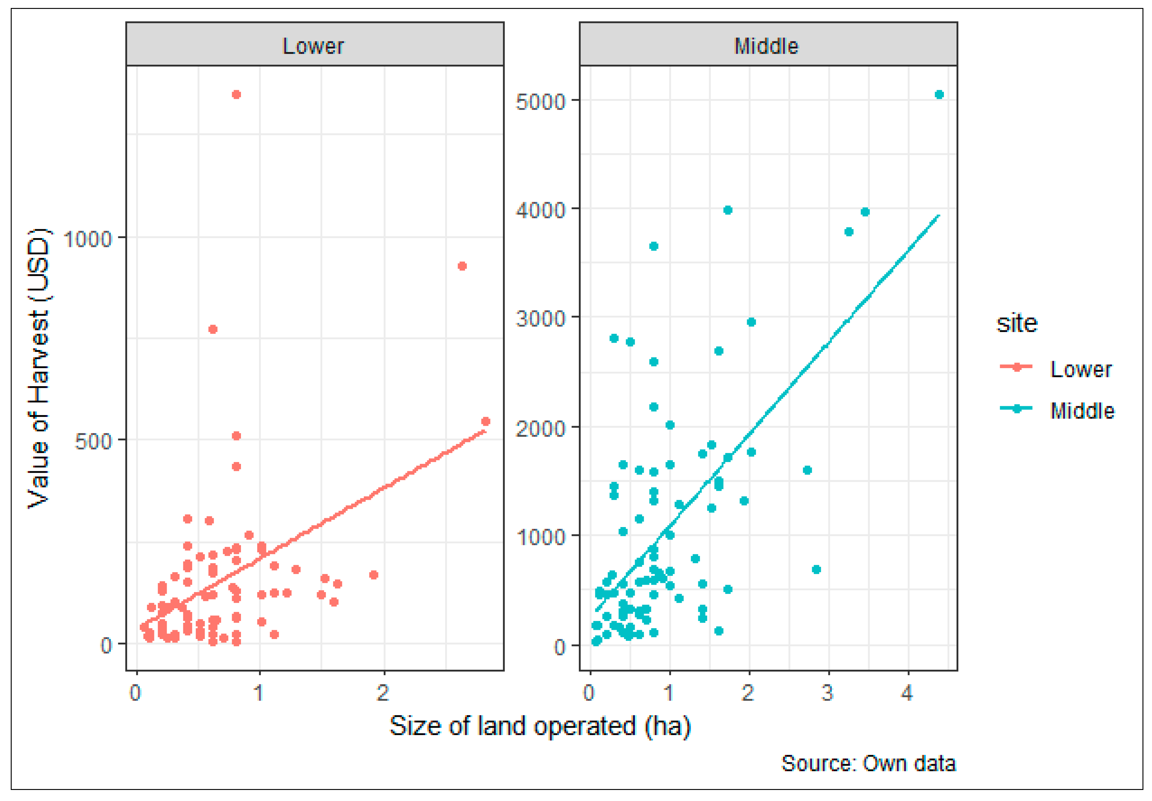
The value of harvest was also plotted against the land operated to identify if there was any linear relationship between the two variables (Figure 2) [51]. In the Lower site, there was a moderate positive relationship between land operated and the value of harvest (rho = 0.44, p < 0.01) and a strong positive relationship between land operated and the value of harvest (rho = 0.63, p < 0.01) in the Middle site. The graph below shows the relationship and the best-fit lines for both sites.
To compare yields across the various groups (see Table 1), maize was selected as the reference crop because it was the most commonly farmed across the sample. The average maize yield in the Middle site was greater than the yield in the Lower site (p < 0.01). The average maize yield in the Middle project group was greater than in the Middle control group, while the average yield in the Lower control was greater than in the Lower project group. However, differences between project and control groups in both sites were not statistically significant. The average maize yields were considerably lower than the expected actual yields published by the Global Yield Gap and Water Productivity Atlas [52] for the respective counties, with expected yields at 0.96 tons/ha in Kisumu and 2.60 tons/ha in Kericho.
3.2.2. Engagement in Horticulture Farming
The variable ‘contribution of horticulture’ was defined as the monetary value that horticulture contributed to the total harvest value of a household. The average value of contribution of horticulture to the total value of harvest across the sites was 182 USD per hectare operated. The average contribution of horticulture was 354 USD in the Middle site and differed from the contribution of 11 USD in the Lower site (p < 0.01) (see Table 1). Horticulture contributed to 26% of the total mean value of harvest in the Middle site (expressed as a proportion of the total mean value of harvest). In both sites, the difference in the contribution of horticulture between the project and control groups was insignificant. However, as discussed in the previous section, the mean value of harvest in Lower Nyando differed from Middle Nyando (p < 0.01). Considering the difference in horticulture engagement within the regions, the value of the horticulture harvest was omitted from each household and the resulting value of harvest per hectare was compared. First, the difference between the average value of harvest in the Lower region and Middle region remained highly significant (p < 0.01) (see Table 1). However, although the initial significance of differences between the Lower control group and the project group’s value of harvest was already considerable at p < 0.1, it rose to p < 0.05. Omitting the value of horticulture in the total value of harvest in Middle Nyando also resulted in a significant difference between Middle project and Middle control (p < 0.1) that did not exist in the mean total value of harvest (see Table 1). Comparing horticulture farming across sites, the number of households that indicated that they practiced horticulture was greater (p < 0.01) in the Middle region than in the Lower region. Furthermore, more farmers practiced horticulture in the Lower project group than in the Lower control group (p < 0.05) (see Table 1). The differences among the farmers who practiced horticulture and the size of land operated were also analyzed. In the Lower site, the mean size of land operated by horticulture farmers was 0.82 ha and 1.26 ha in the Middle site, which was a result of having bigger parcels of land (see Table 1).
3.2.3. Food Self-Sufficiency and Production Depression
Food self-sufficiency was explored and expressed as the number of months a household was able to sustain itself primarily on produce from its own farm [53]. The average number of months that households sustained themselves primarily on their own produce was 6.32 in 2012 and 4.73 in 2013 across the samples (Table 1). When comparing food self-sufficiency in the sites, the average number of months the households fed on their own produce was greater (p < 0.01) in the Middle than in the Lower site in both 2012 and 2013. In both sites, households from project groups fed on their own produce for longer than those from the control groups. This difference was particularly significant (p < 0.01) in the Middle site in both 2012 and 2013. A Pearson product-moment correlation coefficient was computed to assess the relationship between the number of months of food-sufficiency in 2012 and 2013. There was a strong, positive correlation (rho = 0.63, p < 0.01) between the average food self-sufficiency across the sites during these two years. Shorter food self-sufficiency in 2012 was correlated with shorter food self-sufficiency in 2013. Production depression was hence less pronounced among project households than among control households, particularly in the Middle site.
3.2.4. Food Plant Species Richness
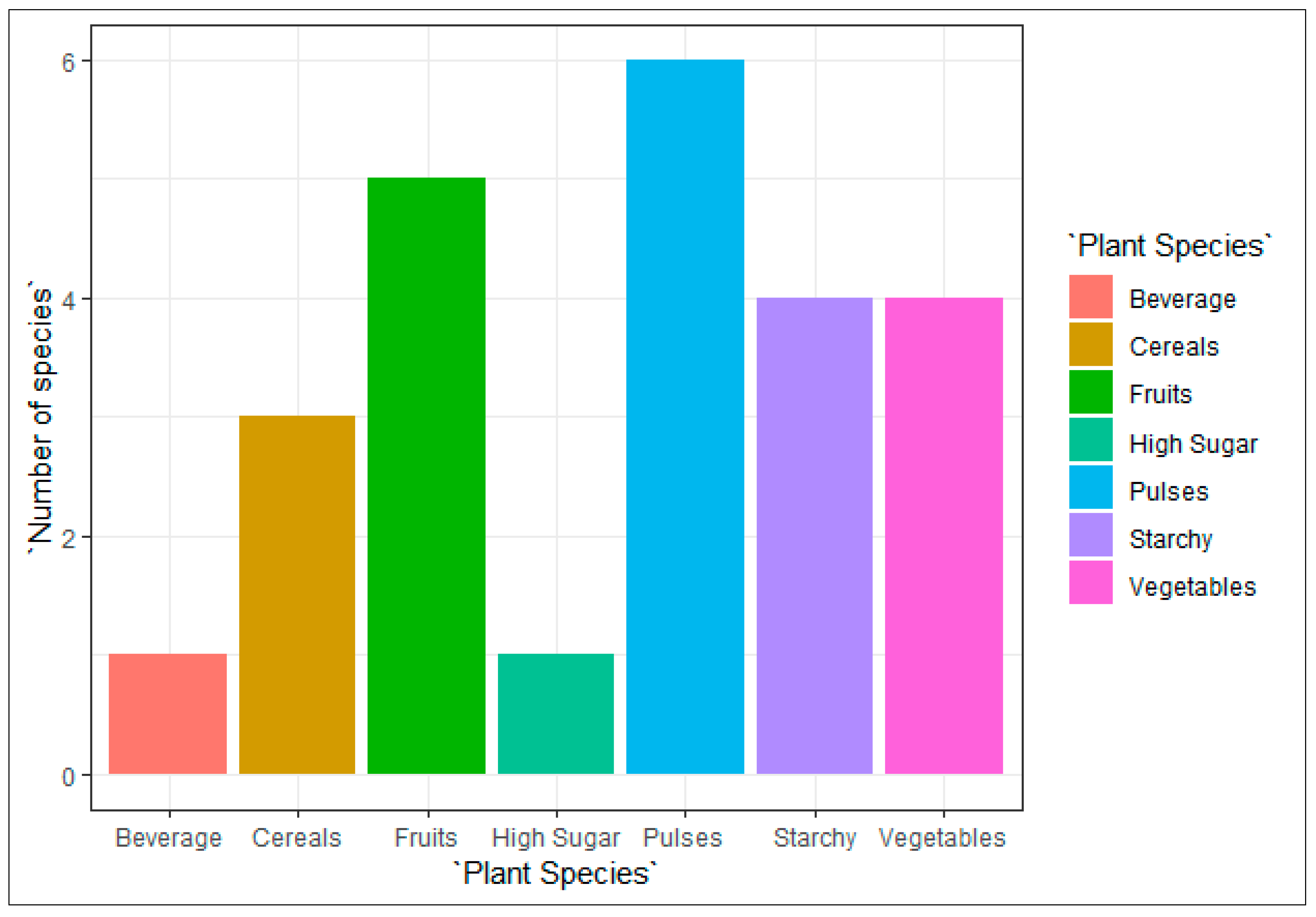
Across both the Lower and Middle Nyando sites, households planted 24 food plant species in 2012. All of the on-farm food plant species recorded were categorized according to the seven major Food and Agriculture Organization (FAO)-defined food plant groups, which are differentiated based on their nutrient content: (a) cereals, (b) vegetables, (c) starchy roots/tubers/green bananas, (d) pulses/nuts/seeds, (e) fruits, (f) spices/condiments/beverages, and g) high-sugar foods [54]. In the overall sample, the most common food plant groups were pulses (e.g. beans, green grams, cow peas) and the least common were beverages (coffee) and high-sugar foods (sugarcane) (Figure 3). The most common intercrop combination in the Lower site was maize and sorghum, while maize and beans were most commonly intercropped in the Middle site, which is consistent with results from another study from the site [55].
Overall, the most commonly planted crop by individual households was maize (91%), with 98% of households in the Middle site and 85% of the households in the Lower site indicating to have planted the crop (Table 2). In line with the differences in agroclimatology in the two sites, the other most commonly planted and harvested crops differed between Lower and Middle Nyando (Table 2).
A series of chi-square tests of independence were performed to examine the relation between the food crop planted and the site (Lower or Middle). The relation between these variables was highly significant—X2 (1, N = 174), p < 0.01—for sorghum, beans, green grams, coffee, tomato, sugarcane, cowpeas, and groundnuts (Table 2). Considerably fewer farmers in the Middle site planted sorghum, green grams, cowpeas, and groundnuts; rather, they preferred planting beans, coffee, tomatoes, and sugarcane. The relation between planting maize and the site was significant—X2 (1, N = 174), p < 0.05—with markedly higher numbers of farmers in the Middle site farming maize. Within the sites, there were no significant differences apart from higher engagement in sorghum farming among Middle control farmers than among Middle project farmers.
The overall mean total of food plant species richness, which defines the average number of food crops species planted per household, was (3.13), with the mean of the Lower project group (2.71), differing from the mean total food plant species richness of the Lower control group (p < 0.05; 3.21) (Table 1).
3.2.5. On-Farm New Tree Plant Species Richness
To understand the nature of engagement in agroforestry, various aspects were considered. Altogether, almost all households across all sub-samples indicated having indigenous trees on their farms. Furthermore, 92% of all households indicated having planted trees during the five years prior to the study. The variable ‘on farm new tree plant species richness’ was defined based on self-reported data concerning tree species planted on the farm during the five years prior to the study. Project groups in both sites had planted more tree species than their control groups (p < 0.01) (Table 1) during this period.
3.3. Factors Influencing Value of Harvest
Initially, when using one model for both sites, the variable ‘site’ was a highly significant determinant of agricultural income. Since using one model would conceal important differences that result from varying climatic and biophysical characteristics between the two sites, separate models were fitted for each (Lower and Middle) to identify the strongest predictors of agricultural income, defined as total value of harvest per land size (ha).
For purposes of comparison, both the “raw” (183 observations) and “clean” (174 observations) datasets were analyzed. For the “raw” dataset, the stepwise regressions yielded four significant variables in the Middle site and five in the Lower site (results in Supplementary Materials). For the Middle site, the size of land operated (p < 0.01), number of years farmed (p < 0.1), treatment and involvement in the project (p < 0.01), and engagement in horticulture (p < 0.01) were significant. For the Lower site, size of land operated (p < 0.05), ownership a title deed (p < 0.1), crop species richness (p < 0.01), average hours spent on the farm per week (p < 0.05), and TLU per household member (p < 0.05) were significant.
For the “clean” dataset, the stepwise regressions yielded a higher number of significant variables per model. Cleaning the data hence improved the models. For the Middle site, the strongest predictors were treatment (involvement in the project), size of land operated, engagement in horticulture farming, number of years farmed, and TLU per household member. For the Lower site, TLU per household, size of land operated, ownership of a title deed, number of years farmed, crop species richness, and average hours spent on the farm per week were significant. Apart from farming experience, all factors influenced the production value positively (Table 3).
Altogether, of the 12 variables fitted in the full model, eight were significant predictors of total value of harvest in at least one of the sites in the final models. Only three factors—land size operated, farming experience, and TLU per member—had a significant effect in both locations. While the effect of land size operated and farming experience was comparable in both sites, TLU per household member influenced the value of harvest considerably more in the Lower than in the Middle site. Project involvement and engagement in horticulture farming were only significant in the Middle site. Ownership of a title deed, crop species richness, and average hours worked were only significant in the Lower site. None of the other variables fitted in the full model significantly influenced the value of harvest.
4. Discussion
When farmers allocate resources to their farm, they are likely to invest in activities that will bring the highest returns to cater for their family’s needs and priorities [56]. In view of the highly significant difference between total income per ha in Middle and Lower Nyando, as well as in specific farming practices, the climatic and agroecological differences between the sites are a primary criterion of concern for the engagement in, and promotion of, specific climate-smart activities [1].
Concerning these practices, in line with previous studies [1], the results from the Middle site illustrate the considerable benefit drawn from engagement in horticulture farming, including fruit tree planting. Indeed, it contributed one quarter of the total value of harvest in the Middle site, as reported in Section 3. The promotion of horticulture is hence sensible if farmers can meet the requirements for reliable production. In the Middle site, it is thus likely that horticulture’s high profitability boosted increased repeat investments, which is a strategy capable of improving livelihoods with new project groups going forward. Considering the importance of risk-averseness related to uncertain environmental conditions, it is important to promote these practices in a context of sustainable intensification in line with farmers’ assets and interests, since it is essential that farmers learn how to intensify production without degrading the soil. This can help address the problem of reducing available farmlands by enhancing sustainable intensification, better optimizing production of smallholder farms, and therefore potentially increasing the value of harvest and income [57,58]. Apart from engaging in climate-smart practices related to cereal and horticulture crop farming, adoption of agroforestry can be an important tool to improve soils while also improving farm yields and mitigating the adverse effects of climate change.
High adoption rates and greater new on-farm tree species diversity in the Middle site also confirm that agroforestry promotion is most successful when introduced simultaneously with practices that allow for faster returns and short-term benefits. Again, horticulture cultivation is one practice that resulted in higher sales for farmers in this project [59]. By providing livelihood benefits from faster-growing crops, the gap to the future benefits of the trees, including shade, fruits, and wood fuel can be bridged, and farmers’ interest in agroforestry can be increased.
Beyond locality, the study found several determinants that influenced the value of harvests either positively or negatively. The strongest positive predictor of the value of harvest in both sites was the size of the land operated. This result reinforces other studies that, for instance, show that higher returns of those operating larger farms depend on better access to capital and non-labor variable inputs [60]. The results might also indicate that more intensive farming cycles on smaller farms can lower land productivity and lead to a lower value of harvest per ha. Research has shown that farmlands in western Kenya, as elsewhere in the country, are under substantial pressure due to steeply rising population numbers [61]. This socio-spatial transformation renders sustainable land use and management technologies and practices all the more important.
The second factor was TLU per household member, which was significant in both sites. This variable is used as one of the proxies for wealth in agricultural societies [45]. Households with a higher value are considered wealthy. This result proves the relationship between income and TLU, confirming the suitability of using TLU per household member as a proxy for farm income and household wealth. The positive role of livestock in the value of harvest is furthermore in line with studies that treat livestock as a proxy for financial capital. Small livestock can easily be liquidated to smoothen consumption [62], while bigger livestock, particularly cattle, act both as a savings account and opportunity for larger investments [63]. The fact that the effect of TLU on income was considerably stronger in the Lower site might indicate that TLU is a more suitable proxy for income and wealth in drier areas than in more humid ones.
A further predictor of the value of harvest was farmer involvement in the project, although only in the Middle site. While different explanatory patterns might be invoked, it is plausible that the project groups in Lower Nyando engaged less in on-farm activities than the control groups because environmental and agroecological conditions in the area were not conducive for farming. Members of project groups in the Lower site might have decided to engage in activities that are more suitable for the area (and hence more context-specific), and diversify out of farming, leading to reduced harvest values.
A second factor in the Middle site was engagement in horticulture farming, a highly profitable undertaking when operationalized correctly. The high average total value of harvest and sales in the Middle control group (see Table 1) illustrate this point succinctly. Engagement in horticulture raised the Middle control group members’ income and lifted their value of harvest to levels that are comparable with Middle project members’. Horticultural production and consumption, alongside the income generated from these activities, contributed to closing nutritional gaps of these households, which is in line with previous studies [64].
Lastly, another major advantage of growing fruit trees, a part of horticultural production in our study, is the positive role it plays in climate change mitigation, which is also in line with previous studies [31]. Due to the sensitivity of some horticultural plants and the need for reliable irrigation and farm input supply, engagement in horticulture farming is only sensible when the production requirements are met. In this light, horticulture farming might not have positively affected income in the Lower site because sustainable production criteria were not given.
In the Lower site, three additional factors had effects on farm income at a 5% significance level. The first was ownership of a title deed, which is consistent with previous studies that show that tenure rights, backed by title deeds, motivate farmers to invest in their farms over the long term [65,66]. Furthermore, ownership of a title deed allowed farmers to access credit facilities by using their deeds as collateral. It is therefore likely that farmers who had a title deed in the Lower Nyando site invested more on their farms and hence earned higher returns. Since possession of a title deed did not have any significant effect on income in the Middle site, where overall crop production was much higher, the importance of having formal ownership rights to the land operated seems to be contextual and not universally applicable as often postulated [65,67,68].
The second factor in the Lower site was food crop species richness. This result is in line with a much more complex study from Malawi, which proves that greater on-farm agricultural biodiversity is correlated with greater household diet diversity, which can nutritionally support household members that provide necessary labor [69]. This study also suggests that promoting on-farm crop diversity provides farmers with additional opportunities to engage with markets, as they have more to offer and potentially contribute to increased income [69]. Crop diversification is also recognized as a measure that allows households to mitigate their vulnerability to external shocks, such as climate change [70]. The number of food crop species planted on-farm had a moderate that farmers with bigger plots of land planted a wider variety of food crops than those with smaller plots. This finding is confirmed by other studies [71].
The third factor was the average hours that farmers indicated having worked on their farm per week. In a context of little mechanization of farming practices, this correlation was to be expected. Despite this positive relation between labor and income, studies have shown that in most developing countries, Kenya included, work performed by men, women, and children on the farm is often unpaid [72] and therefore not represented as a production cost. Future studies could show how income computations change when all costs, including unpaid labor, are factored into the calculation of farm profit. The slightly higher degree of mechanization in the Middle site might have contributed to a lower importance placed on hours worked.
Regarding negative correlations between variables fitted in the model, the number of years farmed had a negative effect on the value of harvest in both sites. These results are interesting because they counter the common assumption that more experience leads to higher farm income. A possible explanation for this negative correlation is that the soils in land that has been farmed for longer periods are depleted of nutrients. In a context where land sizes are small and land is seldom left fallow and often insufficiently managed for replenishment, this depletion of nutrients may lead to lower productivity [73]. The negative correlation is also in line with other studies that show that older farmers with more farming experience are often more risk-averse and hence hesitant to adopt new farming techniques [74].This finding might have contributed to lower harvest volumes, particularly in a context of climate change. These results are also in line with the assumption that younger farmers are more willing to adopt innovative, climate-smart practices, which can translate into higher harvest values [75,76].
The study clearly shows that ABCD contributed to project group members’ engagement in agricultural activities that led to positive livelihood outcomes in Middle Nyando. The results obtained from data collected among the Lower Nyando project groups provide another interesting perspective on the ABCD approaches’ potential to support sustainable livelihood enhancement in smallholder systems, particularly in the context of climate change and uncertainty. Farmers in the Lower Nyando reported that rainfall in 2012 was less reliable than previously and that climatic unpredictability had increased in recent years [33], which is in line with expected climate change effects in the wider Nyando river basin [55]. In line with these findings, our data consistently shows lower engagement in farming among project group members in the Lower site compared to the control group members, and lower values of harvest. While at first, this finding might seem as if the project failed in these areas, it might indeed be more likely that both were the result of households’ conscious decision to diversify out of farming, since returns on investment were highly uncertain. As part of the ABCD process, project groups in Lower Nyando prioritized off-farm activities, namely, small-scale business, such as the sales of shoes, purchased vegetables, and second-hand clothes, over engagement in farming. In this vein, our data shows that only a quarter (24%) of the Lower project group sample reported farming as their main source of income compared to a third (31%) of the Lower control group sample. Beyond increasing the likelihood of reaping direct benefits from these off-farm engagements, off-farm income also allows farmers to acquire initial capital to fund on-farm activities, particularly those that require higher up-front expenses, such as engagement in horticulture, or activities where financial benefits are not as immediate, such as agroforestry [77,78]. While the direct increase in well-being through engagement in the project might not have translated in terms of increased value of harvest, increased understanding of available assets and opportunities might indeed have contributed to further diversification and increased resilience among Lower project group members.
5. Conclusions
Various methods were used to analyze the ways in which sustainable livelihoods can be promoted in smallholder systems. These methods allowed researchers to uncover the effects of contextual biophysical and socioeconomic factors on livelihoods. The study showed that smallholder farmers’ value of harvest was directly linked with their livelihoods and hence with adaptive capacity. Specifically, the study looked at whether asset-based approaches to encouraging engagement in context-specific activities, particularly engagement in CSA practices, affected smallholder farmers’ resilience to climate change.
The results show that the ABCD approach is useful in identifying and delivering CSA options that sustainably improve smallholder farmers’ livelihoods. CSA targets improved productivity and enhanced adaptive capacity and GHG mitigation. The ABCD project enhanced two of these three target outcomes: increased income among project group members, alongside a significant improvement in the ability of farming systems to withstand climate risks. This is, for instance, visible in project farmers having lower production depression compared to the non-project farmers during seasons with reduced rainfall. This is most likely related to project farmers having diversified farming systems, which spreads risks, a key indicator of improved adaptive capacity. As shown, the positive effect of the promotion of CSA on the sustainability of livelihoods and landscapes was particularly salient in the Middle site.
Considering the factors that determined success in agricultural engagement, a total of eight factors were identified across the sites that had been separated according to locality due to the importance of agroecological difference across the Nyando basin. Three of these were cross-cutting; the size of the land under operation and TLU per household member had a positive; and a farmer’s age had a negative effect on the total value of harvest. Beyond that, project involvement and horticulture farming were highly significant in the Middle, and ownership of a title deed, crop species richness, and labor input were significant in the Lower site.
Concluding on the suitability of ABCD to promote sustainability, the study results show that the implementation of ABCD approaches can indeed allow external actors to support diverse and diversified, context-specific, and sustainable livelihoods and landscapes. In line with Fuchs et al. [17], the study shows that external partners, however, must ensure that the skills, knowledge, and innovation they have to offer is relevant to the farmers they seek to support. Matching one’s offer with the communities’ identities, interests, and preferences (IIP) is critical. On the contrary, external actors whose ‘profile’ and ‘offer’ are not in line with the communities’ IIP might even hinder community development by setting artificial priorities and by contributing to means, concentration, and energy being diverted away from more worthy engagements. When targeted correctly, ABCD approaches can support the selection of CSA practices that promote sustainable intensification and potentially lead to increased productivity, which is key in an overall context of exponentially reducing farm sizes. Further studies can provide insights into the ABCD approach’s contribution to quantifiable benefits of GHG mitigation and carbon sequestration. ABCD can hence make an important contribution to providing options to current problems faced in agriculture and food security in the global South.
Supplementary Materials
The following are available online at https://www.mdpi.com/2071-1050/11/6/1564/s1.
Author Contributions
Conceptualization, L.E.F. and H.N.; data curation, L.O. and N.N.; formal analysis, L.O. and N.N.; funding acquisition, L.E.F. and H.N.; investigation, L.E.F.; methodology, L.E.F., L.O., N.N., and H.N.; project administration, L.E.F.; resources, L.E.F.; software, L.O. and N.N.; supervision, H.N.; validation, L.E.F., L.O., N.N., and H.N.; visualization, L.O.; writing—original draft, L.E.F. and L.O.; writing—review and editing, L.E.F., L.O., and H.N.
Funding
This work was supported by the Comart Foundation, a private Canadian charitable foundation, through the Coady International Institute.
Acknowledgments
The authors thank Tesfamicheal Wossen (IITA), Brian Chiputwa (ICRAF), ICRAF field staff Victoria Apondi and Langat Kipkorir, other colleagues who contributed to data collection, and Brianne Peters (Coady Institute) for proof reading this paper.
Conflicts of Interest
The authors declare no conflict of interest.
Disclosure Statement
The authors declare that they do not have any financial interest or benefit arising from the direct applications of their research.
References
- Thorlakson, T.; Neufeldt, H. Reducing subsistence farmers’ vulnerability to climate change: Evaluating the potential contributions of agroforestry in western Kenya. Agric. Food Secur. 2012, 1, 15. [Google Scholar] [CrossRef]
- Adger, W.N. Vulnerability. Glob. Environ. Chang. 2006, 16, 268–281. [Google Scholar] [CrossRef]
- Chambers, R.; Conway, G. Sustainable rural livelihoods: Practical concepts for the 21st century. IDS Discuss. Pap. 1991, 296, 1–29. [Google Scholar]
- Conway, G.; College, I. The science of climate change in Africa: Impacts and adaptation. October 2009, 1–24. [Google Scholar]
- Boye, A.; Verchot, L.; Zomer, R. Baseline Report Yala and Nzoia River Basins: Western Kenya Integrated Ecosystem Management Project Findings from the baseline SURVEYS; World Agroforestry Centre: Nairobi, Kenya, 2008. [Google Scholar]
- Place, F. Land Tenure and Agricultural Productivity in Africa: A Comparative Analysis of the Economics Literature and Recent Policy Strategies and Reforms. World Dev. 2009, 37, 1326–1336. [Google Scholar] [CrossRef]
- Mugalavai, E.M.; Kipkorir, E.C.; Raes, D.; Rao, M.S. Analysis of rainfall onset, cessation and length of growing season for western Kenya. Agric. For. Meteorol. 2008, 148, 1123–1135. [Google Scholar] [CrossRef]
- Current, D.; Lutz, E.; Scherr, S.J. The costs and benefits of agroforestry to farmers. World Bank Res. Obs. 1995, 10, 151–180. [Google Scholar] [CrossRef]
- Jensen, J. Understanding the Links between Water, Livelihoods and Poverty in the Nyando River Basin, Kenya. Ph.D. Thesis, University of Florida, Gainesville, FL, USA, 2009. [Google Scholar]
- Lamanna, C.; Namoi, N.; Kimaro, A.A.; Mpanda, M.; Egeru, A.; Okia, C.; Ramirez-Villegas, J.; Mwongera, C.; Ampaire, E.; Asten, P.J.; et al. Evidence-Based Opportunities for Out-Scaling Climate-Smart Agriculture in East Africa; CCAFS Working Paper No. 172; CCAFS: Wageningen, The Netherlands, 2016. [Google Scholar]
- Lipper, L.; McCarthy, N.; Zilberman, D.; Asfaw, S.; Branca, G. (Eds.) Climate Smart Agriculture; Natural Resource Management and Policy; Springer International Publishing: Cham, Switzerland, 2018; Volume 52, ISBN 978-3-319-61193-8. [Google Scholar]
- Coe, R.; Sinclair, F.; Barrios, E. Scaling up agroforestry requires research “in” rather than “for” development. Curr. Opin. Environ. Sustain. 2014, 6, 73–77. [Google Scholar] [CrossRef]
- Neufeldt, H.; Jahn, M.; Campbell, B.M.; Beddington, J.R.; DeClerck, F.; De Pinto, A.; Gulledge, J.; Hellin, J.; Herrero, M.; Jarvis, A.; et al. Beyond climate-smart agriculture: Toward safe operating spaces for global food systems. Agric. Food Secur. 2013, 2. [Google Scholar] [CrossRef]
- Lipper, L.; Thornton, P.; Campbell, B.M.; Baedeker, T.; Braimoh, A.; Bwalya, M.; Caron, P.; Cattaneo, A.; Garrity, D.; Henry, K.; et al. Climate-smart agriculture for food security. Nat. Clim. Chang. 2014, 4, 1068–1072. [Google Scholar] [CrossRef]
- Rosenstock, T.; Lamanna, C.; Chesterman, S.; Bell, P.; Arslan, A.; Richards, M.; Rioux, J.O.; Akinleye, A.; Champalle, C.; Cheng, Z.; et al. The Scientific Basis of Climate-Smart Agriculture: A Systematic Review Protocol. 2016. Available online: https://cgspace.cgiar.org/handle/10568/70967 (accessed on 9 January 2019).
- Bell, P.; Namoi, N.; Lamanna, C.; Corner-Dolloff, C.; Girvetz, E.; Thierfelder, C.; Rosenstock, T.S. A Practical Guide to Climate-Smart Agricultural Technologies in Africa; CCAFS Working Paper No. 224; CCAFS: Wageningen, The Netherlands, 2018. [Google Scholar]
- Fuchs, L.E.; Peters, B.; Neufeldt, H. Identities, interests, and preferences matter: Fostering sustainable community development by building assets and agency in western Kenya. Sustain. Dev. 2019, 1–9. [Google Scholar] [CrossRef]
- Kretzmann, J.P.; McKnight, J.L. Building Communities from the Inside out: A Path Toward Finding and Mobilizing a Community’s Assets; The Asset-Based Community Development Institute: Evanston, IL, USA, 1993; ISBN 9780879461089. [Google Scholar]
- Mathie, A.; Cunningham, G. Who is driving development? Reflections on the transformative potential of asset-based community development. Can. J. Dev. Stu./Revue Canadienne Études Développement 2005, 26, 175–186. [Google Scholar] [CrossRef]
- Mathie, A.; Cunningham, G.; Puntenney, D. From Clients to Citizens: Deepening the Practice of Asset-Based and Citizen-Led Development; Mathie, A., Puntenney, D., Eds.; Coady International Institute: Antigonish, NS, Canada, 2009; ISBN 9780968072592. [Google Scholar]
- Ghore, Y. Producer-Led Value Chain Analysis: The Missing Link in Value Chain Development: A Tool for Effective Engagement of Small Producers; Coady International Institute: Antigonish, NS, Canada, 2015. [Google Scholar]
- Mathie, A.; Cunningham, G.; Peters, B. Asset-Based and Citizen-Led Development: Participant Manual; Coady International Institute: Antigonish, NS, Canada, 2017. [Google Scholar]
- Diochon, M.C. Entrepreneurship and Community Economic Development: Exploring the Link; Durham University: Durham, UK, 1997. [Google Scholar]
- Elliott, C. Locating the Energy for Change: An Introduction to Appreciative Inquiry; International Institute for Sustainable Development: Winnipeg, MB, Canada, 1999; ISBN 1895536154. [Google Scholar]
- Ashford, G.; Patkar, S. Beyond Problems Analysis: Using Appreciative Inquiry to Design and Deliver Environmental, Gender Equity and Private Sector Development Projects. Final Progress Report; International Institute for Sustainable Development: Winnipeg, MB, Canada, 2001; p. 22. [Google Scholar]
- Tufts University. Basic Field Guide to the Positive Deviance Approach. Available online: https://texashumanities.org/sites/texashumanities/files/Basic%20Field%20Guide%20to%20the%20Positive%20Deviance%20Approach.pdf (accessed on 12 March 2019).
- DfID Sustainable Livelihoods Guidance Sheets Introduction: Overview. Sustain. Livelihoods Guid. Sheets 1999, 10. [CrossRef]
- Peters, B. Applying an Asset-Based Development Approach in Ethiopia, 2003–2011 Final Internal Evaluation Report; Peters, B., Ed.; Coady International Institute: Antigonish, NS, Canada, 2013; pp. 2003–2011. [Google Scholar]
- Nair, P. Agroforestry: Trees in Support of Sustainable Agriculture. In Reference Module in Earth Systems and Environmental Sciences; Elsevier Inc.: Gainesville, FL, USA, 2013; ISBN 978-0-12-409548-9. [Google Scholar]
- IPCC Climate Change 2007: The Physical Science Basis. In Summary for Policymakers. Contribution of Working Group I to the Fourth Assessment Report of the Intergovernmental Panel on Climate Change; IPCC Climate Change: Geneva, Switzerland, 2007; pp. 1–18.
- Mbow, C.; Smith, P.; Skole, D.; Duguma, L.; Bustamante, M. Achieving mitigation and adaptation to climate change through sustainable agroforestry practices in Africa. Curr. Opin. Environ. Sustain. 2014, 6, 8–14. [Google Scholar] [CrossRef] [Green Version]
- Muzoora, A.K.; Turyahabwe, N.; Majaliwa, J.G.M. Validation of Farmer Perceived Soil Fertility Improving Tree Species in Agropastoral Communities of Bushenyi District. Int. J. Agron. 2011, 2011, 1–10. [Google Scholar] [CrossRef] [Green Version]
- Macoloo, C.; Recha, J.; Radeny, M.; Kinyangi, J. Empowering a local community to address climate risk and food insecurity in Lower Nyando, Kenya. In Case Study for Hunger, Nutrition, Climate Justice. A New Dialogue Putting People at the Heart of Development, Dublin, Ireland, 15–16 April 2013; Hunger: Dublin, Ireland, 2013. [Google Scholar]
- Swallow, B.; Onyango, L.; Meinzen-Dick, R.; Holl, N. Dynamics of Poverty, Livelihoods and Property Rights in the Lower Nyando Basin of Kenya. In Proceeding of the International Workshop on Africa Water Laws: Pluralistic Frameworks for Rural Water Management, Johannesburg, Africa, 26–28 January 2005. [Google Scholar]
- Kristjanson, P.; Neufeldt, H.; Gassner, A.; Mango, J.; Kyazze, F.B.; Desta, S.; Sayula, G.; Thiede, B.; Förch, W.; Thornton, P.K.; et al. Are food insecure smallholder households making changes in their farming practices? Evidence from East Africa. Food Secur. 2012, 4, 381–397. [Google Scholar] [CrossRef] [Green Version]
- Cook, T.D.; Campbell, D.T. Quasi-Experimentation: Design and Analysis Issues for Field Settings; Houghton Mifflin: Boston, MA, USA, 1979. [Google Scholar]
- Iglewicz, B.; Hoaglin, D.C. How to Detect and Handle Outliers; ASQC Basic References in Quality Control; ASQC Quality Press: Milwaukee, WI, USA, 1993; Volume 16, ISBN 0-87389-247-X. [Google Scholar]
- Service, N.F.I. Wholesale Commodity prices for 5th September 2012. Nat. Farm. Inf. Serv. 2012, 2012, 1–2. [Google Scholar]
- Field, A. Discovering Statistics using IBM SPSS Statistics; Sage: London, UK, 2013; pp. 297–321. [Google Scholar] [CrossRef]
- R Core Team R Core Team. R: A Language and Environment for Statistical Computing; R Foundation for Statistical Computing: Vienna, Austria, 2017. [Google Scholar]
- Imai, K.; King, G.; Lau, O. Toward a Common Framework for Statistical Analysis and Development. J. Comput. Graph. Stat. 2008, 17, 892–913. [Google Scholar] [CrossRef] [Green Version]
- Tholarkson, T. Reducing Subsistence Farmers’ Vulnerability to Climate Change: The Potential Contributions of Agroforestry in Western Kenya; World Agroforestry Centre: Nairobi, Kenya, 2011. [Google Scholar]
- Obiero, E.O. Social Economic Factors Affecting Farm Yield in Siaya District, Siaya County, Kenya. Available online: http://erepository.uonbi.ac.ke/handle/11295/63512?show=full (accessed on 5 January 2018).
- Weinberger, K.; Lumpkin, T.A. Diversification into Horticulture and Poverty Reduction: A Research Agenda. World Dev. 2007, 35, 1464–1480. [Google Scholar] [CrossRef]
- Chilonda, P.; Otte, J. Indicators to monitor trends in livestock production at national, regional and international levels. Livestock Res. Rural Dev. 2006, 18, 117. [Google Scholar]
- Quinlan, R.J.; Rumas, I.; Naisikye, G.; Quinlan, M.B.; Yoder, J. Searching for symbolic value of cattle: Tropical livestock units, market price, and cultural value of Maasai livestock. Ethnobiol. Lett. 2016, 7, 76–86. [Google Scholar] [CrossRef]
- Hengl, T.; Heuvelink, G.B.M.; Stein, A. A generic framework for spatial prediction of soil variables based on regression-kriging. Geoderma 2004, 120, 75–93. [Google Scholar] [CrossRef] [Green Version]
- Lien, D.; Balakrishnan, N. On regression analysis with data cleaning via trimming, winsorization, and dichotomization. Commun. Stat. Simul. Comput. 2005. [Google Scholar] [CrossRef]
- Kutner, M.H.; Nachtsheim, C.J.J.; Neter, J.; Li, W. Applied Linear Statistical Models; McGraw-Hill Irwin: Boston, MA, USA, 2004; ISBN 0256117365. [Google Scholar]
- Venables, W.N.; Ripley, B.D. Modern Applied Statistics with S, 4th ed.; Springer: New York, NY, USA, 2002; ISBN 0387954570. [Google Scholar]
- Wickham, H. ggplot2: Elegant Graphics for Data Analysis, 1st ed.; Springer: New York, NY, USA, 2009; Volume 35, ISBN 9780387981406. [Google Scholar]
- Yieldgap.org Global Yield Gap and Water Productivity Atlas. Available online: http://www.yieldgap.org/web/guest/download_data (accessed on 20 December 2017).
- Minot, N.; Pelijor, N. Food Security and Food Self-Sufficiency in Bhutan; International Food Policy and Research Institute (IFPRI): Washington, DC, USA, 2010; Volume 46. [Google Scholar]
- Kennedy, G.; Ballaard, T.; Claude, M. Guidelines for Measuring Household and Individual Dietary Diversity; FAO Nutrition Division: Rome, Italy, 2010; pp. 1–60. [Google Scholar]
- Raburu, P.; Okeyo-Owuor, J.; Kwena, F. Community Based Approach to the Management of Nyando Wetland, Lake Victoria Basin, Kenya. Available online: http://www.undp.org/content/dam/kenya/docs/energy_and_environment/Nyando Book - FINAL MOST-internet.pdf (accessed on 20 September 2017).
- Nuthall, P.L.; Old, K.M. Will future land based food and fibre production be in family or corporate hands? An analysis of farm land ownership and governance considering farmer characteristics as choice drivers. The New Zealand case. Land Use Policy 2017, 63, 98–110. [Google Scholar] [CrossRef]
- Mutoko, M.C.; Hein, L.; Shisanya, C.A. Farm diversity, resource use efficiency and sustainable land management in the western highlands of Kenya. J. Rural Stud. 2014, 36, 108–120. [Google Scholar] [CrossRef]
- Jayne, T.S.; Chamberlin, J.; Headey, D.D. Land pressures, the evolution of farming systems, and development strategies in Africa: A synthesis. Food Policy 2014, 48, 1–17. [Google Scholar] [CrossRef] [Green Version]
- Steppler, H.A.; Nair, P.K.R. Agroforestry—A Decade of Development. Exp. Agric. 1987, 393. [Google Scholar] [CrossRef]
- Byiringiro, F.; Reardon, T. Farm productivity in Rwanda: Effects of farm size, erosion, and soil conservation investments. Agric. Econ. 1996, 15, 127–136. [Google Scholar] [CrossRef]
- Waithaka, M.M.; Thornton, P.K.; Herrero, M.; Shepherd, K.D. Bio-economic evaluation of farmers’ perceptions of viable farms in western Kenya. Agric. Syst. 2006, 90, 243–271. [Google Scholar] [CrossRef]
- Corbett, J. Famine and household coping strategies. World Dev. 1988, 16, 1099–1112. [Google Scholar] [CrossRef]
- Kazianga, H.; Udry, C. Consumption smoothing? Livestock, insurance and drought in rural Burkina Faso. J. Dev. Econ. 2006, 79, 413–446. [Google Scholar] [CrossRef] [Green Version]
- Keding, G.B.; Kehlenbeck, K.; Kennedy, G.; McMullin, S. Fruit production and consumption: Practices, preferences and attitudes of women in rural western Kenya. Food Secur. 2017, 9, 453–469. [Google Scholar] [CrossRef]
- Huckett, S.P. A Comparative Study to Identify Factors Affecting Adoption of Soil and Water Conservation Practices among Smallhold Farmers in the Njoro River Watershed of Kenya. Available online: https://digitalcommons.usu.edu/cgi/viewcontent.cgi?article=1652&context=etd (accessed on 9 January 2019).
- Irene, T.M.; David, J.O.; Rose, A.N. Determinants of smallholder farmers awareness of agricultural extension devolution in Kenya. Afr. J. Agric. Res. 2017, 12, 3549–3555. [Google Scholar] [CrossRef]
- Quisumbing, A. Household Decisions, Gender and Development: A Synthesis of Recent Research. Available online: http://ebrary.ifpri.org/cdm/ref/collection/p15738coll2/id/129647 (accessed on 18 September 2018).
- Waswa, F.; Eggers, H.; Kutsch, T. Beyond land titling for sustainable management of agricultural land: Lessons from Ndome and Ghazi in Taita-Taveta, Kenya. J. Agric. Rural Dev. Trop. Subtrop. 2002, 103, 107–115. [Google Scholar]
- Jones, A.D. On-Farm Crop Species Richness Is Associated with Household Diet Diversity and Quality in Subsistence- and Market-Oriented Farming Households in Malawi. J. Nutr. 2017, 147, 86–96. [Google Scholar] [CrossRef]
- Altieri, M.A. Linking ecologists and traditional farmers in the search for sustainable agriculture. Front. Ecol. Environ. 2004, 2, 35–42. [Google Scholar] [CrossRef]
- Sibhatu, K.T.; Krishna, V.V.; Qaim, M. Production diversity and dietary diversity in smallholder farm households. Proc. Natl. Acad. Sci. USA 2015, 112, 10657–10662. [Google Scholar] [CrossRef] [Green Version]
- Muriithi, M.K.; Mutegi, R.G.; Mwabu, G. Counting unpaid work in Kenya: Gender and age profiles of hours worked and imputed wage incomes. J. Econ. Ageing 2017, in press. [Google Scholar]
- Winowiecki, L.A.; Vågen, T.G.; Kinnaird, M.F.; O’Brien, T.G. Application of systematic monitoring and mapping techniques: Assessing land restoration potential in semi-arid lands of Kenya. Geoderma 2018. [Google Scholar] [CrossRef]
- Bryan, E.; Deressa, T.T.; Gbetibouo, G.A.; Ringler, C. Adaptation to climate change in Ethiopia and South Africa: Options and constraints. Environ. Sci. Policy 2009, 12, 413–426. [Google Scholar] [CrossRef]
- Mshenga, P.M.; Saidi, M.; Nkurumwa, A.O.; Magogo, J.R.; Oradu, S.I. Adoption of African indigenous vegetables into agro-pastoral livelihoods for income and food security. J. Agribu. Dev. Emerg. Econ. 2016, 6, 110–126. [Google Scholar] [CrossRef]
- Mwase, W.; Sefasi, A.; Njoloma, J.; Nyoka, B.I.; Manduwa, D.; Nyaika, J. Factors Affecting Adoption of Agroforestry and Evergreen Agriculture in Southern Africa. Environ. Nat. Resour. Res. 2015, 5. [Google Scholar] [CrossRef]
- Ellis, F. Household strategies and rural livelihood diversification. J. Dev. Stud. 1998, 35, 1–38. [Google Scholar] [CrossRef]
- Barrett, C.B.; Reardon, T.; Webb, P. Nonfarm income diversification and household livelihood strategies in rural Africa: Concepts, dynamics, and policy implications. Food Policy 2001, 26, 315–331. [Google Scholar] [CrossRef]
Figure 1.
A boxplot of the distribution of value of harvest (in USD/ha) across the Lower and Middle Nyando sites.
Figure 1.
A boxplot of the distribution of value of harvest (in USD/ha) across the Lower and Middle Nyando sites.

Figure 2.
The total value of harvest (in USD/ha) against the total size of land operated in Lower Nyando (left) and Middle Nyando (right).
Figure 2.
The total value of harvest (in USD/ha) against the total size of land operated in Lower Nyando (left) and Middle Nyando (right).

Figure 3.
Cultivated food plant species across Lower and Middle Nyando sites classified into FAO-defined food groups [54].
Figure 3.
Cultivated food plant species across Lower and Middle Nyando sites classified into FAO-defined food groups [54].


Table 1.
Summary of various characteristics and variables in the Middle and Lower Nyando.
| Characteristic | Lower Project (n = 45) | Lower Control (n = 42) | Middle Project (n = 48) | Middle Control (n = 39) | Lower (n = 87) | Middle (n = 87) | All Data (n = 174) |
|---|---|---|---|---|---|---|---|
| Mean size of land owned (ha) | 1.12 (0.88) | 0.98 (1.37) | 1.32 (1.16) | 1.06 (0.81) | 1.05 (1.14) | 1.21 (1.02) | 1.13 (1.08) |
| Mean size of land operated (ha) | 0.67 (0.46) | 0.62 (0.56) | 1.01 (0.74) | 0.85 (0.84) | 0.65(0.51) | 0.94 *** (0.78) | 0.79 (0.67) |
| Proportion of land operated out of land owned (%) | 60 | 63 | 77 | 80 | 62 | 77 | 70 |
| Mean household size | 7.0 (2.69) | 6.8 (3.10) | 7.4 (3.27) | 6.8 (2.76) | 6.9 (2.88) | 7.1 (3.04) | 7.0 (2.96) |
| Tropical livestock units | 2.11 (2.15) | 2.00 (1.94) | 3.56 (3.18) | 3.40 (2.66) | 2.06 (2.04) | 3.49 *** (2.94) | 2.77 (2.63) |
| Tropical livestock units per household member | 0.38 (0.46) | 0.39 (0.48) | 0.65 (0.78) | 0.49 (0.33) | 0.39 (0.46) | 0.58 ** (0.62) | 0.48 (0.56) |
| Ethnicity of interviewee is Luo (%) | 100 | 100 | 38 | 26 | 100 *** | 32 | 66 |
| Household head is female (%) | 40 | 48 | 19 | 15 | 44 *** | 17 | 30 |
| Farming is main source of income (%) | 24 | 31 | 65 ** | 38 | 28 | 53 *** | 40 |
| Subsistence farming is a source of income (%) | 56 | 60 | 94 | 95 | 57 | 94 *** | 76 |
| Casual labor is a source of income (%) | 71 ** | 48 | 71 | 77 | 60 | 74 ** | 67 |
| Farming experience (years) | 20.3 (15.7) | 22.6 (14.5) | 17.4 (11.3) | 17.0 (10.8) | 21.4 ** (15.1) | 17.3 (11.0) | 19.3 (13.3) |
| Tillage by oxen (%) | 71 | 67 | 71 | 59 | 69 | 66 | 67 |
| Tillage by hand (%) | 47 | 40 | 63 | 67 | 44 | 64 *** | 54 |
| Tillage by tractor (%) | 2 | 10 | 33 ** | 13 | 6 | 24 *** | 15 |
| Average time worked(hours/week) | 35 (26) | 32 (23) | 41 (22) | 38 (21) | 34 (24) | 40 * (21) | 37 (23) |
| Practiced irrigation (%) | 16 ** | 2 | 21 | 10 | 9 | 16 | 13 |
| Practiced horticulture (%) | 11 ** | 0 | 19 | 33 | 6 | 25 *** | 16 |
| Farmer has title deed (%) | 67 | 93 *** | 44 | 67 ** | 79 *** | 54 | 67 |
| Mean total value of harvest per hectare cultivated (USD/ha) | 212 (174) | 311 * (332) | 1531 (1605) | 1193 (1237) | 260 (266) | 1379 ***(1454) | 820 (1183) |
| Median total value of harvest per hectare cultivated (USD/ha) | 163 | 206 | 1110 * | 670 | 170 | 916 *** | 389 |
| Mean contribution of horticulture to the value of harvest (USD/ha) | 21 (85) | 0 (0) | 359 (1246) | 350 (840) | 11 (62) | 354 *** (1077) | 182 (780) |
| Maize yield (tons/ha) | 0.14 | 0.17 | 1.35 | 1.15 | 0.15 | 1.25 * | 0.75 |
| Mean total self-reported income from crop sales (USD) | 19 (80) | 11 (40) | 831 ** (964) | 372 (745) | 15 (64) | 626 *** (897) | 320 (705) |
| Proportion of sample who made sales (%) | 22 | 17 | 90 *** | 64 | 20 | 78 *** | 49 |
| Food-sufficiency 2012 (months) | 4.38 (3.64) | 4.62 (3.78) | 8.75 * (3.28) | 7.39 (3.10) | 4.49 (3.69) | 8.14 *** (3.26) | 6.32 (3.92) |
| Food-sufficiency 2013 (months) | 2.93 (3.28) | 2.48 (2.68) | 7.29 * (3.47) | 6.01 (3.00) | 2.71 (2.99) | 6.75 *** (3.30) | 4.73 (3.74) |
| Change in food-sufficiency 2012–2013 (%) | −33 | −46 | −17 | −19 | −40 *** | −17 | −25 |
| Mean total food crop species richness | 2.71 (0.94) | 3.21 ** (1.15) | 3.27 (1.47) | 3.33 (1.11) | 2.95 (1.08) | 3.30 * (1.31) | 3.13 (1.21) |
| Mean new tree species richness | 3.84 *** (2.07) | 2.41 (1.53) | 5.02 *** (2.15) | 3.18 (1.39) | 3.15 (1.95) | 4.20 *** (2.05) | 3.67 (2.07) |
| Household with indigenous trees on farm (%) | 98 | 98 | 98 | 97 | 98 | 98 | 98 |
| Households that planted trees within 5 years before 2012 (%) | 93 | 88 | 96 | 90 | 91 | 93 | 92 |
Significance levels are indicated at 1% (***), 5% (**), and 10% (*) levels. Significance was identified in between the vertical lines in the table; first between project and control groups in the Lower site, then between project and control groups in the Middle site, and finally between the Lower and Middle sites. Values in parentheses represent standard deviation (SD). Currency was registered in Kenyan Shillings (Ksh) and translated into USD. An exchange rate of 100 Ksh = 1 USD was used.
Table 2.
Food plant distribution: Top 10 food crops planted by households in various sub-samples (in %).
Table 2.
Food plant distribution: Top 10 food crops planted by households in various sub-samples (in %).
| Crop | Lower Project (n = 45) | Lower Control (n = 42) | Middle Project (n = 48) | Middle Control (n = 39) | Lower (n = 87) | Middle (n = 87) | Overall (n = 174) |
|---|---|---|---|---|---|---|---|
| Maize | 84 | 88 | 96 | 97 | 86 | 97 ** | 91 |
| Sorghum | 89 | 86 | 8 | 33 *** | 87 *** | 20 | 53 |
| Beans | 9 | 10 | 67 | 82 | 9 | 74 *** | 41 |
| Green grams | 53 | 57 | 0 | 0 | 55 *** | 0 | 28 |
| Coffee | 0 | 0 | 44 | 44 | 0 | 44 *** | 22 |
| Tomato | 9 | 0 | 19 | 36 | 5 | 26 *** | 16 |
| Sugarcane | 0 | 0 | 38 | 21 | 0 | 30 *** | 15 |
| Cowpeas | 16 | 19 | 4 | 0 | 17 *** | 2 | 10 |
| Kales | 13 | 0 | 13 | 3 | 7 | 8 | 7 |
| Groundnuts | 4 | 19 | 0 | 0 | 11 *** | 0 | 6 |
Significance levels are indicated at 1% (***) and 5% (**) levels. Results of chi-square tests to examine relation between food crop and the locality.
Table 3.
Multiple linear regression model outputs from the “clean” dataset.
| Regression Model Outputs: Stepwise | ||
|---|---|---|
| Dependent Variable: (Total Value of Harvest) | ||
| Lower | Middle | |
| Constant | 8.17 (0.67) *** | 11.07 (0.28) *** |
| Size of land operated | 0.40 (0.14) *** | 0.40 (0.08) *** |
| Number of years farmed | −0.23 (0.11) ** | −0.19 (0.08) ** |
| Own a title deed (1 = yes, 0 = no) | 0.53 (0.25) ** | |
| Crop species richness | 0.68 (0.29) ** | |
| Average hours worked per week | 0.30 (0.13) ** | |
| Group membership (project/control) | 0.51 (0.14) *** | |
| Horticulture practice | 0.70 (0.15) *** | |
| Farming is main income source | −0.19 (0.13) | |
| TLU per household member | 0.21 (0.07) *** | 0.10 (0.05) * |
| Observations | 87 | 87 |
| R2 | 0.42 | 0.50 |
| Adjusted R2 | 0.38 | 0.46 |
| Residual Std. Error (df = 80) | 0.94 | 0.59 |
| F Statistic (df = 6; 80) | 9.83 *** | 13.21 *** |
Note: Significance levels are indicated at 1% (***), 5% (**), and 10% (*) levels. This table shows the final model results after stepwise regression with all the variables listed in the methods section. Values in brackets indicate the standard error. None of the variables omitted were statistically significant. The continuous variables were log-transformed to cater for the non-normality of observations.
© 2019 by the authors. Licensee MDPI, Basel, Switzerland. This article is an open access article distributed under the terms and conditions of the Creative Commons Attribution (CC BY) license (http://creativecommons.org/licenses/by/4.0/).
Share and Cite
MDPI and ACS Style
Fuchs, L.E.; Orero, L.; Namoi, N.; Neufeldt, H. How to Effectively Enhance Sustainable Livelihoods in Smallholder Systems: A Comparative Study from Western Kenya. Sustainability 2019, 11, 1564. https://doi.org/10.3390/su11061564
AMA Style
Fuchs LE, Orero L, Namoi N, Neufeldt H. How to Effectively Enhance Sustainable Livelihoods in Smallholder Systems: A Comparative Study from Western Kenya. Sustainability. 2019; 11(6):1564. https://doi.org/10.3390/su11061564
Chicago/Turabian StyleFuchs, Lisa Elena, Levi Orero, Nictor Namoi, and Henry Neufeldt. 2019. "How to Effectively Enhance Sustainable Livelihoods in Smallholder Systems: A Comparative Study from Western Kenya" Sustainability 11, no. 6: 1564. https://doi.org/10.3390/su11061564
Note that from the first issue of 2016, this journal uses article numbers instead of page numbers. See further details here.