Shoreline Rotation Analysis of Embayed Beaches by Means of In Situ and Remote Surveys

Abstract

The objective of the present study is to achieve a better understanding of the possible rotation of embayed beaches using shoreline position data from two beaches on the central Tyrrhenian Sea (Italy) during a 64-year period. With this aim, this study tests the utility of Differential Global Positioning System (DGPS) and GPS RTK (Real Time Kinematic) dual-frequency navigation system for the in situ surveys, low-altitude aerial imagery collected by Unmanned Aerial Vehicle (UAV), and satellite polarimetric Synthetic Aperture Radar (SAR) measurements. The dataset consists of aerial photographs and orthophotos, DGPS, and remote surveys performed by UAV and SAR platform in 2018 along with wave data coming from the Ponza buoy. The results of the field data analysis explained a part of the beach variations in terms of coastline rotation around a virtual pivotal point. This rotation has been correlated with the wave directional shift in the recent period. The results of the comparison between the different techniques gave the possibility to investigate the limitations of remote survey methods for the identification of shoreline rotation.

1. Introduction

Coastal areas are highly dynamic natural environments providing outstanding ecological benefits. However, those environments are subject to diverse and different natural hazards such as erosion, tsunamis and floods [1]. Understanding and predicting shoreline variability remains one of the main issues in coastal geomorphology and engineering. The different timescales and processes involved in shoreline variability make this problem an unsolved challenge with implications that are relevant to coastal scientists and managers (e.g., the development of setbacks and hazard zones). Coastal management should include an evidence-based understanding of natural processes such as erosion to deliver sustainable coastal development that ensures economic activities and preserves natural beach environments [2]. Shoreline survey can be generally performed, by remote sensing [3,4,5], UAV [6] and video monitoring [7,8], which was already introduced by Aarninkhof [9], Turner et al. [10] and Holman and Stanley [11]; the final aim is the assessment of coastal vulnerability and risk which has been performed in different contexts [12,13,14,15]. Embayed beaches are more common than generally thought and represent about 50% of the world’s coastline [16]. These beaches are typically protected by structures or headlands at their extremities which trap alongshore moving sediments, resulting in net erosion\accretion at the updrift\downdrift ends of the beach, and beach rotation, i.e., lateral movement of sand along the beach in response to a modification in the incident wave direction [16]. Beach rotation has been observed on many coastlines including Brazil [17,18], Spain [19], New Zealand [20], Australia [21,22] and Italy [23]. The process of beach rotation, as alteration in the shoreline orientation, is due to a temporal change in the shoreline which implies an advance (retreat) of the shoreline which is maxima near the extremities of the beach and minima or zero in the central section represented by the pivotal point.

Ojeda and Guillén [19] analyzed the shoreline evolution of artificially embayed beaches of Barcelona during 2001–2004, and associated rotation events due to storms but also to beach nourishment and sand relocation.

Harley et al. [24] used 30 years of wave and beach survey data at Colloroy-Morrobean beach in SE Australia to investigate the extent to which shoreline rotations are dominated by cross-shore and alongshore shoreline changes. Their analysis was also based on Empirical Orthogonal Function (EOF) and indicated that the rotational signal is associated with the secondary mode of shoreline variability.

Turki et al. [25] used high-resolution video images to determine shoreline movement which was divided in two components: the first one associated with the translational movement of the shoreline in the cross-shore direction, the second one represents the rotational movement.

In this study, the monitoring of beach rotation processes is addressed, for the first time at the best of our knowledge, in a systematic way by integrating ground measurements, aerial surveys with UAVs and satellite radar observations, which were already used as stand-alone tools for several environmental applications as modeling validation [26,27,28], marine spatial planning [29] and ocean resources exploration and ecosystems preservation [30,31]. In particular, the main focus of the present study is to provide a better understanding of the morphodynamic processes of natural embayed beaches. In addition, the capabilities of the different shoreline extraction tools are investigated with reference to beach rotation to point out the benefits they offer and the limitations they suffer.

It is important to highlight that in this paper the proposed approach for monitoring embayed beaches is completely general and that the selection of the study area is only due to the availability of ancillary information and ground truth measurements.

To achieve the research goals, we analyzed the degree of clockwise/anticlockwise coastal embayment rotation of the two beaches through the assessment of the shoreline evolution and the wave directional shift. We extracted the translational and the rotational coastline movement from our historical dataset of aerial photographs and ortophotos, comparing the results with the ones obtained by dual-polarimetric Synthetic Aperture Radar (SAR) data based on the joint use of co- and cross-polarized channels and low-altitude drone surveys, already used in [5]. Remote sensing experiments have been undertaken on actual SAR data collected for the area of Gaeta, Tyrrhenian Sea. The selected test site includes the two main beaches of Serapo and S. Agostino. A time series of 18 C-band Sentinel-1 (S1) dual-polarimetric SAR data has been collected and integrated together with co-located GPS (Global Positioning System) measurements. A comparative analysis of the coastline extraction obtained for different time intervals and with different techniques has been performed to show the capability of each technique to detect shoreline rotation and to correlate this phenomenon with the offshore and mean-shore wave conditions driving the shoreline changes.

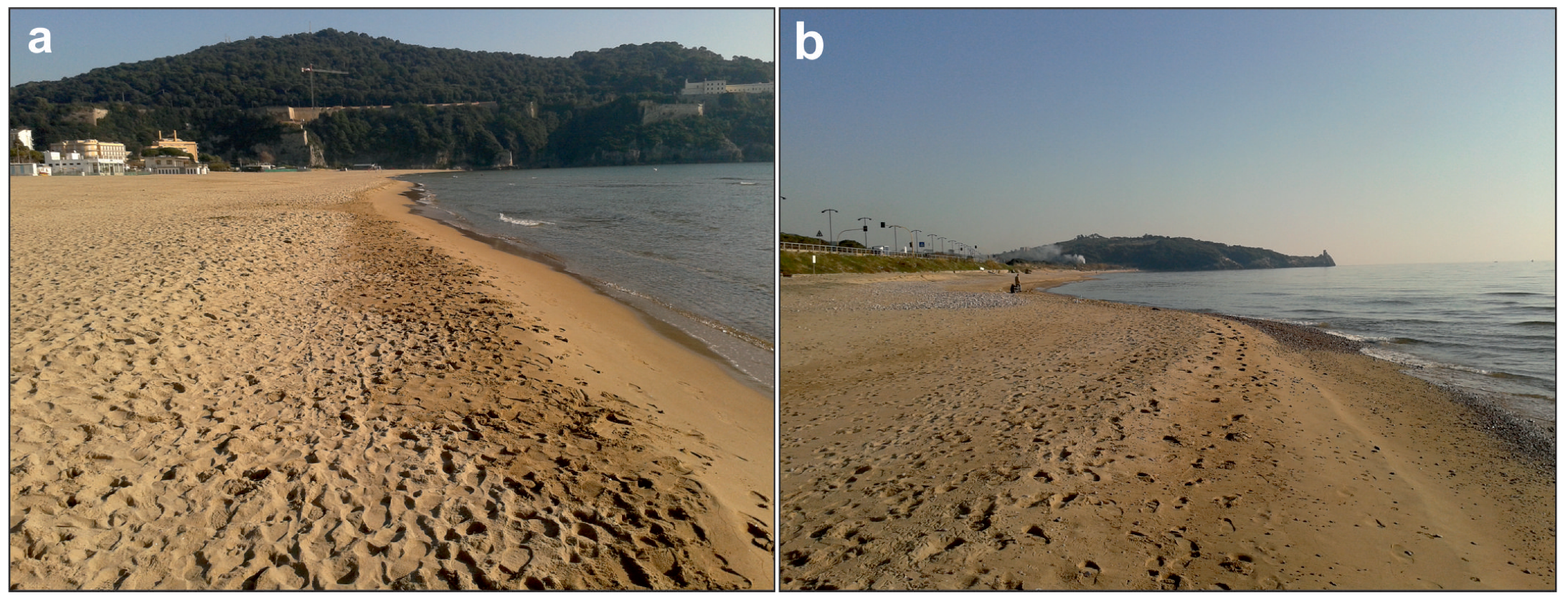
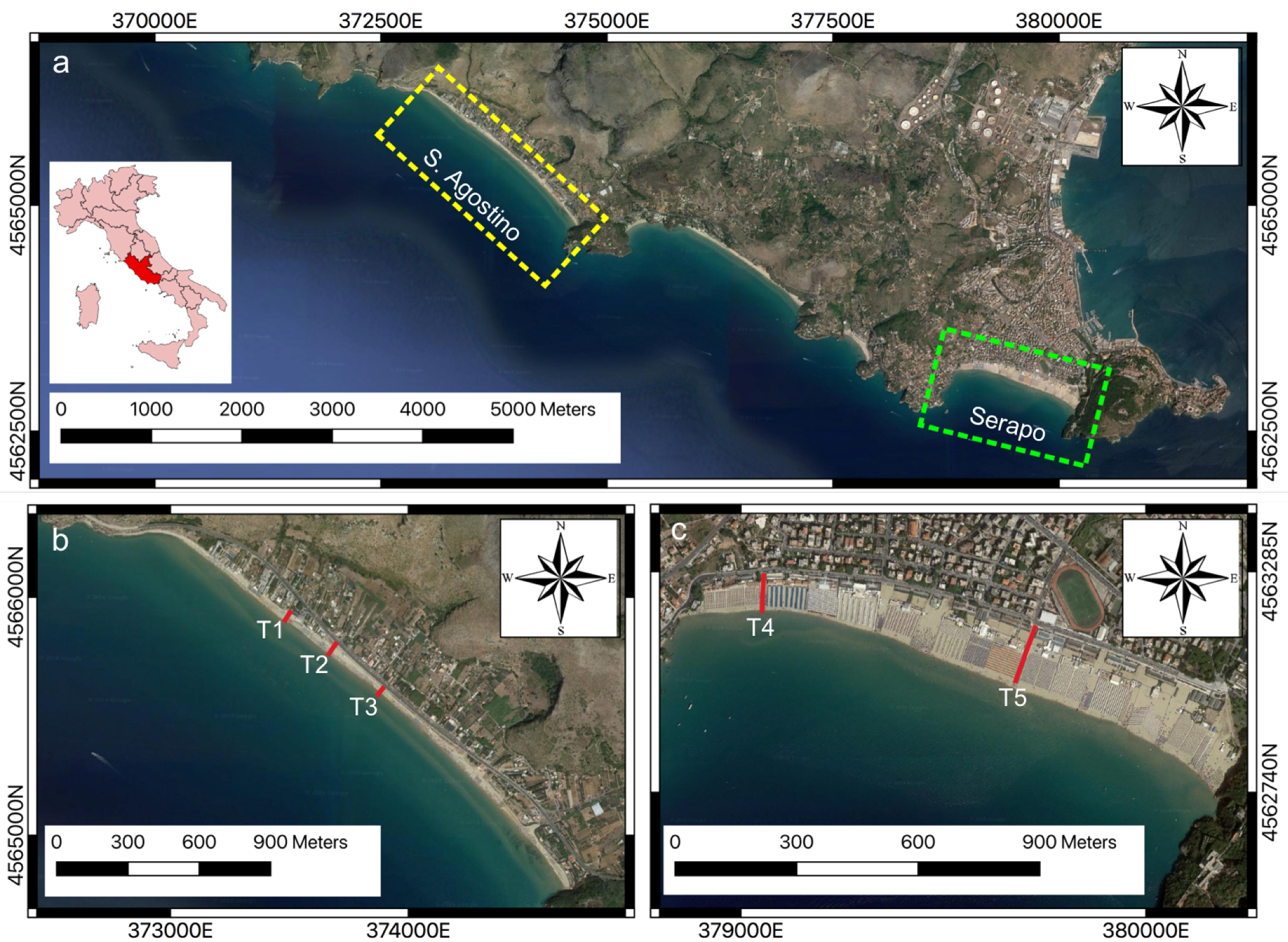
2. Study Area

The study area is in the central Tyrrhenian Sea (Italy) (Figure 1a), in the municipality of Gaeta (LT). Gaeta is a town with about 20,000 residents, which nearly triplicate during the summer season, since the town is a touristic destination for summer holidays. Consequently, in this area the pressures on the coast are high: in some parts of the territory, infrastructures and bathing facilities are located less than 50 m from the shoreline. This coastline sector, from the headland of Monte Orlando (41°12${}^{\prime }$28.03${}^{″}$ N, 13°34${}^{\prime }$33.83${}^{″}$ E) northwards to Torre Capovento (41°14${}^{\prime }$22.99${}^{″}$ N, 13°28${}^{\prime }$17.97${}^{″}$ E), is characterized by a succession of rocky calcareous headlands and sandy beaches developed in embayments connected to structural lines, transversal to the coastline. This configuration (alternation of large and small embayed beaches) is also related to the presence of NE-SW oriented faults, as well as cliffs, whose development was controlled by tectonics [32]. In detail, the beaches of Serapo and S. Agostino (Figure 1b,c) are considered. Serapo beach has a length of approx. 1.45 and with 64 bathing facilities is the main beach of Gaeta. S. Agostino beach, with approx. 2.2 km of coastline, is the longest beach of Gaeta.

3. Methodology

3.1. Beach Characterization and Shoreline Detection

The shoreline detection was performed by using different techniques. Following Manno et al. [33], we considered a time-history through the available aerial images of the study area, completed by a DGPS (Differential Global Position System) RTK (Real Time Kinematic) survey. Moreover, the geomorphological characterization is based on 5 beach profiles, realized by using DGPS analysis. Furthermore, several samples were collected along each profile in the backshore and foreshore zones, to describe the sedimentary features of these beaches. In detail, the grain size analysis (medium value of the particle size distribution $\mu$) was carried out by applying the ASTM international standard D421 and D422 [34,35] and the Wentworth scale.

3.1.1. Orthophoto Processing

The most common shoreline detection technique applied to visibly discernible shoreline features is manual visual interpretation, either in the field or from aerial photography [36]. Manual identification relies on the individual skills of the interpreter, according to Anders and Byrnes [37] and Byrnes et al. [38] and often may require the operator to be familiar with the investigated shore. HWL (High-Water Line) methods were adopted to identify the wet/dry boundary, which is determined as a change in tone left by maximum run-up from a preceding high tide, according to Crowell et al. [39] and Del Río et al. [40]. HWL visual interpretation was used to evaluate medium term coastline changes, employing an aerial photograph and three orthophotos dating from 1954 to 2008, at scales of 1:10,000 and 1:33,000. The aerial shooting of the I.G.M. of the Regione Lazio dates to 1954 and covers the entire regional territory. Frames formed 23 × 23 at the approximate scale 1:33000 were performed with the machine socket FAIRCHILD equipped with a lens with focal length 153.89 mm. 2000, 2006 and 2008 orthophotographs, at a scale of 1:10000, were provided by the Italian Ministry for Environment, Land and Sea Protection. The used image dataset was available on http://www.pcn.minambiente.it (last access: 1 April 2018) and on the Regione Lazio Geoportal.

3.1.2. DGPS Surveys

The present-day beach morphology and the 2018 shoreline position were investigated through topographic measurements carried out by means of a DGPS-Trimble R6) characterized by very high accuracy (Root Mean Square Error − RMSE = ±0.3 m). In detail, 5 beach profiles (Figure 1) were traced orthogonally to the shorelines of the Serapo and S. Agostino beaches starting from their inner limit or the crest of the dunes to an elevation of $-1.0$ m a.s.l. in the offshore direction. The shoreline was obtained through an RTK survey, assessing the shoreline position identified as the high-water line [41,42,43] on the beaches. The shoreline position was calibrated considering a micro-tidal excursion of ±20 cm (ISPRA, http://www.idromare.it/analisi_dati.php, last access: 10 October 2014).

3.2. Beach Rotation

The total shoreline variation extracted from remote sensing images and/or direct surveys was divided in two components: a translational movement of the shoreline in the cross-shore direction and a rotational movement around a pivotal point. Following Turki et al. [25], considering $P_n$ as the number n (equal to 14 for Serapo beach and equal to 22 for S. Agostino beach) of cross-shore profiles P, the total variation of their position in the time interval $\Delta$$P_n=P_n\left(t\right)-P_n\left(t_0\right)$, can be conceptually summarized as reported in Equation (1).

$$\Delta P_n\left(t\right)=M_{tr}\left(t\right)+M_{ro{t}_n}\left(t\right)$$

(1)

The translation movement $M_{tr}\left(t\right)$ is the same along the beach and it can be evaluated as reported in Equation (2).

$$M_{tr}\left(t\right)=\frac{1}{n}\sum _{i=1}^n{P}_n$$

(2)

The rotation movement $M_{ro{t}_n}\left(t\right)$ is different for each $P_n$ transect and can be evaluated as reported in Equation (3).

$$M_{ro{t}_n}\left(t\right)=\Delta P_n\left(t\right)-M_{tr}\left(t\right)$$

(3)

This approach approximates the real case study (represented by the beaches of Serapo and S. Agostino), in which the shoreline movements are more complex and often characterized by a rotation movement without a clear pivotal point located approximately on the central section of the beach, with beach retreat at one end and beach advance at the other.

3.3. UAV and SAR Remote Surveys for Coastline Evolution

To supplement the aerial and terrestrial photogrammetry, coastline extraction was obtained also by UAV images and dual-polarimetric SAR data.

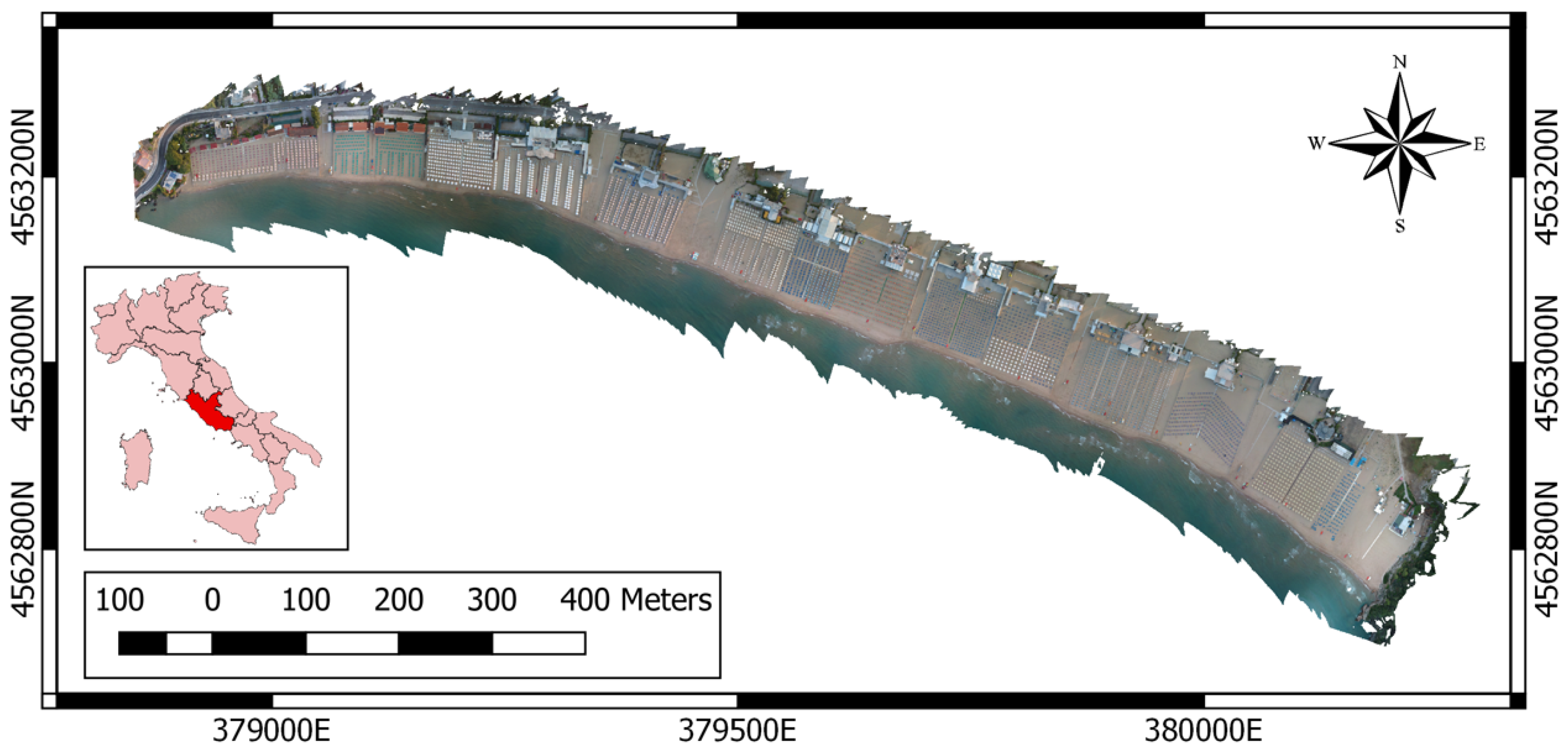
3.3.1. UAV Measurements

For coastline measurements, a UAV exacopter was used, weighing about 2500 g, carrying on board a GPS and a multidirectional accelerometer to ensure the beach survey through a sweep with constant speed, direction and altitude, each flight recording 500 to 800 shots. The height of flight was dictated by the spatial scale of the study area, and an altitude of 100 m was used. The on-board camera was a Canon 16 M pixels, with fixed and constant focal takeoff to perform the 3D cloud points. Six adjacent strips were performed for the survey realization with pictures taken every second in sequence, to allow a minimum overlap of 80%. A direct topographic site survey was performed with a Trimble R6 DGPS in RTK mode for the placement of GPS markers and georeferencing of the final product. The Digital Surface Model (DSM) of the micro-tidal beach was obtained to update to 2018 the erosional\accretional trends (reported in Figure 2), already detected by means of multi-temporal analysis and in situ GPS survey. The comparison between the UAV and the other in situ and remote surveys is reported in Section 4.

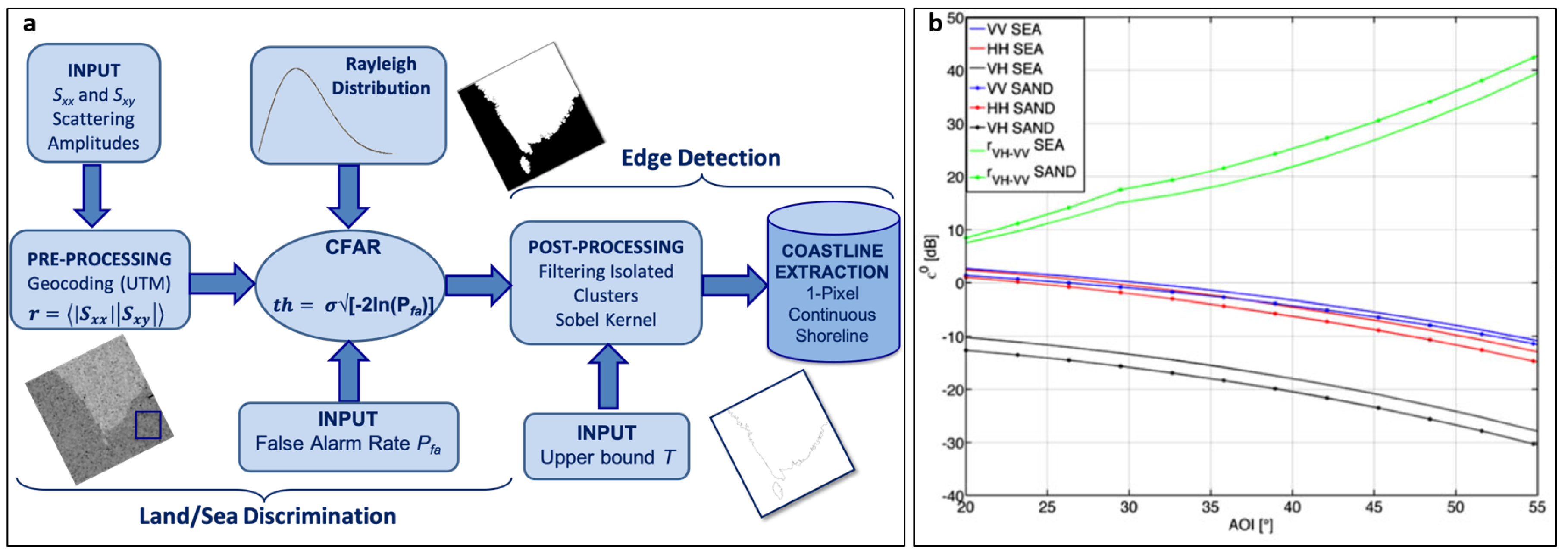
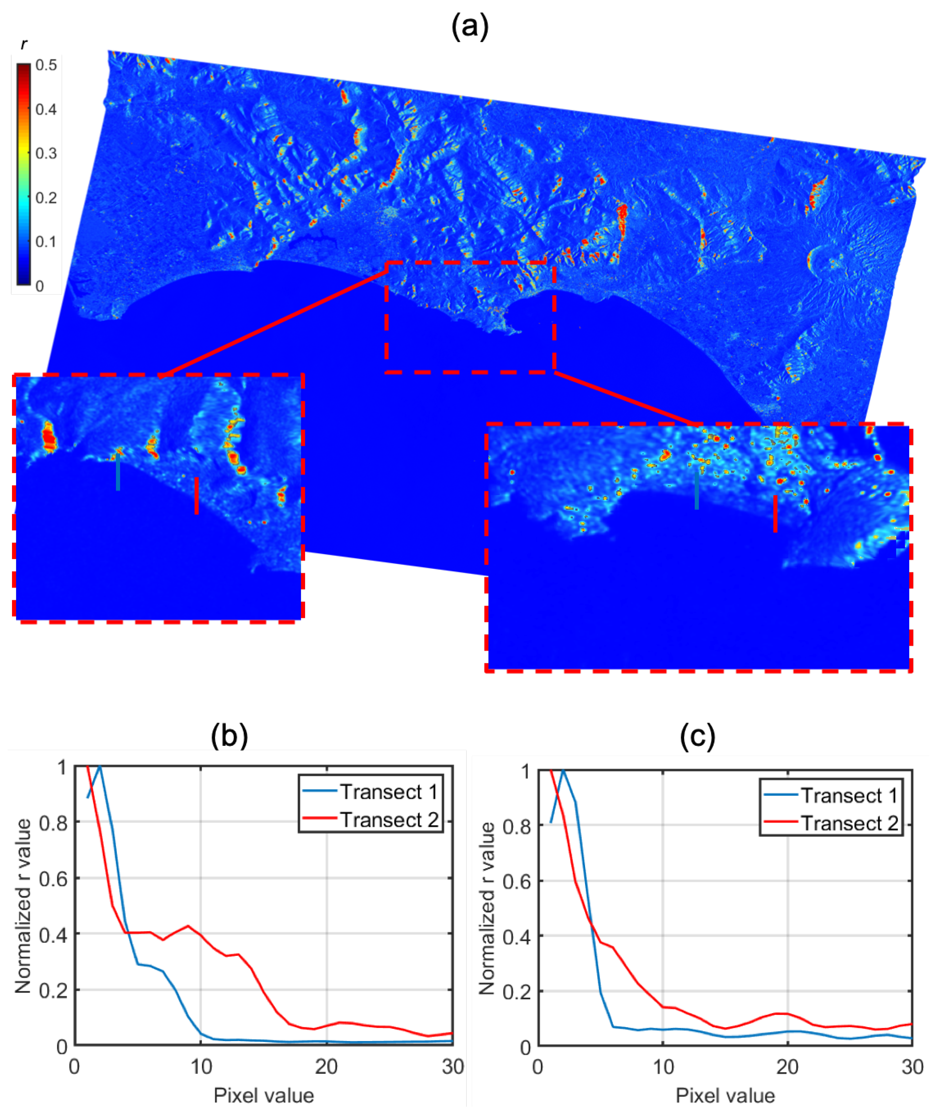
3.3.2. SAR Observations

Polarimetric SAR is an active coherent sensor that measures, for each resolution cell, two or more elements of the scattering matrix S. The latter is a $2\times 2$ matrix of complex elements, termed as scattering amplitudes, that describes the relationship between the incident linearly polarized (along horizontal—H—or vertical—V—direction in a plane orthogonal to the propagation direction) electromagnetic wave transmitted by the sensor and received by the SAR antenna, in a linearly polarized H-V basis, once it was scattered off the observed scene. In the backscattering case, S is given by:

$$\mathbf{S}=\left(\begin{array}{cc}{S}_{\mathrm{HH}}& S_{\mathrm{HV}}\\ S_{\mathrm{VH}}& S_{\mathrm{VV}}\end{array}\right)$$

(4)

In the backscattering case and assuming reciprocity, i.e., |$S_{\mathrm{HV}}$| = |$S_{\mathrm{VH}}$|, S consists of five independent real quantities (i.e., the modulus of the three scattering amplitudes and the relative phase between the co-polarized channels and between co- and cross-polarized channels). When natural scattering surfaces are observed, the reflection symmetry property is satisfied that results in co- and cross-polarized channels being uncorrelated, i.e., the phase information is uninformative [5,44].

When dealing with polarimetric SAR sensors, different imaging modes are available. In this study, a dual-polarimetric SAR, i.e., the one that transmits a single polarization (e.g., vertical—V) while receiving simultaneously according to an orthogonal linear polarization basis (e.g., H and V), is considered. It must be pointed out that in this case, only a subset of polarimetric information is available, i.e., a single row of the scattering matrix is measured if compared to quad-polarimetric SAR imaging modes that measure the complete scattering matrix. Nevertheless, the latter costs in terms of limited swath width, reduced AOI (Angle Of Incidence) range and more demanding hardware constraints and, therefore, the dual-polarimetric SAR mode is here exploited that was shown to be effective in shoreline extraction [5,45,46].

In this study, shoreline extraction is performed according to the metric r proposed in [5]. The latter exploits the dual-polarimetric co- and cross-polarized information as follows:

$$r=\langle \left|S_{\mathrm{VV}}\right|\left|S_{\mathrm{VH}}\right|\rangle$$

(5)

where $|·|$ and $\langle ·\rangle$ stand for modulus and ensemble average, respectively. Please note that in this study, the ensemble average is replaced by spatial averaging undertaken using a 9 × 9 boxcar filter, as suggested in [5]. This metric, as shown in [5] through Improved Integral Equation Method (IIEM) model-based simulations, is expected to increase sandy land/sea separation with respect to the single-channels intensity information in a robust and effective way, see Figure 3b.

Once r is obtained according to Equation (5), a binary output where land and sea are clearly separated is provided, in an unsupervised way, by means of a global threshold generated following a Constant False Alarm Rate (CFAR) approach. The latter relies on the fact that the r parameter follows a Rayleigh statistical distribution, see [5]. Once the binary image is provided, isolated groups of pixels at sea (e.g., metallic targets, small islands, etc.) that consist of less than a given number of pixels (selected according to both the SAR sensor’s spatial resolution and the typical size of the targets to be filtered out) are sorted out. Then, a conventional edge detector, based on the Sobel kernel that was shown to be effective in performing a two-dimensional spatial gradient measurement on the binary output to emphasize edges, is applied to extract the 1-pixel continuous shoreline [47]. The above-mentioned methodology was tested on a large dataset that include C- and X-band coherent and incoherent dual-polarimetric SAR imagery collected under different conditions (AOI, coastal morphology, sea state, etc.) and validated against actual GPS measurements [5,48]. At C-band, over challenging scenarios (i.e., sandy beaches and low-backscattering sea surface areas), the adopted methodology was shown to be accurate (a mean ± standard deviation distance of 4.6 ± 3.3 pixels between the extracted shoreline and GPS measurements is achieved) and time-effective (a few seconds to process a whole SAR image) [5]. The flowchart of the proposed approach is summarized in Figure 3a.

In this study, the 1-pixel continuous shoreline is extracted from a time series of 18 Sentinel-1 (S1) dual-polarimetric VV-VH ground range detected (GRD) SAR scenes collected in Interferometric Wide (IW) swath mode from October 2014 to November 2018 over the study area that includes part of the gulfs of Naples and Gaeta, with the latter hosting the Serapo and S. Agostino beaches.

The S1 IW mode provides moderate spatial resolution measurements (5 m × 20 m along range and azimuth directions, respectively) over a very wide swath of about 250 km. The IW mode captures three sub-swaths using Terrain Observation with Progressive scans SAR (TOPSAR), each of which consists of several bursts that result in a wide AOI range spanning from about 30${}^{\circ }$ up to approximately 46${}^{\circ }$. An overview of the considered S1 SAR dataset is listed in

Table 1. Sentinel-1 SAR data set.

Number of Scenes	Acquisition Period	Band	Polarization	AOI (${}^{\circ }$)	Swath (km)	Pixel Spacing (m)
18	October 2014–November 2018	C	Dual-pol IW (VV-VH)	30–46	250	10

, while additional information on the S1 SAR imaging characteristics can be found in [49].

Among the whole SAR dataset, results relevant to the SAR scene collected on June 2018, processed according to the above-mentioned methodology, are presented and discussed as a showcase. First, radiometric calibration and UTM (Universal Transverse Mercator) reprojection using a 10 m pixel spacing is applied as a pre-processing step.

Then, the r image is obtained according to Equation (5), see Figure 4a, where the areas relevant to the Serapo and S. Agostino beaches are highlighted by two Regions Of Interest (ROIs) marked by red dashed boxes. It can be noted, as expected, that r values over sea surface are very close to 0 while, over land, quite larger r values apply. A quantitative analysis on the behavior of r over both sea and sandy beaches is undertaken along a pair of 30-pixels long transects selected in the cross-shoreline direction over both ROIs, see red and blue lines in Figure 4a. The behavior of r, normalized with respect to its maximum value, along the selected transects is shown in Figure 4b,c for Serapo and S. Agostino beaches, respectively. In both cases, it can be observed that r values over land are almost an order of magnitude larger than the corresponding values over sea surface. Nonetheless a transition region, which is about 5 to 10 pixel-long, between land and sea is observed, where normalized r values decrease from ≈1.00 on sandy land down to ≈$0.05-0.010$ on sea surface, with the sharpness and rapidity of the decreasing trend being closely related to the beach morphology (and, therefore, to the given transect). Then, a global threshold for the whole SAR scene is obtained according to the CFAR approach (see Figure 3a), where $P_{fa}$ = ${10}^{-6}$ is set. Once the binary image is provided, the removal of isolated clusters of T = 500 pixels at sea is performed as a post-processing step. Hence, after Sobel kernel edge detection, the 1-pixel continuous shoreline is finally extracted.

4. Results

4.1. Beach Characterization

The S. Agostino and Serapo beaches present a rather regular morphology and rectilinear shorelines (Figure 5), aligned respectively in the NW-SE and WNW-ESE direction. Their main morpho-sedimentary features are synthetically reported in

Table 2. Summary of main morpho-sedimentary characteristics of beaches profiles.

Profiles	Beach	Dune Ridge Height [m]	Backshore Beach Width L [m]	Backshore Beach Slope ${\mathit{m}}_0$ [%]	Foreshore Beach Slope $\mathit{\beta }$f [%]	Backshore Beach $\mathit{\mu }$ [mm]	Foreshore Beach $\mathit{\mu }$ [mm]
T1	S. Agostino	-	24.4	6.6	15.5	0.378	0.376
T2		-	26.6	4.5	24.4
T3		-	17.9	5.1	16.1
T4	Serapo	2.8	57.8	2.5	18.2	0.381	0.376
T5		2.4	81.7	1.5	11.1

by with reference to profiles T1–T3 for S. Agostino and T4–T5 for Serapo (for location see Figure 1). The study beaches are limited by carbonate headlands at their extremities that isolate the beaches with respect to the possible import and export of sediments due to long-shore currents. Beach sediments are characterized by homogenous grain size features both in the foreshore and backshore sectors, with grain sizes between 0.376 mm and 0.381 mm (Table 2) indicating medium sands. Beach widths are rather variable highlighting notable differences between the two. The smaller S. Agostino beach has widths comprised between 17 and 30 m, typically around 20 m in its central sector (17.9 m to 24.4 m, see Table 2). The Serapo beach is much larger being characterized by minimum and maxim widths of respectively 50 and 130 m, and values typically around 60–80 in its central portion (57.8 and 81.7 m profiles T4 and T5 in Table 2). According to the differences in width of the beaches, backshore slopes are significantly higher along the S. Agostino beach (between 4.5 and 6.6%, Table 2) than along the Serapo beach (between 1.5 and 2.5%, Table 2).

Both beaches have low elevations, generally under 2 m a.s.l., with maximum heights measured for the Serapo beach in correspondence of some local residuals of dune cover (2.8 m and 2.4 m a.s.l., profiles T4 and T5 respectively, Table 2).

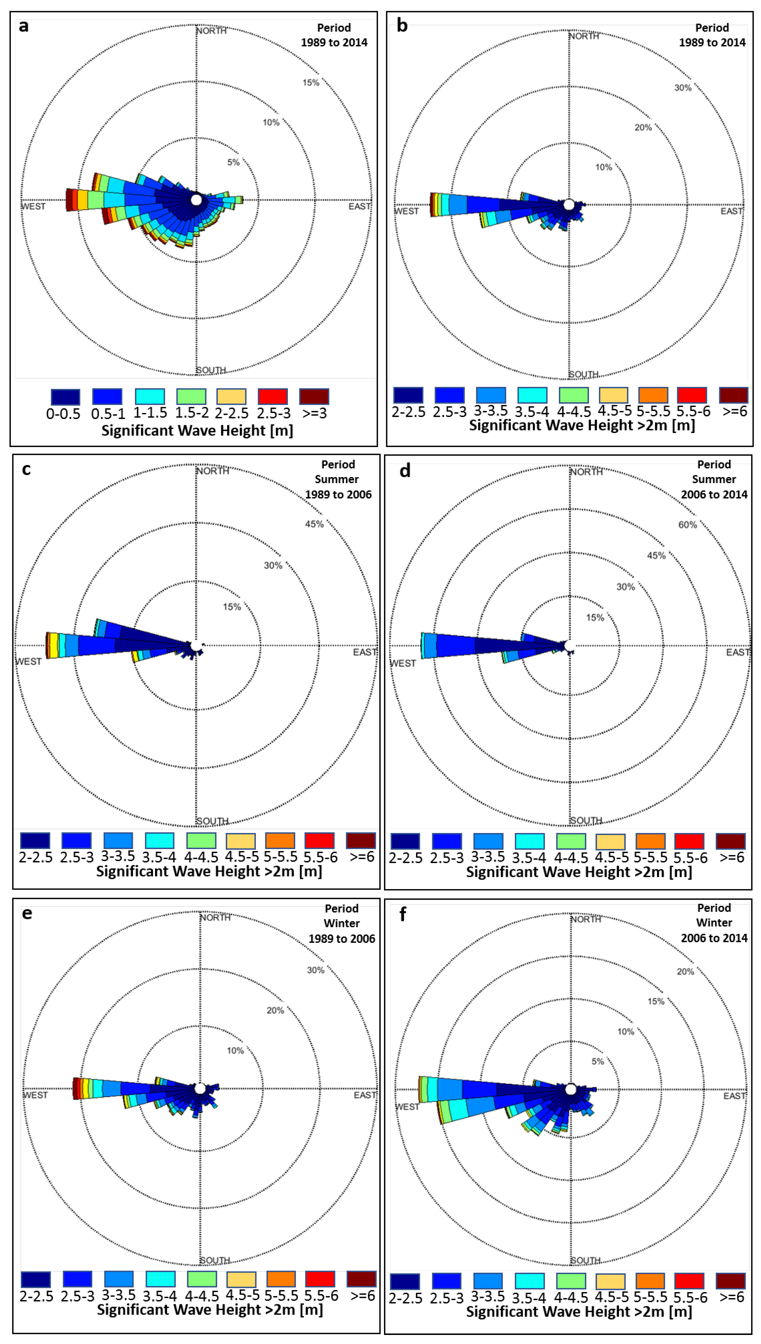
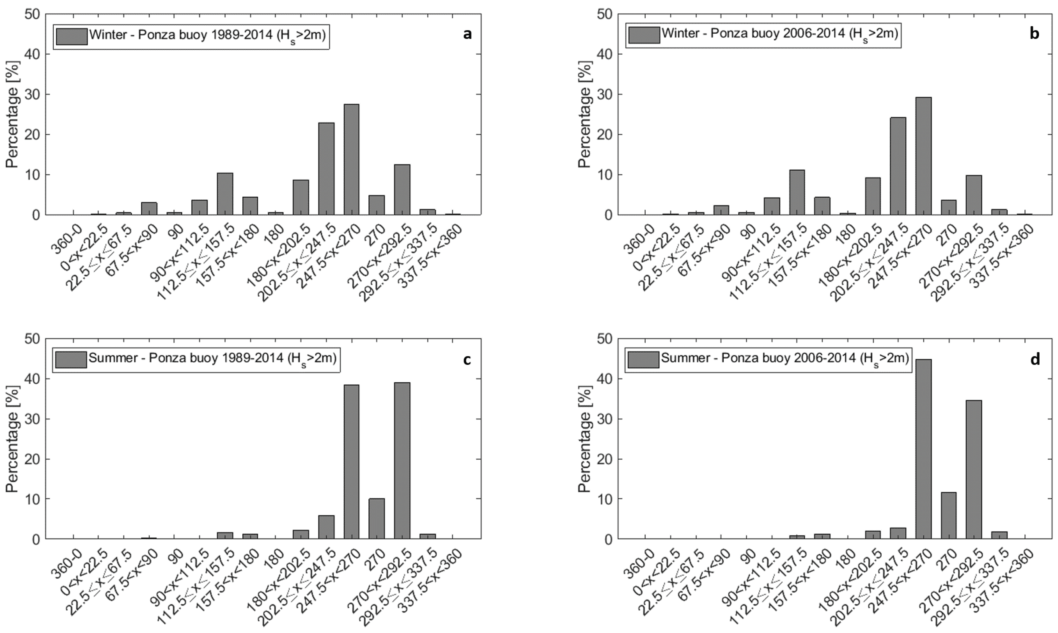
4.2. Wave Climate

To evidence the possible link between the shoreline evolution and the wave climate that affects the study area, we analyzed the wave data provided by the Italian Sea Wave Measurement Network [50] through the records of the Ponza buoy (40°52${}^{\prime }$00.10${}^{″}$ N, 12°56${}^{\prime }$60.00${}^{″}$ E) during the period July 1989–December 2014 (a total of 12,766 wave records including significant wave height $H_s$, mean wave period $H_m$ and mean wave direction $D_m$). In Figure 6 we reported the directional distribution for the entire period covered with the data (1989–2014), with reference to all $H_s$ (a) and to $H_s$ higher than 2 m (b). Moreover, a seasonal distribution of the highest waves is reported for the periods 1989–2006 (see (c) for summer and (e) for winter) and 2006–2014 (see (d) for summer and (f) for winter). A visual inspection of Figure 6c–f shows that there are no appreciable differences between the wave directional distribution in the first and in the second period during the winter, while in the summer season a slightly higher percentage of waves coming from the third quadrant and a lower percentage of waves coming from the fourth quadrant can be appreciated. This result is even more evident in Figure 7, which reports the bar diagram of directional occurrence of $H_s\ge 2$ m for the winter season with reference to the entire dataset (a) and 2006–2014 dataset (b); for the same periods we reported the diagrams relative to sea states occurring during the summer seasons in (c,d), respectively. The result of the seasonal analysis shows that in winter the study area is affected by wave conditions associated with $H_s\ge 2$ m coming from both sectors SSE and WSW (Figure 7a,b), while in summer only the waves coming from WSW remain (Figure 7c,d). Moreover, the comparison between the entire dataset and the most recent one shows no difference for the winter season, while in the summer season we detect more waves coming from W (from 40% to 45%) and less waves coming from NW (from 40% to 35%). The bar diagrams show that the directional distribution of $H_s$ has varied in the summer season in recent years, with a higher percentage of waves coming from W and a lower percentage of waves coming from the NW. The beaches examined are less sheltered from the first storms, whose increased percentage causes a partial flow of sediments from the western to the central and eastern areas of the two beaches.

4.3. Shoreline Evolution

As detailed in methods, the evolution of the coastline was reconstructed by a multi-temporal analysis taking in consideration aerial images and in situ measurements. The graphical results of the shoreline evolution are reported in Figure 8a,b for the beaches of Serapo and S. Agostino, respectively, while the related numerical results in terms of translation and rotation movements are given in Figure 9 and Figure 10.

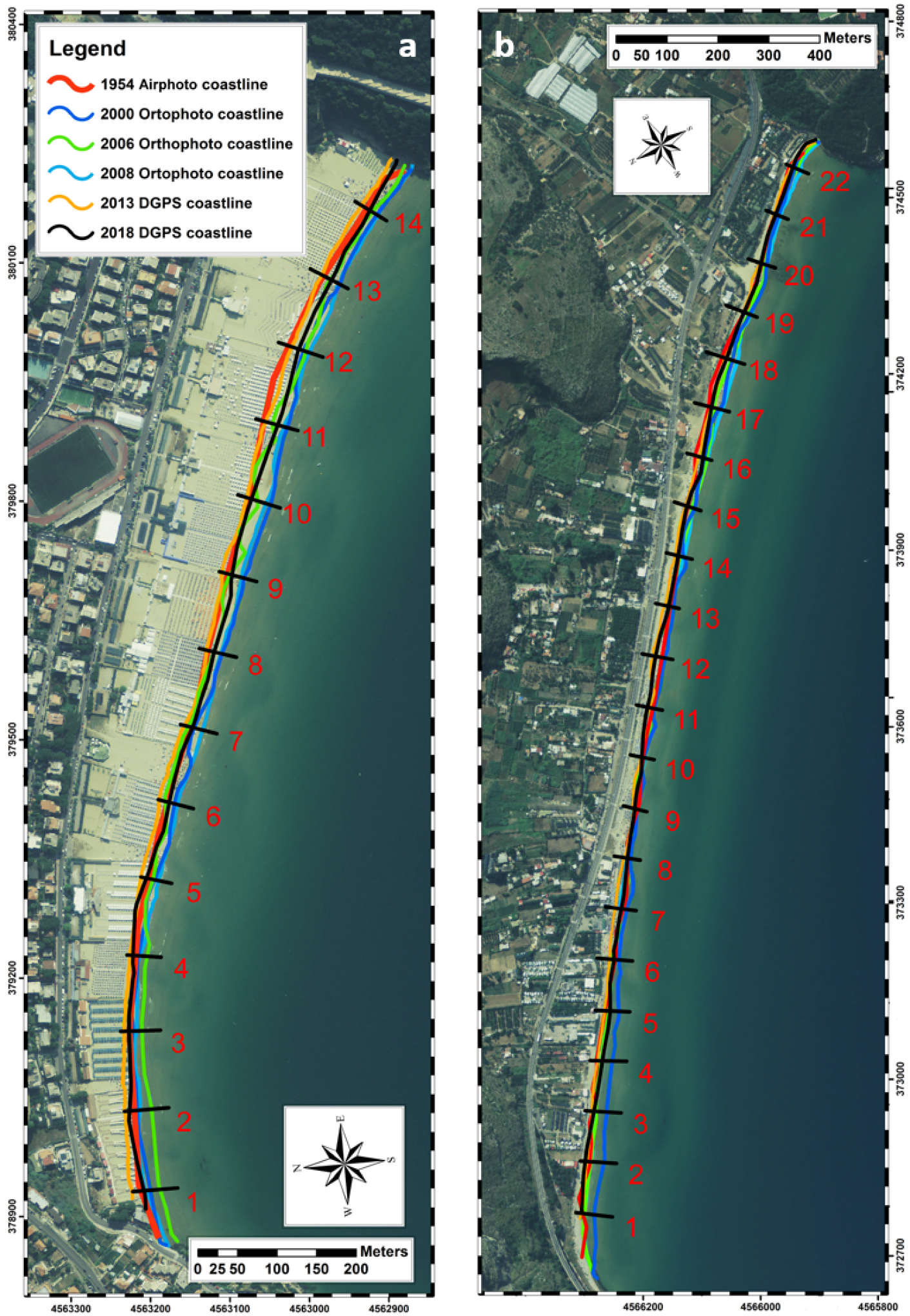
4.3.1. Serapo Beach

The shoreline variations were evaluated along 14 transects, spaced 100 m apart. Given the orientation of the shoreline (WNW-ESE), two sectors, western and eastern, are distinguished. The results are as follows:

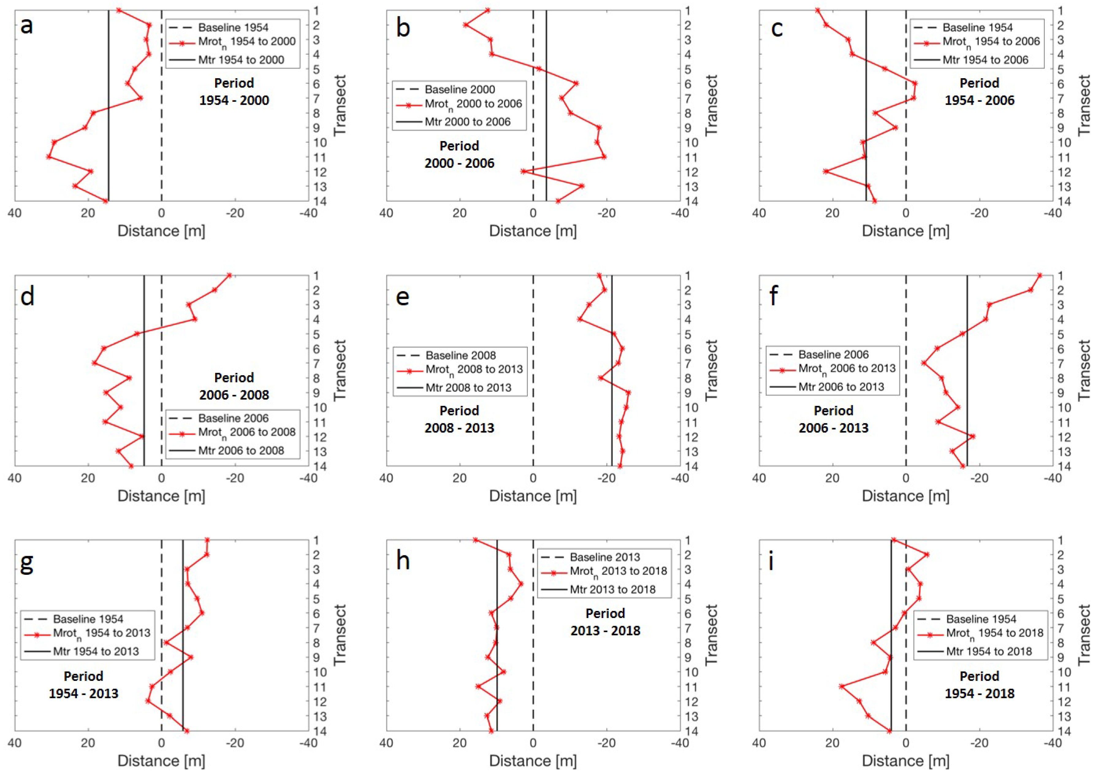
• 1954–2006 (52 years).
  Figure 8a shows a generalized beach advance, with a maximum in 2006 (green line), particularly for the western and eastern extremities.
  1954–2000 (Figure 9a): An inhomogeneous shoreline advance of between a few meters in the western to approx. 30 m in the eastern sector affects the beach.
  2000–2006 (Figure 9b): The western sector clearly advances, while the eastern sector retreats. This coincides with an anticlockwise rotation of the beach around a virtual pivotal point near transect 5.
  1954–2006 (Figure 9c): The overall result for this period is the sum of the precedent, contrasting ones, i.e., a moderate increase in the beach width in both the western and eastern sectors.
• 2006–2013 (8 years).
  2006–2008 (Figure 9d): A consistent erosion affects the western sector (max. ca. 18.5 m, transect 1), contrasting a progradation of up to 18 m in the eastern sector. A clockwise rotation of the beach around virtual pivotal point located near transect 5 occurs.
  2008–2013 (Figure 9e): rather homogeneous retreat affects the entire coast, with values comprised between about 10 and 25 m, slightly more intense in the eastern sector.
  2006–2013 (Figure 9f): A significant erosion of the entire beach occurs, with maximum values of more than 30 m in the western sector and around 15 in the eastern sector. In the central part of the beach shoreline retreat is more modest, max. 10–11 m (transects 6–9).
• 1954–2018 (62 years). The graphical result given in Figure 8a shows a general beach recovery, more significant for the eastern sector, in which the 2018 coastline (black line) is more detached from the 2013 coastline (yellow line). Figure 9 again confirms this result, with the evolution 2013–2018 reported in (h).
  1954–2013 (Figure 9g): This period sums up the two previous major periods 1954–2006 and 2006–2013 (Figure 9c,f). The result is a slight retreat of the western sector, and some small advance of part of the eastern sector that “preserves” part of the clockwise rotation occurred in 2006–2008.
  2013–2018 (Figure 9h): There is a moderate and irregular beach recovery with values of 5 to 15 m, slightly more consistent in the eastern sector.
  1954–2018 (Figure 9i): The overall result is a net clockwise rotation of the beach around a central virtual pivotal point (transect 7), with an overall slight shoreline retreat in the western sector (max. values around 5 m) and a net, although irregular progradation of the eastern sector.

4.3.2. S. Agostino Beach

The shoreline variations were evaluated along 22 transects, spaced 100 m apart. Given the orientation of the shoreline (NW-SE), two sectors, north-western and south-eastern, are distinguished.

The results are as follows:

• 1954–2006 (52 years).
  Figure 8b shows the stability of the whole beach due to an advance in 2000 (blue line) followed by a retreat in 2006 (green line).
  1954–2000 (Figure 10a): A consistent shoreline advance affects the beach extremities with maximum values of 20–30 m in the north-western sector (transects 1–5).
  2000–2006 (Figure 10b): Retreat affects nearly all the beach, more pronounced in the north-western sector (max. values of 30 m). An initial clockwise rotation of the beach is the result.
  1954–2006 (Figure 10c): The beach has advanced along the extremities, especially in the south-eastern sector with max. values of ca. 20 m.
• 2006–2013 (8 years).
  2006–2008 (Figure 10d): The beach slightly retreats in the north-western sector, and advances in the south-eastern sector. A slight clockwise beach rotation is the result.
  2008–2013 (Figure 10e): A retreat of the entire beach occurs, much more pronounced in the south-eastern sector. The result is a slight anticlockwise rotation with a virtual point located in the central part of the beach.
  2006–2013 (Figure 10f): The sum of the two contrasting precedent shoreline rotations is an overall shoreline retreat, more intense in the south-eastern sector.
• 1954–2018 (62 years).
  The inspection of Figure 8b does not help to identify a clear trend.
  1954–2013 (Figure 10g): The beach is stable along the extremities and retreats in the central part.
  2013–2018 (Figure 10h): There is some irregular beach recovery with maximum values around 10 m.
  1954–2018 (Figure 10i): The beach is globally stable, the base line in 2018 practically coincides with that of 2018.

In synthesis, comparing the two beaches the following outcomes can be highlighted: Regarding the period 2000–2013, both the beaches have experienced clockwise and anticlockwise rotations. Regarding the entire time window 1954–2018, both the beaches, keeping in mind their critical conditions during the 1980s highlighting a net trend to shoreline retreat (www.comune.gaeta.lt.it/content/download/4432/26368, last access: 10 January 2019), have entirely recovered (S. Agostino) or partially even advanced (eastern sector of Serapo). Furthermore, a global trend of beach rotation can be defined for the Serapo beach, while the contrasting rotations of the S. Agostino beach have cancelled single effects, whereby no global trend is evident.

4.4. Validation of UAV and SAR Remote Surveys with DGPS

In this subsection, shoreline extraction over the study area from UAV and SAR data is validated by means of DGPS measurements.

The comparison between DGPS, UAV and SAR shoreline extracted during summer 2018 is reported in Figure 11, where the actual shoreline positions are depicted in yellow for the SAR (30 June 2018), in green for the DGPS (28 June 2018) and in red for UAV (9 July 2018). It can be observed that UAV extracted coastlines fit the actual DGPS coastal profile quite well. When dealing with coastlines derived from DGPS and UAV, they are almost overlapped, even though beach extremities are quite different (maximum variation = 2.5 m), due to the different tidal range (approximately 0.15 cm between the DGPS and UAV surveys) and lowest beach slopes at the beach extremities (5–10%).

When dealing with SAR-based shoreline extraction, results are severely affected by the limited spatial resolution (in this case, 1 pixel corresponds to 10 m). However, the extracted shoreline follows the coastal profile along the whole beach, even though a shift towards the sea can be observed. Nevertheless, it must be pointed out that satellite polarimetric SARs represent a time- and cost-effective solution for long-term coastline detection on a large spatial scale.

5. Discussion

In this study, we investigated the mid-term shoreline evolution of two embayed beaches located along the central Tyrrhenian coast of Italy. Our analysis has been carried out by means of airphotos, orthophotos, UAV, SAR and DPGS surveys. The analysis highlighted a different behavior exhibited by the two beaches. The global evolution 1954–2018 of Serapo beach highlights a rotation around a virtual pivotal point, a retreat in the west and an advance in the east. The beach of S. Agostino has remained on overall stable, and it is not possible to identify an equally defined beach rotation. The reason for this difference can be attributed to several conditions, mainly beach orientation. For Serapo beach the significant angular difference between the wave orthogonal and the beach normal gives rise to a local long-shore current directed from the western limit to the central part, while for S. Agostino beach this angular difference decreases, and the beach is apparently more subjected to cross-shore transport. The results show that changes in the wave directional distribution during summer can be responsible for the observed beach rotation around a pivotal zone. These results agree with the ones of Turki et al. [25] who correlated the rotation and translation of the beach with the cross-shore and long-shore component of the energy flux. Instead, we could not made correlations between wave and shoreline data, for the lack of wave records inside the bays, which, we hope, will be the subject of future research. Moreover, a more detailed a seasonal shoreline evolution could be obtained using a continuous beach video-monitoring system as proposed by Harley et al. [51] to monitor the shoreline dynamic of gravel embayed beach in Central Italy. Most recent shoreline changes and related rotations cannot be evidenced with the aid of SAR tools since the SAR-based extracted coastline is shifted towards the sea of about 20–30 m, likely due to the inherent SAR imaging process (i.e., speckle noise) together with sea state/coastal morphology conditions (i.e., tidal and bathymetry effects) as already observed in [5,46,52,53,54], respectively. In [46], it was suggested that this shift is mainly related to the combination of SAR imaging characteristics as AOI and incident wavelength, with environmental conditions including bathymetry and coastal slope.

Nonetheless, even though those effects reduce the land/sea contrast introducing errors in the accurate determination of the actual shoreline position, this shift falls within the accuracy achieved by the proposed methodology (about 4 pixels on average) if the actual pixel size is taken into account [5]. In addition, it must be stressed that in case of long-term analysis of coastal erosion/accretion processes, the shift experienced by the shoreline extracted from SAR imagery represents a bias that may affect the whole time series in the same way, without affecting the analysis of global trends. Anyway, it was shown that the exploitation of quad-polarimetric information or the availability of finer resolution polarimetric SAR imagery can reduce this bias, although at the expense of area coverage and hardware complexity [48].

6. Conclusions

The analysis of the coastline evolution of the beaches of Serapo and S. Agostino has highlighted a partial rotation of the first and more complex variations of the second one, with the result of an overall stability of the shoreline by considering the entire time interval investigated (1954–2018). We explained this behavior with a different directional wave distribution in more recent years, consisting of a greater percentage of waves coming from W and a lower percentage of waves coming from NW in the summer season. The reason for this behavior is probably due to a different shoreline orientation. These results were obtained by shoreline extraction from airphotos, orthophotos and conventional in situ DGPS surveys, because the resolution of polarimetric SAR imagery is not yet adequate. Nevertheless, the results given by polarimetric SARs are complementary monitoring tools of shorelines in embayed beaches due to its non-cooperative and cost-effective capabilities to observe very large coastal areas. In addition, the data continuity guaranteed by space agencies through follow-on missions makes and will make available polarimetric SAR measurements over decades.

Hence, an integrated approach between different remote sensing tools investigated in this study to monitor shoreline rotation of embayed beaches is suggested that combines continuous and updated long-term remote sensing observations, together with in situ UAV, video-camera system and GPS measurement campaigns. Using the findings of this work, we are confident that we can implement our shoreline measures with modeling scenarios (i.e., nearshore wave model simulations or sediment transport) using GPGPU [55,56]-based high-performance cloud computing [57] as already done with sea pollutant transport and diffusion [58] and wave run-up forecast [8].

References

- Small, C.; Nicholls, R.J. A global analysis of human settlement in coastal zones. JSTOR 2003, 19, 584–599. [Google Scholar]
- Pikelj, K.; Ružić, I.; Ilić, S.; James, M.R.; Kordić, B. Implementing an efficient beach erosion monitoring system for coastal management in Croatia. Ocean Coast. Manag. 2018, 156, 223–238. [Google Scholar] [CrossRef]
- Guariglia, A.; Buonamassa, A.; Losurdo, A.; Saladino, R.; Trivigno, M.L.; Zaccagnino, A.; Colangelo, A. A multisource approach for coastline mapping and identification of shoreline changes. Ann. Geophys. 2006, 49, 295–340. [Google Scholar]
- Alesheikh, A.A.; Ghorbanali, A.; Nouri, N. Coastline change detection using remote sensing. Int. J. Environ. Sci. Technol. 2007, 4, 61–66. [Google Scholar] [CrossRef] [Green Version]
- Nunziata, F.; Buono, A.; Migliaccio, M.; Benassai, G. Dual-polarimetric C-and X-band SAR data for coastline extraction. IEEE J. Sel. Top. Appl. Earth Obs. Remote Sens. 2016, 9, 4921–4928. [Google Scholar] [CrossRef]
- Benassai, G.; Aucelli, P.; Budillon, G.; De Stefano, M.; Di Luccio, D.; Di Paola, G.; Montella, R.; Mucerino, L.; Sica, M.; Pennetta, M. Rip current evidence by hydrodynamic simulations, bathymetric surveys and UAV observation. Nat. Hazards Earth Syst. Sci. 2017, 17, 1493–1503. [Google Scholar] [CrossRef] [Green Version]
- Brignone, M.; Schiaffino, C.F.; Isla, F.I.; Ferrari, M. A system for beach video-monitoring: Beachkeeper plus. Comput. Geosci. 2012, 49, 53–61. [Google Scholar] [CrossRef]
- Di Luccio, D.; Benassai, G.; Budillon, G.; Mucerino, L.; Montella, R.; Pugliese Carratelli, E. Wave run-up prediction and observation in a micro-tidal beach. Nat. Hazards Earth Syst. Sci. 2018, 18, 2841–2857. [Google Scholar] [CrossRef]
- Aarninkhof, S.G.J. Nearshore Bathymetry Derived from Video Imagery; Delft University Press: Delft, The Netherlands, 2003. [Google Scholar]
- Turner, I.L.; Aarninkhof, S.; Dronkers, T.; McGrath, J. CZM applications of Argus coastal imaging at the Gold Coast, Australia. J. Coast. Res. 2004, 34, 739–752. [Google Scholar] [CrossRef]
- Holman, R.A.; Stanley, J. The history and technical capabilities of Argus. Coast. Eng. 2007, 54, 477–491. [Google Scholar] [CrossRef]
- Di Paola, G.; Aucelli, P.P.C.; Benassai, G.; Rodríguez, G. Coastal vulnerability to wave storms of Sele littoral plain (Southern Italy). Nat. Hazards 2014, 71, 1795–1819. [Google Scholar] [CrossRef]
- Benassai, G.; Di Paola, G.; Aucelli, P.P.C. Coastal risk assessment of a micro-tidal littoral plain in response to sea level rise. Ocean Coast. Manag. 2015, 104, 22–35. [Google Scholar] [CrossRef]
- Aucelli, P.P.C.; Di Paola, G.; Incontri, P.; Rizzo, A.; Vilardo, G.; Benassai, G.; Buonocore, B.; Pappone, G. Coastal inundation risk assessment due to subsidence and sea level rise in a Mediterranean alluvial plain (Volturno coastal plain–southern Italy). Estuar. Coast. Shelf Sci. 2017, 198, 597–609. [Google Scholar] [CrossRef]
- Di Luccio, D.; Benassai, G.; Di Paola, G.; Rosskopf, C.; Mucerino, L.; Montella, R.; Contestabile, P. Monitoring and Modelling Coastal Vulnerability and Mitigation Proposal for an Archaeological Site (Kaulonia, Southern Italy). Sustainability 2018, 10, 2017. [Google Scholar] [CrossRef]
- Short, A.; Masselink, G.E. Structurally Controlled Beaches. In Handbook of Beach and Shoreface Morphodynamics; Short, A.D., Ed.; John Wiley and Sons Ltd.: Chichester, UK, 1999; pp. 230–250. [Google Scholar]
- Da Fontoura Klein, A.H.; Benedet Filho, L.; Schumacher, D.H. Short-term beach rotation processes in distinct headland bay beach systems. J. Coast. Res. 2002, 18, 442–458. [Google Scholar]
- Martins, C.C.; de Mahiques, M.M.; Dias, J.M.A. Daily morphological changes determined by high-energy events on an embayed beach: A qualitative model. Earth Surf. Process. Landf. 2010, 35, 487–495. [Google Scholar] [CrossRef]
- Ojeda, E.; Guillén, J. Shoreline dynamics and beach rotation of artificial embayed beaches. Mar. Geol. 2008, 253, 51–62. [Google Scholar] [CrossRef]
- Bryan, K.; Gallop, S.; van de Lageweg, W.; Coco, G. Observations of rip channels, sandbar-shoreline coupling and beach rotation at Tairua Beach, New Zealand. In Coasts and Ports 2009: In a Dynamic Environment; Engineers Australia: Barton, Australia, 2009; p. 270. [Google Scholar]
- Short, A.; Cowell, P.; Cadee, M.; Hall, W.; Van Dijk, B. Beach rotation and possible relation to the Southern Oscillation. In Proceedings of the Ocean and Atmospheric Pacific International Conference, Adelaide, Australia, 23–27 October 1995; pp. 329–334. [Google Scholar]
- Masselink, G.; Pattiaratchi, C. Seasonal changes in beach morphology along the sheltered coastline of Perth, Western Australia. Mar. Geol. 2001, 172, 243–263. [Google Scholar] [CrossRef]
- Simeoni, U.; Corbau, C.; Pranzini, E.; Ginesu, S. Le Pocket Beach. Dinamica e Gestione Delle Piccole Spiagge: Dinamica e Gestione Delle Piccole Spiagge; FrancoAngeli: Milan, Italy, 2012. [Google Scholar]
- Harley, M.D.; Turner, I.L.; Short, A.D.; Ranasinghe, R. Assessment and integration of conventional, RTK-GPS and image-derived beach survey methods for daily to decadal coastal monitoring. Coast. Eng. 2011, 58, 194–205. [Google Scholar] [CrossRef]
- Turki, I.; Medina, R.; Gonzalez, M.; Coco, G. Natural variability of shoreline position: Observations at three pocket beaches. Mar. Geol. 2013, 338, 76–89. [Google Scholar] [CrossRef]
- Benassai, G.; Migliaccio, M.; Montuori, A. Sea wave numerical simulations with COSMO-SkyMed© SAR data. J. Coast. Res. 2013, 65, 660–665. [Google Scholar] [CrossRef]
- Benassai, G.; Montuori, A.; Migliaccio, M.; Nunziata, F. Sea wave modeling with X-band COSMO-SkyMed© SAR-derived wind field forcing and applications in coastal vulnerability assessment. Ocean Sci. 2013, 9, 325–341. [Google Scholar] [CrossRef] [Green Version]
- Benassai, G.; Di Luccio, D.; Migliaccio, M.; Cordone, V.; Budillon, G.; Montella, R. High resolution remote sensing data for environmental modelling: Some case studies. In Proceedings of the 2017 IEEE 3rd International Forum on Research and Technologies for Society and Industry (RTSI), Modena, Italy, 11–13 September 2017; pp. 1–5. [Google Scholar]
- Benassai, G.; Stenberg, C.; Christoffersen, M.; Mariani, P. A Sustainability Index for Offshore Wind Farms and Open Water Aquaculture; WIT Press: Southampton, UK, 2011; pp. 3–14. [Google Scholar]
- Nunziata, F.; Buono, A.; Migliaccio, M. COSMO—SkyMed Synthetic Aperture Radar Data to Observe the Deepwater Horizon Oil Spill. Sustainability 2018, 10, 3599. [Google Scholar] [CrossRef]
- Di Donato, P.; Buono, A.; Poli, A.; Finore, I.; Abbamondi, G.; Nicolaus, B.; Lama, L. Exploring Marine Environments for the Identification of Extremophiles and Their Enzymes for Sustainable and Green Bioprocesses. Sustainability 2019, 11, 149. [Google Scholar] [CrossRef]
- De Pippo, T.; Donadio, C.; Miele, P.; Valente, A. Morphological evidence for late Quaternary tectonic activity along the coast of Gaeta (central Italy). Geogr. Fis. Din. Quat. 2007, 30, 43–53. [Google Scholar]
- Manno, G.; Lo Re, C.; Ciraolo, G. Shoreline detection in gentle slope Mediterranean beach. In Proceedings of the 5th SCACR—International Short Conference on Applied Coastal Research, Aachen, Germany, 6–9 June 2011. [Google Scholar]
- ASTM. Standard Practice for Dry Preparation of Soil Samples for Particle-Size Analysis and Determination of Soil Constants. Available online: http://www.astm.org/Standards/D421.htm (accessed on 1 September 2018).
- ASTM. Standard test method for particle-size analysis of soils. In Annual Book of ASTM Standards; ASTM: West Conshohocken, PA, USA, 2007. [Google Scholar]
- Boak, E.H.; Turner, I.L. Shoreline definition and detection: A review. J. Coast. Res. 2005, 21, 688–703. [Google Scholar] [CrossRef]
- Anders, F.J.; Byrnes, M.R. Accuracy of shoreline change rates as determined from maps and aerial photographs. Shore Beach 1991, 59, 17–26. [Google Scholar]
- Byrnes, M.R.; McBride, R.A.; Hiland, M.W. Accuracy standards and development of a national shoreline change data base. In Coastal Sediments; ASCE: Reston, VA, USA, 1991; pp. 1027–1042. [Google Scholar]
- Crowell, M.; Leatherman, S.P.; Buckley, M.K. Historical shoreline change: Error analysis and mapping accuracy. J. Coast. Res. 1991, 7, 839–852. [Google Scholar]
- Del Río, L.; Gracia, F.J.; Benavente, J. Shoreline change patterns in sandy coasts. A case study in SW Spain. Geomorphology 2013, 196, 252–266. [Google Scholar] [CrossRef] [Green Version]
- Alberico, I.; Amato, V.; Aucelli, P.P.C.; D’argenio, B.; Di Paola, G.; Pappone, G. Historical shoreline change of the Sele Plain (Southern Italy): The 1870–2009 time window. J. Coast. Res. 2012, 28, 1638–1647. [Google Scholar] [CrossRef]
- Morton, R.A.; Leach, M.P.; Paine, J.G.; Cardoza, M.A. Monitoring beach changes using GPS surveying techniques. J. Coast. Res. 1993, 9, 702–720. [Google Scholar]
- Martínez del Pozo, J.; Anfuso, G. Spatial approach to medium-term coastal evolution in south Sicily (Italy): Implications for coastal erosion management. J. Coast. Res. 2008, 24, 33–42. [Google Scholar] [CrossRef]
- Nunziata, F.; Migliaccio, M.; Brown, C.E. Reflection symmetry for polarimetric observation of man-made metallic targets at sea. IEEE J. Ocean. Eng. 2012, 37, 384–394. [Google Scholar] [CrossRef]
- Buono, A.; Nunziata, F.; Mascolo, L.; Migliaccio, M. A multipolarization analysis of coastline extraction using X-band COSMO-SkyMed SAR data. IEEE J. Sel. Top. Appl. Earth Obs. Remote Sens. 2014, 7, 2811–2820. [Google Scholar] [CrossRef]
- Ding, X.; Nunziata, F.; Li, X.; Migliaccio, M. Performance analysis and validation of waterline extraction approaches using single-and dual-polarimetric SAR data. IEEE J. Sel. Top. Appl. Earth Obs. Remote Sens. 2015, 8, 1019–1027. [Google Scholar] [CrossRef]
- Maini, R.; Aggarwal, H. Study and comparison of various image edge detection techniques. Int. J. Image Process. 2009, 3, 1–11. [Google Scholar]
- Ferrentino, E.; Nunziata, F.; Migliaccio, M. Full-polarimetric SAR measurements for coastline extraction and coastal area classification. Int. J. Remote Sens. 2017, 38, 7405–7421. [Google Scholar] [CrossRef]
- Geudtner, D.; Torres, R.; Snoeij, P.; Davidson, M.; Rommen, B. Sentinel-1 system capabilities and applications. In Proceedings of the 2014 IEEE Geoscience and Remote Sensing Symposium, Quebec City, QC, Canada, 13–18 July 2014; pp. 1457–1460. [Google Scholar]
- Bencivenga, M.; Nardone, G.; Ruggiero, F.; Calore, D. The Italian data buoy network (RON). Adv. Fluid Mech. IX 2012, 74, 321. [Google Scholar]
- Harley, M.D.; Andriolo, U.; Armaroli, C.; Ciavola, P. Shoreline rotation and response to nourishment of a gravel embayed beach using a low-cost video monitoring technique: San Michele-Sassi Neri, Central Italy. J. Coast. Conserv. 2014, 18, 551–565. [Google Scholar] [CrossRef]
- Modava, M.; Akbarizadeh, G. Coastline extraction from SAR images using spatial fuzzy clustering and the active contour method. Int. J. Remote Sens. 2017, 38, 355–370. [Google Scholar] [CrossRef]
- Akbarizadeh, G.; Rahmani, M. Efficient combination of texture and color features in a new spectral clustering method for PolSAR image segmentation. Nat. Acad. Sci. Lett. 2017, 40, 117–120. [Google Scholar] [CrossRef]
- Kim, D.J.; Moon, W.M.; Park, S.E.; Kim, J.E.; Lee, H.S. Dependence of Waterline Mapping on Radar Frequency Used for SAR Images in Intertidal Areas. IEEE Geosci. Remote Sens. Lett. 2007, 4, 269–273. [Google Scholar] [CrossRef]
- Montella, R.; Ferraro, C.; Kosta, S.; Pelliccia, V.; Giunta, G. Enabling android-based devices to high-end gpgpus. In International Conference on Algorithms and Architectures for Parallel Processing; Springer: Berlin/Heidelberg, Germany, 2016; pp. 118–125. [Google Scholar]
- Montella, R.; Kosta, S.; Oro, D.; Vera, J.; Fernández, C.; Palmieri, C.; Di Luccio, D.; Giunta, G.; Lapegna, M.; Laccetti, G. Accelerating Linux and Android applications on low-power devices through remote GPGPU offloading. Concurr. Comput. Pract. Exp. 2017, 29, e4286. [Google Scholar] [CrossRef]
- Laccetti, G.; Montella, R.; Palmieri, C.; Pelliccia, V. The high performance internet of things: Using GVirtuS to share high-end GPUs with ARM based cluster computing nodes. In International Conference on Parallel Processing and Applied Mathematics; Springer: Berlin/Heidelberg, Germany, 2013; pp. 734–744. [Google Scholar]
- Montella, R.; Di Luccio, D.; Troiano, P.; Riccio, A.; Brizius, A.; Foster, I. WaComM: A parallel Water quality Community Model for pollutant transport and dispersion operational predictions. In Proceedings of the 2016 12th International Conference on Signal-Image Technology & Internet-Based Systems (SITIS), Naples, Italy, 28 November–1 December 2016; pp. 717–724. [Google Scholar]