Club Convergence and Factors of Per Capita Transportation Carbon Emissions in China

Abstract

China is the largest carbon dioxide emitter in the world, and reducing China’s transportation carbon emissions is of great significance for the world. Using the Chinese provincial data from 2005–2015, this article analyzes the convergence characteristics of per capita transportation carbon emissions in China. It employs the log t regression test method and the club clustering algorithm developed by Phillips and Sul (2007) to separate the provinces and municipalities in China into three convergence clubs with different transportation carbon emission levels and one divergent group. Among them, the divergent group consisted of Beijing and Liaoning; the high carbon emission club consisted of Shanghai and Inner Mongolia; the low carbon emission club consisted of Jiangxi, Henan, Shandong, Hebei, and Sichuan; the medium carbon emission club consisted of the remaining 21 provinces and municipalities. On this basis, this article adopts the Ordered Logit model to explore factors influencing the formation of the convergence clubs. The regression results showed that the per capita transportation carbon emissions in the provinces with a high energy intensity of the transportation sector, a high urbanization level, or a high fixed assets investment intensity of the transportation sector tended to converge into the high carbon emission club.

1. Introduction

In the 21st century, the low-carbon economy has entered the mainstream of world economic development. In recent decades, China’s rapid economic growth has relied heavily on a large amount of resources and energy consumption, which is accompanied by a sharp increase in carbon emissions. Since 2006, China has surpassed the United States to become the world’s largest carbon emitter. In response to the growing problem of greenhouse gas emissions, the Chinese government has drawn up a series of emission reduction plans. Besides, China has announced that by 2020 and 2030 its carbon dioxide emissions per unit of GDP will be reduced by 40–45% and 60–65%, respectively, on a 2005 basis at the 2009 United Nations Climate Change Conference in Copenhagen and the 2015 Paris Climate Conference. In order to achieve the above emission reduction goals and allocate the reduction tasks for various provinces and municipalities in a reasonable manner, it is necessary to deeply understand the change characteristics of regional carbon emissions and their influencing factors. Therefore, it is of great significance to explore the convergence of carbon emissions in China.

In recent years, scholars have carried out many studies on the convergence of carbon emissions in China. The common convergence test methods used are mainly based on the following three classical models: (1) σ-convergence test. The value of σ is used to measure the cross-sectional standard deviation of various regions. If the value becomes smaller with time, the inter-regional carbon emissions tend to converge. For example, Yu et al. (2018) uses the σ-convergence test to study the convergence of carbon emissions intensity across 24 industrial sectors in China, and it is found that the various industrial sectors showed a trend of divergence after convergence [1]. However, because the value of σ only contains a little bit of information, the kernel density model is generally used for estimation; it is also a kind of σ-convergence test in essence, but can provide more information (Stegman and Mckibbin, 2005) [2]. Hu et al. (2015) find that the difference in carbon emissions between China’s provinces showed a trend of reduction through kernel density analysis [3]; (2) β-convergence test. β-convergence mainly shows that the per capita carbon emission growth rate among different economic systems is negatively correlated with the initial carbon emission growth level, and according to whether the economy has heterogeneity, it can be divided into absolute convergence and conditional convergence. By using this method, Zhao et al. (2015) have found that China’s province-level CO₂ emission intensity exhibits the β-convergence. Considering the spatial effect, Huang and Meng (2013) use the modified spatial β-convergence test to analyze the convergence of per capita CO₂ emissions in Chinese cities, and conclude that the per capita carbon dioxide emissions in Chinese cities tend to converge [4,5]; (3) Stochastic convergence test. This method performs a unit root test on the sample observations to check whether the data is stable. If the answer is yes, it means the sample has stochastic convergence. For instance, Wang and Zhang (2014) analyzed the carbon emission convergence of six sectors in 28 provinces of China by using this method, and concluded that the carbon emission intensity of the six sectors have a stochastic convergence [6]; Moreover, Li et al. (2017) focused on the study area in the Yangtze River Delta region of China, and also obtained similar convergence conclusions [7].

The above research is of great value for understanding the changing trend and convergence characteristics of China’s carbon emissions, and it also provides an important reference for this article, but it still has two shortcomings: (1) as for the research objects, most of the literature is about China’s total carbon emissions, but less about the carbon emissions of individual sectors or industries. However, in order to implement emission reduction plans and policies, it is necessary to study the changes in carbon emissions of specific sectors and industries. In fact, transportation has become the second largest sector in energy consumption, ranking only after the industrial sector (Lin and Xie, 2014) [8] and its carbon emissions account for 23.96% of the total global carbon emissions (International Energy Agency, 2017) [9]. In China, transportation carbon emissions are also growing rapidly year by year, accounting for a large proportion of the total carbon emissions (Wang et al., 2011) [10]; (2) As for the specific research approaches, the convergence test methods still have some defects in existing literature. First, the σ-convergence only gives a little information. Second, the negative regression coefficient of initial per capita carbon dioxide emissions during convergence does not fully explain the existence of β-convergence. Third, the stochastic convergence test requires that the individuals must be homogeneous (Herrerias, 2013) [11]. Finally, in terms of exploring the club convergence characteristics, most of the literature (Yao et al., 2001; Zhang et al., 2001; Hao et al., 2015) usually subjectively classify clubs according to geographic or economic information, lacking a reasonable division criteria [12,13,14], which would lead to inconsistencies in conclusions. In order to compensate the shortage of the traditional convergence test methods, Phillips and Sul (2007) propose a new convergence test method, i.e., the log t regression test method based on the nonlinear time-varying factor model. This method considers the heterogeneity among individuals and allows this heterogeneity to change over time. Meanwhile, Phillips and Sul (2007) also develop a new clustering algorithm for club convergence, which can classify the sample into different convergence clubs according to the data characteristics, so as to avoid the deviation caused by artificial classification [15]. Therefore, the log t regression test method and the club clustering algorithm have been widely used in many different research fields such as environment (Wang et al., 2014; Herrerias, 2013; Apergis and Payne, 2017), income distribution (Ghosh et al., 2013; Tian et al., 2016), energy (Parker and Liddle, 2016), security investment (Apergis et al., 2014), etc [11,16,17,18,19,20,21].

As one of China’s important basic industries, transportation is the target field of carbon emission reduction because of its huge energy consumption. However, at present, there are only a few studies concerning the convergence of the carbon emissions in the transportation sector (Apergis and Payne, 2017; Xiao et al., 2015) [17,22]. In view of this, this article analyzes the convergence of per capita transportation carbon emissions in China’s 30 provinces and municipalities over the period of 2005–2015. In order to avoid the defects (i.e., the convergence test and club classification methods), we use the log t regression test and the club clustering algorithm proposed by Phillips and Sul (2007) to explore the convergence of per capita transportation carbon emissions in China [15]. Moreover, previous studies on club convergence have focused on the identification and analysis of convergence (Burnett, 2016; Ulucak and Apergis, 2018), and less on the influencing factors of it; this article also uses the Ordered Logit model to further investigate these factors, and then conducts a more in-depth discussion on the evolution law of transportation carbon emission, in order to propose more effective policy recommendations for emission reduction [23,24].

This paper is organized into five sections. Specifically, Section 2 is the method and data, mainly introducing the log t regression test method, the data sources, and the processing procedure. Section 3 is the convergence test, expounding the convergence of per capita transportation carbon emissions in China and the test results. Section 4 analyzes factors influencing the club convergence. Section 5 is the conclusion and policy suggestion.

2. Method and Data

2.1. Method

We use the log t regression test method based on the nonlinear time-varying factor model and the club clustering algorithm proposed by Phillips and Sul (2007) to study the convergence of per capita transportation carbon emissions in China [15]. In comparison with the classical convergence test methods, the log t regression test has the following advantages (Hu et al., 2015; Du, 2017): (1) it can overcome the problem of biased and inconsistent estimation caused by omitted variables and endogeneity in traditional Solow regression; (2) it does not require any special assumptions such as trend stability or random non-stationarity; (3) if the sample does not converge, it can be used to further test the existence of club convergence or individual divergent group [3,25].

2.1.1. Log t Regression Test Method Based on the Nonlinear Time-varying Factor Model

Suppose that there is a panel data variable $X_{it}$, where $i=1,2,\cdots ,N$, and $t=1,2,\cdots ,T$. N and T are the number of cross-sectional individuals and periods, respectively. In this article, $X_{it}$ denotes the per capita transportation carbon emissions, where i and t represent the province i and period t, respectively. First, $X_{it}$ can be decomposed as follows:

$$X_{it}=g_{it}+a_{it}$$

(1)

where, $g_{it}$ is the permanent component in the system; and $a_{it}$ is the transitory component, which doesn’t depend on any specific assumptions. In order to separate the transitory component from $X_{it}$, Equation (1) can be converted into the form of dynamic factor as follows:

$$X_{it}=\left(\frac{g_{it}+a_{it}}{u_t}\right)u_t={\delta }_{it}{u}_t$$

(2)

where, $u_t$ is a single common component; ${\delta }_{it}$ is a time-varying heterogeneous component which measures the heterogeneous distance between $X_{it}$ and $u_t$. The common component can be eliminated by the following method proposed by Phillips and Sul (2007):

$$h_{it}=\frac{X_{it}}{\frac{1}{N}{\displaystyle {\sum }_{i=1}^N{X}_{it}}}=\frac{{\delta }_{it}}{\frac{1}{N}{\displaystyle {\sum }_{i=1}^N{\delta }_{it}}}$$

(3)

where $h_{it}$ is the relative transition parameter which measures the value of individual $i$ relative to the cross-sectional mean value in period $t$ [15]. Meanwhile, the cross-sectional mean value of $h_{it}$ is 1 via Equation (3). If ${\delta }_{it}\to \delta$ and $t\to \infty$, then all individuals can meet the following conditions:

$$H_{it}=\frac{1}{N}{\displaystyle \sum _{i=1}^N{\left(h_{it}-1\right)}^2}\to 0$$

(4)

In order to obtain the null hypothesis of convergence, we should make some technical assumptions on ${\delta }_{it}$; let

$${\delta }_{it}={\delta }_i+{\sigma }_{it}{\xi }_{it},{\sigma }_{it}=\frac{{\sigma }_i}{L\left(t\right)t^{\alpha }}, t\ge 1,{\sigma }_i>0, \mathrm{for} \mathrm{all} \mathrm{individuals}$$

(5)

where, ${\delta }_i$ and ${\sigma }_i$ are fixed over time; $\alpha$ denotes the convergence rate; $L\left(t\right)$ is a slowly varying function (if $t\to \infty$, then $L\left(t\right)\to \infty$), which can guarantee that ${\delta }_{it}$ is still convergent even if $\alpha =0$, ${\xi }_{it}~\mathrm{iid}\left(0,1\right)$. Based on these assumptions, Phillips and Sul (2007) propose the null hypothesis and alternative hypothesis for convergence as follows:

$$H_0:{\delta }_i=\delta \mathrm{and} \alpha \ge 0 v.s. H_1:{\delta }_i\ne \delta \mathrm{or} \alpha <0$$

(6)

If the null hypothesis is accepted, then the whole sample tends to converge. If not, several convergence clubs may exist, or individuals are divergent. Then we establish the following regression equation to test the null hypothesis:

$$\begin{array}{l}\log \left(\frac{H_1}{H_t}\right)-2\log \left\{\log \left(t\right)\right\}=a+b\log \left(t\right)+{\epsilon }_t\\ t=\left[rT\right],\left[rT\right]+1,\dots ,T,\mathrm{for} \mathrm{all} r>0\end{array}$$

(7)

where, $r\in \left(0.2,0.3\right)$. Moreover, the robust one-side t test of heteroscedasticity and serial correlation is performed for b. If the t statistic indicates that b is significantly greater than or equal to 0, then the whole sample tends to converge. Otherwise, the whole sample does not converge if t < −1.65 (the critical value of the 5% significant level) [15].

2.1.2. Club Clustering Algorithm

Even though the convergence hypothesis on the whole sample is rejected, the club convergence may exist for the per capita transportation carbon emissions. In order to test its existence, Phillips and Sul (2007) propose a club clustering algorithm based on the data characteristics [15]. After that, Schnurbus et al. (2017) further modify the original algorithm. The steps of the club clustering algorithm used herein are as follows [26]:

(1) Sorting.

According to the average per capita transportation carbon emissions of various provinces and municipalities in the last period (such as the last 1/2 or 1/3 part of the whole time period). Mark the provinces and municipalities with 1 to N.

(2) Formation of the core group.

Carrying out the joint log t regression test for the two provinces/municipalities with adjacent order in the descending order, until the t statistic of two adjacent provinces/municipalities $\left\{k,k+1\right\}$ is greater than −1.65. If there are no such two adjacent provinces/municipalities, then the club convergence does not exist. Otherwise, we should add the subsequent province/municipality to this group one by one, and continue to perform the log t regression test. Moreover, we need to find the number $j^{\ast }$, which can yield the largest t statistic after adding $j^{\ast }$ provinces/municipalities. Accordingly, the subgroup $\left\{k,\dots ,k+j^{\ast }\right\}$ forms a core group.

(3) Sieving the club members.

If there is a core group existing, then the remaining provinces/municipalities sample form the candidate subgroup. Next, adding them to the core group one by one, and then performing the log t regression test. Then we set a critical value $\lambda$. Accordingly, the provinces/municipalities with t statistics greater than $\lambda$ would form a core candidate group. Then, merging the core candidate group and the core group to perform the log t regression test. If the t statistic is greater than −1.65, then the initial club is obtained; otherwise, increase the critical value $\lambda$, and then repeating step 3 until the t statistic is greater than −1.65.

(4) Recursion and stopping rule.

Forming the provinces/municipalities that are not sieved in step 3 into a new subgroup and carrying out the log t regression test on the new subgroup. If passing the convergence test, then this subgroup will form another convergence club. Otherwise, repeat steps 1–3 for this subgroup.

(5) Merging the clubs.

In order to avoid missing any club members and to get as few clubs as possible, it is necessary to conduct a two-two merger convergence test on the initial club. Schnurbus et al. (2017) suggest using the iterative method to test and merge the adjacent clubs [26]. First, merging the initial clubs 1 and 2, and then performing the joint log t regression test. If the joint test satisfies the convergence hypothesis, then merge them to form the new club 1. Then, continue to test whether the new club 1 and the initial club 3 satisfy the convergence hypothesis. Repeat this process. If the joint log t regression test of initial clubs 1 and 2 doesn’t satisfy the convergence hypothesis, then perform the joint log t regression test on the initial clubs 2 and 3, and so on. Repeat the above process until no clubs can be merged, so that the final convergence clubs are obtained.

2.2. Data

At present, China has no official statistical agency to directly release data on transportation carbon emissions. Scholars mainly use the top-down and bottom-up approaches to calculate transportation carbon emissions. The former mainly makes use of the energy consumption data of all kinds of transportation to estimate the transportation carbon emissions, while the latter mainly makes use of the size, quantity, actual mileage, and energy consumption per kilometer of vehicles to estimate (Li et al., 2013) [27]. As the bottom-up approach requires a relatively complete dataset, this article adopts the top-down approach to calculate the transportation carbon emissions based on the final energy consumption in the transportation sector. According to the main types of fuels consumed by the transportation sector and the 2006 IPCC Guidelines for National Greenhouse Gas Inventories, transportation carbon emissions are calculated via the following equation:

$$c={\displaystyle {\sum }_i^8{e}_i}\times v_i\times c{e}_i\times r$$

(8)

where, $c$ represents the total carbon emissions of various fuels in the transportation sector; $e_i$ represents the consumption amount of fuel $i$; $v_i$ represents the average low calorific value of fuel $i$; $c{e}_i$ is the carbon emission coefficient of unit calorific value of fuel $i$; $r$ represents the carbon oxidation rate. Among them, the fuel consumption data and the average low calorific value are both derived from the China Energy Statistical Yearbook, and the carbon emission coefficients of various fuels come from the 2006 IPCC Guidelines for National Greenhouse Gas Inventories. The carbon emission coefficients and the average low calorific values of various fuels are shown in

Table 1. Important coefficients of various fuels.

Type of Fuel	Raw Coal	Coke	Crude Oil	Fuel Oil	Gasoline	Kerosene	Diesel	Natural Gas
Carbon emission coefficient	25.8	29.2	20	21.1	18.9	19.6	20.2	15.3
Average low calorific value	20,908	28,435	41,816	41,816	43,070	43,070	42,652	38,931
Standard coal coefficient	0.714	0.971	1.429	1.429	1.471	1.470	1.457	1.214

Notes: The carbon emission coefficient and the average low calorific value of natural gas are expressed in $m^3/GJ$, and $KJ/m^3$, respectively. The carbon emission coefficients and the average low calorific values of other fuels are expressed in $kg/GJ$ and $KJ/KG$, respectively.

. Furthermore, following the existing research (Wang et al., 2018), we assume that the carbon oxidation rate is 100%, which means $r=1$ in the Equation (7) [28]. In this article, the per capita transportation carbon emissions equal the total transportation carbon emissions in each province/municipality divided by the total populations in each province/municipality. The population data is derived from the China Statistical Yearbook.

3. Convergence Test

In order to identify the convergence characteristics of per capita transportation carbon emissions in China’s 30 provinces and municipalities, the log t regression test results are shown in

Table 2. Log t regression test results of the whole sample.

Variable	Coefficient	Standard Error	t Statistic
log(t)	−0.4600	0.0524	−8.7790

.

As can be seen from Table 2, the t statistic obtained through the regression is −8.7790, which is much smaller than −1.65. Therefore, the null hypothesis on the convergence of the whole sample is rejected significantly, which indicates that the per capita transportation carbon emissions in China’s 30 provinces and municipalities does not converge on the whole. Then, we use the club clustering algorithm to check whether there may be club convergence within the sample, and the results are shown in

Table 3. Convergence test results of the initial clubs.

Club	Number of Members	Coefficient	t Statistic	Membership
Club 1	2	0.1725	1.2872	Inner Mongolia, Shanghai.
Club 2	21	−0.0176	−0.4648	Tianjin, Shanxi, Jilin, Heilongjiang, Jiangsu, Zhejiang, Anhui, Fujian, Hubei, Hunan, Guangdong, Guangxi, Hainan, Chongqing, Guizhou, Yunnan, Shaanxi, Gansu, Qinghai, Ningxia, Xinjiang.
Club 3	3	0.3955	2.5610	Jiangxi, Shandong, Henan.
Club 4	2	1.2518	4.4149	Hebei, Sichuan.
Divergent group	2	−0.9611	−22.4571	Beijing, Liaoning.

.

As can be seen from Table 3, the per capita transportation carbon emissions across 28 provinces and municipalities initially converged to four clubs whose $t$ statistics are significantly greater than −1.65, while Beijing and Liaoning form a divergent group. Next, in order to test whether there are potential clubs that can be merged, we continue to perform the club merging test. Then, we use the method modified by Schnurbus et al. (2017), and the results are shown in

Table 4. Club merging test results.

Initial Groups	Merging Test			Final Groups
Club 1 [2]	Club 1 + 2 −0.2960 (−4.7371)			Club 1 [2] 0.1725 (1.2872)
Club 2 [21]		Club 2 + 3 −0.1826 (−6.2700)		Club 2 [21] −0.0176 (−0.4648)
Club 3 [3]			Club 3 + 4 0.0278 (0.2735)	Club 3 [5] 0.0278 (0.2735)
Club 4 [2]

Notes: the values in the parentheses are the $t$. statistics of the corresponding coefficients, and the values in the square brackets are the number of club members.

[26].

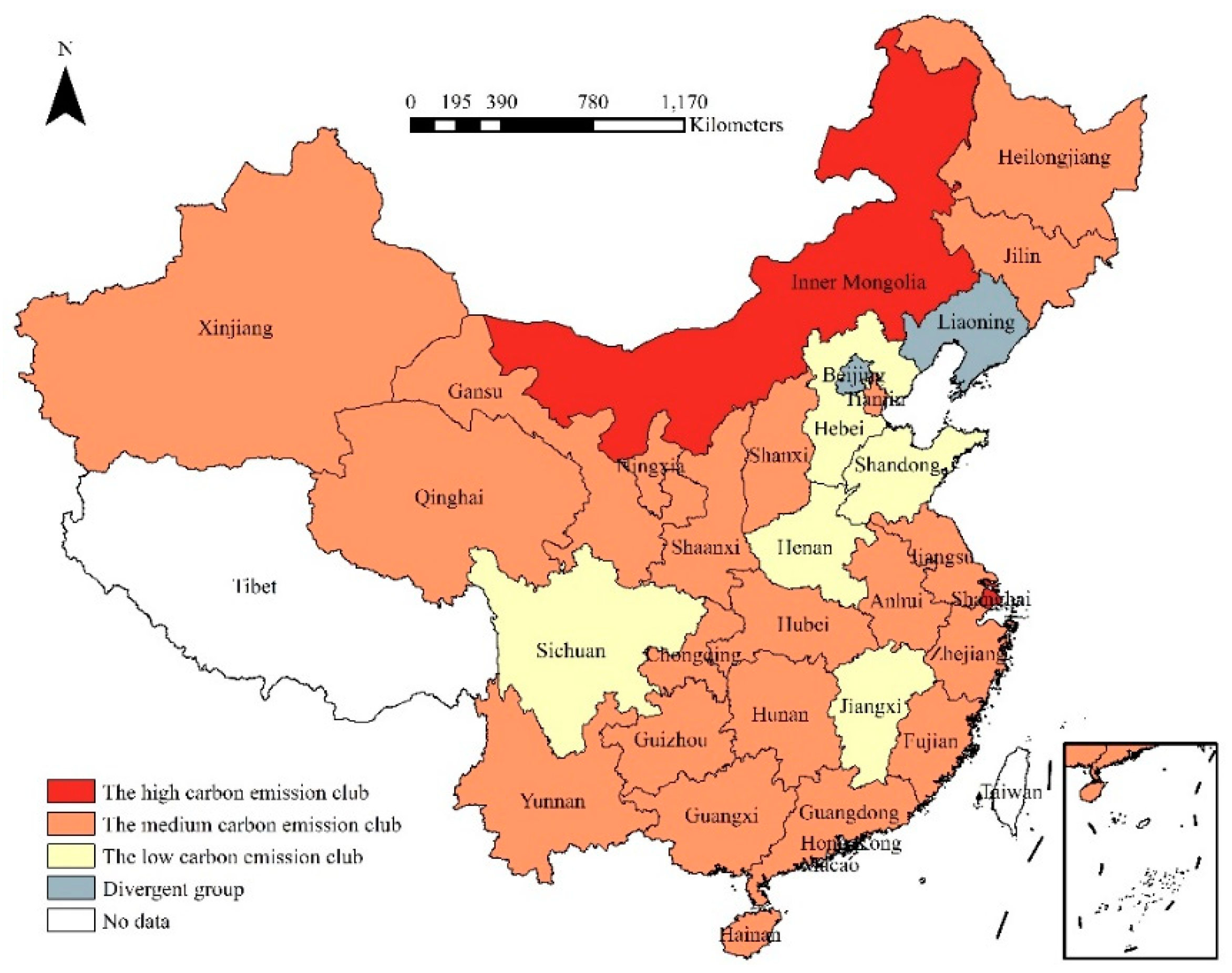
As can be seen from Table 4, the $t$ statistics of the club merging tests on the initial clubs 1 and 2, as well as the initial clubs 2 and 3 are both smaller than −1.65, indicating that these initial clubs fail to pass the merging test. However, the $t$ statistic of the clubs 3 and 4 is 0.2735, which means that they could be merged into the new club 3. Therefore, through the merging test, China’s 30 provinces and municipalities are classified into three convergence clubs and one divergent group, which is shown in

Table 5. Final classification and the main characteristics of various clubs.

Club	Main Characteristics	Membership
Club 1 [2]	With a high level of carbon emissions	Inner Mongolia, Shanghai.
Club 2 [21]	With a medium level of carbon emissions	Tianjin, Shanxi, Jilin, Heilongjiang, Jiangsu, Zhejiang, Anhui, Fujian, Hubei, Hunan, Guangdong, Guangxi, Hainan, Chongqing, Guizhou, Yunnan, Shaanxi, Gansu, Qinghai, Ningxia, Xinjiang.
Club 3 [5]	With a low level of carbon emissions	Hebei, Jiangxi, Shandong, Henan, Sichuan.
Divergent group [2]		Beijing, Liaoning

Notes: the values in the square brackets are the number of club members.

. For the three convergence clubs, their mean values of per capita transportation carbon emissions significantly varied. As can be seen from

Table 6. Descriptive statistics of the convergence clubs.

Club	Sample Size	Mean Value	Standard Deviation	Max.	Min.
Club 1 [2]	22	0.3622	0.1215	0.5014	0.1462
Club 2 [21]	231	0.1098	0.0390	0.2199	0.0268
Club 3 [5]	55	0.0716	0.0334	0.1775	0.0316

, Club 1, only consisting of 2 members, has the highest mean value of 0.3662; Club 2, consisting of 21 members, has the medium mean value of 0.1098; Club 3, consisting of 5 members, has the lowest mean value of 0.0716. Therefore, the convergence clubs 1, 2, and 3 are defined as the high carbon emission club, the medium carbon emission club, and the low carbon emission club, respectively. The spatial distribution of the three convergence clubs and one divergent group is shown in Figure 1.

As can be seen from Table 5, the high carbon emission club only consists of Inner Mongolia and Shanghai. The main reasons are as follows: (1) as the center of the economy in China, Shanghai is not only an important land transportation hub in eastern China, but also closely linked to the central and western provinces. Moreover, it is also an important port city connecting China to the world with huge flows of people and goods. According to the calculation results using statistical data, its traffic turnover volume ranks first in China from 2005 to 2015. (2) Inner Mongolia has a vast territory and is adjacent to various provinces. On the one hand, although it has a relatively low economic development level and relatively backward energy-saving and emission reduction technologies, its traffic infrastructure construction is relatively perfect. For instance, its railway operating mileage ranks first and highway mileage ranks ninth in China in 2016 (National Bureau of Statistics of the People’s Republic of China, 2018) [29]. On the other hand, Inner Mongolia has rich mineral resources, thus increasing the freight turnover between it and the other provinces/municipalities. Obviously, its freight turnover volume is at the forefront of China. The above two reasons led to a large amount of transportation carbon emissions. Meanwhile, Inner Mongolia has a relatively small population, ultimately resulting in relatively high per capita transportation carbon emissions.

The medium carbon emission club consisted of 21 members covering the eastern, central and western regions in China. To be specific, the provinces in the western region have a relatively small population and a relatively low demand for transportation. However, its resources are rich in energy and its technology is relatively backward, which requires more energy to transport local resources. In this club, Hunan, Hubei, Anhui, and Shanxi provinces are located in the hinterland of China and easily accessible. Meanwhile, they are the main labor outflow provinces in China, thus resulting in relatively high transportation carbon emissions. Although the eastern coastal provinces, such as Jiangsu, Zhejiang, Guangdong, Tianjin, etc., have relatively advanced energy-saving and emission reduction technologies which can reduce transportation carbon emissions to some extent, they have a relatively developed economy, frequent foreign trade, and population movements. For example, Guangdong and Jiangsu have a relatively developed foreign trade, and attract large population inflows. In 2016, they respectively rank first and second with respect to the total import and export of goods in China. Therefore, the per capita transportation carbon emissions in those eastern coastal provinces converged to the medium carbon emission club.

The low carbon emission club consisted of 5 provinces including Hebei, Jiangxi, Shandong, Henan, and Sichuan with a large population. Among the top six provinces in population of China, four provinces are included in this club. Despite that they have a large amount of transportation carbon emissions due to the limitation of economy and technological development, they are affected by the average effect of the huge population, eventually converging to low-carbon clubs.

Different from the previous studies (Wang et al., 2014; Hao et al., 2015) [14,16], the classification of convergence clubs in this article does not overlap with the geographical division of China, which fully demonstrates that the log t regression test method and the club clustering algorithm could identify the common characteristics of different regions. The geographical location is not the primary factor for the formation of convergence clubs in China.

4. Analysis of the Factors Influencing the Convergence

In order to further explore the reasons for the formation of the convergence clubs, we will analyze the factors influencing the club convergence of per capita transportation carbon emissions.

First, the dependent variable is the convergence club type of per capita transportation carbon emissions in China. According to the above results, the high carbon emission club, the medium carbon emission club, and the low carbon emission club are assigned the values of 1, 2, and 3, respectively. The higher the value, the better the performance of per capita transportation carbon emissions.

Second, we consider the following independent variables: (1) the development level of the transportation sector which is measured by the per capita transportation output; (2) the intensity of environmental regulation, measured by the proportion of industrial pollution control investment completion to local GDP; (3) the energy intensity of the transportation sector is measured by the ratio of regional transportation energy consumption to local GDP; (4) the energy structure of the transportation sector is represented by the consumption ratio of non-clean energy (specifically coke, raw coal, fuel oil, diesel, and crude oil) in energy consumption of the transportation industry; (5) the urbanization level which is measured by the ratio of the local urban population in the total population; (6) the relative price of energy is measured by the ratio of the purchasing price index of fuel and power to the ex-factory price indices of industrial products. The price is deflated to the price level of 2001; (7) and the fixed assets investment intensity of the transportation sector is measured by the per capita fixed assets investment of the transportation sector. In order to avoid the selection of defects such as outliers or statistical errors that may be caused by specific data for a certain year, all independent variables are the average of the 11-year data for 2005–2015. The above data is derived from the China Population and Employment Statistics Yearbook and China Statistical Yearbook, the provincial statistical yearbooks, and the National Bureau of Statistics of the People’s Republic of China.

Because the dependent variable is discrete ordered data, following the Mckelvey and Zavoina (1975) and Liu et al. (2018) [30,31], we use the Ordered Logit model to explore the factors influencing the club convergence of per capita transportation carbon emissions in China, as shown below:

Let $Y_i$ be an ordered dependent variable which is assigned with the values of c (c = 1, 2, 3), and $X_i$ be the vector of the independent variables, where i denotes the province/municipality i. Let $p_{ic}$ be the probability that the individual i is assigned with the dependent variable c. Then, the cumulative probability distribution function can be defined as:

$$F_{ic}=\mathrm{Pr}\left(Y_i\le y_c{X}_i\right)$$

(9)

Based on the cumulative probability of the ordered dependent variable, the Ordered Logit model establishes the relationship between the independent variables and the club type probability sets:

$$\log \left(\frac{F_{ic}}{1-F_{ic}}\right)=\beta X_i+{\epsilon }_c$$

(10)

where, $\beta X_i={\beta }_1{x}_{i1}+{\beta }_2{x}_{i2}+\dots +{\beta }_7{x}_{i7}$. Specifically, $\beta$ is the estimate of coefficient. And the results are shown in

Table 7. Regression results of the factors influencing the club convergence.

Variables	Regression Coefficients	Marginal Effects
		High Carbon Emission Club	Medium Emission Carbon club	Low Carbon Emission Club
Development level of the transportation sector	1.8238 (1.02)	−0.0397 (−0.77)	−0.0611 (−0.94)	0.1008 (0.89)
Intensity of environmental regulation	4.9313 (1.64)	−0.1074 (−1.28)	−0.1651 (−1.50)	0.2725 (1.56)
Energy intensity of the transportation sector	−118.17 *** (−3.25)	2.5727 *** (2.70)	3.9565 *** (2.91)	−6.5292 *** (−6.30)
Energy structure of the transportation sector	−4.7842 (−0.70)	0.1042 (0.59)	0.1602 (0.79)	−0.2643 (−0.71)
Urbanization level	−32.858 ** (−2.51)	0.7153 ** (2.19)	1.1001 ** (1.97)	−1.8156 *** (−2.69)
Relative price of energy	18.0615 (0.33)	−0.3932 (−0.36)	−0.6047 (−0.32)	0.9980 (0.33)
Fixed assets investment intensity of the transportation sector	−26.698 ** (−2.02)	0.5813 ** (2.46)	0.8939 (1.58)	−1.4752 ** (−2.19)
N	28		LR Chi2	17.05
Prob (LR statistic)	0.0170		Log likelihood	−6.9595
Pseudo R2	0.6509

Notes: ***, **, and * represent the significant levels at 1%, 5%, and 10%, respectively; the values in the parentheses are the z statistic of the corresponding coefficient.

. The table also reports the regression coefficient and the marginal effects of independent variables.

As can be seen from Table 7, the coefficient of the energy intensity of the transportation sector is significantly negative at the 1% confidence level, which shows that provinces with higher energy intensity of transportation will be more inclined to converge into high carbon emission clubs. The reason is that the energy intensity of transportation reflects the energy efficiency of the transportation industry in a region. The increase in energy consumption directly leads to an increase in carbon emissions, which results in the province tending to converge into clubs with high carbon emission levels.

The coefficient of the urbanization level is significantly negative at the 5% level. The provinces with higher urbanization levels tend to converge into clubs with high carbon emission levels, which is consistent with the findings of most of the existing literature (Wu et al., 2016; Li et al., 2017) [7,32]. On the one hand, the increase in urban population has increased demand for transportation in the region; on the other hand, with the improvement of the urbanization level, more economic exchange activities will be generated within regions and sufficient transportation capacity is needed to support the economic development of the city, which will eventually lead to the gradual convergence of the region into clubs with high carbon emission levels.

The coefficient of the fixed assets investment intensity of the transportation sector is significantly negative at the 5% confidence level, it is more likely that provinces with higher investment in fixed assets of transportation will converge to clubs with high carbon emission levels. The main reason is that the expansion of fixed assets investment of the transportation will promote the expansion of the transportation industry, which will consume more energy and generate a large amount of carbon emissions.

Finally, the coefficients of the development level and the energy structure of the transportation sector, as well as the relative price of energy are not significant; these variables do not affect the club convergence (see Supplementary Materials).

5. Conclusions and Policy Implication

The CO₂ emissions from the transportation sector accounts for nearly a quarter of the total CO₂ emissions (International Energy Agency, 2017) [9]. Since 1985, the average annual growth rate of the energy consumption in the transportation sector has been close to 8% in China, which is much higher than the average annual growth rate of the total energy consumption of 5.7% (Yuan et al., 2017), thereby driving the rapid growth of the transportation carbon emissions with an average annual growth rate of 10.56% (Wang et al., 2011) [10,33]. Therefore, studying the convergence of the transportation carbon emissions in China and its influencing factors is of great significance for the reduction of carbon emissions both in China and the world.

This article adopts the log t regression test method and the club clustering algorithm proposed by Phillips and Sul (2007) to explore the convergence characteristics of per capita transportation carbon emissions in China’s provinces and municipalities [12,13,14,15]. Compared with the existing researches on club convergence of carbon emissions in China, this article not only identifies the characteristics of the club convergence of per capita transportation carbon emissions in China in a better manner, but also explores the factors influencing club convergence. Unfortunately, although this article has carried out a certain degree of improvement and innovation in research methods and research content, there are still some shortcomings. For example, due to the inability to obtain statistics on carbon emissions from transportation at the municipal level in China, when studying the factors affecting the convergence of China’s per capita transportation carbon emission clubs, there are only 28 provinces in the Ordered Logit regression model, and the sample size is too small. Moreover, the study period is relatively short. If there are official or authoritative organizations in the future to publish more comprehensive statistics on prefecture-level cities, we will conduct further in-depth research.

Based on the above conclusions, this article proposes the following policy suggestions on the reduction of the transportation carbon emissions in China:

First, the per capita transportation carbon emissions in China converged to three clubs with different carbon emission levels. Therefore, in order to reduce the transportation carbon emissions in China, Chinese governments should develop different emission reduction policies for different clubs. Specifically, for the high carbon emission club with only two members, rigorous environmental laws and regulations, as well as other related measures can be implemented, and the investment in environmental protection and governance should be increased; for the medium carbon emission club with many members, most of them have a relatively low economic development level and a relatively low science and technology level. Therefore, the government should strive to develop science and technology to promote the reduction of carbon emissions from the transportation sector and other sectors. The specific measures are as follows: (1) provide transportation enterprises with corresponding subsidies to purchase environmental protection equipment; (2) strengthen the cultivation of high-tech talents; (3) increase the investment in research and development of energy-saving and environmental protection technologies; (4) establish and perfect relevant institutions to promote the transformation and utilization of energy-saving and emission reduction technologies; for the low carbon emission club, its members have a large population. So, relevant policies should be formulated to improve public transportation facilities and control the number of private cars.

Second, there is a large gap between economic and technological development between clubs and members of the club. Therefore, it is necessary to improve the relevant institutions to promote clean energy and energy-saving technologies, as well as the flow of talents, and strengthen exchanges and cooperation between various clubs and members of the club in terms of transportation carbon emission reduction.

Finally, from the results of the Ordered Logit regression, we can know that the transportation department would adopt advanced energy-saving and emission reduction technologies to improve energy efficiency. At the same time, we must also innovate transportation tools, develop and promote new energy vehicles, and eliminate high-emission transportation vehicles. In terms of investment in transportation, the government cannot blindly expand the scale of transportation through investment, strive to improve transportation carrying capacity on the basis of the original scale through scientific management and planning. In addition, it is necessary to appropriately control the scale of the city, improve and rationally plan the various functional areas of the city, and promote the green and healthy development of the city.

References

- Yu, S.W.; Hu, X.; Fan, J.L.; Cheng, J.H. Convergence of carbon emissions intensity across Chinese industrial sectors. J. Clean. Prod. 2018, 194, 179–192. [Google Scholar] [CrossRef]
- Stegman, A.; Mckibbin, W.J. Convergence and Per Capita Carbon Emission; Brookings Discussion Papers; The Brookings Institution: Washington, D.C., USA, 2005; pp. 171–175. [Google Scholar]
- Hu, Z.Y.; Tang, L.W.; Su, J. Convergence of provincial carbon emission intensity and dynamic processes. Resour. Sci. 2015, 37, 142–151. (In Chinese) [Google Scholar]
- Zhao, X.T.; Burnett, J.W.; Lacombe, D.J. Province-level convergence of China’s carbon dioxide emissions. Appl. Energy 2015, 150, 286–295. [Google Scholar] [CrossRef]
- Huang, B.; Meng, L.N. Convergence of per capita carbon dioxide emissions in urban China: A spatio-temporal perspective. Appl. Geogr. 2013, 40, 21–29. [Google Scholar] [CrossRef]
- Wang, J.; Zhang, K.Z. Convergence of carbon dioxide emissions in different sectors in China. Energy 2014, 65, 605–611. [Google Scholar] [CrossRef]
- Li, J.B.; Huang, X.J.; Yang, H.; Chuai, X.W.; Wu, C.Y. Convergence of carbon intensity in the Yangtze River Delta, China. Habitat Int. 2017, 60, 58–68. [Google Scholar] [CrossRef]
- Lin, B.Q.; Xie, C.P. Reduction potential of CO2 emissions in China’s transport industry. Renew. Sustain. Energy Rev. 2014, 33, 689–700. [Google Scholar] [CrossRef]
- International Energy Agency (IEA). CO2 Emissions from Fuel Combustion Highlights 2017 [EB/OL]. Available online: http://www.iea.org/publications/freepublications/publication/co2-emissions-from-fuel-combustion-highlights-2017.html (accessed on 17 December 2017).
- Wang, W.W.; Zhang, M.; Zhou, M. Using LMDI method to analyze transport sector CO2 emissions in China. Energy 2011, 36, 5909–5915. [Google Scholar] [CrossRef]
- Herrerias, M.J. The environmental convergence hypothesis: Carbon dioxide emissions according to the source of energy. Energy Policy 2013, 61, 1140–1150. [Google Scholar] [CrossRef]
- Yao, S.J.; Zhang, Z.Y. On regional inequality and diverging clubs: A case study of contemporary China. J. Comp. Econ. 2001, 29, 466–484. [Google Scholar] [CrossRef]
- Zhang, Z.Y.; Liu, A.Y.; Yao, S.J. Convergence of China’s regional incomes: 1952–1997. China Econ. Rev. 2001, 12, 243–258. [Google Scholar] [CrossRef]
- Hao, Y.; Zhang, Q.X.; Zhong, M.; Li, B.H. Is there convergence in per capita SO2 emissions in China? An empirical study using city-level panel data. J. Clean. Prod. 2015, 108, 944–954. [Google Scholar] [CrossRef]
- Phillips, P.C.B.; Sul, D. Transition Modeling and Econometric Convergence Tests. Econometrica 2007, 75, 1771–1855. [Google Scholar] [CrossRef] [Green Version]
- Wang, Y.M.; Zhang, P.; Huang, D.K.; Cai, C.D. Convergence behavior of carbon dioxide emissions in China. Econ. Model. 2014, 43, 75–80. [Google Scholar] [CrossRef]
- Apergis, N.; Payne, J.E. Per capita carbon dioxide emissions across U.S. states by sector and fossil fuel source: Evidence from club convergence tests. Energy Econ. 2017, 63, 365–372. [Google Scholar] [CrossRef]
- Ghosh, M.; Ghoshray, A.; Malki, I. Regional divergence and club convergence in India. Econ. Model. 2013, 30, 733–742. [Google Scholar] [CrossRef]
- Tian, X.; Zhang, X.H.; Zhou, Y.H.; Yu, X.H. Regional income inequality in China revisited: A perspective from club convergence. Econ. Model. 2016, 56, 50–58. [Google Scholar] [CrossRef]
- Parker, S.; Liddle, B. Economy-wide and manufacturing energy productivity transition paths and club convergence for OECD and non-OECD countries. Energy Econ. 2016, 62, 338–346. [Google Scholar] [CrossRef]
- Apergis, N.; Christou, C.; Miller, S.M. Country and industry convergence of equity markets: International evidence from club convergence and clustering. N. Am. J. Econ. Financ. 2014, 29, 36–58. [Google Scholar] [CrossRef]
- Xiao, F.; Hu, Z.H.; Wang, K.X.; Fu, P.H. Spatial Distribution of Energy Consumption and Carbon Emission of Regional Logistics. Sustainability 2015, 7, 9140–9159. [Google Scholar] [CrossRef] [Green Version]
- Burnett, J.W. Club convergence and clustering of U.S. energy-related CO2 emissions. Resour. Energy Econ. 2016, 46, 62–84. [Google Scholar] [CrossRef]
- Ulucak, R.; Apergis, N. Does convergence really matter for the environment? An application based on club convergence and on the ecological footprint concept for the EU countries. Environ. Sci. Policy 2018, 80, 21–27. [Google Scholar] [CrossRef]
- Du, K.R. Econometric convergence test and club clustering using Stata. Stata J. 2017, 17, 882–900. [Google Scholar] [CrossRef]
- Schnurbus, J.; Haupt, H.; Meier, V. Economic Transition and Growth: A Replication. J. Appl. Econ. 2017, 32, 1039–1042. [Google Scholar] [CrossRef]
- Li, H.Q.; Lu, Y.; Zhang, J.; Wang, T.Y. Trends in road freight transportation carbon dioxide emissions and policies in China. Energy Policy 2013, 57, 99–106. [Google Scholar] [CrossRef]
- Wang, Y.P.; Yan, W.L.; Ma, D.; Zhang, C.L. Carbon emissions and optimal scale of China’s manufacturing agglomeration under heterogeneous environmental regulation. J. Clean. Prod. 2018, 176, 140–150. [Google Scholar] [CrossRef]
- NBSC (National Bureau of Statistics of the People’s Republic of China). China Statistical Yearbook 2017; China Statistics Press: Beijing, China, 2018. (In Chinese)
- Mckelvey, R.D.; Zavoina, W. A Statistical Model for the Analysis of Ordinal Level Dependent Variables. J. Math. Sociol. 1975, 4, 103–120. [Google Scholar] [CrossRef]
- Liu, C.; Hong, T.; Li, H.F.; Wang, L.L. From club convergence of per capita industrial pollutant emissions to industrial transfer effects: An empirical study across 285 cities in China. Energy Policy 2018, 121, 300–313. [Google Scholar] [CrossRef]
- Wu, Y.Z.; Shen, J.H.; Zhang, X.L.; Skitmore, M.; Lu, W.S. The impact of urbanization on carbon emissions in developing countries: A Chinese study based on the U-Kaya method. J. Clean. Prod. 2016, 135, 589–603. [Google Scholar] [CrossRef]
- Yuan, C.W.; Zhang, S.; Jiao, P.; Wu, D.Y. Temporal and spatial variation and influencing factors research on total factor efficiency for transportation carbon emissions in China. Resour. Sci. 2017, 39, 687–697. (In Chinese) [Google Scholar]
Figure 1.
The spatial distribution of convergence clubs and divergent group.