Multi-Objective Cloud Manufacturing Service Selection and Scheduling with Different Objective Priorities

Abstract

In recent years, with the support of new information technology and national policies, cloud manufacturing (CMfg) has developed rapidly in China. About CMfg, scholars have conducted extensive and in-depth research, among which multi-objective service selection and scheduling (SSS) attracts increasing attention. Generally, the objectives of the SSS problem involve several aspects, such as time, cost, environment and quality. In order to select an optimal solution, the preference of a decision maker (DM) becomes key information. As one kind of typical preference information, objective priorities are less considered in current studies. So, in this paper, a multi-objective model is first constructed for the SSS with different objective priorities. Then, a two-phase method based on the order of priority satisfaction (TP-OPS) is designed to solve this problem. Finally, computational experiments are conducted for problems with different services and tasks/subtasks, as well as different preference information. The results show that the proposed TP-OPS method can achieve a balance between the maximum comprehensive satisfaction and satisfaction differences, which is conducive to the sustainable development of CMfg. In addition, the proposed method allows the preference information to be gradually clarified, which has the advantage of providing convenience to DM.

1. Introduction

In recent years, information technologies have been widely used in manufacturing companies, and their impacts on the manufacturing industry become more apparent than ever before [1,2,3]. In order to promote manufacturing informationization, major manufacturing countries in the world have issued relevant policies, which provide an unprecedented opportunity for the sustainable development of the manufacturing industry. As a new manufacturing model supported by information technology, cloud manufacturing (CMfg) is rapidly developing in China [4,5]. Through CMfg platforms, manufacturing resources distributed throughout this country are integrated and packaged into various services. At the same time, a variety of manufacturing requirements are published onto the platforms by clients. These requirements are usually personalized products that need multiple services to work together [6]. Therefore, how to select and schedule these services to meet the requirements of different clients becomes an important issue.

At present, scholars have built various characteristic models for CMfg service selection and scheduling (SSS) problems [7] (or service composition [8], task scheduling [9,10] and service sharing [11,12]). Tao et.al. have done a detailed overview on the CMfg service management [13]. One common feature of these models is that multiple factors need to be considered in the objectives, for example, time [14,15,16], cost [14,15,16,17], reliability [14,15,16] and energy consumption [14,17,18,19], risk [17], service [20], trust [21], availability [22], value [23], reputation [19,24] and workload [25]. Some scholars integrate these factors into a single objective through weight values and design effective algorithms, such as the: parallel method [8], workload-based method [9], two-level method [10], cooperative method [26], chaos control optimal algorithm [16] and improved niche immune algorithm [27]. Some focus on the game theory models [11,12]. Some others pay attention to multi-objective models and algorithms; for instance, Pareto group leader algorithm [14], cloud-entropy enhanced genetic algorithm [23], hybrid artificial bee colony algorithm [18,19], adaptive multi-population differential artificial bee colony algorithm [24], modified particle swarm optimization algorithm [25] and ε-dominance multi-objective evolutionary algorithm [28].

In the above studies, novel objective functions attract more attention, and DM’s preference for different objectives is rarely considered or simply expressed as a set of weight values [8,17]. In the decision-making process, preference information is critical due to the fact that only one solution needs to be selected as the final scheme. Therefore, considering preference information in the model or algorithm becomes a new research direction, which can provide convenience for DM to choose satisfactory solutions. So, in our previous paper [29], linguistic preference is taken into account, and a two-phase method based on a desirable satisfying degree is proposed. However, in the real environment, preference information will not always be given in terms of linguistic terms; sometimes, it may be expressed as objective priorities, i.e., the order in which only after some objectives have been achieved, other can be considered. To solve multi-objective optimization problems with priorities, lexicographic optimization is widely used [30,31]. This method divides objectives into $L$ priority levels, where $L$ does not exceed the number of objectives. However, when there are multiple priorities, lexicographic optimization will consume a lot of computation time. Therefore, Chen and Tsai [32] put forward a principle that objectives with high priority have high satisfactions. Based on their ideas, Li and Hu [33] proposed a two-step interactive satisfactory method that decomposed the multi-objective problem into two sub-problems. However, this method is mainly used for continuous optimization problems and not suitable for direct use in discrete optimization. Therefore, this paper plans to improve their method and introduce it into SSS problems.

In this paper, we intend to study an SSS problem with different objective priorities. In particular, the following questions will be answered: (1) How to build an SSS model that takes into account different objective priorities. (2) How to control the satisfaction difference while optimizing all objectives. (3) In the decision-making process, how does DM gradually give clear preference information?

The rest of this paper is structured as follows. Section 2 gives a brief description of the problem. In Section 3, the proposed SSS model and solution method are introduced and analyzed in detail. In Section 4, computational experiments are conducted for problems with different scales and different preference information. Section 5 draws conclusions and gives directions for further research.

2. Problem Description

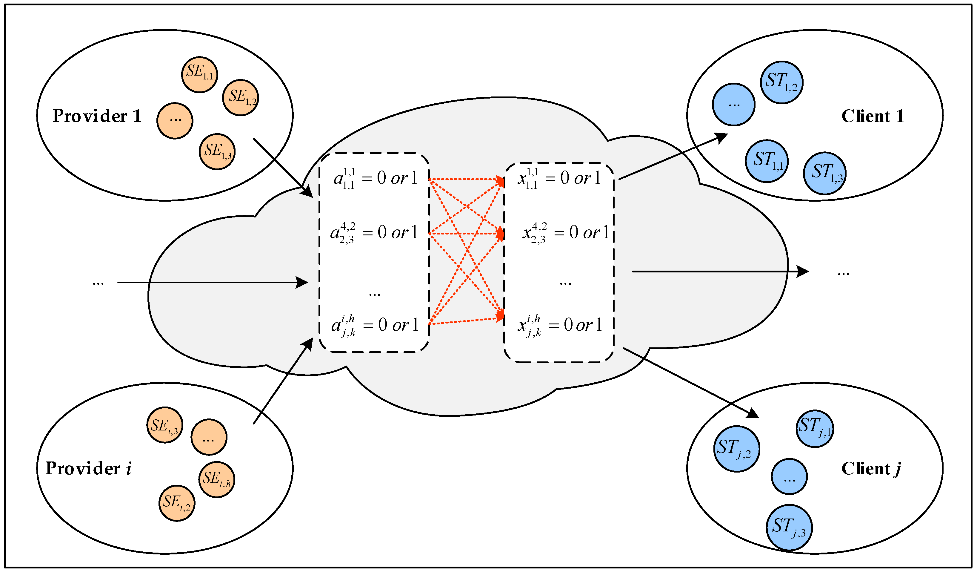
In this research, the CMfg platform with client-centered operating mode is taken into account, where clients’ interests become the optimization objectives. When a client’s request is submitted to the CMfg platform, it usually needs to be allocated to different service providers through three steps: task decomposition, service discovery and matching, service selection and scheduling (SSS). The abstract model of SSS in CMfg is shown in Figure 1 [14]. Suppose that within a certain decision period, there are $M$ enterprises and $N$ tasks on the CMfg platform. Here, we use $E=\left\{E_1,\cdots ,E_i,\cdots ,E_M\right\}$ to represent the enterprise set, and $T=\left\{T_1,\cdots ,T_j,\cdots ,T_N\right\}$ to represent the task set. Different enterprises provide different kinds of services, for example, enterprise $E_i$ provides $H_i$ kinds of services, so it’s service set is expressed as $S{E}_i=\left\{S{E}_{i,1},\cdots ,S{E}_{i,h},\cdots ,S{E}_{i,H_i}\right\}$. Each task could be decomposed into multiple subtasks, for example, task $T_j$ could be decomposed into $K_j$ subtasks, so it’s subtask set is expressed as $S{T}_j=\left\{S{T}_{j,1},\cdots ,S{T}_{j,k},\cdots ,S{T}_{j,K_j}\right\}$. In the SSS process, each subtask is assigned to one available service by $a_{j,k}^{i,h}$ and $x_{j,k}^{i,h}$, both of which can only be 0 or 1. Firstly, the value of $a_{j,k}^{i,h}$ is determined in service discovery and matching process, then treated as a known parameter in SSS process. If service $S{E}_{i,h}$ has the ability to perform subtask $S{T}_{j,k}$, then $a_{j,k}^{i,h}=1$; otherwise $a_{j,k}^{i,h}=0$. Secondly, we need to select the value of $x_{j,k}^{i,h}$ in SSS process. If subtask $S{T}_{j,k}$ is indeed assigned to service $S{E}_{i,h}$, then $x_{j,k}^{i,h}=1$; otherwise $x_{j,k}^{i,h}=0$. For instance in Figure 1, $a_{2,3}^{4,2}$ is used to determine whether service $S{E}_{4,2}$ is capable of executing subtask $S{T}_{2,3}$, and $x_{2,3}^{4,2}$ is used to determine whether subtask $S{T}_{2,3}$ is allocated to service $S{E}_{4,2}$.

Different values of $x_{j,k}^{i,h}$ represent different SSS schemes. As two important factors affecting the results of SSS, DM’s preferences and platform’s operational mode are considered in our studies. Based on these two factors, we classify the SSS problem into different types, as shown in

Table 1. Classification of SSS Problem Based on Preference Information and Operation Mode.

	Mode	Client Centered	Provider Centered	Operator Centered	System Centered
Preference
Linguistic terms					Previouse work
Objective priorities		This paper
Others			Future work	Future work

. For each kind of preference information, we intend to consider a different operation mode. In previous work, we considered linguistic terms and system-centered mode. While in this paper, different objective priorities and client-centered mode are taken into account.

When DM believes that the objective has priority, it is not appropriate to find the Pareto solution set, because it will cost a lot. So, scholars try different methods to get an optimal solution with objective priorities. For example: Khorram and Nozari [34] considered a problem with 3 objectives, each objective function has different priority. We use $f_g$ to reperesent the $g$th objective function, then $f_1$ has the first priority and $f_2$ has the second priority. The priority relationship in their exaple could be expressed as:

Priority level 1: $f_1$;

Priority level 2: $f_2$;

Priority level 3:$f_3$.

In the SSS problem, there are also some situations where some objectives are more important than others. For example, for industries with serious environmental impacts, environmental objectives are more important than cost and time objectives; for urgent tasks, time objectives are more important than cost objectives. Priority is a common type of DM’s preference. According to the objective priorities, an optimal service selection and scheduling scheme can be obtained. For the convenience of modeling, the number of priority level is expressed by the parameter $L$. Here, we consider a three-level priority, i.e., $L=3$. Then, the key becomes how to choose the most preferred solution, which optimizes multiple objectives in collaboration, while reflecting the relative importance based on priority.

3. The Multi-Objective Service Selection and Scheduling Model and Solution Methods

Based on the problem description described in the previous section, the proposed multi-objective SSS model and optimization method are presented in the following subsections.

3.1. Model Formulation

Before modeling, some important notations are shown in

Table 2. A list of some important notations.

Notation	Meaning
$t_j$	Completion time of task $T_j$.
$c_j$	Service cost of task $T_j$.
$q_j$	Service quality of task $T_j$.
$e{c}_j$	Environmental cost of task $T_j$. (client $j$).
$s{t}_{j,k}^{i,h}$	Service time of subtask $S{T}_{j,k}$, if it is assigned to service $S{E}_{i,h}$.
$s{c}_{j,k}^{i,h}$	Service cost of subtask $S{T}_{j,k}$, if it is assigned to service $S{E}_{i,h}$.
$q_{j,k}^{i,h}$	Service quality of subtask $S{T}_{j,k}$, if it is assigned to service $S{E}_{i,h}$.
$e{c}_{j,k}^{i,h}$	Environmental cost of subtask $S{T}_{j,k}$, if it is assigned to service $S{E}_{i,h}$.
$w{e}_{j,k}^{i,h}$	Weight of products needed to be transported, if subtask $S{T}_{j,k}$ is assigned to service $S{E}_{i,h}$.
$a{t}_{j,k}$	Start time of subtask $S{T}_{j,k}$.
$c{t}_{j,k}$	Completion time of subtask $S{T}_{j,k}$.
$w{t}_{j,k}$	Waiting time of subtask $S{T}_{j,k}$.
$l{t}_{j,k}$	Logistics time from subtask $S{T}_{j,k}$ to $S{T}_{j,k+1}$.
$l{c}_{j,k}$	Logistics cost from subtask $S{T}_{j,k}$ to $S{T}_{j,k+1}$.
$d_{i,i^{\prime }}$	Geographical distance between enterprises $E_i$ and $E_i$.
$\alpha$	Logistics time for unit distance.
$\beta$	Logistics cost for unit weight and unit distance.
$a_{j,k}^{i,h}$	$a_{j,k}^{i,h}=1$, if service $S{E}_{i,h}$ can perform subtask $S{T}_{j,k}$; otherwise $a_{j,k}^{i,h}=0$.
$x_{j,k}^{i,h}$	$x_{j,k}^{i,h}=1$, if subtask $S{T}_{j,k}$ is assigned to service $S{E}_{i,h}$; otherwise $x_{j,k}^{i,h}=0$.

.

In SSS problems, some basic constraints need to be subjected to. First of all, this paper considers the case where a subtask can only be assigned to one service. Then, the constraint can be expressed as:

$${\sum }_{i=1}^M{\sum }_{h=1}^{H_i}{x}_{j,k}^{i,h}=1,\forall j=1,\cdots ,N;k=1,\cdots ,K_j$$

(1)

Second, task $S{T}_{j,k}$ can be assigned to service $S{E}_{i,h}$, only if service $S{E}_{i,h}$ is able to perform subtask $S{T}_{j,k}$. This constraint can avoid illogical arrangements, and be expressed as:

$$x_{j,k}^{i,h}\le a_{j,k}^{i,h},\forall j=1,\cdots ,N;k=1,\cdots ,K_j$$

(2)

In addition, $x_{j,k}^{i,h}$ is a logical variable, and could only be 0 or 1.

$$x_{j,k}^{i,h}\in \left\{0,1\right\},\forall j=1,\cdots ,N;i=1,\cdots ,M;k=1,\cdots ,K_j;h=1,\cdots ,H_i$$

(3)

Different from previous studies, our objective functions are client-centered. In this mode, it is suitable to use the pay-per-use method to meet the needs of clients and improve their satisfaction. In order to promote the sustainability of CMfg, the average satisfaction of clients with the time, cost quality and environmental cost of their tasks are considered in this paper, expressed as $U_t$, $U_c$, $U_q$, $U_{ec}$. Therefore, multiple objectives are as follows:

$$f_1=U_t=\left({\sum }_{j=1}^N{\mu }_j^t\right)/N$$

(4)

$$f_2=U_c=\left({\sum }_{j=1}^N{\mu }_j^c\right)/N$$

(5)

$$f_3=U_q=\left({\sum }_{j=1}^N{\mu }_j^q\right)/N$$

(6)

$$f_4=U_{ec}=\left({\sum }_{j=1}^N{\mu }_j^{ec}\right)/N$$

(7)

where, ${\mu }_j^t$, ${\mu }_j^c$, ${\mu }_j^q$, ${\mu }_j^{ec}$ are respectively the satisfaction of the client (task) $j$.

Satisfaction of the clients are all calculated based on the limits given by clients, shown as:

$${\mu }_j^t=\{\begin{array}{ll}1\hfill & t_j\ge t_j^{max}\hfill \\ \left(t_j-t_j^{min}\right)/\left(t_j^{max}-t_j^{min}\right)\hfill & t_j^{min}\le t_j<t_j^{max}\hfill \\ 0\hfill & t_j<t_j^{min}\hfill \end{array}$$

(8)

$${\mu }_j^c=\{\begin{array}{ll}1\hfill & c_j\ge c_j^{max}\hfill \\ \left(c_j-c_j^{min}\right)/\left(c_j^{max}-c_j^{min}\right)\hfill & c_j^{min}\le c_j<c_j^{max}\hfill \\ 0\hfill & c_j<c_j^{min}\hfill \end{array}$$

(9)

$${\mu }_j^q=\{\begin{array}{ll}1\hfill & q_j\ge q_j^{min}\hfill \\ 1-\left(q_j-q_j^{min}\right)/\left(q_j^{max}-q_j^{min}\right)\hfill & q_j^{min}\le q_j<q_j^{max}\hfill \\ 0\hfill & q_j<q_j^{max}\hfill \end{array}$$

(10)

$${\mu }_j^{ec}=\{\begin{array}{ll}1\hfill & e{c}_j\ge e{c}_j^{max}\hfill \\ \left(e{c}_j-e{c}_j^{min}\right)/\left(e{c}_j^{max}-e{c}_j^{min}\right)\hfill & e{c}_j^{min}\le e{c}_j<e{c}_j^{max}\hfill \\ 0\hfill & e{c}_j<e{c}_j^{min}\hfill \end{array}$$

(11)

where $t_j^{max}$, $t_j^{min}$, $c_j^{max}$, $c_j^{min}$, $q_j^{max}$, $q_j^{min}$, $e{c}_j^{max}$, $e{c}_j^{min}$ are the upper and lower limits of time, cost, quality, and environmental cost given by clients. They are the upper and lower limits of time, cost, quality, and environmental cost given by the user. For example, the completion period given by client $j$ is $t_j^{max}$, and the ideal completion time is $t_j^{min}$. Client $j$ is most dissatisfied when the actual completion time $t_j$ exceeds $t_j^{max}$, and most satisfied when $t_j$ is less than $t_j^{max}$. Detailed calculations of $t_j$, $c_j$, $q_j$ and $e{c}_j$, are shown in our previous paper [26].

The above objectives (4)–(7) need to be maximized, and the following equation is introduced to indicate the satisfaction of DM with each objective.

$${\mu }_{f_g}=\{\begin{array}{ll}1\hfill & f_g\ge f_g^{max}\hfill \\ \left(f_g-f_g^{min}\right)/\left(f_g^{max}-f_g^{min}\right)\hfill & f_g^{min}\le f_g<f_g^{max}\hfill \\ 0\hfill & q_j<q_j^{min}\hfill \end{array}$$

(12)

where, $f_g^{min}$ and $f_g^{max}$ are obtained directly by DM or solving each objective.

Then the objective function becomes:

$$\max \left({\mu }_{f_1},{\mu }_{f_2},{\mu }_{f_3},{\mu }_{f_4}\right)$$

(13)

When DM has priority requirements for each objective, the multi-objective optimization problem is expressed as:

$$\max \left[P_1\left(f_1^1,\cdots ,f_{N_1}^1\right),\cdots ,P_l\left(f_1^l,\cdots ,f_{N_l}^l\right),\cdots ,P_L\left(f_1^L,\cdots ,f_{N_L}^L\right)\right]$$

(14)

where $P_l$ represents the set of objectives with priority $l$. In Equation (14), if $P\left(f_g\right)=l$, then $f_g\in P_l$. $P_l$ has higher priority than $P_{l+1}$, for $l=1,\cdots ,L$.

Usually, this kind of problem is solved by lexicographic optimization. However, considering its low computation efficiency, some researchers simplified the original optimization problem. Chen and Tsai [29] proposed that objectives with high priority have high satisfactions. According to their ideas, the priority order could be expressed as:

$${\mu }_{f_g}\ge {\mu }_{f_{g^{\prime }}}, \forall P\left(f_g\right)<P\left(f_{g^{\prime }}\right)$$

(15)

where $P\left(f_g\right)<P\left(f_{g^{\prime }}\right)$ mean that the priority level of the $j$th objective is higher than the j’th.

Then they transformed the objective function (14) into the following problem by FGP method:

$$\{\begin{array}{l}\max TS={\sum }_{g=1}^G{\mu }_{f_g}\hfill \\ {\mu }_{f_g}\ge {\mu }_{f_{g^{\prime }}}, P\left(f_g\right)<P\left(f_{g^{\prime }}\right)\hfill \end{array}$$

(16)

However, Equation (15) narrows the scope of feasible solutions and is not conducive to optimization. Therefore, in order to avoid this situation, $\epsilon$ is introduced to relax the comparison relationship:

$${\mu }_{f_g}-{\mu }_{f_{g^{\prime }}}\ge \epsilon ,\forall P\left(f_g\right)<P\left(f_{g^{\prime }}\right), g,g^{\prime }=1,2,\cdots ,G$$

(17)

only when $\epsilon \ge 0$, the result meets the priority requirement.

In order to make the method more suitable for real decision making, Li and Hu [30] proposed a two-step interactive satisfactory method. We combine it with genetic algorithm and introduce into the SSS problem. GA algorithm is widely used in various types of scheduling problems and has strong applicability. While GA is not necessary, other intelligent algorithms may get better results. On the basis of previous research, we introduce the order of priority satisfaction, and propose a two-phase method based on the order of priority satisfaction (TP-OPS). In phase 1, comprehensive satisfaction $\mathsf{\lambda }$ is maximized.

Phase 1:

$$\{\begin{array}{l}\max \mathsf{\lambda }\hfill \\ s.t. {\mu }_{f_g}\ge \lambda ,g=1,2,\cdots ,G\hfill \\ \begin{array}{l}0\le {\mu }_{f_g}\le 1\hfill \\ \left(1\right)~\left(3\right)\hfill \end{array}\hfill \end{array}$$

(18)

where, the decision variable is $x_{j,k}^{i,h}$. We define the optimal solution ${\lambda }^{*}$ as the maximum comprehensive satisfaction.

Phase 2:

Through Equation (17), the priorities are divided into different levels. At the same time, $\Delta \delta$ is introduced in the following equation.

$${\mu }_{f_g}\ge {\lambda }^{*}·\Delta \delta$$

(19)

where $\Delta \delta \left(0\le \Delta \delta \le 1\right)$ is used to relax ${\lambda }^{*}$, which in turn expands the search space. Then, the model in phase 2 is built as:

$$\{\begin{array}{l}\max \mathsf{\epsilon }\hfill \\ s.t. {\mu }_{f_g}\ge {\lambda }^{*}·\Delta \delta ,g=1,2,\cdots ,G\hfill \\ \begin{array}{l} {\mu }_{f_g}-{\mu }_{f_{g^{\prime }}}\ge \epsilon ,\forall P\left(f_g\right)<P\left(f_{g^{\prime }}\right),g,g^{\prime }=1,2,\cdots ,N\hfill \\ 0\le {\mu }_{f_g}\le 1\hfill \\ \left(1\right)~\left(3\right)\hfill \end{array}\hfill \end{array}$$

(20)

where $x_{j,k}^{i,h}$ and $\epsilon$ are the decision variables. Maximizing $\epsilon$ means to maximize satisfaction differences of different objectives.

To illustrate the principle of TP-OPS approach, a simple two-objective example is constructed as follows.

$$\{\begin{array}{l}\max \left({\mu }_{f_1},{\mu }_{f_2}\right)\hfill \\ \hfill \\ s.t. Ax\le b\hfill \end{array}$$

(21)

Suppose that $f_2$ has a higher priority than $f_1$, expressed as:

Priority level 1: $f_2$

Priority level 2: $f_1$

According to Equation (17), we can get that:

$${\mu }_{f_2}-{\mu }_{f_1}\ge \epsilon$$

(22)

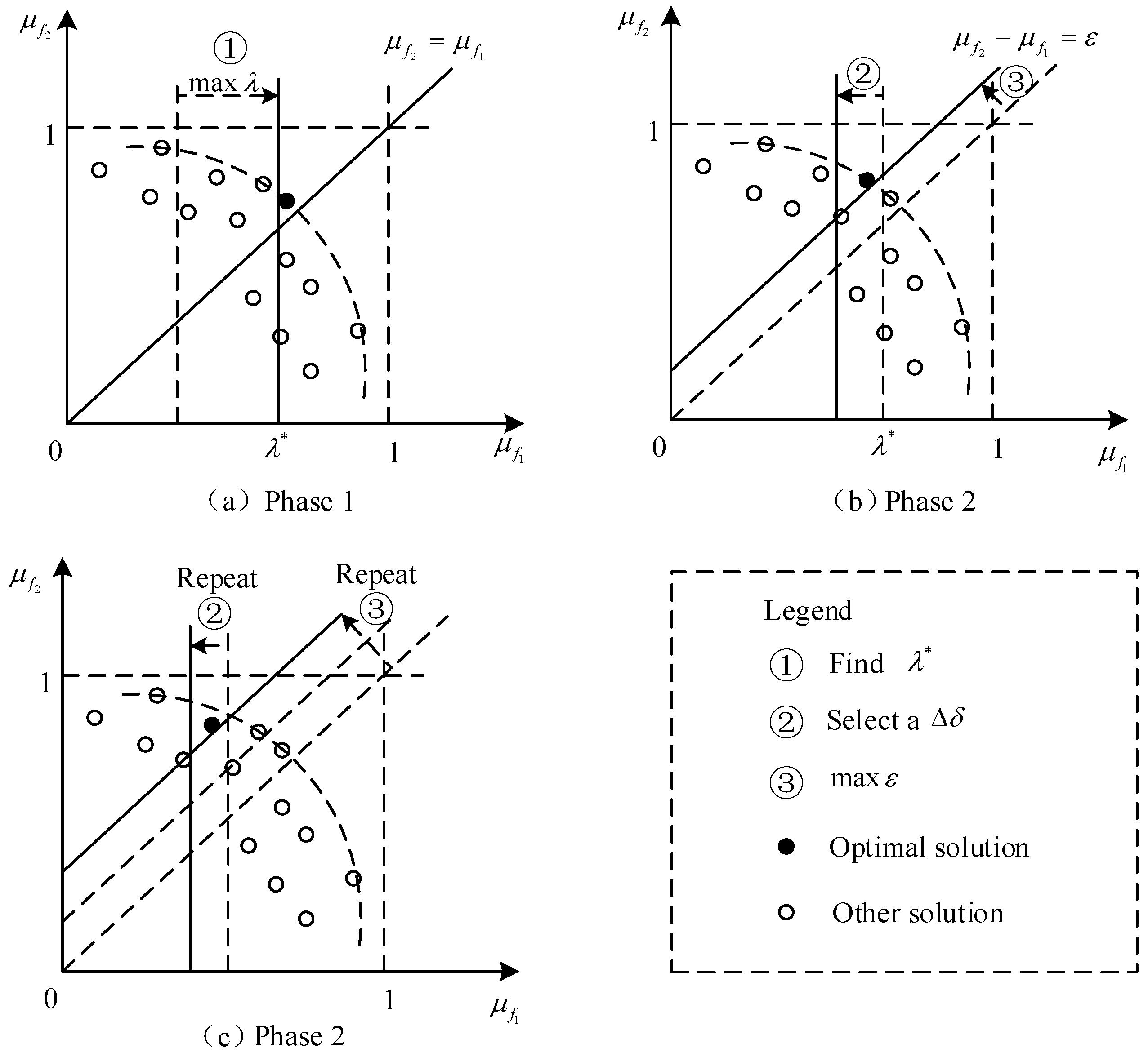
With this example, the priciple of TP-OPS method is shown in Figure 2. As can be seen from Figure 2a, the optimal solution found in phase 1 of maximizing $\mathsf{\lambda }$ is very close to the straight line ${\mu }_{f_1}={\mu }_{f_2}$, that is, the difference of objective satisfaction is very small. If DM is not satisfied with this optimal solution, then set a new $\Delta \delta$ and maximize $\epsilon$, as shown in Figure 2b. The optimal solution found at this time deviates from the straight line ${\mu }_{f_1}={\mu }_{f_2}$ along the Pareto front. If DM still feels that the difference in satisfaction is small, then he could choose a smaller $\Delta \delta$ and look for a larger $\epsilon$. In Figure 2c, the optimal solution is further shifted to the left and further away from the straight line ${\mu }_{f_1}={\mu }_{f_2}$. By repeating ② and ③ in this figure, DM can find a final optimal solution. By objective priorities, TP-OPS does not need to preserve a complete set of Pareto solutions in the calculation process, which is helpful to improve the computational efficiency. If we deal with more objectives, this effect will be more obvious.

3.2. Optimization Method

3.2.1. Different SSS Methods

As mentioned earlier, the tasks that this paper focuses on are all complex tasks. Each complex task must be decomposed into a few simple subtasks that can be executed by existing resource services. The SSS model described in Section 3.1 considers not only DM’s priority preferences, but also the optimization of all tasks from a client-centered perspective. In order to solve the proposed model, we developed the TP-OPS method. In this subsection, the detailed steps will be introduced, while two other methods, the max–min method and the FGP method, will also be introduced for comparison. Figure 3 shows the framework of the three methods.

(1) Max–min method

The max–min method is a conservative method, taking into account the objective of lowest satisfaction. The objective of this method can be expressed by $\max \min \left({\mu }_{f_g}\right)$ or Equation (18). So phase 1 of TP-OPS method is also called Max–min method. However, objective priorities are not considered in this method, which results in that constraint (15) is not necessarily satisfied. We implement this method directly with GA algorithm, and the encoding rules are introduced later.

(2) FGP method

The FGP method is advantageous to consider from the whole point of view, and its objective is expressed in Equation (16). Unlike the Max–min method, this method maximizes the total satisfaction of the objectives, and makes the objective which is easy to improve the satisfaction better satisfied. In addition, DM’s preference is taken into account, and only solutions satisfying priority satisfaction are selected. Similarly, this method is also implemented by GA algorithm, except that only solutions satisfying constraint (15) would be used to compute $TS$ value.

(3) TP-OPS method

The TP-OPS method decomposes the original problem into two sub-problems, corresponding to two phases respectively. The pseudo codes of the TP-OPS method is shown in

Table 3. The pseudo codes of Phase 1.

Phase 1
1.	Initialization:
2.	Set $Na=0$; $S=\varnothing$; $N{a}_{max}$; $K{a}_{max}$; ${\lambda }_0$; $UF=\varnothing$
3.	Generate an initial population;
4.	Iteration:
5.	While$Na<N{a}_{max}$do
6.	$Na\leftarrow Na+1$;
7.	$Ka=0;$
8.	While $Ka<K{a}_{max}$ do
9.	$Ka\leftarrow Ka+1$;
10.	Evaluate ${\mu }_{f_1}^{Ka},\cdots ,{\mu }_{f_4}^{Ka}$ and ${\lambda }^{Ka}$ according to Equation (18);
11.	If ${\lambda }^{Ka}>{\lambda }_0$ and ${\mu }_{f_g}^{Ka}>{\mu }_{f_{g^{\prime }}}^{Ka}$ then
12.	$S\leftarrow S{\cup }^{}\left\{C{h}_{Ka}\right\}$; $UF\leftarrow UF{\cup }^{}\left\{{\mu }_{f_g}^{Ka}\right\}$;
13.	end if
14.	If $\lambda >{\lambda }^{*}$ then
15.	${\lambda }^{*}\leftarrow \lambda$;
16.	end if
17.	end while
18.	Crossover and mutation
19.	end while
20.	Output:
21.	${\lambda }^{*}$, $S$ and $UF$.

and

Table 4. The pseudo codes of Phase 2.

Phase 2
1.	Initialization:
2.	Imput ${\lambda }^{*}$; $S$; $UF$;
3.	Set $Nc=0$; ${\epsilon }_s$; $N{c}_{max}$; $H$; ${\epsilon }^{*}=0$; $\Delta \delta =1$;
4.	Iteration:
5.	While${\epsilon }^{*}<{\epsilon }_s$and$Nc<N{c}_{max}$do
6.	$Nc\leftarrow Nc+1$;
7.	For every $C{h}_{Kc}\subset S$ do
8.	Read ${\mu }_{f_g}^{Kc}$ from $UF$;
9.	If ${\mu }_{f_g}^{Kc}>{\lambda }^{*}\cdot \Delta \delta$ then
10.	Calculate ${\epsilon }^{Kc}$ according to Equation (20);
11.	If ${\epsilon }^{Kc}>{\epsilon }^{*}$ then
12.	${\epsilon }^{*}\leftarrow {\epsilon }^{Kc}$; $C{h}^{*}\leftarrow C{h}_{Kc}$;
13.	end if
14.	end if
15.	end for
16.	If ${\epsilon }^{*}<{\epsilon }_s$ then
17.	$\Delta \delta \leftarrow \Delta \delta -H$;
18.	end if
19.	end while
20.	Output:
21.	${\epsilon }^{*}$ and $C{h}^{*}$.

.

In Phase 1, first, DM chooses a minimum ${\lambda }_0$ as the criterion for saving the feasible solution. Then, Max–min method is performed. In particular, each chromosome that meets ${\lambda }^{Ka}>{\lambda }_0$ and ${\mu }_{f_g}^{Ka}>{\mu }_{f_{g^{\prime }}}^{Ka}$ encountered during the iteration will be stored in the set $S$, and the corresponding satisfaction ${\mu }_{f_g}^{Ka}$ will also be stored in the set $UF$. Every chromosomes in $S$ corresponds to a feasible solution that satisfies constraint (15). If ${\lambda }_0$ is set to a smaller value, then the more chromosomes are saved, the more storage space is occupied. Finally, phase 1 outputs the maximum comprehensive satisfaction ${\lambda }^{*}$, the feasible solution set $S$ and the corresponding satisfaction set $UF$.

In phase 2, first, ${\lambda }^{*}$, $S$ and $UF$ are imputed. In addition, DM chooses the criterion of satisfaction difference ${\epsilon }_s$, and change amount $H$ of $\Delta \delta$ in each iteration. Secondly, all individuals satisfying ${\mu }_{f_g}^{Kc}>{\lambda }^{*}\cdot \Delta \delta$ are selected from $S$ to calculate their ${\epsilon }^{Kc}$. When $\epsilon >{\epsilon }_s$, the difference in satisfaction of different priority targets reaches the set value, and we believe that we have found a satisfactory solution approved by the decision maker. If $\epsilon <{\epsilon }_s$, then $\Delta \delta$ is reduced by $H$, expanding the searched space until a satisfactory solution is found ${\epsilon }^{*}>{\epsilon }_s$ or the maximum number of iterations is reached $Nc>N{c}_{max}$. Finally, Phase 2 outputs the satisfaction difference ${\epsilon }^{*}$ and the corresponding chromosome $C{h}^{*}$.

3.2.2. The GA Algorithm

All three methods are based on a GA algorithm, and multi-layer integer coding rules are adopted to encode chromosomes. When the total number of tasks is N and the number of subtasks of task T_j is $K_j$, the length of individual is $2{\sum }_{j=1}^N{K}_j$. Among them, the first half of the chromosome represents the service order of all tasks in the enterprise, and the second half represents the enterprise services matched by each subtask. For example:

$$\left[\begin{array}{cc}\begin{array}{cc}\begin{array}{cc}\begin{array}{cc}1& 3\end{array}& \begin{array}{cc}3& 4\end{array}\end{array}& \begin{array}{cc}\begin{array}{cc}2& 2\end{array}& \begin{array}{cc}1& 4\end{array}\end{array}\end{array}& \begin{array}{cc}\begin{array}{cc}\begin{array}{cc}2& 3\end{array}& \begin{array}{cc}1& 4\end{array}\end{array}& \begin{array}{cc}\begin{array}{cc}2& 5\end{array}& \begin{array}{cc}6& 3\end{array}\end{array}\end{array}\end{array}\right]$$

(23)

This individual (23) expresses a service order of 4 tasks on 3 enterprises, where each task has 2 subtasks and each enterprise has 2 services. In individual (23), the first 8 bits indicate the order of the task, which is task 1-3-3-4-2-2-1-4; Bits 9 to 16 represent the services, which is 2-3-1-4-2-5-6-3. For easy representation in figures, we also use 302 to represent $S{T}_{3,2}$, and the same is true for other subtasks. Then the order 1-3-3-4-2-2-1-4 indicates that the sequence of task execution is 101-301-302-401-201-202-102-402, shown in Figure 4.

For the Max–min method and phase 1 of TP-OPS method, the fitness is:

$$fitness\left(Ka\right)={\lambda }_{Ka}=\max \min \left({\mu }_{f_g}^{Ka}\right)$$

(24)

where ${\lambda }_{Ka}$ and ${\mu }_{f_g}^{Ka}$ are respectively $\lambda$ and ${\mu }_{f_g}$ for individual $Ka$.

For the FGP method, the fitness is:

$$fitness\left(Ka\right)=T{S}_{Ka}={\sum }_{g=1}^G{\mu }_{f_g}^{Ka}$$

(25)

where $T{S}_{Ka}$ and ${\mu }_{f_g}^{Ka}$ are, respectively, $TS$ and ${\mu }_{f_g}$ for individual $Ka$.

Roulette is used to select chromosomes with better fitness. The probability that an individual is selected is:

$$Fit\left(Ka\right)=1/fitness\left(Ka\right)$$

(26)

$$pi\left(Ka\right)=Fit\left(Ka\right)/{\sum }_{i=1}^{n}Fit\left(Ka\right)$$

(27)

where pi(Ka) indicates the probability that individual $Ka$ is selected in each selection and $Fit\left(Ka\right)$ is used to simplify expressions of Equation (27).

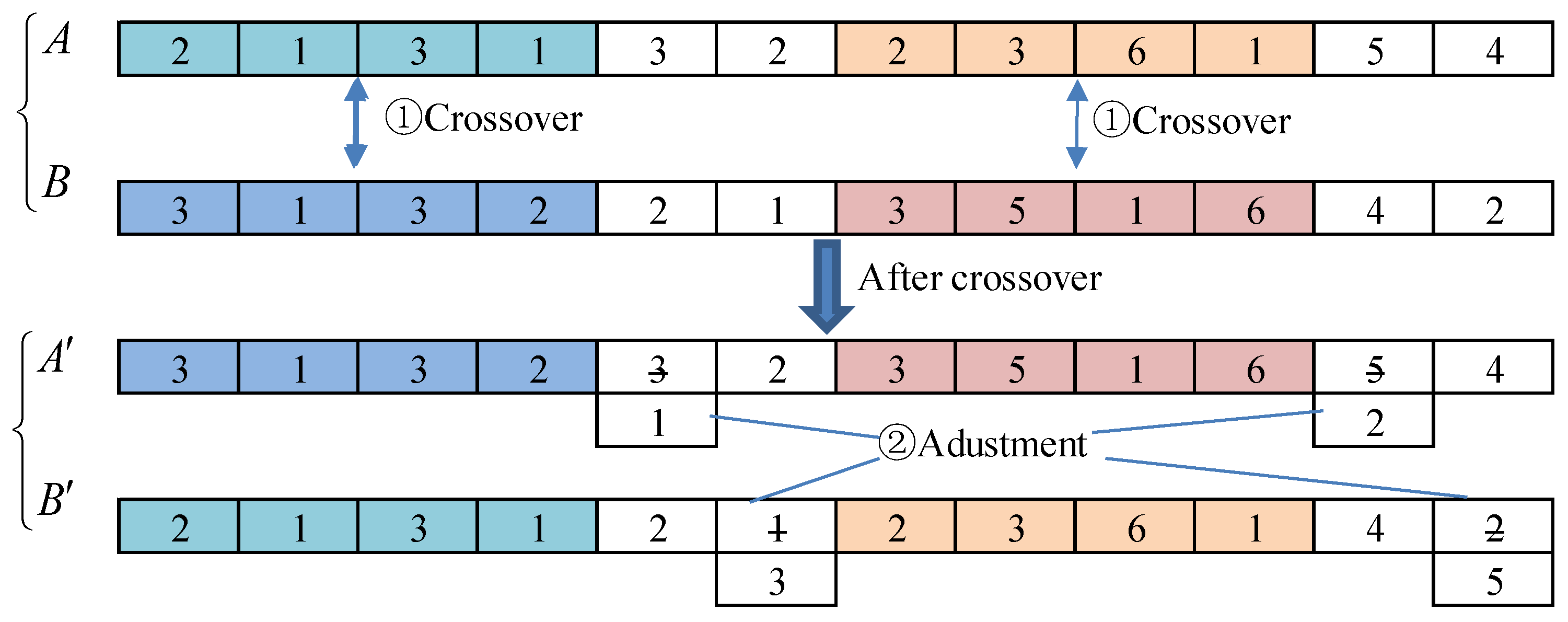
The integer crossover method is used for crossover operations. First, two chromosomes are randomly selected from the population, and the first ${\sum }_{j=1}^N{K}_j$ bits of each chromosome are taken out, and then the intersection positions are randomly selected. After the crossover, the subtasks of some tasks are redundant or missing. Therefore, it is necessary to adjust the redundant subtasks to the missing subtasks and adjust the corresponding services. The crossover operation is shown in Figure 5.

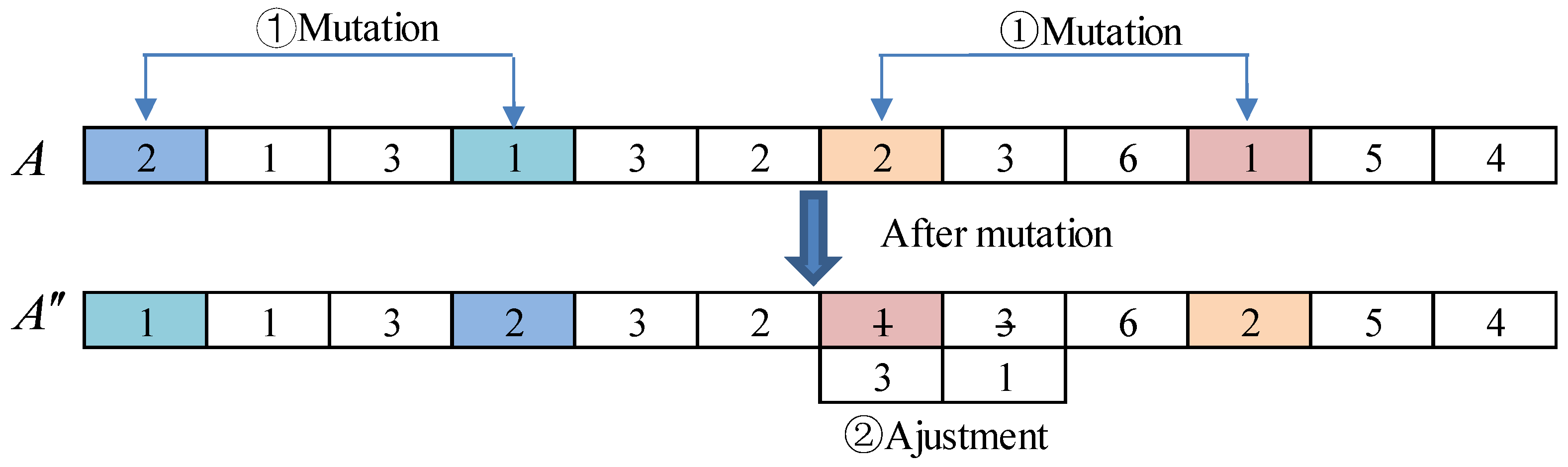
The mutation operator first randomly selects an individual from the population, then randomly selects two mutation bits, and finally exchanges the two subtasks and the corresponding service numbers in the individual. If the modified chromosome does not meet the requirements, adjustments are performed on it. The mutation operation is shown in Figure 6.

4. Computational Experiments and Results

In this section, a small-scale example is first used to illustrate the effect of the proposed method. Then a number of computational experiments with problems of various sizes are designed to demonstrate its effectiveness and efficiency. At last, performance stability of the proposed method is tested.

4.1. A Small-Scale Example

A small-scale SSS problem on a client-centered CMfg platform is built as an example. In this example, we considered 3 enterprises on the platform, each offering two types of services for clients to choose from. At the same time, 4 tasks are accepted, and each task is decomposed into four subtasks that are executed in sequence. The detail parameters of this example are shown in

Table 5. Task and service information.

	$\mathit{S}{\mathit{T}}_{\mathit{j},\mathit{k}}$		$\mathit{S}{\mathit{T}}_{\mathit{j}\mathbf{,}\mathbf{1}}$			$\mathit{S}{\mathit{T}}_{\mathit{j}\mathbf{,}\mathbf{2}}$			$\mathit{S}{\mathit{T}}_{\mathit{j}\mathbf{,}\mathbf{3}}$			$\mathit{S}{\mathit{T}}_{\mathit{j}\mathbf{,}\mathbf{4}}$
${\mathit{T}}_{\mathit{j}}$
$T_1$		$S{E}_{i,h}$	(1,2)	(3,1)	(3,2)	(2,1)	(2,2)	(3,1)	(1,1)	(1,2)	(3,1)	(1,1)	(3,1)	(3,2)
		$st$	9	10	8	5	6	5	7	6	7	7	6	6
		$sc$	55	46	63	67	55	67	67	46	53	43	79	57
		$q$	0.48	0.25	0.16	0.81	0.40	0.32	0.85	0.73	0.96	0.35	0.45	0.33
		$ec$	10	13	6	7	15	13	14	15	14	8	11	12
		$we$	18	19	20	22	17	17	23	16	19	14	19	15
$T_2$		$S{E}_{i,h}$	(1,1)	(1,2)	(3,1)	(1,1)	(1,2)	(3,1)	(1,1)	(1,2)	(2,2)	(1,1)	(3,1)	(3,2)
		$st$	8	7	8	5	8	7	6	5	3	7	3	3
		$sc$	43	65	80	52	47	62	49	70	71	70	48	48
		$q$	0.94	0.48	0.40	0.59	0.60	0.91	0.37	0.53	0.56	0.72	0.25	0.30
		$ec$	9	9	12	5	9	7	13	14	12	14	14	15
		$we$	20	19	11	19	14	15	23	14	18	24	19	27
$T_3$		$S{E}_{i,h}$	(1,2)	(2,2)	(3,1)	(2,2)	(3,1)	(3,2)	(2,2)	(3,1)	(3,2)	(1,1)	(1,2)	(2,2)
		$st$	4	3	6	7	6	5	6	4	5	7	7	7
		$sc$	64	56	45	52	72	49	47	55	60	48	59	44
		$q$	0.72	0.90	0.55	0.48	0.40	0.55	0.26	0.36	0.70	0.73	1.0	0.85
		$ec$	6	14	15	7	13	13	7	6	6	9	5	13
		$we$	12	14	19	21	24	19	27	24	21	24	16	17
$T_4$		$S{E}_{i,h}$	(1,2)	(2,1)	(3,2)	(1,1)	(2,1)	(3,2)	(1,1)	(1,2)	(2,1)	(1,2)	(2,1)	(3,2)
		$st$	5	8	10	4	6	5	3	6	4	6	3	7
		$sc$	63	49	60	65	46	78	79	79	56	67	73	60
		$q$	0.39	0.46	0.16	0.22	0.62	0.50	0.16	0.98	0.36	0.95	0.20	0.75
		$ec$	11	6	11	6	13	15	15	13	13	5	5	8
		$we$	11	11	13	14	22	14	18	25	23	14	21	14

and

Table 6. Geographical distance $d_{i,i^{\prime }}$ between enterprises.

Enterprise	${\mathit{E}}_{\mathbf{1}}$	${\mathit{E}}_{\mathbf{2}}$	${\mathit{E}}_{\mathbf{3}}$
$E_1$	0	125	111
$E_2$	125	0	190
$E_3$	111	190	0

. Table 5 presents the information about tasks and services, such as: alternative services, time, cost, quality, environmental cost and weight of product. For example, the subtask 3 of task 3 could be executed on service $S{E}_{2,2}$, $S{E}_{3,1}$, $S{E}_{3,2}$. If subtask $S{T}_{3,3}$ is assigned to service $S{E}_{2,2}$, then $s{t}_{3,3}^{2,2}=1$, $s{c}_{3,3}^{2,2}=47$, $q_{3,3}^{2,2}=0.26$, $e{c}_{3,3}^{2,2}=7$, $w{e}_{3,3}^{2,2}=27$. The measurement unit of time is days, and the unit of cost is US dollar.

The distance between enterprises is shown in Table 6. For example, $d_{2,3}=190$. The logistics time parameter $\alpha =0.08$, the logistics cost parameter $\beta =0.005$. The measure ment unit for distande is kilometer.

DM considers the four objectives shown in Equations (4)–(7) and each objective has different priority. The priority order of the four objectives is 3-1-2-2, which means that:

Priority level 1: $f_2$,

Priority level 2: $f_3$ and $f_4$,

Priority level 3: $f_1$.

According to Equation (15), the priority relationship can be expressed as

$${\mu }_{f_2}\ge \left({\mu }_{f_3}, {\mu }_{f_4}\right)\ge {\mu }_{f_1}$$

(28)

To verify the effectiveness of the TP-OPS method, two other methods (the max–min method and the FGP method) are adopted for comparison. Then, this example is solved by three methods. In the TP-OPS method, $\Delta \delta$ in Equation (20) is set as 0.9. The max–min method is actually the phase 1 in the TP-OPS method, see Equation (18). The FGP method is to solve Equation (16). In particular, $\epsilon$ is not considered in the max–min method and the FGP method. In order to make a comparative analysis, the optimal ${\mu }_{f_g}$ obtained by these two methods is introduced into Equation (29) to obtain the corresponding $\epsilon$, which is then compared with the result of the TP-OPS method.

$$\{\begin{array}{l}\max \epsilon \hfill \\ {\mu }_{f_g}-{\mu }_{f_{g^{\prime }}}\ge \gamma ,\forall P\left(f_g\right)<P\left(f_{g^{\prime }}\right), g,g^{\prime }=1,2,\cdots ,G\hfill \end{array}$$

(29)

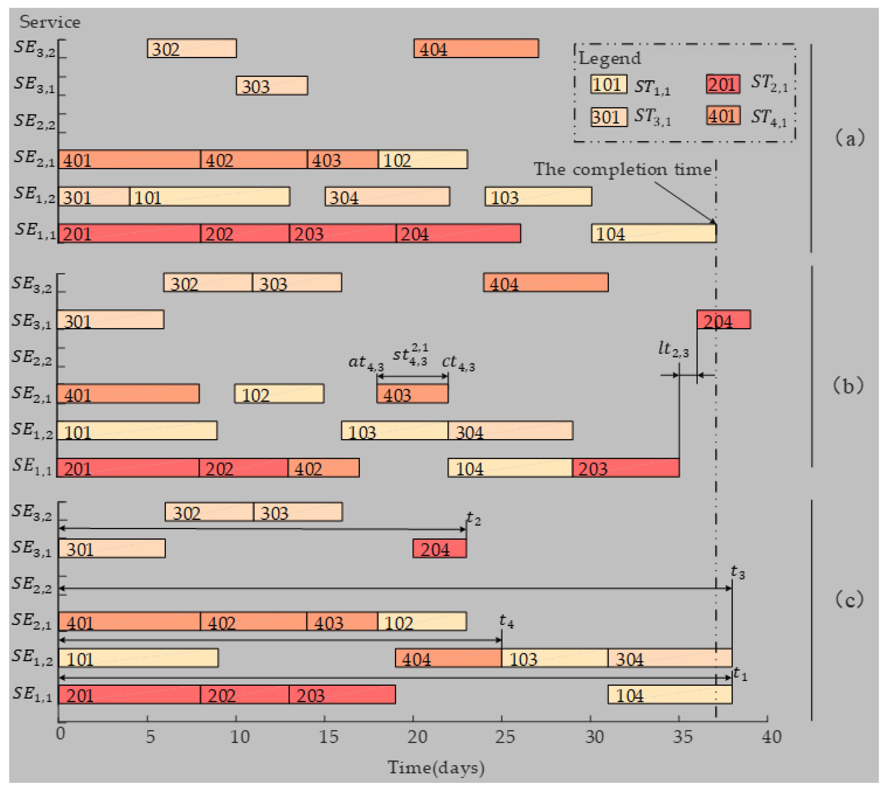
Figure 7 is the Gantt chart of the results for this example found by the three methods. It can be observed that the completion time found by three methods is different. Different methods get different solutions mainly for two reasons. First, FPG method and TP-OPS method consider objective priorities, while max–min method does not. Second, the selection criteria of the optimal solutions of the three methods are different. In this example, the objective about time $f_1$ is the least important. The max–min method does not take into account the different priorities of the objectives, so the corresponding completion time is shorter than the TP-OPS method and the FGP method. Therefore, compared with max–min method, the solutions obtained by FGP method and TP-OPS method can better ensure that important objectives are preferentially satisfied.

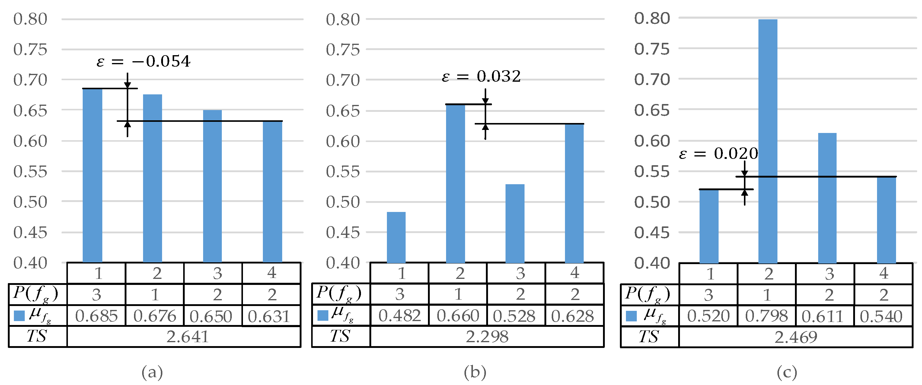
In addition, satisfaction ${\mu }_{f_g}$, priority variable $\epsilon$ and total satisfaction $TS={\sum }_{g=1}^G{\mu }_{f_g}$ of the above three schemes were calculated separately and shown in Figure 8. From this figure, we can see $\epsilon =-0.054<0$ in (a), which means that the satisfactions does not meet priority order 3-1-2-2, and $TS=2.641$ in (a) is the largest of all methods. In Equation (16), the objective function of the FGP method is to maximize $TS$. However due to the priority requirement, $TS=2.469$ in (c) is less than $TS=2.641$ in (a). Compared with (a) and (c), $\epsilon =0.032$ in (b) achieves the maximization of differences in satisfaction between objectives with different priority. Therefore, the results of both TP-OPS method and FGP method can satisfy the priority constraint, but the max–min method could not. In addition, in the case of fixed $\Delta \delta =0.9$, TP-OPS method can obtain $\epsilon$ larger than FGP method. If iterated, TP-OPS method may also achieve a larger $\epsilon$. When DM wants $\epsilon$ to be larger, then TP-OPS method will be more suitable.

In the above result of the TP-OPS method, $\Delta \delta =0.9$. By gradually reducing $\Delta \delta$, different results are obtained by the TP-OPS method and shown in

Table 7. The results found by the TP-OPS method with different $\Delta \delta$ for example 4.1.

$\Delta \mathit{\delta }$	$\mathit{P}\mathbf{\left(}{\mathit{f}}_{\mathit{g}}\mathbf{\right)}$	${\mathit{\mu }}_{{\mathit{f}}_{\mathit{g}}}$	$\mathit{\epsilon }$	$\mathit{T}\mathit{S}$
0.95	[3 1 2 2]	[0.572 0.653 0.590 0.645]	0.016	2.460
0.9	[3 1 2 2]	[0.482 0.660 0.528 0.628]	0.032	2.298
0.85	[3 1 2 2]	[0.534 0.679 0.577 0.601]	0.043	2.388
0.8	[3 1 2 2]	[0.488 0.639 0.566 0.579]	0.060	2.271
0.75	[3 1 2 2]	[0.433 0.631 0.517 0.502]	0.068	2.080
0.7	[3 1 2 2]	[0.475 0.697 0.600 0.586]	0.097	2.356

. It can be found that as $\Delta \delta$ becomes smaller, $\epsilon$ gradually increases, which indicates that the difference in satisfaction between objectives with different priorities is becoming more and more obvious.

When DM considers different priority orders, the satisfactions will also be different. The results found by the TP-OPS method with six different sets of priority orders are shown in

Table 8. The results found by the TP-OPS method with different $P\left(f_g\right)$ for example 4.1.

$\mathit{P}\mathbf{\left(}{\mathit{f}}_{\mathit{g}}\mathbf{\right)}$	$\Delta \mathit{\delta }$	${\mathit{\mu }}_{{\mathit{f}}_{\mathit{g}}}$	$\mathit{\epsilon }$	$\mathit{T}\mathit{S}$
[1 3 3 2]	0.85	[0.633 0.534 0.534 0.579]	0.044	2.280
[2 1 1 3]	0.85	[0.602 0.660 0.676 0.561]	0.041	2.500
[3 2 2 1]	0.85	[0.510 0.548 0.603 0.674]	0.038	2.335
[2 3 1 2]	0.85	[0.578 0.514 0.695 0.561]	0.047	2.348
[3 1 2 1]	0.85	[0.548 0.638 0.595 0.645]	0.042	2.426
[1 2 3 3]	0.85	[0.694 0.648 0.593 0.579]	0.045	2.512

. It can be found that with the change of preference, satisfaction also changes.

From this example, it can be seen that the TP-OPS method has higher flexibility compared to the other two methods. It is still necessary to investigate the performance of problems of different scales; a more detailed analysis is provided in the next section.

4.2. Computational Experiments

4.2.1. Data Generation

The number of services, tasks, and subtasks are selected from three sets, namely $\left\{9,12,15\right\}$, $\left\{6,11,16\right\}$ and $\left\{8,13,18\right\}$. Then $3^3=27$ combinations of problem sizes could be generated, and we chose 9 of them for the experiment, i.e., 9s6t8st, 9s11t13st, 9s16t18st, 12s6t8st, 12s11t13st, 12s16t13st, 15s11t8st, 15s11t13st, 15s16t18st. For each of these combinations, one set of data is randomly generated, in which each parameter is uniform distributed. Their range is shown in

Table 9. The ranges of parameters.

$\mathit{s}\mathit{t}$	$\mathit{s}\mathit{c}$	$\mathit{q}$	$\mathit{e}\mathit{c}$	$\mathit{w}\mathit{e}$	${\mathit{d}}_{\mathit{i},{\mathit{i}}^{\mathbf{\prime }}}$	$\mathit{P}\mathbf{\left(}{\mathit{f}}_{\mathit{g}}\mathbf{\right)}$
[5, 20]	[50, 100]	[0.01, 1]	[10, 30]	[15, 35]	[50, 600]	[1, 3]

. These parameters represent service time ($st$), service cost ($sc$), service quality (q), environmental cost ($ec$), weight of product ($we$), distance between enterprises ($d_{i,i^{\prime }}$) and priority level of objectives ($P\left(f_g\right)$) in turn.

4.2.2. Define GA in Full Term

In this study, we selected 50 individuals per generation, performed 100 iterations with a crossover probability of 0.8 and a mutation probability of 0.1, which has been used in our previous research on SSS problem. For each selected question, statistical results for ten runs were obtained and shown in the following subsection for each method. For the TP-OPS method, two cases ($\Delta \delta =0.9$ and $\Delta \delta =0.7$) are considered to preliminarily observe the effect of Δδ on results. All algorithms are implemented in Matlab software.

4.2.3. Test Results

The following performance indicators are considered:

${\mu }_{min}=min\left(\mu \left(f_g\right)\right)\left(g=1,2,\cdots ,G\right)$: the minimum satisfaction of all objectives, representing the optimization of the least important objectives. The mean and standard deviation of ${\mu }_{min}$ for 10 runs are denoted as $\overline{{\mu }_{min}}$ and $S_{{\mu }_{min}}$.

$\epsilon$: priority variable, which means the difference in satisfaction between objectives with different priority. The mean and standard deviation of $\epsilon$ for 10 runs is denoted as $\overline{\epsilon }$ and $S_{\epsilon }$.

$TS={\sum }_{g=1}^G{u}_{f_g}$: total satisfaction, which means the optimization of all objectives. The mean and standard deviation of $TS$ for ten runs is denoted as $\overline{TS}$ and $S_{TS}$.

$NFS$: the number of times that a feasible solution satisfying priority constraints is found in 10 runs. For example, If the optimal solution found by the max–min method satisfies constraint (15) in a certain run, then $NFS=NFS+1$, otherwise, it is not included in $NFS$. Similarly, if $\epsilon >0$, it also means that constraint (15) is satisfied and counted in $NFS$.

$NFS$ for 10 runs obtained by different methods are shown in

Table 10. $NFS$ for 10 runs obtained by different methods.

Dataset	Max–Min	TP-OPS		FGP
		$\Delta \mathit{\delta }\mathbf{=}\mathbf{0.9}$	$\Delta \mathit{\delta }\mathbf{=}\mathbf{0.7}$
9s6t8st	3	10	10	10
9s11t13st	1	8	10	10
9s16t18st	0	9	10	10
12s6t8st	0	8	10	10
12s11t13st	0	10	10	10
12s16t13st	1	10	10	10
15s11t8st	1	10	10	10
15s11t13st	1	10	10	10
15s16t18st	0	10	10	10

. For the max–min method, the optimal solution can only satisfy priority constraint (15) by a small random probability, so most $\epsilon$ obtained by Equation (29) is less than 0. For the TP-OPS method, when $\Delta \delta =0.9$, the search space is not large enough, resulting in $NFS<10$. When $\Delta \delta =0.7$, feasible solutions are found for each run, and $NFS=10$. For the FGP method, feasible solutions are found for each run and each combination. Therefore, both TP-OPS method and FGP method can meet the requirements in finding feasible solutions satisfying priority constraints. But TP-OPS method may need to reduce $\Delta \delta$ in phase 2, for example $\Delta \delta$ changes from 0.9 to 0.7 in Table 10. It needs to be noted that statistical results refer to the feasible solutions counted in $NFS$.

The mean and standard deviation of ${\mu }_{min}$ for 10 runs obtained by three method are summarized in

Table 11. Mean and standard deviation of ${\mu }_{min}$ for 10 runs obtained by different methods.

Dataset	Max–Min		TP-OPS				FGP
	$\overline{{\mathit{\mu }}_{\mathit{m}\mathit{i}\mathit{n}}}$	${\mathit{S}}_{{\mathit{\mu }}_{\mathit{m}\mathit{i}\mathit{n}}}$	$\Delta \mathit{\delta }=0.9$		$\Delta \mathit{\delta }=0.7$		$\overline{{\mathit{\mu }}_{\mathit{m}\mathit{i}\mathit{n}}}$	${\mathit{S}}_{{\mathit{\mu }}_{\mathit{m}\mathit{i}\mathit{n}}}$
			$\overline{{\mathit{\mu }}_{\mathit{m}\mathit{i}\mathit{n}}}$	${\mathit{S}}_{{\mathit{\mu }}_{\mathit{m}\mathit{i}\mathit{n}}}$	$\overline{{\mathit{\mu }}_{\mathit{m}\mathit{i}\mathit{n}}}$	${\mathit{S}}_{{\mathit{\mu }}_{\mathit{m}\mathit{i}\mathit{n}}}$
9s6t8st	0.536	0.030	0.467	0.030	0.397	0.027	0.482	0.058
9s11t13st	0.433	0.036	0.395	0.036	0.329	0.038	0.258	0.092
9s16t18st	0.463	0.030	0.426	0.023	0.362	0.028	0.340	0.119
12s6t8st	0.527	0.025	0.472	0.035	0.421	0.044	0.402	0.093
12s11t13st	0.505	0.033	0.441	0.035	0.391	0.028	0.425	0.059
12s16t13st	0.514	0.041	0.463	0.040	0.368	0.030	0.420	0.065
15s11t8st	0.493	0.044	0.434	0.039	0.365	0.035	0.374	0.075
15s11t13st	0.471	0.040	0.412	0.036	0.353	0.023	0.390	0.053
15s16t18st	0.483	0.042	0.428	0.040	0.359	0.032	0.403	0.056

. It can be seen from the table that for any combination, $\overline{{\mu }_{min}}$ of TP-OPS method is less than that of the max–min method. The objectives of the max–min method and phase 1 of TP-OPS method are both to maximize ${\mu }_{min}$, so $\overline{{\mu }_{min}}$ of the max–min method is the limit value of TP-OPS method. For the FGP method, $\overline{{\mu }_{min}}$ is smaller than that of the max–min method, but this gap seems to remain within a certain level, because too small ${\mu }_{min}$ is not conducive to maximize $TS$.

Table 12. Mean and standard deviation of $\epsilon$ for ten runs obtained by different methods.

Dataset	Max–Min		TP-OPS				FGP
	$\overline{\mathit{\epsilon }}$	${\mathit{S}}_{\mathit{\epsilon }}$	$\Delta \mathit{\delta }=0.9$		$\Delta \mathit{\delta }=0.7$		$\overline{\mathit{\epsilon }}$	${\mathit{S}}_{\mathit{\epsilon }}$
			$\overline{\mathit{\epsilon }}$	${\mathit{S}}_{\mathit{\epsilon }}$	$\overline{\mathit{\epsilon }}$	${\mathit{S}}_{\mathit{\epsilon }}$
9s6t8st	0.014	0.015	0.076	0.032	0.143	0.019	0.037	0.026
9s11t13st	0.001	0.000	0.033	0.020	0.073	0.023	0.106	0.071
9s16t18st	-	-	0.023	0.013	0.057	0.023	0.071	0.039
12s6t8st	-	-	0.031	0.017	0.055	0.014	0.032	0.024
12s11t13st	-	-	0.037	0.012	0.084	0.019	0.036	0.025
12s16t13st	0.005	0.000	0.047	0.020	0.103	0.025	0.070	0.048
15s11t8st	0.001	0.000	0.031	0.018	0.064	0.027	0.070	0.063
15s11t13st	0.005	0.000	0.032	0.013	0.066	0.014	0.065	0.025
15s16t18st	-	-	0.028	0.012	0.066	0.020	0.047	0.024

shows the results of $\overline{\epsilon }$ and $S_{\epsilon }$ for the three methods, in which “-” means all $\epsilon <0$. It can be seen that for different combinations, $\overline{\epsilon }$ of the max–min method is the smallest due to the neglect of priority. For the TP-OPS method, the limitation of search space leads to smaller $\overline{\epsilon }$ when $\Delta \delta =0.9$. By adjusting $\Delta \delta$ to 0.7, the broader search space also makes $\overline{\epsilon }$ larger. For the FGP method, $\overline{\epsilon }$ is sometimes larger than TP-OPS $\Delta \delta =0.7$ (such as: combination 9s11t13st), and sometimes smaller than TP-OPS $\Delta \delta =0.9$ (such as: combination 9s6t8st). This instability is not conducive to DM’s judgment on the appropriateness of the current result.

In terms of $TS$, the FGP method has an advantage because its objective function is to maximize $TS$. For three methods, $\overline{TS}$ and $S_{TS}$ are summarized in

Table 13. Mean and standard deviation of $TS$ for 10 runs obtained by different methods.

Dataset	Max–Min		TP-OPS				FGP
	$\overline{\mathit{T}\mathit{S}}$	${\mathit{S}}_{\mathit{T}\mathit{S}}$	$\Delta \mathit{\delta }=0.9$		$\Delta \mathit{\delta }=0.7$		$\overline{\mathit{T}\mathit{S}}$	${\mathit{S}}_{\mathit{T}\mathit{S}}$
			$\overline{\mathit{T}\mathit{S}}$	${\mathit{S}}_{\mathit{T}\mathit{S}}$	$\overline{\mathit{T}\mathit{S}}$	${\mathit{S}}_{\mathit{T}\mathit{S}}$
9s6t8st	2.261	0.121	2.211	0.128	2.117	0.083	2.569	0.102
9s11t13st	1.833	0.156	1.783	0.148	1.632	0.189	2.055	0.153
9s16t18st	2.000	0.160	1.897	0.147	1.770	0.090	2.022	0.175
12s6t8st	2.218	0.096	2.074	0.168	1.961	0.136	2.144	0.152
12s11t13st	2.102	0.142	2.005	0.140	1.923	0.132	2.276	0.115
12s16t13st	2.158	0.179	2.084	0.173	1.915	0.176	2.466	0.106
15s11t8st	2.077	0.159	1.948	0.133	1.833	0.140	2.158	0.128
15s11t13st	1.952	0.192	1.909	0.175	1.870	0.127	2.229	0.125
15s16t18st	2.041	0.192	1.920	0.160	1.776	0.166	2.164	0.120

. It can be seen from this table that for most combinations, $\overline{TS}$ of FGP method is still the largest of the three methods, although an exception has occurred for combination 12s6t8st. This phenomenon that $TS$ of FPG method is smaller than the max–min method in some individual case (which can also be seen in Figure 8) is mainly due to the influence of the constraint (15). Both TP-OPS method and the max–min method focus on maximizing ${\mu }_{min}$ without paying attention to the highest priority objective, so it is not easy to make individual satisfaction particularly high like FGP method shown in Figure 3c. In addition, compared to the max–min method, TP-OPS method performs the optimization of phase 2 according to Equation (20), which further affects $\overline{TS}$.

Figure 9 shows the mean CPU time for 10 runs obtained by different methods. It can be seen that the CPU time of three methods is affected by the scale of the problem. The larger the scale, the more time it takes. Here, $t_{p2}^{0.7}$ and $t_{p2}^{0.9}$ indicate the time consumed by phase 2 when $\Delta \delta =0.7$ and $\Delta \delta =0.9$ respectively. Then it can be seen from Figure 9 that in all combinations, $t_{p2}^{0.7}$ and $t_{p2}^{0.9}$ both are much smaller than the time of the max–min method.

The effects of $\Delta \delta$ on results is tested on a selected data set, i.e., 12t11s18st. For each different $\Delta \delta$ from 0.95 to 0.7, TP-OPS method runs 10 times.

Table 14. Mean of performance indicators for 10 runs found by TP-OPS method with different $\Delta \mathsf{\delta }$.

$\Delta \mathit{\delta }$	$\mathit{P}\left({\mathit{f}}_{\mathit{g}}\right)$	$\overline{{\mathit{u}}_{{\mathit{f}}_1}}$	$\overline{{\mathit{u}}_{{\mathit{f}}_2}}$	$\overline{{\mathit{u}}_{{\mathit{f}}_3}}$	$\overline{{\mathit{u}}_{{\mathit{f}}_4}}$	$\overline{\mathit{\epsilon }}$	$\overline{\mathit{T}\mathit{S}}$	$\mathit{N}\mathit{F}\mathit{S}$
0.95	[2 1 3 1]	0.484	0.460	0.432	0.445	0.009	1.821	2
0.9	[2 1 3 1]	0.452	0.480	0.423	0.466	0.018	1.821	6
0.85	[2 1 3 1]	0.452	0.499	0.428	0.507	0.020	1.886	10
0.8	[2 1 3 1]	0.475	0.543	0.424	0.523	0.031	1.965	10
0.75	[2 1 3 1]	0.424	0.500	0.366	0.483	0.041	1.773	10
0.7	[2 1 3 1]	0.440	0.524	0.369	0.547	0.059	1.880	10

shows the mean of performance indicators found with different $\Delta \delta$. As can be seen from this table that as $\Delta \delta$ becomes smaller, the satisfactions of high priority objectives ($u_{f_2}$ and $u_{f_4}$) tend to increase, while the satisfaction of low priority objective ($u_{f_3}$) gradually decreases. This leads to the gradual increase of $\epsilon$. However, with the change of $\Delta \delta$, $TS$ has no obvious change trend and is relatively stable in a certain range. In addition, the smaller the $\Delta \delta$, the larger the $NFS$.

The effects of $P\left(f_g\right)$ on results is also tested on the selected data set (i.e., 12t11s18st), and six priority orders are considered. For each priority order, TP-OPS method also runs ten times. The following can be found in

Table 15. Mean of performance indicators for 10 runs found by TP-OPS method with different $P\left(f_g\right)$.

Case	$\mathit{P}\left({\mathit{f}}_{\mathit{g}}\right)$	$\overline{\Delta \mathit{\delta }}$	$\overline{{\mathit{u}}_{{\mathit{f}}_1}}$	$\overline{{\mathit{u}}_{{\mathit{f}}_2}}$	$\overline{{\mathit{u}}_{{\mathit{f}}_3}}$	$\overline{{\mathit{u}}_{{\mathit{f}}_4}}$	$\overline{\mathit{\epsilon }}$	$\overline{\mathit{T}\mathit{S}}$	$\mathit{N}\mathit{F}\mathit{S}$
1	[1 3 3 2]	0.85	0.607	0.448	0.440	0.507	0.047	2.002	10
2	[2 1 1 3]	0.85	0.446	0.466	0.454	0.385	0.020	1.751	9
3	[3 2 2 1]	0.85	0.461	0.481	0.470	0.507	0.014	1.919	8
4	[2 3 1 2]	0.85	0.484	0.433	0.521	0.472	0.024	1.910	10
5	[3 1 2 1]	0.85	0.465	0.505	0.478	0.505	0.017	1.953	8
6	[1 2 3 3]	0.85	0.601	0.519	0.441	0.450	0.062	2.011	10

. $\overline{\epsilon }$ is relative larger when there are more low priority objectives (cases 1 and 6) than when there are more high priority objectives (cases 2 and 5). A smaller mean of $\epsilon$ represents an increase in the probability that $\epsilon <0$. $u_{f_g}$ is affected not only by its own priority $P\left(f_g\right)$, but also by priorities of other objective. For example, $P\left(f_1\right)=2$ in case 2 and $P\left(f_1\right)=3$ in case 3, however $0.446<0.461$.

4.3. Applicability of Different Methods

In order to test the applicability of different methods, we increase the number of services, tasks and subtasks in this section. In addition, different number of objectives and priority levels are also considered.

4.3.1. Different Scales of Services and Tasks/Subtasks

In this subsection, the number of services increases from [9, 12, 15] to [300, 600, 900], the number of tasks from [6, 11, 16] to [16, 30, 50], and the number of subtasks from [8, 13, 18] to [18, 50]. The ranges of other parameters follow the data in Table 9. Each dataset is also tested 10 times. The averages of ${\mu }_{min}$, $\epsilon$, $\mathit{TS}$, CPU time for 10 runs are computed respectively, and the test results of different methods are summarized in

Table 16. $\overline{{\mu }_{min}}$, $\overline{\epsilon }$, $\overline{TS}$ obtained by different methods for larger scale problems.

Dataset	Max–Min			TP-OPS						FGP
	$\overline{{\mathit{\mu }}_{\mathit{m}\mathit{i}\mathit{n}}}$	$\overline{\mathit{\epsilon }}$	$\overline{\mathit{T}\mathit{S}}$	$\Delta \mathit{\delta }=0.85$			$\Delta \mathit{\delta }=0.7$			$\overline{{\mathit{\mu }}_{\mathit{m}\mathit{i}\mathit{n}}}$	$\overline{\mathit{\epsilon }}$	$\overline{\mathit{T}\mathit{S}}$
				$\overline{{\mathit{\mu }}_{\mathit{m}\mathit{i}\mathit{n}}}$	$\overline{\mathit{\epsilon }}$	$\overline{\mathit{T}\mathit{S}}$	$\overline{{\mathit{\mu }}_{\mathit{m}\mathit{i}\mathit{n}}}$	$\overline{\mathit{\epsilon }}$	$\overline{\mathit{T}\mathit{S}}$
300s16t18st	0.431	-	1.872	0.392	0.001	1.739	0.330	0.034	1.617	0.326	0.058	1.717
600s16t18st	0.431	-	1.874	0.386	0.015	1.734	0.330	0.041	1.647	0.305	0.044	1.623
900s16t18st	0.516	-	2.226	0.459	0.026	2.111	0.380	0.067	2.021	0.405	0.037	2.126
900s30t18st	0.512	-	2.232	0.456	0.018	2.035	0.399	0.033	1.890	0.313	0.027	1.649
900s16t50st	0.491	-	2.086	0.432	0.018	1.890	0.369	0.054	1.781	0.351	0.026	1.813
900s50t50st	0.458	-	1.962	0.418	0.020	1.873	0.358	0.053	1.725	0.343	0.059	1.903

. From this table, it can be seen that: when the number of services increases from 300 to 900, both $\overline{{\mu }_{min}}$ and $\overline{TS}$ have an increasing trend, which shows that the more services, the better the clients’ needs can be met. When the number of services remains at 900 and the number of tasks/subtasks increases, $\overline{{\mu }_{min}}$ and $\overline{TS}$ have a tendency to decrease, which shows that clients’ satisfaction will also be reduced if resources are limited. In addition, some of the statistical results also have some deviations from this trend, mainly due to the random generation of data. For large-scale problems, the TP method can still obtain reasonable results. From the perspective of $\overline{\epsilon }$, the max–min method can hardly produce solutions satisfying priority constraints for larger-scale problems, while TP-OPS method can still get reasonable results.

The CPU time of all methods increases with the number of services and tasks/subtasks, as shown in Figure 10. As can be seen from the figure, the change in CPU time caused by the increase in the number of services from 300 to 900 is much smaller than the increase in the number of tasks and subtasks from 16t18st to 50t50st. Faced with the task flow of additional tasks in and released products out in dynamic market, this paper chooses to treat a decision period as static, so fast decision-making is very important. For FGP method, If DM is not satisfied with the results, recalculation will consume a lot of time. Compared with the FGP method, the TP-OPS method has advantages, and only requires less time to adjust $\Delta \delta$.

4.3.2. Different Number of Objectives and Priority Levels

For most multi-objective optimization problems in manufacturing, the number of objectives is usually between 2 and 4. In the previous small-scale example and computational experiments, four objectives and three priority levels were considered, i.e., the number of objectives $G=4$, the number of priority levels $L=3$. Therefore, further experiments are necessary to test the effects of different $G$ and $L$ on the results. In this subsection, we chose the common situation, where $G\in \left[2, 3, 4\right], L\in \left[2, 3, 4\right], L\le G$. Combination 18s4t15st is selected for the experiment, and other parameters are the same as Table 9. The test results are summarized in

Table 17. Performance stability of different methods for different scales.

G	L	Max–Min			TP-OPS						FGP
		$\mathit{N}\mathit{F}\mathit{S}$	$\overline{{\mathit{\mu }}_{\mathit{m}\mathit{i}\mathit{n}}}$	$\overline{\mathit{\epsilon }}$	$\Delta \mathit{\delta }=0.85$			$\Delta \mathit{\delta }=0.7$			$\mathit{N}\mathit{F}\mathit{S}$	$\overline{{\mathit{\mu }}_{\mathit{m}\mathit{i}\mathit{n}}}$	$\overline{\mathit{\epsilon }}$
					$\mathit{N}\mathit{F}\mathit{S}$	$\overline{{\mathit{\mu }}_{\mathit{m}\mathit{i}\mathit{n}}}$	$\overline{\mathit{\epsilon }}$	$\mathit{N}\mathit{F}\mathit{S}$	$\overline{{\mathit{\mu }}_{\mathit{m}\mathit{i}\mathit{n}}}$	$\overline{\mathit{\epsilon }}$
2	2	5	0.879	0.020	10	0.773	0.120	10	0.643	0.230	10	0.854	0.059
3	2	3	0.804	0.022	10	0.701	0.132	10	0.585	0.249	10	0.739	0.078
3	3	1	0.654	0.001	10	0.580	0.036	10	0.486	0.085	10	0.569	0.034
4	2	3	0.519	0.008	10	0.452	0.081	10	0.386	0.153	10	0.398	0.140
4	3	1	0.519	0.004	9	0.466	0.018	10	0.377	0.044	10	0.360	0.035
4	4	1	0.509	0.012	9	0.455	0.017	10	0.384	0.031	10	0.278	0.023

and it can be seen that the TP-OPS method is applicable for these selected $G$ and $L$, and the conclusions drawn in the previous sections are still valid. It can also be found that the larger $G$ and $L$, the smaller $\overline{{\mu }_{min}}$ and $\overline{\epsilon }$ are. In this paper, we do not consider $G>4$, mainly for two reasons. On the one hand, this situation rarely occurs in the actual manufacturing process. On the other hand, if $\overline{{\mu }_{min}}$ and $\overline{\epsilon }$ become too small, the effect of any optimization method will not be obvious. Therefore, the TP-OPS method is suitable for multi-objective optimization problem which need to achieve the optimization of all objectives, while maximizing the difference in optimization effects among objectives of different importance.

5. Conclusions

This paper proposes a two-phase method based on the order of priority satisfaction (TP-OPS) for the service selection and scheduling problem with different objective priorities in cloud manufacturing. In the proposed method, the order of priority satisfaction is introduced to represent priority requirements of different objectives. As a very convenient method, the TP-OPS only requires decision maker to judge whether the current solution is satisfactory and give the parameters for the next optimization decision. By relaxing the maximum comprehensive satisfaction, the difference between satisfaction of objectives with different priority is gradually expanded. Furthermore, TP-OPS method can achieve a balance between the improvement of maximum comprehensive satisfaction and the control of satisfaction differences. In addition, just a short time is needed to find a new solution after adjusting the parameters, which saves a lot of time for the decision process of large-scale problems. and the method could be applied to small and medium-sized market environments. The TP-OPS proposed in this paper can be applied to many kinds of cloud platforms, such as automobile manufacturing, clothing customization, aerospace and so on. The decision-maker can select a satisfactory solution only by determining objective priorities according to the status of resources and tasks on the platform.

Further research can consider the following two directions. First, other types of satisfaction could be taken into account. For the simplification of calculation, this paper considers that all satisfactions of clients are linear. However, in reality, many clients’ satisfactions show curves or discount forms. Therefore, how to coordinate these different types of clients has become a meaningful research direction. In addition, dynamic and static combination approaches should be designed to adapt to rapid changes in the market. This paper considers the market as static within a certain decision period. However, when faced with the flow of additional tasks in and released products out, centralized optimization and rapid response are essential. So dynamic and static combination approaches will also become a very important research direction.

References

- Xu, X. From cloud computing to cloud manufacturing. Robot. Comput. Int. Manuf. 2012, 28, 75–86. [Google Scholar] [CrossRef]
- He, W.; Xu, L. A state-of-the-art survey of cloud manufacturing. Int. J. Comput. Integr. Manuf. 2015, 28, 239–250. [Google Scholar] [CrossRef]
- Wu, D.; Greer, M.J.; Rosen, D.W.; Schaefer, D. Cloud manufacturing: Strategic vision and state-of-the-art. J. Manuf. Syst. 2013, 32, 564–579. [Google Scholar] [CrossRef] [Green Version]
- Zhang, L.; Mai, J.; Tao, F.; Luo, Y.; Ren, L. Development Status of Cloud Manufacturing in China. In ASME 2014 International Manufacturing Science and Engineering Conference collocated with the JSME 2014 International Conference on Materials and Processing and the 42nd North American Manufacturing Research Conference, Detroit, MI, USA, 9–13 June 2014; AMER SOC MECHANICAL ENGINEERS: New York, NY, USA, 2014. [Google Scholar]
- Ren, L.; Zhang, L.; Tao, F.; Zhao, C.; Chai, X.; Zhao, X. Cloud manufacturing: From concept to practice. Enterp. Inf. Syst. UK 2015, 9, 186–209. [Google Scholar] [CrossRef]
- Ren, L.; Zhang, L.; Wang, L.; Tao, F.; Chai, X. Cloud manufacturing: Key characteristics and applications. Int. J. Comput. Integr. Manuf. 2017, 30, 501–515. [Google Scholar] [CrossRef]
- Akbaripour, H.; Houshmand, M.; van Woensel, T.; Mutlu, N. Cloud manufacturing service selection optimization and scheduling with transportation considerations: Mixed-integer programming models. Int. J. Adv. Manuf. Technol. 2018, 95, 43–70. [Google Scholar] [CrossRef]
- Tao, F.; LaiLi, Y.; Xu, L.; Zhang, L. FC-PACO-RM: A Parallel Method for Service Composition Optimal-Selection in Cloud Manufacturing System. IEEE Trans. Ind. Inf. 2013, 9, 2023–2033. [Google Scholar] [CrossRef]
- Liu, Y.; Xu, X.; Zhang, L.; Wang, L.; Zhong, R.Y. Workload-based multi-task scheduling in cloud manufacturing. Robot. Comput. Int. Manuf. 2017, 45, 3–20. [Google Scholar] [CrossRef]
- Li, F.; Liao, T.W.; Zhang, L. Two-level multi-task scheduling in a cloud manufacturing environment. Robot. Comput. Int. Manuf. 2019, 56, 127–139. [Google Scholar] [CrossRef]
- Argoneto, P.; Renna, P. Supporting capacity sharing in the cloud manufacturing environment based on game theory and fuzzy logic. Enterp. Inf. Syst. UK 2016, 10, 193–210. [Google Scholar] [CrossRef]
- Liu, Y.; Zhang, L.; Tao, F.; Wang, L. Resource service sharing in cloud manufacturing based on the Gale-Shapley algorithm: Advantages and challenge. Int. J. Comput. Integr. Manuf. 2017, 30, 420–432. [Google Scholar] [CrossRef]
- Tao, F.; Zhang, L.; Liu, Y.; Cheng, Y.; Wang, L.; Xu, X. Manufacturing Service Management in Cloud Manufacturing: Overview and Future Research Directions. J. Manuf. Sci. Eng. 2015, 137. [Google Scholar] [CrossRef]
- Xiang, F.; Hu, Y.; Yu, Y.; Wu, H. QoS and energy consumption aware service composition and optimal-selection based on Pareto group leader algorithm in cloud manufacturing system. Cent. Eur. J. Oper. Res. 2014, 22, 663–685. [Google Scholar] [CrossRef]
- Liu, W.; Liu, B.; Sun, D.; Li, Y.; Ma, G. Study on multi-task oriented services composition and optimisation with the “Multi-Composition for Each Task’ pattern in cloud manufacturing systems. Int. J. Comput. Integr. Manuf. 2013, 26, 786–805. [Google Scholar] [CrossRef]
- Huang, B.; Li, C.; Tao, F. A chaos control optimal algorithm for QoS-based service composition selection in cloud manufacturing system. Enterp. Inf. Syst. UK 2014, 8, 445–463. [Google Scholar] [CrossRef]
- Cheng, Y.; Tao, F.; Liu, Y.; Zhao, D.; Zhang, L.; Xu, L. Energy-aware resource service scheduling based on utility evaluation in cloud manufacturing system. Proc. Inst. Mech. Eng. Part B J. Eng. Manuf. 2013, 227, 1901–1915. [Google Scholar] [CrossRef]
- Zhou, J.; Yao, X. Multi-objective hybrid artificial bee colony algorithm enhanced with Lévy flight and self-adaption for cloud manufacturing service composition. Appl. Intell. 2017, 47, 721–742. [Google Scholar] [CrossRef]
- Zhou, J.; Yao, X. A hybrid approach combining modified artificial bee colony and cuckoo search algorithms for multi-objective cloud manufacturing service composition. Int. J. Prod. Res. 2017, 55, 4765–4784. [Google Scholar] [CrossRef]
- Cao, Y.; Wang, S.; Kang, L.; Gao, Y. A TQCS-based service selection and scheduling strategy in cloud manufacturing. Int. J. Adv. Manuf. Tech. 2016, 82, 235–251. [Google Scholar] [CrossRef]
- Yan, K.; Cheng, Y.; Tao, F. A trust evaluation model towards cloud manufacturing. Int. J. Adv. Manuf. Technol. 2016, 84, 133–146. [Google Scholar] [CrossRef]
- Tao, F.; Zhao, D.; Hu, Y.; Zhou, Z. Correlation-aware resource service composition and optimal-selection in manufacturing grid. Eur. J. Oper. Res. 2010, 201, 129–143. [Google Scholar] [CrossRef]
- Li, Y.; Yao, X.; Zhou, J. Multi-objective Optimization of Cloud Manufacturing Service Composition with Cloud-Entropy Enhanced Genetic Algorithm. Stroj. Vestn. J. Mech. Eng. 2016, 62, 577–590. [Google Scholar] [CrossRef]
- Zhou, J.; Yao, X.; Lin, Y.; Chan, F.T.S.; Li, Y. An adaptive multi-population differential artificial bee colony algorithm for many-objective service composition in cloud manufacturing. Inf. Sci. 2018, 456, 50–82. [Google Scholar] [CrossRef] [Green Version]
- Yuan, M.; Deng, K.; Chaovalitwongse, W.A.; Cheng, S. Multi-objective optimal scheduling of reconfigurable assembly line for cloud manufacturing. Optim. Method. Softw. 2017, 32, 581–593. [Google Scholar] [CrossRef]
- Chen, J.; Huang, G.Q.; Wang, J.; Yang, C. A cooperative approach to service booking and scheduling in cloud manufacturing. Eur. J. Oper. Res. 2019, 273, 861–873. [Google Scholar] [CrossRef]
- Laili, Y.; Tao, F.; Zhang, L.; Sarker, B.R. A study of optimal allocation of computing resources in cloud manufacturing systems. Int. J. Adv. Manuf. Technol. 2012, 63, 671–690. [Google Scholar] [CrossRef]
- Chen, F.; Dou, R.; Li, M.; Wu, H. A flexible QoS-aware Web service composition method by multi-objective optimization in cloud manufacturing. Comput. Ind. Eng. 2016, 99, 423–431. [Google Scholar] [CrossRef]
- He, W.; Jia, G.; Zong, H.; Kong, J. Multi-Objective Service Selection and Scheduling with Linguistic Preference in Cloud Manufacturing. Sustainability 2019, 11, 2619. [Google Scholar] [CrossRef]
- Khosravani, S.; Jalali, M.; Khajepour, A.; Kasaiezadeh, A.; Chen, S.; Litkouhi, B. Application of Lexicographic Optimization Method to Integrated Vehicle Control Systems. IEEE Trans. Ind. Electron. 2018, 65, 9677–9686. [Google Scholar] [CrossRef]
- Liu, G.; Shi, L.; Li, K.W. Equitable Allocation of Blue and Green Water Footprints Based on Land-Use Types: A Case Study of the Yangtze River Economic Belt. Sustainability 2018, 10, 3556. [Google Scholar] [CrossRef]
- Chen, L.H.; Tsai, F.C. Fuzzy goal programming with different importance and priorities. Eur. J. Oper. Res. 2001, 133, 548–556. [Google Scholar] [CrossRef]
- Li, S.; Hu, C. Two-step interactive satisfactory method for fuzzy multiple objective optimization with preemptive priorities. IEEE Trans. Fuzzy Syst. 2007, 15, 417–425. [Google Scholar] [CrossRef]
- Khorram, E.; Nozari, V. Multi-objective optimization with preemptive priority subject to fuzzy relation equation constraints. Iran J. Fuzzy Syst. 2012, 9, 27–45. [Google Scholar]
Figure 1.
The abstract model of service selection and scheduling (SSS) in CMfg.
Figure 2.
The schematic diagram of TP-OPS method in the two-objective example. (a) Phase 1 (b) Phase 2 (c) Phase 3.
Figure 3.
Framework of the three SSS methods.
Figure 4.
Schematic diagram of coding.
Figure 5.
The crossover operation.
Figure 6.
The mutation operation.
Figure 7.
Gantt chart of the results for the problem found by (a) the Max–min method (b) the TP-OPS method (c) the FGP method for example 4.1.
Figure 8.
The satisfaction corresponding to the results found by (a) the Max–min method (b) the TP-OPS method (c) the FGP method for example 4.1.
Figure 9.
Mean of CPU time for 10 runs obtained by different methods.
Figure 10.
Mean of CPU time for 10 runs obtained by different methods for larger scale problems.