Lane-Level Road Network Generation Techniques for Lane-Level Maps of Autonomous Vehicles: A Survey


1
State Key Laboratory of Information Engineering in Surveying, Mapping, and Remote Sensing, Wuhan University, Wuhan 430079, China
2
Engineering Research Center for Spatio-Temporal Data Smart Acquisition and Application, Ministry of Education of China, Beijing 100816, China
3
Three Gorges Geotechnical Consultants Co., Ltd. Wuhan, Hubei 430074, China
*
Author to whom correspondence should be addressed.
Sustainability 2019, 11(16), 4511; https://doi.org/10.3390/su11164511
Submission received: 9 July 2019
/
Revised: 16 August 2019
/
Accepted: 16 August 2019
/
Published: 20 August 2019
(This article belongs to the Special Issue Sustainable and Intelligent Transportation Systems)
Abstract
:Autonomous driving is experiencing rapid development. A lane-level map is essential for autonomous driving, and a lane-level road network is a fundamental part of a lane-level map. A large amount of research has been performed on lane-level road network generation based on various on-board systems. However, there is a lack of analysis and summaries with regards to previous work. This paper presents an overview of lane-level road network generation techniques for the lane-level maps of autonomous vehicles with on-board systems, including the representation and generation of lane-level road networks. First, sensors for lane-level road network data collection are discussed. Then, an overview of the lane-level road geometry extraction methods and mathematical modeling of a lane-level road network is presented. The methodologies, advantages, limitations, and summaries of the two parts are analyzed individually. Next, the classic logic formats of a lane-level road network are discussed. Finally, the survey summarizes the results of the review.
1. Introduction
An autonomous vehicle that is equipped with sensors, controllers, and other devices can drive by itself efficiently and safely. In recent years, the technology and theory of autonomous driving have made significant progress [1], although there are still substantial challenges to achieve autonomous driving [2].
An autonomous driving system includes three basic modules: sensing and perception, planning, and control [3]. Maps are crucially important for these modules [4,5,6,7,8]. For example, a map can not only provide information out of the range of sensing, which reduces the complexity of sensing [9,10,11], but also help an autonomous vehicle to obtain a highly accurate position [12,13,14]. In addition, a map can offer global paths and planning based on previously stored information [15,16,17]. Accordingly, the map is one of the key elements of autonomous driving [18].
Navigation electrical maps and road-level maps have been widely used in the automotive field. These maps are insufficient for both the context of lane information and the accuracy of the lane and segment geometry. Therefore, various types of maps have been developed for autonomous driving [19,20,21,22]. In [23], maps were classified into two categories: planar and point-cloud maps. Planar maps describe the geographic world with layers or planes on Geographic Information System (GIS) software, such as high-definition (HD) maps [24] or lane-level maps [25]. Lane-level maps are enhanced with lane-level details of the environment for autonomous driving compared with road-level maps. Point-cloud maps are formed by a set of point-cloud data. For instance, the commercial companies of TomTom, Google, and Here have developed this type of map to perform in real road conditions and road surface situations. Furthermore, point-cloud maps or feature maps have been proposed with obstacle features or environment features [26,27]. Since lane-level maps support autonomous driving safety and flexibility, a critical review of the lane-level road network of a lane-level map is presented in this paper.
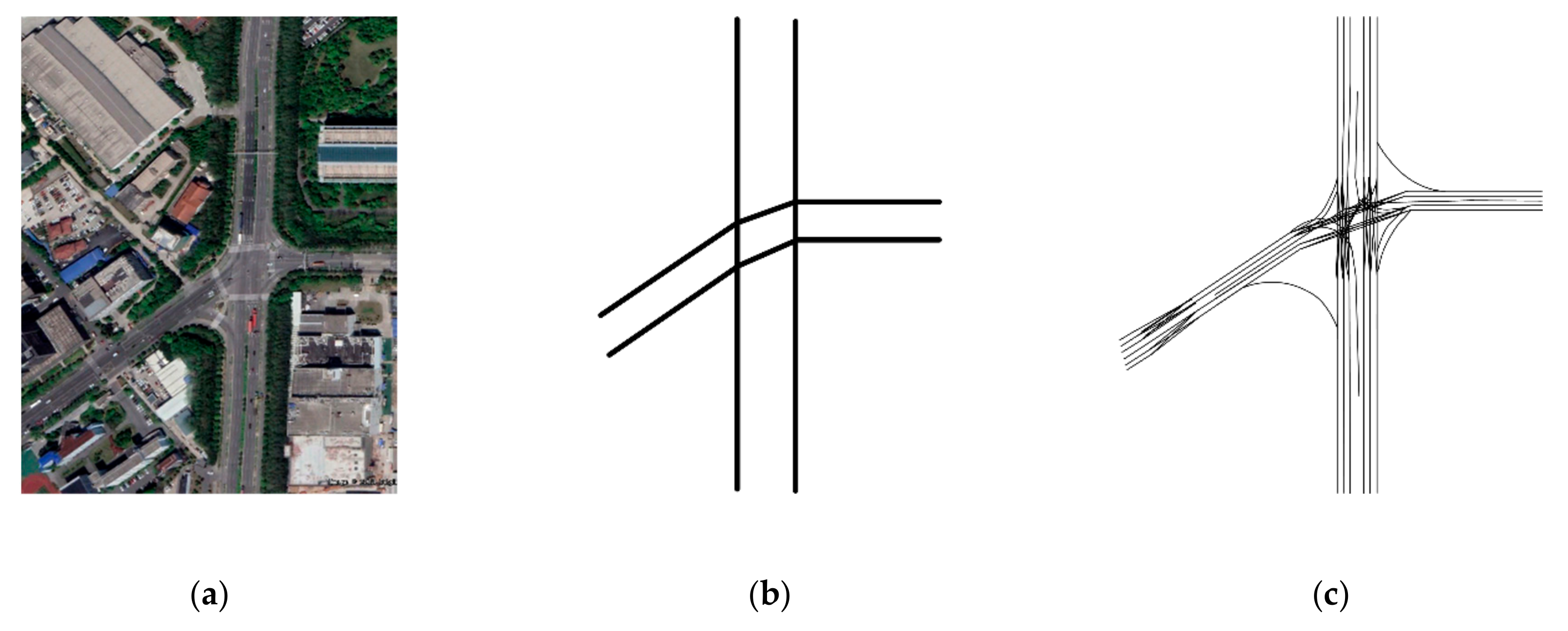
A lane-level map includes a lane-level road network, lane-level attribution in detail, and lane geometry lines with high accuracy, from the 10 cm level to the decimeter level modeling the real world. A road network describes the road system of the real world and a lane-level road network is a fundamental part of a lane-level map. Figure 1 shows examples of the road-level road network and lane-level road network representing the real world. There are various research studies on lane-level road networks in the literature, including different approaches to automatic lane-level road network generation, lane-level intersection extraction, and lane-level road network graph construction. However, there is a lack of summary and comparison of these works. This paper presents an overview of the sensors and the techniques for the generation of a land-level road network. First, we introduce the sensors for lane-level road network collection. Second, we discuss the lane-level road geometry extraction methods of a lane-level road network for autonomous driving. Third, we present the mathematical modeling and the logic representation of a lane-level road network. Finally, we provide a discussion and conclusions of this work.
2. Sensors
There are different kinds of on-board systems for lane-level road network collection, the sensors of which can be classified into two main categories: position sensors and perception sensors. The former includes the Global Navigation Satellite System (GNSS), Inertial Navigation System (INS), and Position and Orientation System (POS), and the latter includes lasers and cameras. The following sections describe these sensors in detail.
2.1. Position Sensors
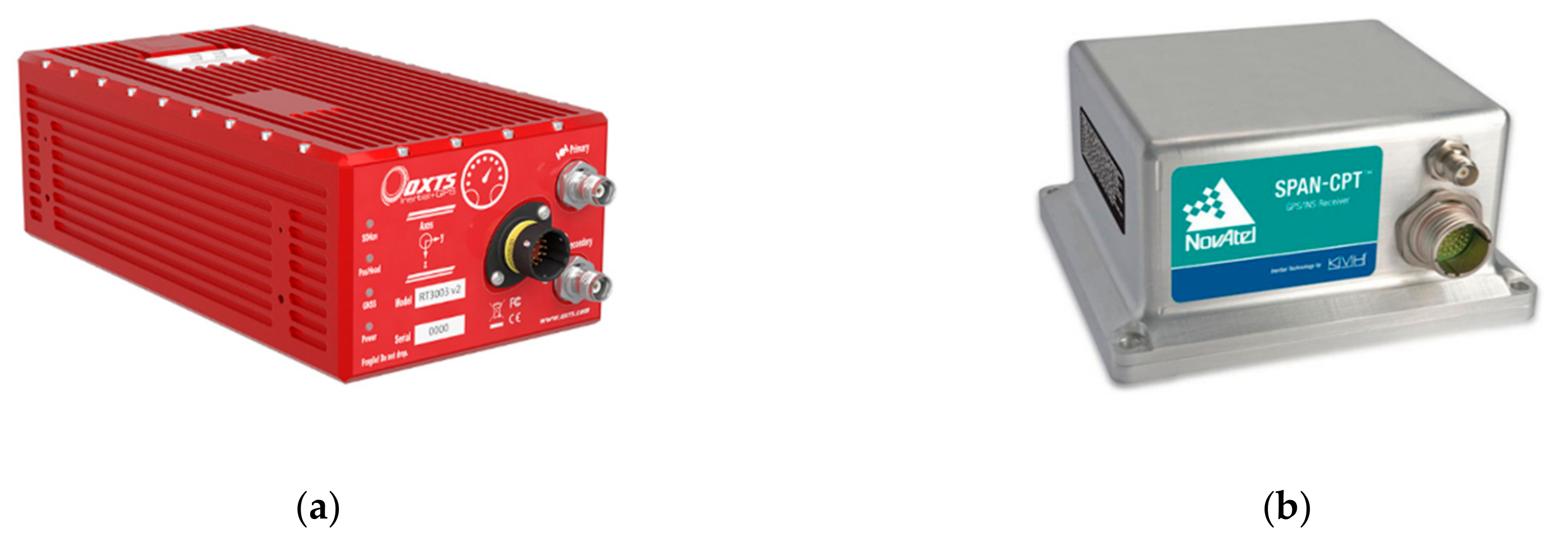
There are various modifications for an on-board collection system. The Global Navigation Satellite System (GNSS) usually utilizes Differential GPS (DGPS) technology for lane-level road network acquisition [29], which improves the position accuracy with real-time differential error data. GPS is a typical type of GNSS. Moreover, a crowdsourcing trajectory is sourced from crowd-sourced vehicles equipped with GPS and from GPS. In this approach, the sample frequency of the GPS is 5−120 s, and the average sample frequency is 5−60 s. Accordingly, the accuracy for samples is meters to tens of meters. For example, U-blox EVK-6T is low cost, and the position accuracy is 2.5 m [30]. In addition, the Inertial Navigation System (INS) provides the positions of vehicles with Inertial Measurement Units (IMU) with gyro and accelerometers. Furthermore, the Position and Orientation System (POS) combines the GNSS, the INS, and the Distance Measurement Instrument (DMI) to provide position and posture information, which can further enhance the performance of the INS by integration with differential GPS. This system has been adopted by a probe vehicle, which was equipped with other on-board sensors for lane-level road network collection. NovAtel SPAN-CPT (NovAtel Inc., Calgary, Canada) series devices have been used in preliminary studies. The data update frequency of this system is 100 Hz, and the position accuracy is at the centimeter level [31]. OXTS RT3000 (Oxford Technical Solutions Ltd., Oxfordshire, United Kingdom) has the same data update frequency and position accuracy [32]. In addition, the NovAtel SPAN FSAS, which can support the addition of a DMI SICK DFS60B, was designed with 200 Hz for raw data updates, whose absolute accuracies are 0.02 m for the spatial position, 0.08° for the pitch angle, 0.023° for the yaw angle, and 0.008° for the roll angle [28]. Figure 2 shows the sample images of OXTS RT3002 and NovAtel SPAN-CPT.
2.2. Perception Sensors
In addition to extracting position data directly, other studies have used perception sensors that combine position sensors for an on-board system. The perception sensors of an on-board system used to extract a lane-level road network can be divided into two categories: laser scanners and cameras. The subsequent sections describe these sensors in detail.
2.2.1. Laser Scanners
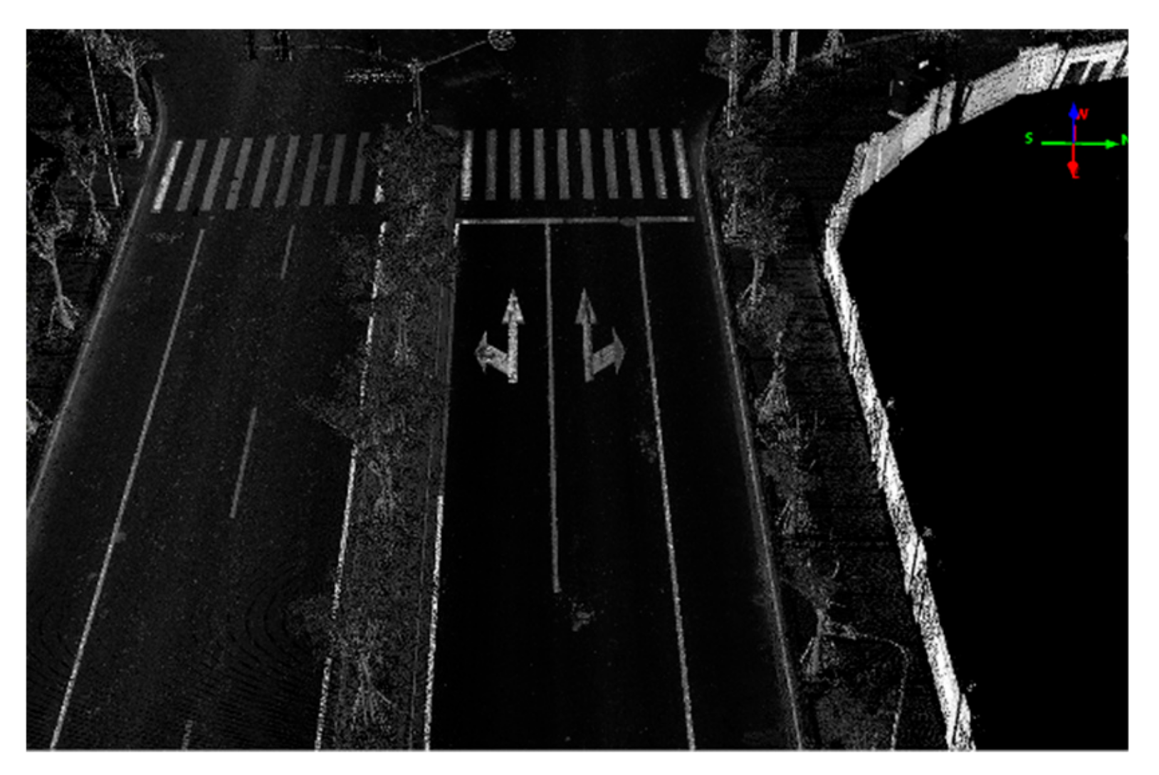
Laser scanners emit laser pulses to detect objects, which reflect signal light back to a laser pulse and calculate the position and velocity of objects with a reflected signal light. A laser scanner consists of the scanning system and ranging system, integrating charge-coupled device (CCD), the control system and calibration system. Original observation data of a laser scanner include time, distance, angle and reflected intensity, which further can calculate position and reflected intensity information. Additionally, the surface reflectivity of a scanned object depends on the surface color and the surface type such as smooth or rough, which could influence the ability of the laser scanner. The higher the reflectivity of the scanned object, the more light signals the scanned object can reflect and the longer the range of the laser scanner. Figure 3 shows an example of the reflected intensity image of a laser scanner.
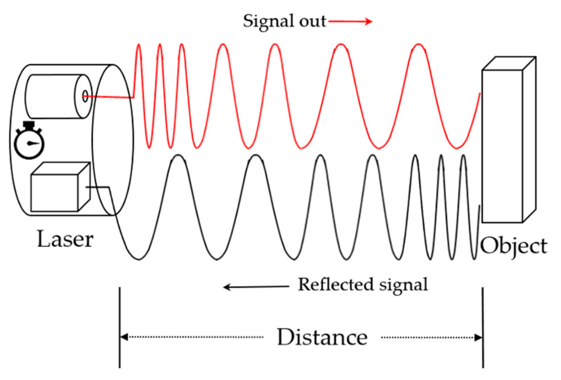
In previous study [33], the classification of lasers based on measurement principles includes five categories: time of flight (TOF) sensors, triangulation sensors, confocal sensor interferometric sensors, fiber Bragg grating sensors, and laser Doppler velocimetry, where a specific and detailed report of these categories have been described. Since most lasers used for the lane-level road network extraction of existing studies use TOF sensors, we take the TOF sensor as an example. Figure 4 shows the schematic diagram of a TOF. A TOF sensor emits and receives laser pulses, then it records the time interval between a pulse emission and return to calculate the distance between a scanner and objects. In this approach, the measuring distance range is several hundred meters, or even one kilometer. For example, a Velodyne HDL-32E sensor, which has a 360° horizontal and a 40° vertical field of view, is designed for less than 2 cm of measurement for distance accuracy and 70 m for distance. This sensor has been widely used on a probe vehicle for lane-level road network extraction [34,35]. The scanning frequency of this laser is 10 Hz, providing 700,000 points per second. In addition, the Velodyne HDL-64E is an improved laser, with 120 m in measurement distance and 1.333 million survey points [36]. Moreover, a RIEGL Vz-400 has been used for professional surveys such as the Mobile Mapping System (MMS) [37], which has a 360° horizontal and 100° vertical field of view. The scanning distance of this laser reaches 600 m for 90% reflectivity, and the accuracy is 3 mm. The emitting frequency is 1.2 million points per second.
2.2.2. Cameras
A digital camera sensor provides digital images where image information such as color, intensity, and texture can be used to detect objects in the scene. Since cameras are low-cost compared to other sensors such as laser scanners, it has been a research hotspot for lane extraction [38,39]. Sensors for vision-based studies include single cameras and stereo cameras [40]. Additionally, multi-cameras are used as vision sensors [41]. Although the theory of a monocular camera has made considerable progress in recent years, a monocular camera is limited in terms of the position and size extraction of objects due to the lack of depth information. Accordingly, stereo camera sensors have been adopted to recover depth information [42]. These camera sensors obtain spatial 3D information with two planar images shot from different perspectives. Fan and Dahnoun [43] improved the detection rate of lanes successfully using these sensors. Furthermore, multi-cameras consist of several cameras that provide complementary information and verification of information between cameras [39].
2.3. Summary
A single-position sensor can collect the lane-level road network data directly, but the sensor is expensive, while a multi GPS approach obtains lower accuracy for a lane-level road network but has a cheaper cost. Besides, crowdsourcing trajectory data updates rapidly. A laser scanner is appropriate for extracting the high precision of a lane-level road network, but it costs a large amount and it can be affected by bad weather such as snow or fog. A camera is cheap but sensitive to weather and light. Table 1 shows the results of the sensors comparison.
3. Lane-Level Road Geometry Extraction Methods
Lane-level road networks do not update in real time for lane-level maps of autonomous vehicles. The generation results of a lane-level road network are consistent whether using perception sensors or position sensors. Since perception sensors directly provide relative data, it is necessary to use data preprocessing and data registration in order to obtain absolute data. More comprehensive and detailed reports on the lane-level road network generation process from perception sensors can be found in previous studies [44,45], although this is not the key concern in this study. We focus on the road geometry extraction for a lane-level road network and divide lane-level road geometry extraction methods into three categories: trajectory-based methods, 3D point cloud-based methods, and vision-based methods. The following subsections address the methodology, advantages, and limitations for each category.
3.1. Trajectory-Based Methods
The trajectory-based methods focus on lane centerline extraction. The single GPS trajectory-based method regards the GPS trajectory as the lane centerline, and this trajectory is recorded by a probe vehicle driving along the centerline of a lane. This method models lane geometry directly, so it is widely used [28,46]. However, the accuracy of the lane geometry relies on the position accuracy of the probe vehicle. Research studies have focused on improving the accuracy and reliability of the probe vehicle position. In reference [7], the authors used GPS-combined Dead Reckoning (DR) to get a more accurate vehicle position. Additionally, their inertial and GPS measurements fusion method used a Bayesian filter, which improved the reliability of the probe vehicle position measurements [47,48].
Crowdsourced GPS trajectories are widely used for road-level information extraction [5,49,50,51], such as road geometry and topology extraction [52,53,54]. With adequate mining, the crowdsourcing trajectories have been another data source for lane-level road network extraction. Methods based on the crowdsourcing trajectories analyze the shape feature and direction feature of trajectories to mine the lane information in detail using massive GPS trajectories. In general, the extraction of lane geometry contains three steps. First, the noise of the raw trajectories is filtered. For example, previous studies have used a Kalman filter and a particle filter algorithm [55] or kernel density methods [49] for preprocessing. Second, the lane number of the segment is inferred. Third, the lane geometry is constructed using traffic rules. In previous study [56], the authors used nonparametric Kernel Density Estimation (KDE) to estimate the number and the locations of the lane centerlines. Tang et al. [57] proposed a naive Bayesian classification to extract the number and the rules of traffic lanes, and they achieved no more than 84% precision on the lane number extraction. In addition, an optimized constrained Gaussian mixture model was proposed in order to mine the number and locations of the traffic lanes, and the precision of the lane number was 85% [29]. The results revealed that there was still room to improve the accuracy and precision of the lane geometry [58], although the crowdsourcing trajectories method was economical.
3.2. 3D Point Cloud-Based Methods
Perception-based methods usually extract lane markings to get the lane geometry (such as lane lines and arrows), since lane markings reflect the high intensity values on the road surface. Accordingly, the methods of previous studies have been mainly divided into two categories: point-cloud-based methods and georeferenced feature (GRF) vision-based methods. A more detailed introduction to perception-based methods can be found in previous study [44].
3.2.1. Point-Cloud-Based Methods
Point-cloud-based methods are the most commonly and directly adopted methods used to extract lane markings. Since the characteristics of the high retro reflectivity and intensity of point clouds are different from road surfaces, single-threshold methods have been developed to extract road markings, for which a global threshold parameter has been implemented for all the point cloud scenes. In previous study [59], the authors detected lane markings for a certain threshold successfully according to their strength of reflection. The authors in previous study [32] used a simple single-intensity threshold to extract points whose intensities were greater than a threshold. However, single-threshold methods may achieve misleading extraction results because of the inconsistent point clouds in the real world. Accordingly, multi-threshold methods have been studied to improve extraction of points with inconsistent strength [60]. Otsu’s thresholding approach [61] was used to provide optimal threshold parameters that adjusted different point distributions for several scenes of point clouds [62]. The authors in previous study [63] adopted a gradient value as a multi-threshold to extract lane markings successfully. In previous study [64], with the use of multi-threshold methods, the precision of the lane marking points was 90.80%. With these methods, point clouds need to segment and block, with sizes being uncertain. Moreover, threshold methods do not work well on a non-obvious intensity contrast between lane markings and road-surface surroundings, which can easily lead to leakage and fault extraction. In addition, many studies have used Convolutional Neural Networks (CNN) to automatically classify road markings [65,66]. In previous study [65], a conditional generative adversarial network (cGAN) was used for small-size road marking classification, and the precision was no more than 96%. However, CNN methods require manual work on the class label of a training set, which limits its wide use on a large region.
3.2.2. GRF Vision-Based Methods
Another approach to processing point clouds is to convert point clouds into a georeferenced feature image and extract the schematic of the image. The studies on georeferenced vision-based methods have included Hough Transforms, multiscale threshold segmentation, and multiscale tensor voting (MSTV) methods. A Hough Transform is commonly used in line identification. In previous study [59], a Hough Transform based on the strength of a reflection was applied in the generated GRF image. However, the Hough Transform does not adapt well to complex conditions. Accordingly, multiscale threshold segmentation methods were implemented to automate the extraction of various types of road markings that combined both the distribution of the intensity values and the ranges of scanning [67]. For instance, lane markings were successfully extracted by a trajectory-based multisegment thresholding method in previous study [62]. In addition, the authors in [68] applied a range-dependent thresholding method for extraction from surface point clouds, while the authors in [69] used a point-density-dependent multi-threshold segmentation method to segment georeferenced images. Moreover, the road marking precision was no more than 95% with the multisegment thresholding method used in previous study [70]. In addition, an MSTV method was used in order to improve the extraction of a noisy GRF image. For instance, the authors in previous study [71] used MSTV to extract the crack pixels of a GRF image, which were segmented by a modified inverse distance-weighted method based on point density.
3.3. Vision-Based Methods
The construction of a lane-level road network relies on vision-based methods, which generally extract the lane lines of road geometry combined with GPS data. Vision-based methods for lane extraction have become a hot topic [72,73,74] in recent decades because of the low cost of vision equipment. These methods are mainly categorized into two types: feature-based and model-based methods [75]. Feature-based methods rely on several features of lane lines, such as color, gradient, line width, and edges. A Sobel detector and a Canny detector are commonly applied in the edge detection of lane lines. Using a gradient, the authors in previous study [76] made full use of directional and shape features to extract lane lines. However, feature-based methods are sensitive to image noise and environmental conditions such as shade or varying light, while model-based methods perform well in these conditions. Model-based methods focus on the structure of a lane. To establish the mathematical model of a structure, a Hough transform [77] was used in the pre-extraction before curve fitting. A Hough transform and a shape-preserving spline fitted the lane smoothly [78]. In previous study [79], the authors combined a Hough transform and a least-squares line-fitting model, while authors in previous study [80] combined a Hough Transform and a Gaussian mixture model in the processing of lane detection. Moreover, a Random Sample Consensus (RANSAC) [43,81,82] fitting method was used to calculate the lane model parameters in preliminary studies. For example, the authors in [83] used inverse perspective mapping (IPM) to transform image and RANSAC parabola fitting to detect lane markings. However, model-based methods have not been adapted to various scenarios.
In order to improve the performance of lane extraction in complex conditions, CNN based on deep learning was implemented. In previous study [84], the authors proposed a multi-task deep convolutional method to detect lane markings and geometry. A you only look once (YOLO) v3 algorithm was applied to lane extraction in complex lane conditions [85]. A Vanishing Point Guided Network (VPGNet) was studied to solve the extraction of lanes under complex weather conditions [83]. A Mask R-CNN reached 97.9% accuracy on TSD-Max datasets [86]. Time consumption is still a challenge for CNN-based extraction.
3.4. Summary
Chapters in this section review lane-level road geometry extraction methods, and it is divided into three parts based on different data sources for the methods. The trajectories-based methods extract centerlines to generate lane-level road networks, while 3D point-cloud-based methods and vision-based methods mainly extract the boundaries of lanes for lane-level road network generation. In addition, 3D point-cloud-based methods are more accurate and costly compared to vision-based methods. Moreover, each method category has advantages and disadvantages. Table 2 presents a comparison of lane-level road geometry extraction methods.
4. Mathematical Modeling of Lane-Level Road Network
When the geometry of a lane has been extracted, it is essential to model the lane-level road network for direct use by autonomous driving applications. The mathematical modeling of a lane-level road network includes lane mathematical modeling and intersection mathematical modeling. We will discuss these types of modeling in this section, and the latter type of modeling is key content that will be described in detail.
4.1. Lane Mathematical Modeling
Mathematical models of a lane-segment are consistent with mathematical models of a road-segment, for which a large number of achievements and summaries have been produced in past studies [87,88,89,90]. For this paper, we do not discuss these mathematical models in detail. These mathematical models include straight line, arc curves, Clothoid curves, several spline curves and polylines.
4.2. Intersection Mathematical Modeling
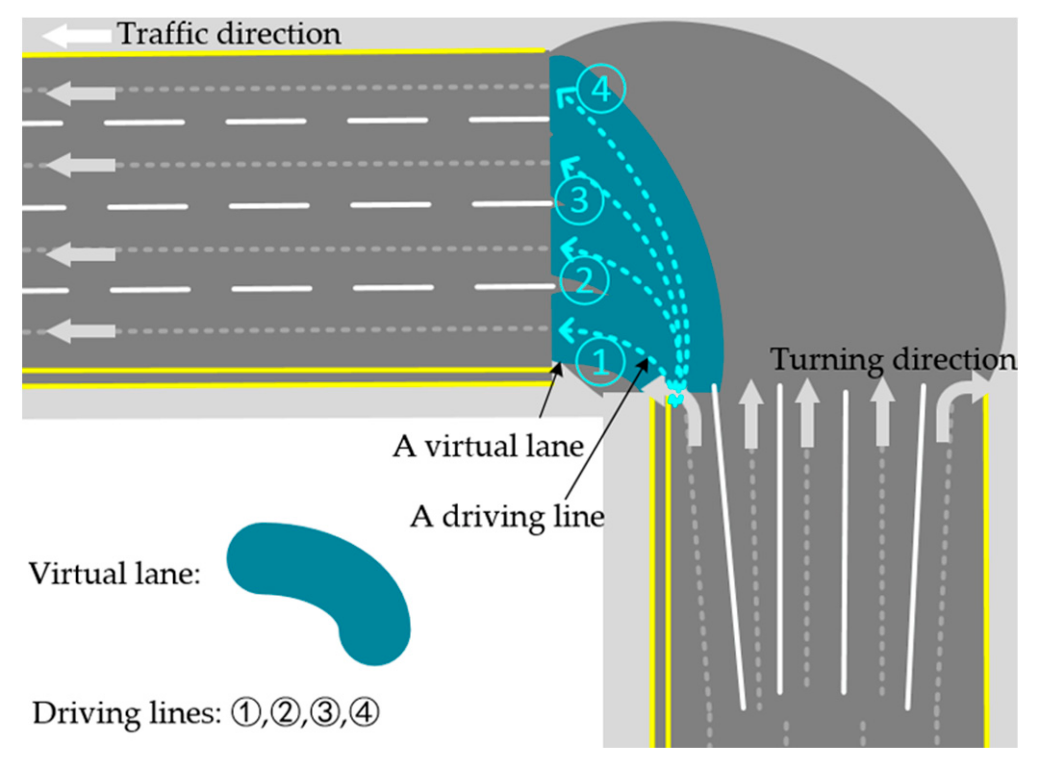
When the geometry of a lane has been extracted, it is easy to obtain an intersection and it is essential to represent the intersection in detail. An intersection of a lane-level road network includes not only the zone of the intersection but also the topological relationship with traffic rules. Virtual lanes are widely used for autonomous driving navigation in an intersection [45]. Driving lines can be used to abstractly represent virtual lanes with both the information of a path and regular turning traffic [70]. There are several mathematical functions for modeling driving lines, including arc curves, spine curves, and polylines. The subsequent sections describe these mathematical modeling functions in detail. Figure 5 shows an example of the virtual lanes and driving lines of one turning direction in an intersection.
4.2.1. Arc Curves
An arc curve is composed of arcs and line segments. It is uniquely defined by three different points, and a smooth curve does not allow self-intersection. Curvature is a step function and the tangent line unit vectors are equal at the breakpoints given by the two corresponding segments. Arc curves have constant characteristics such as rotation, translation, and scaling. Since it is represented in a closed form, the offset curve of a circular spline is actually a circular spline that provides accurate offset and arc length calculations, as well as the calculated distance from the closest point to the curve. It is especially simple to compute the distance from a point to a curve. In addition, the arc curves are compatible with all established geometries and Computer-Aided Design (CAD) systems for practical applications. Compared to Clothoids or polylines, arc splines can be represented in the form of parameterless descriptions, and visualization calculations are much more efficient [17]. Authors in previous studies [91,92] adopted an arc curve to generate the driving line of an intersection, and it performed well in fitting, particularly at circular intersections (such as roundabouts).
4.2.2. Cubic Spline Curves
A B-spline is a spline composed of control points, node vectors, and primary functions. The shape of a B-spline curve can be changed by modifying one or more of these control parameters. Given n + 1 points {} and m + 1 node vectors {}, the node vector is the polynomial with the highest degree k and and; the B spline can be expressed by Formula (1), and is the primary function.
B-spline representation of road geometry is widely used in road modeling [93,94]. In addition, a B-spline curve has the advantages of a convex shape, local correction of control points, and numerical stability, which are used to approximate the shape of the road. In previous study [90], the authors proposed a progressive correction algorithm to reduce the number of control parameters in the B-spline curve to accurately represent the lane geometry. Based on this research, the authors in previous study [95] proposed an adaptive curve refinement method based on a dominant point that used a B-spline mathematical curve model to describe the 3D road geometry information, which took into account the road shape factors (the curvature, arc, etc.). This method reduced the number of nodes and control points of the B-spline road model while ensuring the accuracy of the road network.
A cubic Hermite spline (CHS) is another type of cubic spline curve that is linearly parameterized [96]. A CHS with two nodes is generally used. Given two nodes, the corresponding function values are and the corresponding derivative values are. Then, the cubic Hermite polynomial between two points is as shown in Formula (3):
A CHS has the following characteristics: First, there is a C1 continuity between the control points in each CHS segment. Second, the CHS curve representation has global C2 continuity between adjacent control points at the series point, since the point between the cascaded CHS segments, the interconnection point, and the tangent are the same. Third, the parameters indicated by the CHS are the position and the tangent of the control points, and a series of point features can be used to parameterize any lane curve. These vertex attributes are compatible with the data structures of common GIS database software. Fourth, the accuracy of the CHS lane representation can be manipulated by increasing or decreasing the CHS control point (i.e., increasing or decreasing the vertices) so that the CHS can extract the lane parameters through local control. A Catmull–Rom spline is a subclass of a CHS that has been successfully used to model the transition driving lane [45].
4.2.3. Polylines
Piecewise polynomial functions can be used to represent polylines, which refer to dividing continuous space into m + 1 segments with m segment points, where each of the segments can be represented by a separate polynomial primary function. It is assumed that the continuous definition domain X is a one-dimensional vector, and segment points divide the definition domain X of into continuous space with a primary function of . Then the piecewise polynomial function can be expressed by Formula (3):
Since it is convenient to use polynomials to calculate a derivative, important information such as tangent angle and curvature can be extracted from a fitted spline curve by simple arithmetic operations [97]. In order to intuitively describe and reduce computational complexity, a cubic polynomial is usually segmented to fit a curve segment. However, due to the differences in intersections, it is difficult to approximate intersections with a set of piecewise polynomials. This process usually requires more segmentation polynomials and results in computational complexity. The authors in previous study [32] proposed an effective curve approximation algorithm based on polylines that used the smallest number of piecewise polynomials to represent the lane, including the intersection, and the computational complexity was. This algorithm solved the problem of the piecewise polynomial fitting in a large-scale road network.
4.3. Summary
The mathematical model used to abstractly represent a drive line in an intersection corresponds to the use for the representation of a lane or an abstracted segment of a road. In mathematical functions, arc lines have been widely used for circle intersections because they require less computation compared to other curves. Other curves exhibit flexibility in modeling irregular intersections, but they have the problem of finding a proper control point or an optimal optimization.
5. Lane-Level Road Network Logic Representation of Classic Lane-Level Map Formats
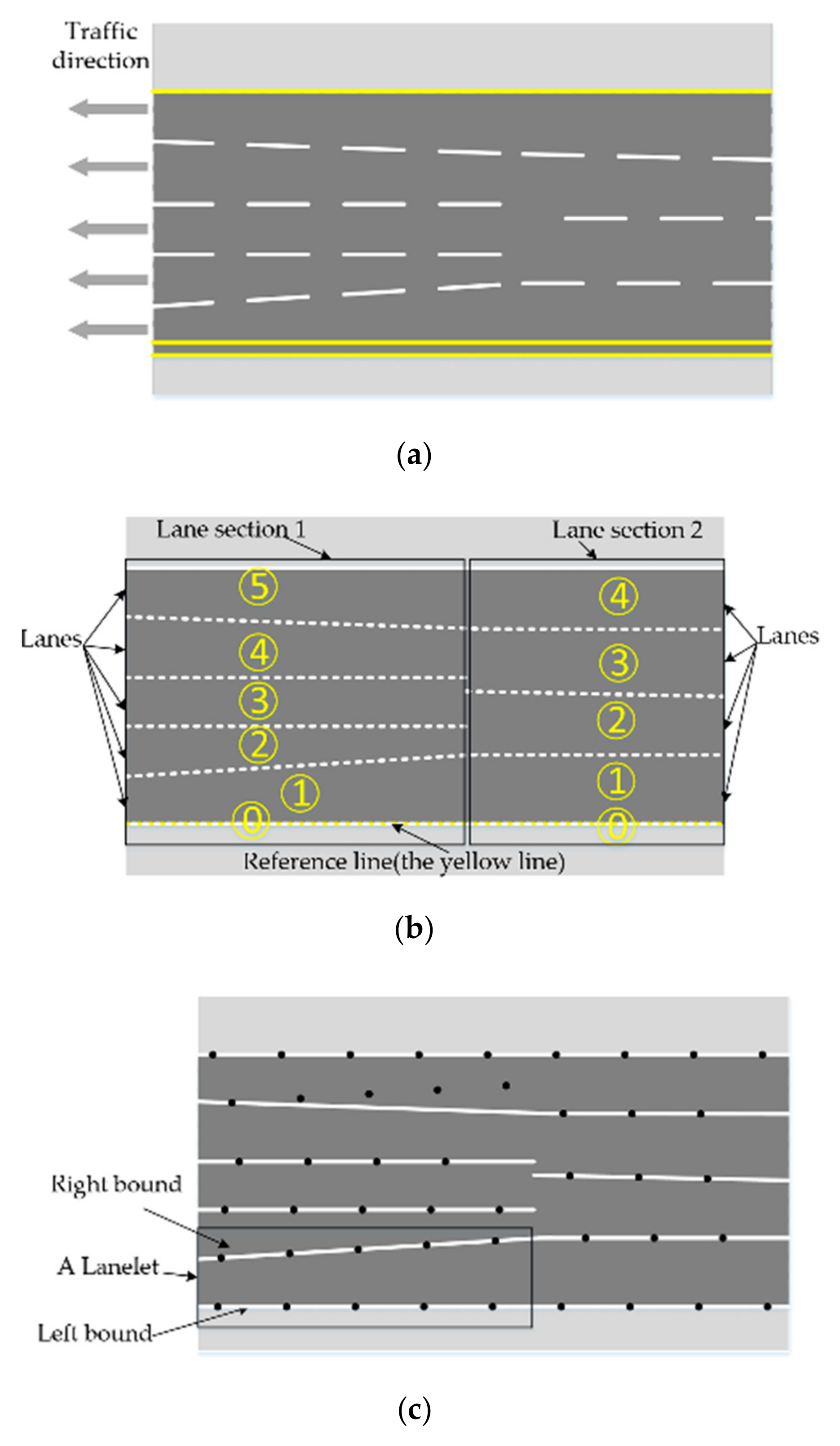
In recent years, there have been several classic lane-level map formats that have been developed with applications in autonomous driving applications. Classic lane-level road network representations are consistent with respect to lane information, but different with respect to the logic representation. Since a lane-level road network is an important part of a lane-level map, the logic formats of lane-level road networks vary with the various formats of lane-level maps. Moreover, to meet the increasing requirements of autonomous driving applications, the logic representations of lane-level road networks have not formed uniform formats or regulations, and they develop and update rapidly with the rapid development of autonomous driving technology. However, different lane-level road network formats contain complete lane-detail information (such as lane width, curve, slope, etc.) and the logic representations can create interconversion, although not all conversions of lane-level road network formats have been published [98]. To summarize, a detailed description of the lane information is added in a lane-level road network. Based on previous studies, we divided the formats into two categories based on the models of the geometry and the topology of the lanes: The node-arc-based model and the segment-based model. Figure 6 shows examples of the logic representation of a lane based on different models.
The node-arc model is the model which is generally used in road-level road networks, where segments of roads are abstracted by road centerlines and further represented by nodes and arcs. In a lane-level road network, lane centerline model lanes consist of nodes and arcs, and the properties of the lane are described by the attributes of the arcs or nodes. Additionally, the topology relationships of lanes are represented by the link relationships of node-to-node, node-to-arc, or arc-to-arc. A Route Network Definition File (RNDF) was first proposed on the 2007 DARPA urban challenge [99]. For the basic structure of an RNDF, segments are composed of one or more than one lane, while lanes are composed of one or more than one waypoint. The Navigation Data Standard (NDS) released the Open Lane Model (OLM) [100], which proposed a high accuracy of more than 1 cm for the topology structure and geometry of a lane. The connection model of the complex intersection was made with arcs and points. Since it is a commercial format, the detail of this model was not open to the public. In previous study [101], the authors proposed a seven-layer lane-level map model based on a traditional road-level navigation electronic map by adding a lane layer. In this model, a lane was abstracted by the centerline of the lane. In summary, the key basic structure of a line in a node-arc model cannot precisely represent the shape of a lane, which is usually the additional attribution; however, this is very advantageous for route planning and route searching.
The segment-based model uses the segment of the lane to abstract the lane instead of the shape of a line or arc. The segment consists of the zone covered by a lane and the left and right bound of a lane. Nonetheless, the representation of a lane bound may be a point or a polyline. For example, OpenDrive set the reference line of a road to define the basic geometry. Lanes were divided into lane sections along the road based on the attribution changes of a road and they were numbered by the offset of the line [102]. In this format, the lane bounds are consisted of points. In addition, Bender, Ziegler, and Stiller [21] proposed lanelets. In this format, a lanelet is an atomic lane segment that is characterized by the left and right lane bounds. Road segments are abstracted by lanelets and the adjacent lanelets are used to represent the topological relationship between lanes. The lane boundary line of a lanelet is abstracted by a polyline. Based on the lanelet, lanelet2 revised the map structure and developed a software framework available for the public [103]. Additionally, the format of OpenDrive can convert to the format of lanelet2 [98]. To summarize, the segment model describes the precise shape of a lane. However, it cannot directly support global route planning before extra work is done. Figure 7 shows examples of a lane representation by OpenDrive and lanelets.
Generally, the two types of lanes provide detailed and precise lane information such as lane boundaries and curves, which is essential for autonomous driving. However, lane-level road networks for autonomous driving are still in the early stages, and there are many challenges to overcome for the testing and updating of a large lane-level road network.
6. Discussion and Conclusions
6.1. Synthesis of Findings
Nowadays, autonomous driving is a hot topic and there have been several hundreds of autonomous vehicles in China. A lane-level map is of fundamental importance to autonomous driving with regard to sensing and perception, planning, and control. A road network describes the road system of the real world and a lane-level road network is a fundamental part of a lane-level map. Such lane-level road network data are used not only for intelligent driving, but also for cooperative vehicle infrastructure systems and intelligent cities. In past years, maps have been developed for autonomous driving and several sensors have been used to collect lane-level road network data. However, there is still room for improvement in the data collection and the production of the lane-level road network. In addition, lane-level maps have not reached a consensus state and neither have the formats of lane-level road networks. The development of lane-level maps is rapidly evolving with the development of autonomous driving. In a word, lane-level road networks for autonomous driving are still in the early stages. Moreover, in order to sufficiently meet the demands of autonomous driving applications, a lane-level road network must contain lane information in detail. However, there is not a sufficient number of studies on evaluation index of the road network for lane-level maps of autonomous vehicles. Further research must be carried out in this field.
In this paper, we reviewed lane-level road network generation techniques for the lane-level maps of autonomous vehicles with on-board systems based on the generation and the representation of lane-level road networks. For the generation of lane-level road networks, the paper was structured in two sections: sensors and lane-level road geometry extraction methods. Based on the studies, each category of sensors had advantages and disadvantages for different on-board systems. They were all the available data sources for lane-level road network collection. The extraction methods were further divided into three categories: trajectory-based methods, 3D point-cloud-based methods, and vision-based methods. Point-cloud-based methods were the highest accuracy approaches, vision-based methods were the most economical, and trajectory-based methods were direct approaches for constructing centerline lane-level road networks. For the representation of lane-level road networks, we introduced mathematical modeling and logic formats. Based on the studies, the mathematical modeling of a lane-level road network included lane mathematical modeling and intersection mathematical modeling. For the analysis of the literature of driving line models of intersections, an arc curve was simplest and fit well for the condition of a roundabout intersection, while other curves were more adaptive for irregular intersections. Finally, although the classic formats varied in the structure of lane representation, all formats included complete lane information.
6.2. Future Research Avenues
Since widespread applications of autonomous driving technology accelerate the development and commercialization of the lane-level map, new requirements of data capacity, accurate degree, and update frequency of the lane-level road network have been put forward. Moreover, the application of artificial intelligence technology in lane-level road network extraction can change the processing of the collection and production of the lane-level road network. In addition, based on the technology of Internet of Things and fifth-generation wireless communication, edge computing provides a new data-processing model for the lane-level road network based on crowdsourcing.
Author Contributions
This research was carried out by the co-authors. Conceptualization, B.L. and L.Z.; writing, L.Z.; investigation, B.Y., H.S., and Z.L.
Funding
This research was funded by the National Natural Science Foundation of China (Grant Numbers. 41671441, 41531177, and U1764262).
Conflicts of Interest
The authors declare no conflict of interest.
References
- Fraedrich, E.; Heinrichs, D.; Bahamonde-Birke, F.J.; Cyganski, R. Autonomous driving, the built environment and policy implications. Transp. Res. Part A Policy Pract. 2019, 122, 162–172. [Google Scholar] [CrossRef] [Green Version]
- Xu, X.; Fan, C.-K. Autonomous vehicles, risk perceptions and insurance demand: An individual survey in China. Transp. Res. Part A Policy Pract. 2018, 124, 549–556. [Google Scholar] [CrossRef]
- Ji, J.; Khajepour, A.; Melek, W.W.; Huang, Y. Path planning and tracking for vehicle collision avoidance based on model predictive control with multiconstraints. IEEE Trans. Veh. Technol. 2016, 66, 952–964. [Google Scholar] [CrossRef]
- Chen, Z.; Yan, Y.; Ellis, T. Lane detection by trajectory clustering in urban environments. In Proceedings of the 17th International IEEE Conference on Intelligent Transportation Systems (ITSC), Qingdao, China, 8–11 October 2014; pp. 3076–3081. [Google Scholar]
- Ahmed, M.; Karagiorgou, S.; Pfoser, D.; Wenk, C. A comparison and evaluation of map construction algorithms using vehicle tracking data. GeoInformatica 2015, 19, 601–632. [Google Scholar] [CrossRef]
- Nedevschi, S.; Popescu, V.; Danescu, R.; Marita, T.; Oniga, F. Accurate Ego-Vehicle Global Localization at Intersections Through Alignment of Visual Data With Digital Map. IEEE Trans. Intell. Transp. Syst. 2013, 14, 673–687. [Google Scholar] [CrossRef]
- Bétaille, D.; Toledo-Moreo, R. Creating enhanced maps for lane-level vehicle navigation. IEEE Trans. Intell. Transp. Syst. 2010, 11, 786–798. [Google Scholar] [CrossRef]
- Rohani, M.; Gingras, D.; Gruyer, D. A Novel Approach for Improved Vehicular Positioning Using Cooperative Map Matching and Dynamic Base Station DGPS Concept. IEEE Trans. Intell. Transp. Syst. 2016, 17, 230–239. [Google Scholar] [CrossRef]
- Driankov, D.; Saffiotti, A. Fuzzy Logic Techniques for Autonomous Vehicle Navigation; Physica-Verlag GmbH: Heidelberg, Germany, 2013; Volume 61. [Google Scholar]
- Cao, G.; Damerow, F.; Flade, B.; Helmling, M.; Eggert, J. Camera to map alignment for accurate low-cost lane-level scene interpretation. In Proceedings of the Intelligent Transportation Systems (ITSC), IEEE 19th International Conference, Rio de Janeiro, Brazil, 1–4 November 2016; pp. 498–504. [Google Scholar]
- Gruyer, D.; Belaroussi, R.; Revilloud, M. Accurate lateral positioning from map data and road marking detection. Expert Syst. App. 2016, 43, 1–8. [Google Scholar] [CrossRef]
- Suganuma, N.; Uozumi, T. Precise position estimation of autonomous vehicle based on map-matching. In Proceedings of the Intelligent Vehicles Symposium, Baden-Baden, Germany, 5–9 June 2011; pp. 296–301. [Google Scholar]
- Aeberhard, M.; Rauch, S.; Bahram, M.; Tanzmeister, G.; Thomas, J.; Pilat, Y.; Homm, F.; Huber, W.; Kaempchen, N. Experience, results and lessons learned from automated driving on Germany’s highways. IEEE Intell. Transp. Syst. Mag. 2015, 7, 42–57. [Google Scholar] [CrossRef]
- Toledo-Moreo, R.; Betaille, D.; Peyret, F.; Laneurit, J. Fusing GNSS, Dead-Reckoning, and Enhanced Maps for Road Vehicle Lane-Level Navigation. IEEE J. Sel. Top. Signal Process. 2009, 3, 798–809. [Google Scholar] [CrossRef]
- Li, H.; Nashashibi, F.; Toulminet, G. Localization for intelligent vehicle by fusing mono-camera, low-cost GPS and map data. In Proceedings of the International IEEE Conference on Intelligent Transportation Systems, Funchal, Portugal, 19–22 September 2010; pp. 1657–1662. [Google Scholar]
- Tang, B.; Khokhar, S.; Gupta, R. Turn prediction at generalized intersections. In Proceedings of the Intelligent Vehicles Symposium (IV), Seoul, South Korea, 28 June–1 July 2015; pp. 1399–1404. [Google Scholar]
- Kim, J.; Jo, K.; Chu, K.; Sunwoo, M. Road-model-based and graph-structure-based hierarchical path-planning approach for autonomous vehicles. Proc. Inst. Mech. Eng. K-J. Mul. 2014, 228, 909–928. [Google Scholar] [CrossRef]
- Lozano-Perez, T. Autonomous Robot Vehicles; Springer-Verlag: New York, NY, USA, 2012. [Google Scholar]
- Liu, L.; Wu, T.; Fang, Y.; Hu, T.; Song, J. A smart map representation for autonomous vehicle navigation. In Proceedings of the 2015 12th International Conference on Fuzzy Systems and Knowledge Discovery (FSKD), Zhangjiajie, China, 15–17 August 2015; pp. 2308–2313. [Google Scholar]
- Shim, I.; Choi, J.; Shin, S.; Oh, T.-H.; Lee, U.; Ahn, B.; Choi, D.-G.; Shim, D.H.; Kweon, I.-S. An autonomous driving system for unknown environments using a unified map. IEEE Trans. Intell. Transp. Syst. 2015, 16, 1999–2013. [Google Scholar] [CrossRef]
- Bender, P.; Ziegler, J.; Stiller, C. Lanelets: Efficient map representation for autonomous driving. In Proceedings of the 2014 IEEE Intelligent Vehicles Symposium Proceedings, Dearborn, MI, USA, 8–11 June 2014; pp. 420–425. [Google Scholar]
- Jetlund, K.; Onstein, E.; Huang, L. Information Exchange between GIS and Geospatial ITS Databases Based on a Generic Model. ISPRS Int. Geo-Inf. 2019, 8, 141. [Google Scholar] [CrossRef]
- Kuutti, S.; Fallah, S.; Katsaros, K.; Dianati, M.; Mccullough, F.; Mouzakitis, A. A survey of the state-of-the-art localization techniques and their potentials for autonomous vehicle applications. IEEE Internet Things J. 2018, 5, 829–846. [Google Scholar] [CrossRef]
- Chu, H.; Guo, L.; Gao, B.; Chen, H.; Bian, N.; Zhou, J. Predictive Cruise Control Using High-Definition Map and Real Vehicle Implementation. IEEE Trans. Veh. Technol. 2018, 67, 11377–11389. [Google Scholar] [CrossRef]
- Liu, C.; Jiang, K.; Yang, D.; Xiao, Z. Design of a multi-layer lane-level map for vehicle route planning. In Proceedings of the MATEC Web of Conferences, Hong Kong, China, 1–3 July 2017; p. 03001. [Google Scholar]
- Liu, J.; Xiao, J.; Cao, H.; Deng, J. The Status and Challenges of High Precision Map for Automated Driving. In Proceedings of the China Satellite Navigation Conference 2019, Beijing, China, 22–25 May 2019; pp. 266–276. [Google Scholar]
- Schröder, E.; Braun, S.; Mählisch, M.; Vitay, J.; Hamker, F. Feature Map Transformation for Multi-sensor Fusion in Object Detection Networks for Autonomous Driving. In Proceedings of the Science and Information Conference, Hefei, China, 21–22 September 2019; pp. 118–131. [Google Scholar]
- Zheng, L.; Li, B.; Zhang, H.; Shan, Y.; Zhou, J. A High-Definition Road-Network Model for Self-Driving Vehicles. ISPRS Int. Geo-Inf. 2018, 7, 417. [Google Scholar] [CrossRef]
- Tang, L.; Yang, X.; Dong, Z.; Li, Q. CLRIC: collecting lane-based road information via crowdsourcing. IEEE Trans. Intell. Transp. Syst. 2016, 17, 2552–2562. [Google Scholar] [CrossRef]
- Kim, C.; Cho, S.; Sunwoo, M.; Jo, K. Crowd-Sourced Mapping of New Feature Layer for High-Definition Map. Sensors 2018, 18, 4172. [Google Scholar] [CrossRef] [PubMed]
- Kaartinen, H.; Hyyppä, J.; Kukko, A.; Jaakkola, A.; Hyyppä, H. Benchmarking the performance of mobile laser scanning systems using a permanent test field. Sensors 2012, 12, 12814–12835. [Google Scholar] [CrossRef]
- Gwon, G.P.; Hur, W.S.; Kim, S.W.; Seo, S.W. Generation of a Precise and Efficient Lane-Level Road Map for Intelligent Vehicle Systems. IEEE Trans. Veh. Technol. 2017, 66, 4517–4533. [Google Scholar] [CrossRef]
- Suh, Y.S. Laser Sensors for Displacement, Distance and Position. Sensors 2019, 19, 1924. [Google Scholar] [CrossRef] [PubMed]
- Zhang, Y.; Wang, J.; Wang, X.; Li, C.; Wang, L. 3d lidar-based intersection recognition and road boundary detection method for unmanned ground vehicle. In Proceedings of the 2015 IEEE 18th International Conference on Intelligent Transportation Systems, Las Palmas, Spain, 15–18 September 2015; pp. 499–504. [Google Scholar]
- Li, K.; Shao, J.; Guo, D. A multi-feature search window method for road boundary detection based on LIDAR data. Sensors 2019, 19, 1551. [Google Scholar] [CrossRef]
- Joshi, A.; James, M.R. Generation of accurate lane-level maps from coarse prior maps and lidar. IEEE Intell. Transp. Syst. Mag. 2015, 7, 19–29. [Google Scholar] [CrossRef]
- Lemmens, M. Terrestrial laser scanning. In Geo-information; Springer: New York, NY, USA, 2011; pp. 101–121. [Google Scholar]
- Gupta, A.; Choudhary, A. A Framework for Camera-Based Real-Time Lane and Road Surface Marking Detection and Recognition. IEEE Trans. Intell. Veh. 2018, 3, 476–485. [Google Scholar] [CrossRef]
- Häne, C.; Heng, L.; Lee, G.H.; Fraundorfer, F.; Furgale, P.; Sattler, T.; Pollefeys, M. 3D Visual Perception for Self-Driving Cars Using A Multi-Camera System: Calibration, Mapping, Localization, and Obstacle Detection. Image Vision Comput. 2017, 68, 14–27. [Google Scholar] [CrossRef]
- Antony, J.J.; Suchetha, M. Vision Based vehicle detection: A literature review. Int. J. App. Eng. Res. 2016, 11, 3128–3133. [Google Scholar]
- Ji, X.; Zhang, G.; Chen, X.; Guo, Q. Multi-perspective tracking for intelligent vehicle. IEEE Trans. Intell. Transp. Syst. 2018, 19, 518–529. [Google Scholar] [CrossRef]
- Su, Y.; Zhang, Y.; Lu, T.; Yang, J.; Kong, H. Vanishing point constrained lane detection with a stereo camera. IEEE Trans. Intell. Transp. Syst. 2017, 19, 2739–2744. [Google Scholar] [CrossRef]
- Fan, R.; Dahnoun, N. Real-time stereo vision-based lane detection system. Meas. Sci. Technol. 2018, 29, 074005. [Google Scholar] [CrossRef] [Green Version]
- Ma, L.; Li, Y.; Li, J.; Wang, C.; Wang, R.; Chapman, M. Mobile laser scanned point-clouds for road object detection and extraction: A review. Remote Sens. 2018, 10, 1531. [Google Scholar] [CrossRef]
- Guo, C.; Kidono, K.; Meguro, J.; Kojima, Y.; Ogawa, M.; Naito, T. A Low-Cost Solution for Automatic Lane-Level Map Generation Using Conventional In-Car Sensors. IEEE Trans. Intell. Transp. Syst. 2016, 17, 2355–2366. [Google Scholar] [CrossRef]
- Zhang, T.; Arrigoni, S.; Garozzo, M.; Yang, D.; Cheli, F. A Lane-Level Road Network Model with Global Continuity. Transp. Res. Part C Emerg. Technol. 2016, 71, 32–50. [Google Scholar] [CrossRef]
- Toledo-Moreo, R.; Bétaille, D.; Peyret, F. Lane-level integrity provision for navigation and map matching with GNSS, dead reckoning, and enhanced maps. IEEE Trans. Intell. Transp. Syst. 2009, 11, 100–112. [Google Scholar] [CrossRef]
- Betaille, D.; Toledo-Moreo, R.; Laneurit, J. Making an enhanced map for lane location based services. In Proceedings of the 2008 11th International IEEE Conference on Intelligent Transportation Systems, Beijing, China, 12–15 October 2008; pp. 711–716. [Google Scholar]
- Wang, J.; Rui, X.; Song, X.; Tan, X.; Wang, C.; Raghavan, V. A novel approach for generating routable road maps from vehicle GPS traces. Int. J. Geogr. Inf. Sci. 2015, 29, 69–91. [Google Scholar] [CrossRef]
- Ruhhammer, C.; Baumann, M.; Protschky, V.; Kloeden, H.; Klanner, F.; Stiller, C. Automated intersection mapping from crowd trajectory data. IEEE Trans. Intell. Transp. Syst. 2016, 18, 666–677. [Google Scholar] [CrossRef]
- Huang, J.; Deng, M.; Tang, J.; Hu, S.; Liu, H.; Wariyo, S.; He, J. Automatic Generation of Road Maps from Low Quality GPS Trajectory Data via Structure Learning. IEEE Access 2018, 6, 71965–71975. [Google Scholar] [CrossRef]
- Yang, X.; Tang, L.; Niu, L.; Xia, Z.; Li, Q. Generating lane-Based Intersection Maps from Crowdsourcing Big Trace Data. Transp. Res. Part C Emerg. Technol. 2018, 89, 168–187. [Google Scholar] [CrossRef]
- Xie, X.; Bing-YungWong, K.; Aghajan, H.; Veelaert, P.; Philips, W. Inferring directed road networks from GPS traces by track alignment. ISPRS Int. Geo-Inf. 2015, 4, 2446–2471. [Google Scholar] [CrossRef]
- Xie, X.; Wong, K.B.-Y.; Aghajan, H.; Veelaert, P.; Philips, W. Road network inference through multiple track alignment. Transp. Res. Part C Emerg. Technol. 2016, 72, 93–108. [Google Scholar] [CrossRef]
- Lee, W.-C.; Krumm, J. Trajectory preprocessing. In Computing with Spatial Trajectories; Springer: New York, NY, USA, 2011; pp. 3–33. [Google Scholar]
- Uduwaragoda, E.; Perera, A.; Dias, S. Generating lane level road data from vehicle trajectories using kernel density estimation. In Proceedings of the 16th International IEEE Conference on Intelligent Transportation Systems (ITSC 2013), The Hague, The Netherlands, 6–9 October 2013; pp. 384–391. [Google Scholar]
- Tang, L.; Yang, X.; Kan, Z.; Li, Q. Lane-level road information mining from vehicle GPS trajectories based on naïve bayesian classification. ISPRS Int. Geo-Inf. 2015, 4, 2660–2680. [Google Scholar] [CrossRef]
- Yang, X.; Tang, L.; Stewart, K.; Dong, Z.; Zhang, X.; Li, Q. Automatic change detection in lane-level road networks using GPS trajectories. Int. J. Geogr. Inf. Sci. 2018, 32, 601–621. [Google Scholar] [CrossRef]
- Yang, B.; Fang, L.; Li, Q.; Li, J. Automated extraction of road markings from mobile LiDAR point clouds. Photogramm. Eng. Remote Sens. 2012, 78, 331–338. [Google Scholar] [CrossRef]
- Guan, H.; Li, J.; Cao, S.; Yu, Y. Use of mobile LiDAR in road information inventory: A review. Int. J. Image Data Fusion 2016, 7, 219–242. [Google Scholar] [CrossRef]
- Otsu, N. A threshold selection method from gray-level histograms. IEEE Trans. Syst. Man Cybern. 1979, 9, 62–66. [Google Scholar] [CrossRef]
- Yu, Y.; Li, J.; Guan, H.; Jia, F.; Wang, C. Learning hierarchical features for automated extraction of road markings from 3-D mobile LiDAR point clouds. IEEE J. Sel. Top. Appl. Earth Obs. Remote Sens. 2014, 8, 709–726. [Google Scholar] [CrossRef]
- Soilán, M.; Riveiro, B.; Martínez-Sánchez, J.; Arias, P. Segmentation and classification of road markings using MLS data. ISPRS J. Photogramm. Remote Sens. 2017, 123, 94–103. [Google Scholar] [CrossRef]
- Ye, C.; Li, J.; Jiang, H.; Zhao, H.; Ma, L.; Chapman, M. Semi-automated generation of road transition lines using mobile laser scanning data. IEEE Trans. Intell. Transp. Syst. 2019, 1–14. [Google Scholar] [CrossRef]
- Wen, C.; Sun, X.; Li, J.; Wang, C.; Guo, Y.; Habib, A. A deep learning framework for road marking extraction, classification and completion from mobile laser scanning point clouds. ISPRS J. Photogramm. Remote Sens. 2019, 147, 178–192. [Google Scholar] [CrossRef]
- Qi, C.R.; Su, H.; Mo, K.; Guibas, L.J. Pointnet: Deep learning on point sets for 3d classification and segmentation. In Proceedings of the IEEE Conference on Computer Vision and Pattern Recognition, Honolulu, HI, USA, 21–16 July 2017; pp. 652–660. [Google Scholar]
- Yan, L.; Liu, H.; Tan, J.; Li, Z.; Xie, H.; Chen, C. Scan line based road marking extraction from mobile LiDAR point clouds. Sensors 2016, 16, 903. [Google Scholar] [CrossRef]
- Kumar, P.; McElhinney, C.P.; Lewis, P.; McCarthy, T. Automated road markings extraction from mobile laser scanning data. Int. J. Appl. Earth Obs. Geoinf. 2014, 32, 125–137. [Google Scholar] [CrossRef] [Green Version]
- Guan, H.; Li, J.; Yu, Y.; Wang, C.; Chapman, M.; Yang, B. Using mobile laser scanning data for automated extraction of road markings. ISPRS J. Photogramm. Remote Sens. 2014, 87, 93–107. [Google Scholar] [CrossRef]
- Ma, L.; Li, Y.; Li, J.; Zhong, Z.; Chapman, M.A. Generation of horizontally curved driving lines in HD maps using mobile laser scanning point clouds. IEEE J. Sel. Top. Appl. Earth Obs. Remote Sens. 2019, 12, 1572–1586. [Google Scholar] [CrossRef]
- Guan, H.; Li, J.; Yu, Y.; Chapman, M.; Wang, H.; Wang, C.; Zhai, R. Iterative tensor voting for pavement crack extraction using mobile laser scanning data. IEEE Trans. Geosci. Remote Sens. 2014, 53, 1527–1537. [Google Scholar] [CrossRef]
- Narote, S.P.; Bhujbal, P.N.; Narote, A.S.; Dhane, D.M. A review of recent advances in lane detection and departure warning system. Pattern Recognit. 2018, 73, 216–234. [Google Scholar] [CrossRef]
- Rateke, T.; Justen, K.A.; Chiarella, V.F.; Sobieranski, A.C.; Comunello, E.; Wangenheim, A.V. Passive Vision Region-Based Road Detection: A Literature Review. ACM Comput. Surv. 2019, 52, 31. [Google Scholar] [CrossRef]
- Jung, S.; Youn, J.; Sull, S. Efficient lane detection based on spatiotemporal images. IEEE Trans. Intell. Transp. Syst. 2015, 17, 289–295. [Google Scholar] [CrossRef]
- Xing, Y.; Lv, C.; Chen, L.; Wang, H.; Wang, H.; Cao, D.; Velenis, E.; Wang, F.-Y. Advances in vision-based lane detection: Algorithms, integration, assessment, and perspectives on ACP-based parallel vision. IEEE/CAA J. Autom. Sin. 2018, 5, 645–661. [Google Scholar] [CrossRef]
- Youjin, T.; Wei, C.; Xingguang, L.; Lei, C. A robust lane detection method based on vanishing point estimation. Procedia Comput. Sci. 2018, 131, 354–360. [Google Scholar] [CrossRef]
- Yuan, C.; Chen, H.; Liu, J.; Zhu, D.; Xu, Y. Robust lane detection for complicated road environment based on normal map. IEEE Access 2018, 6, 49679–49689. [Google Scholar] [CrossRef]
- Andrade, D.C.; Bueno, F.; Franco, F.R.; Silva, R.A.; Neme, J.H.Z.; Margraf, E.; Omoto, W.T.; Farinelli, F.A.; Tusset, A.M.; Okida, S. A Novel Strategy for Road Lane Detection and Tracking Based on a Vehicle’s Forward Monocular Camera. IEEE Trans. Intell. Transp. Syst. 2018, 20, 1–11. [Google Scholar] [CrossRef]
- Son, J.; Yoo, H.; Kim, S.; Sohn, K. Real-time illumination invariant lane detection for lane departure warning system. Expert Syst. Appl. 2015, 42, 1816–1824. [Google Scholar] [CrossRef]
- Xing, Y.; Lv, C.; Wang, H.; Cao, D.; Velenis, E. Dynamic integration and online evaluation of vision-based lane detection algorithms. IET Intel. Transport Syst. 2018, 13, 55–62. [Google Scholar] [CrossRef]
- Ding, Y.; Xu, Z.; Zhang, Y.; Sun, K. Fast lane detection based on bird’s eye view and improved random sample consensus algorithm. Multimed. Tools Appl. 2017, 76, 22979–22998. [Google Scholar] [CrossRef]
- Son, Y.; Lee, E.S.; Kum, D. Robust multi-lane detection and tracking using adaptive threshold and lane classification. Mach. Vision Appl. 2019, 30, 111–124. [Google Scholar] [CrossRef]
- Lee, S.; Kim, J.; Shin Yoon, J.; Shin, S.; Bailo, O.; Kim, N.; Lee, T.-H.; Seok Hong, H.; Han, S.-H.; So Kweon, I. Vpgnet: Vanishing point guided network for lane and road marking detection and recognition. In Proceedings of the Proceedings of the IEEE International Conference on Computer Vision, Venice, Italy, 22–29 October 2017; pp. 1947–1955. [Google Scholar]
- Li, J.; Mei, X.; Prokhorov, D.; Tao, D. Deep neural network for structural prediction and lane detection in traffic scene. IEEE Trans. Neural Networks Learn. Syst. 2016, 28, 690–703. [Google Scholar] [CrossRef]
- Zhang, X.; Yang, W.; Tang, X.; Liu, J. A Fast Learning Method for Accurate and Robust Lane Detection Using Two-Stage Feature Extraction with YOLO v3. Sensors 2018, 18, 4308. [Google Scholar] [CrossRef] [PubMed]
- Liu, B.; Liu, H.; Yuan, J. Lane Line Detection based on Mask R-CNN. In Proceedings of the 3rd International Conference on Mechatronics Engineering and Information Technology (ICMEIT 2019), Dalian, China, 29–30 March 2019. [Google Scholar]
- Chen, A.; Ramanandan, A.; Farrell, J.A. High-precision lane-level road map building for vehicle navigation. In Proceedings of the IEEE/ION position, location and navigation symposium, Indian Wells, CA, USA, 4–6 May 2010; pp. 1035–1042. [Google Scholar]
- Schindler, A.; Maier, G.; Pangerl, S. Exploiting arc splines for digital maps. In Proceedings of the 2011 14th International IEEE Conference on Intelligent Transportation Systems (ITSC), Washington, DC, USA, 5–7 October 2011; pp. 1–6. [Google Scholar]
- Schindler, A.; Maier, G.; Janda, F. Generation of high precision digital maps using circular arc splines. In Proceedings of the 2012 IEEE Intelligent Vehicles Symposium, Alcala de Henares, Spain, 3–7 June 2012; pp. 246–251. [Google Scholar]
- Jo, K.; Sunwoo, M. Generation of a precise roadway map for autonomous cars. IEEE Trans. Intell. Transp. Syst. 2014, 15, 925–937. [Google Scholar] [CrossRef]
- Liu, J.; Cai, B.; Wang, Y.; Wang, J. Generating enhanced intersection maps for lane level vehicle positioning based applications. Procedia Soc. Behav. Sci. 2013, 96, 2395–2403. [Google Scholar] [CrossRef]
- Zhang, T.; Yang, D.; Li, T.; Li, K.; Lian, X. An improved virtual intersection model for vehicle navigation at intersections. Transp. Res. Part C Emerg. Technol. 2011, 19, 413–423. [Google Scholar] [CrossRef]
- Reinoso, J.; Moncayo, M.; Ariza-López, F.J. A new iterative algorithm for creating a mean 3D axis of a road from a set of GNSS traces. Math. Comput. Simul 2015, 118, 310–319. [Google Scholar] [CrossRef]
- Wang, J.; Song, J.; Chen, M.; Yang, Z. Road network extraction: A neural-dynamic framework based on deep learning and a finite state machine. Int. J. Remote Sens. 2015, 36, 3144–3169. [Google Scholar] [CrossRef]
- Jo, K.; Lee, M.; Kim, C.; Sunwoo, M. Construction process of a three-dimensional roadway geometry map for autonomous driving. Proc. Inst. Mech. Eng. K-J. Mul. 2017, 231, 1414–1434. [Google Scholar] [CrossRef]
- Lekkas, A.M.; Fossen, T.I. Integral LOS path following for curved paths based on a monotone cubic Hermite spline parametrization. IEEE Trans. Control Syst. Technol. 2014, 22, 2287–2301. [Google Scholar] [CrossRef]
- Vatavu, A.; Danescu, R.; Nedevschi, S. Environment perception using dynamic polylines and particle based occupancy grids. In Proceedings of the 2011 IEEE 7th International Conference on Intelligent Computer Communication and Processing, Cluj-Napoca, Romania, 25–27 August 2011; pp. 239–244. [Google Scholar]
- Althoff, M.; Urban, S.; Koschi, M. Automatic Conversion of Road Networks from OpenDRIVE to Lanelets. In Proceedings of the 2018 IEEE International Conference on Service Operations and Logistics, and Informatics (SOLI), Singapore, Singapore, 31 July–2 August 2018; pp. 157–162. [Google Scholar]
- Darpa. Urban challenge route network definition file (RNDF) and mission data file (MDF) formats. Available online: https://www.grandchallenge.org/grandchallenge/docs/RNDF_MDF_Formats_031407.pdf (accessed on 19 June 2019).
- NDS Open Lane Model 1.0 Release. Available online: http://www.openlanemodel.org/ (accessed on 19 June 2019).
- Jiang, K.; Yang, D.; Liu, C.; Zhang, T.; Xiao, Z. A Flexible Multi-Layer Map Model Designed for Lane-Level Route Planning in Autonomous Vehicles. Engineering 2019, 5, 305–318. [Google Scholar] [CrossRef]
- VIRES Simulationstechnologie GmbH. Available online: http://www.opendrive.org/ (accessed on 19 June 2019).
- Poggenhans, F.; Pauls, J.-H.; Janosovits, J.; Orf, S.; Naumann, M.; Kuhnt, F.; Mayr, M. Lanelet2: A high-definition map framework for the future of automated driving. In Proceedings of the 2018 21st International Conference on Intelligent Transportation Systems (ITSC), Maui, HI, USA, 4–7 November 2018; pp. 1672–1679. [Google Scholar]
Figure 1.
Examples of the road-level and lane-level road network: (a) the real world; (b) the road-level road network; and, (c) the lane-level road network [28].
Figure 1.
Examples of the road-level and lane-level road network: (a) the real world; (b) the road-level road network; and, (c) the lane-level road network [28].

Figure 2.
Two sample images: (a) the sample image of OXTS RT3003; (b) the sample image of NovAtel SPAN-CPT.
Figure 2.
Two sample images: (a) the sample image of OXTS RT3003; (b) the sample image of NovAtel SPAN-CPT.

Figure 3.
An example of the reflected intensity image of a laser scanner.

Figure 4.
The schematic diagram of a time of flight (TOF) sensor.

Figure 5.
An example of the virtual lanes and driving lines of one turning direction in an intersection.
Figure 5.
An example of the virtual lanes and driving lines of one turning direction in an intersection.

Figure 6.
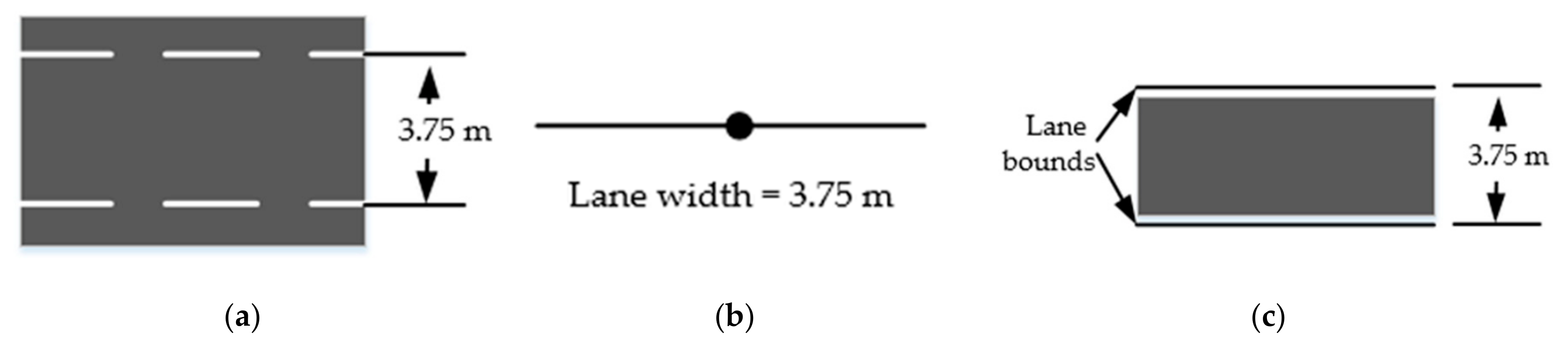
Examples of the lane logic representation: (a) a real-world lane; (b) a lane based on a node-arc model; and, (c) a lane based on a segment model.
Figure 6.
Examples of the lane logic representation: (a) a real-world lane; (b) a lane based on a node-arc model; and, (c) a lane based on a segment model.

Figure 7.
Examples of a lane representation: (a) a real-world lane; (b) a lane representation by OpenDrive; and, (c) a lane representation by lanelets.
Figure 7.
Examples of a lane representation: (a) a real-world lane; (b) a lane representation by OpenDrive; and, (c) a lane representation by lanelets.


Table 1.
Sensors comparison.
| Type | Sensor(s) | Advantages | Disadvantages |
|---|---|---|---|
| Position Sensors | Single GPS |
|
|
| INS 1 |
|
| |
| Perception Sensors | Laser scanner |
|
|
| Single camera |
|
| |
| Stereo camera |
|
| |
| Multi-camera |
|
|
1 Inertial Navigation System.
Table 2.
Lane-level road geometry extraction methods.
| Type | Technique(s) | Methodology and/or Advantages | Disadvantages |
|---|---|---|---|
| Trajectories-based | Single GPS trajectories [28,46] |
|
|
| Crowdsourced GPS trajectories [56,57] |
|
| |
| 3D Point cloud-based | 3D point cloud,single threshold [32,59] |
|
|
| 3D point cloud, multi-threshold [62,63,64] |
|
| |
| 3D point cloud, CNN [65,66] |
|
| |
| GRF Images, Hough Transform [59] |
|
| |
| GRF Images, multiscale threshold segmentation [68,69] |
|
| |
| GRF Images, MSTV [76] |
|
| |
| Vision-based | Feature [75,76] |
|
|
| Model [78,79,80] |
|
| |
| CNN [84,85,86] |
|
|
© 2019 by the authors. Licensee MDPI, Basel, Switzerland. This article is an open access article distributed under the terms and conditions of the Creative Commons Attribution (CC BY) license (http://creativecommons.org/licenses/by/4.0/).
Share and Cite
MDPI and ACS Style
Zheng, L.; Li, B.; Yang, B.; Song, H.; Lu, Z. Lane-Level Road Network Generation Techniques for Lane-Level Maps of Autonomous Vehicles: A Survey. Sustainability 2019, 11, 4511. https://doi.org/10.3390/su11164511
AMA Style
Zheng L, Li B, Yang B, Song H, Lu Z. Lane-Level Road Network Generation Techniques for Lane-Level Maps of Autonomous Vehicles: A Survey. Sustainability. 2019; 11(16):4511. https://doi.org/10.3390/su11164511
Chicago/Turabian StyleZheng, Ling, Bijun Li, Bo Yang, Huashan Song, and Zhi Lu. 2019. "Lane-Level Road Network Generation Techniques for Lane-Level Maps of Autonomous Vehicles: A Survey" Sustainability 11, no. 16: 4511. https://doi.org/10.3390/su11164511
Note that from the first issue of 2016, this journal uses article numbers instead of page numbers. See further details here.