The Impact of Traffic Crashes on Urban Network Traffic Flow

Abstract

This paper aims to investigate the impact of occasional traffic crashes on the urban traffic network flow. Toward this purpose, an extended model of coupled Nagel–Schreckenberg (NaSch) and Biham–Middleton–Levine (BML) models is presented. This extended model not only improves the initial conditions of the coupled models, but also gives the definition of traffic crashes and their spatial/time distribution. Further, we simulated the impact of the number of traffic crashes, their time distribution, and their spatial distribution on urban network traffic flow. This research contributes to the comprehensive understanding of the operational state of urban network traffic flow after traffic crashes, towards mastering the causes and propagation rules of traffic congestion. This work also a theoretical guidance value for the optimization of urban traffic network flow and the prevention and release of traffic crashes.

1. Introduction

A fluent urban traffic network is important for a city’s normal operation. However, with the acceleration of urbanization and the rapid development of urban road traffic, traffic crashes have increased significantly. Traffic crashes can easily cause casualties, property damage, and environmental damage. For traffic itself, traffic crashes can lead to traffic congestion, reduced road capacity, and increased travel time, fuel consumption, and environmental pollution. Urban traffic management is concerned with ways to reduce the impact of traffic crashes on urban road networks and ensure the efficient operation of traffic.

In order to solve this problem, scholars have proposed a large number of models from a variety of perspectives, and have made some achievements. Based on the research scope, these models can be roughly divided into macro models and micro models. The macro models mainly focus on the macro impact and predictive prevention of traffic accidents, while the micro models focus on the characteristics of accidents, their causes, influencing factors, and other aspects.

Most macro models are based on existing mathematical and statistical or network models to analyze the macro-level characteristics of crashes [1,2,3,4]. The conclusions obtained can help to obtain the main factors affecting crashes at the macro level, and then propose traffic safety control measures accordingly. Generally, micro-level models can better reflect the propagation mechanism of traffic crashes and their impact on traffic flow. The micro-level simulation analysis of road traffic flow after crashes mainly includes traffic flow dynamics models [5,6], car-following models [7,8,9], and cellular automata (CA) models [10]. Among them, the cellular automata model is the most popular because it is computer-friendly and can flexibly modify its rules to cover a variety of real traffic conditions (e.g., crashes, lights, ramps, bottlenecks, etc.), while preserving the nonlinear behavior and other physical characteristics of the traffic flow [11]. The classic one-dimensional cellular automaton traffic flow model is the Nagel–Schreckenberg (NaSch) model [12], which is mainly used in the simulation of highway crashes [13,14]. Because an urban road network is a complex two-dimensional system consisting of many road intersections in different directions, one-dimensional models are not applicable. Therefore, scholars have tried to establish two-dimensional CA models to describe urban road traffic. In 1992, Biham, Middleton, and Levine proposed the first two-dimensional traffic situation CA model [15] (i.e., the BML model) to simulate the formation and propagation rules of traffic congestion in an urban two-dimensional network, and found that it could identify the key factors of urban traffic flow phase transitions (e.g., traffic density). Later, scholars made many improvements to the BML model in order to study urban road traffic crashes by considering many factors, such as average vehicle speed, traffic signals, and so on [16,17]. The BML model can simulate the operation of an actual intersection signal, but it does not consider the road-connecting intersections, and its rules are too simple to simulate some more subtle features. From these viewpoints, in 1999, Chowdhury and Schadschneider proposed the ChSch model, which coupled the classical one-dimensional NaSch model and the two-dimensional BML model for the study of urban road traffic, and achieved good results [18].

Golob et al. studied the relationship between highway accidents and weather, lighting, and other factors, and concluded that the type of collision is strongly related to median traffic speed and to temporal variations in speed in the left and interior lanes [19]. They then developed a method to determine how crash characteristics are related to traffic flow conditions at the time of occurrence [20]. Aljanahi et al. pointed out that there is an apparent decrease in the rate of crashes if the percentage of heavy vehicles increases, with the speed distribution held constant [21]. Hiselius’s research draws a similar conclusion: as the number of trucks increases on the road, the number of crashes decreases [22]. Therefore, compared with trucks, cars are more likely to cause traffic crashes. Additionally, strengthening the management of cars can effectively improve road safety. Zhu et al. presented a highway traffic model with a blockage induced by an accident car, and concluded that the accident car not only caused a local jam behind it, but also caused vehicles to cluster in the bypass lane [23]. By considering the influence of traffic crashes and the maintenance of highway sections on traffic flow, Qian et al. analyzed highway traffic flow under the lane control when an accident occurs, and found that within a certain density range, the longer the blocked time and the length of the blocked section, the greater the influence of traffic flow [24]. For the prevention of road traffic crashes, research results show that improving roadway width, pedestrian facilities, and access management are effective in reducing road traffic crashes [25]. It has also been verified that charging vehicles for access to the central city during peak hours can sharply reduce both the number of crashes and the crash rate [26]. Scholars have also analyzed the influence of bad weather [27], road conditions, and building environment on crashes [28,29,30], as well as the externality of traffic crashes and its relationship with hourly traffic flow [31,32,33,34].

The above-mentioned articles have carried out in-depth analyses of the characteristics, predictions, influences, and evaluations of traffic crashes from different aspects, and obtained some good results. However, these studies are mainly aimed at highway traffic flow, while urban road networks are mainly weaves of a large number of roads in different directions, there are many intersections and signal lights, and the traffic organization is more complicated. The above research results are no longer applicable in this situation. Therefore, some scholars have tried to extend the research on highway traffic crashes to urban networks. For instance, Nagatani believes that the location of traffic crashes will induce traffic congestion, which will delay the forward movement of the rear vehicles. The delay time of traffic crashes is the main factor determining the range of impact time. Based on this idea, the operational status of urban traffic networks for single traffic crashes has been studied [35,36,37]. Yao et al. presented the susceptible-infected-susceptible (SIS) model and obtained the analytical expression of the critical value of delay spread, which provided basic theoretical guidance to prevent the large-area delays of urban road traffic network caused by disruptive traffic crashes [38]. However, the above studies mainly analyzed the impact of crashes on urban road networks from a macroscopic perspective, but fail to make a more detailed analysis combined with the traffic flow phase. In urban road traffic networks, several pressing questions remain. What are the impacts of traffic crashes sites, time of occurrence, road traffic density, and other factors on traffic flow? How can targeted measures be taken to reduce these adverse effects and improve traffic efficiency, so as to provide a theoretical basis for traffic management departments to formulate policies? In this paper, considering that the two-dimensional cellular automaton ChSch model has a natural advantage for studying urban road traffic flow, we introduce traffic crashes into the model and obtain an new extended model coupling the NaSch and BML models to simulate the impact of traffic crashes on urban traffic flow itself, by analyzing the traffic flow characteristics under different time and space conditions of crashes, the change rules of different traffic flow phases and traffic parameters are obtained, and suggestions are put forward regarding traffic operation and the management of urban road networks under crash conditions.

2. Model

The extended model is defined on a two-dimensional square lattice of sites with periodic boundary conditions, which is the simplification of an urban traffic network. Each site has three states, namely, either occupied by a car moving downwards, a car moving to the right, or empty. A horizontal arrow pointing to the right represents vehicles moving to the right, and a vertical downward arrow represents vehicles moving downward. The model updates synchronously, and does not allow vehicles to overtake. All traffic lights (which are only green or red in this model) have the same cycle and run synchronously. The roads are divided into sections, and traffic lights are divided into nodes in this model.

First, we define a traffic crash. Using Nagatani’s idea of traffic crashes [35], the vehicle is delayed by a certain amount of time before it can pass the accident location, $t_1$ is used to describe the time required to deal with traffic crashes and the impact caused by traffic crashes on other vehicles in the traffic network. Other variables are given as below:

• $\rho$—Density of the initial traffic network;
• $T$—Simulation time;
• $T_1$—Cycle of traffic lights;
• $T_g$—Green light time;
• $T_r$—Red light time;
• $T_g=T_r=0.5\times T_l$;
• $P_1$—The probability of randomization;
• $V_{\max }$—The maximum speed;
• $n$—Number of crashes;
• $L$—Side length of the lattice;
• $r_l$—The length of each road section;
• $r_n$—Number of sections;
• $R_l$—Length of the road;
• $R_l=r_l\times r_n$.

So, the size of the lattice is $L\times L=R_l\times R_l$.

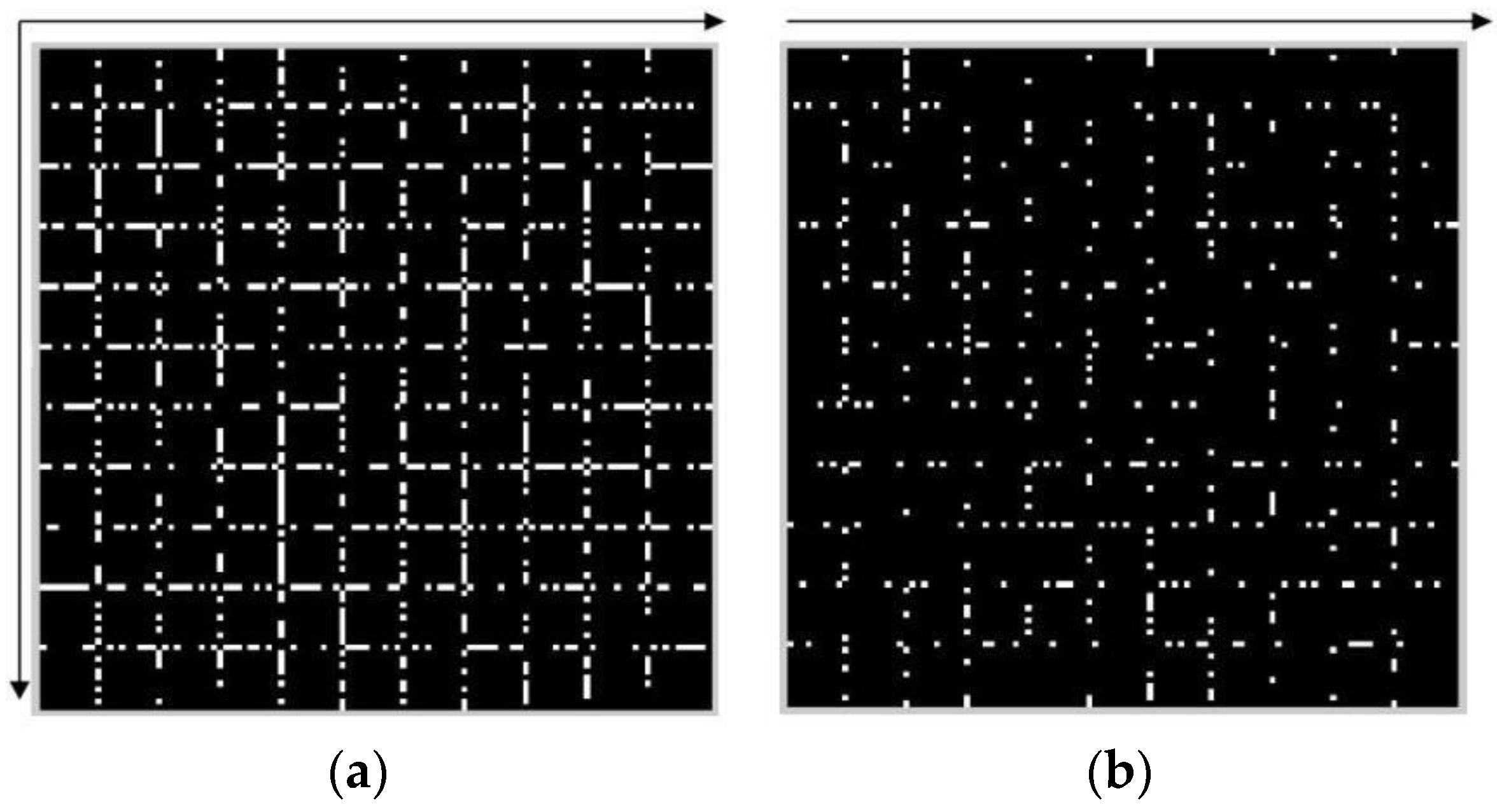
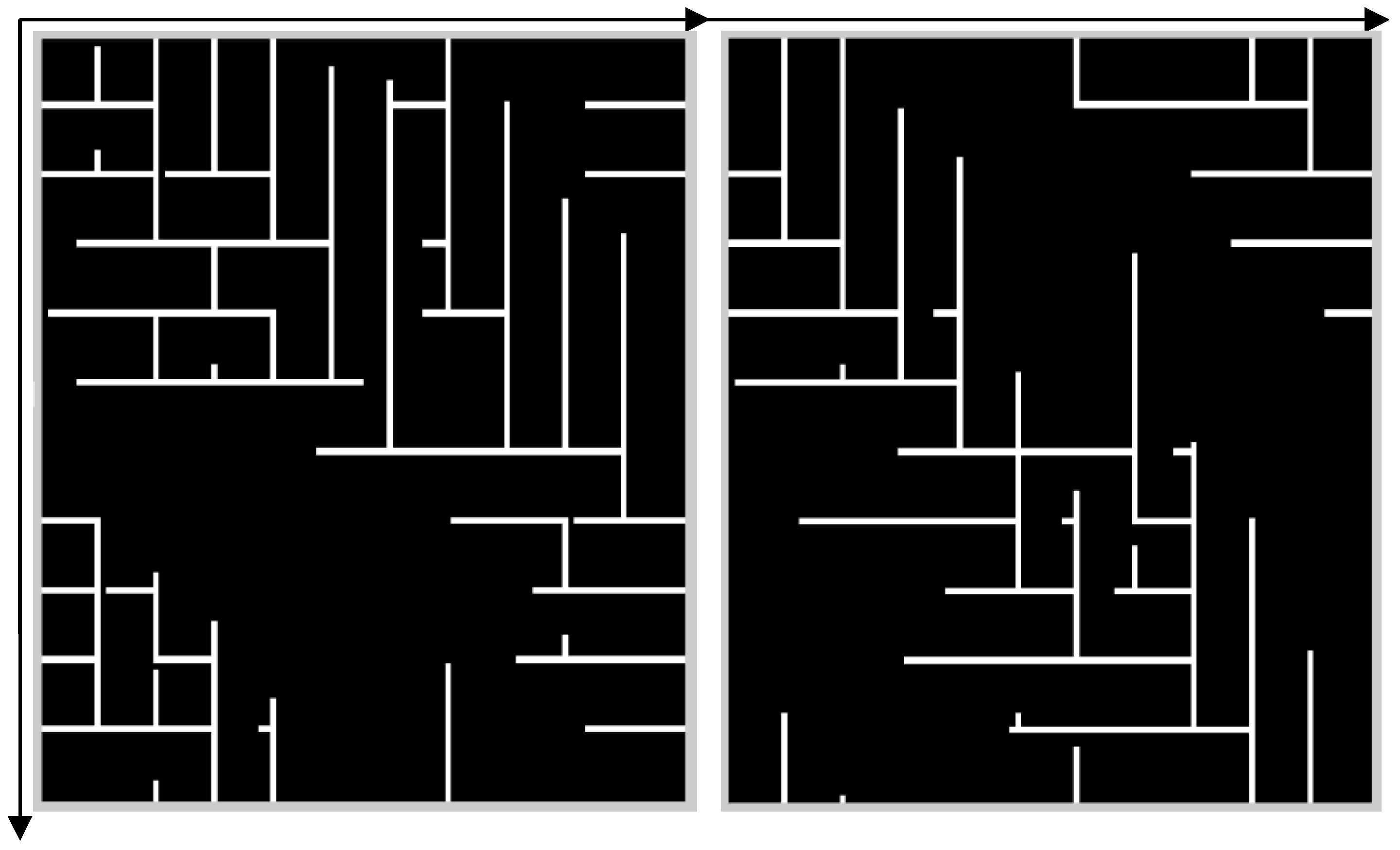
Figure 1 shows the operational states of road network traffic flow at different initial densities ($\rho =0.5$, $\rho =0.3$, respectively) when traffic crashes occur at the center of the road network. Figure 1a shows the case when $L=110$, $n=1$, and $\rho =0.5$, and Figure 1b shows the case when $L=110$, $n=1$, and $\rho =0.3$. The white points represent vehicles, in the vertical direction driving downward, and in the horizontal direction driving to right. It is clear that the road network on the left shows congestion at most intersections, with only a few vehicles moving freely, and the basic traffic function failure caused by congestion has led to traffic congestion and delay has been increased. On the right figure, it can be found that the entire traffic network flow is in the free-flow state, and most vehicles can travel at maximum speed. Thus, the operational status of the road network is related to the initial density. With the increase of the traffic networks’ density, vehicle congestion and delays worsen. Therefore, there is a critical density in the road network. When the initial density is less than this critical density, vehicles can travel freely, and when the initial density is greater than this critical density, the road network easily forms a global traffic congestion by itself.

3. Results and Analysis

To eliminate the random impacts of different initial conditions on the simulation results, we re-averaged 100 samples. When the sample ran $2\times {10}^3$ time steps, the simulation system made an average of all $2\times {10}^3$ time steps. If there is no special explanation, the relevant parameters in the simulation were taken as follows: $L=110$, $T_l=30$, $T_g=T_r=0.5\times T_l=15$, $R_l=110$, $r_l=10$, $r_n=11$, $P_1=0.3$, $V_{\max }=3$.

In the odd time steps of $T_g$ or $T_r$, the horizontal east–west direction traffic lights are green and the vertical north–south direction traffic lights are red. In the even time steps of $T_g$ or $T_r$, the opposite is true. The model uses periodic boundary conditions, which ensures that the traffic density $\rho$ of the road network is fixed.

When the number of road crashes $n$ > 1, $\alpha$ and $r$ are respectively used to indicate the angle (according to the counterclockwise rotation) and the straight line distance of the accident point from the center accident point, in order to determine the location of the crash from the road network center. In numerical simulation, the vehicle average speed of the entire network was obtained by the following equation:

$$\overline{V}=\frac{{\displaystyle \sum _{t=1}^T{\overline{V}}_e}+{\displaystyle \sum _{t=1}^T{\overline{V}}_s}}{T},$$

(1)

where $\overline{V}$ is the average speed over all time steps, ${\overline{V}}_e$ is the average speed of all vehicles moving to the right, ${\overline{V}}_s$ is the average speed of all vehicles moving downward, $T$ is the total time steps in the simulation, and $t$ denotes a single time step.

3.1. Global Clustering

On the basis of above model, the simulation was conducted under the above initial conditions. At the beginning, vehicles which were only allowed to move to the right or downward were respectively randomly distributed on the horizontal and vertical roads. Parallel computing and location updating were performed according to the rules given above. After the initial unstable state gradually moved towards a steady state, we found that the traffic flow changed from the free flow phase to a completely congested phase.

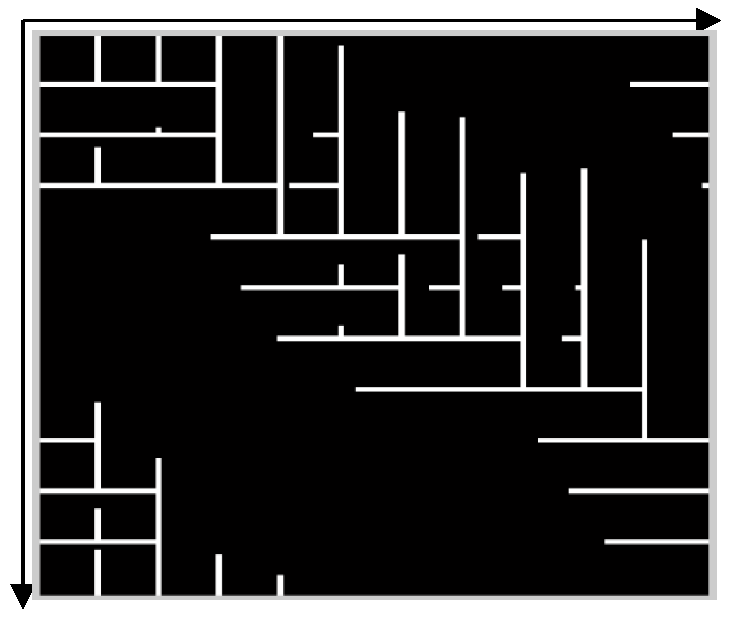
After many simulations, we found that in the extended coupled model, the operational state of the road network was closely related to the initial density. When the initial state density was less than a certain critical value, the road network was in the free flow state. When the initial density was greater than this value, it very easily spontaneously formed a completely congested configuration. A certain configuration of urban traffic network congestion is called clustering. Global clustering often means the congestion of the whole urban road traffic network. At this time, all the vehicles in the road network are closely connected, and there is no gap between the front and rear vehicles. That is to say, the formation of a global cluster is very similar to the global clustering in the BML model. The complete congestion configuration in the extended ChSch model is shown in Figure 2. In the Figure, the white lines are the vehicle queues. It can be seen that the road network system had formed clusters from the upper-left corner to the lower-right corner. This configuration makes it so that all the vehicles in the road network are unable to move forward, causing the entire traffic network to collapse. We found that in the BML model, the vehicle clusters from the lower-left corner to the upper-right corner were formed by the vehicles traveling northward and the vehicles traveling eastward. Therefore, it can be seen that the direction of the traffic flow determines the final global cluster configuration.

3.2. The Relationship between Global Congestion and Road Network Density

From the above numerical simulation, it could be found that when the initial density $\rho =0.4$, the road network was completely blocked by itself. However, with changes of $\rho$, the global clustering may not occur. That is because when the initial density was small, all vehicles could move freely and the entire traffic network was in a free-flow state. This shows that the global congestion and road network density are related.

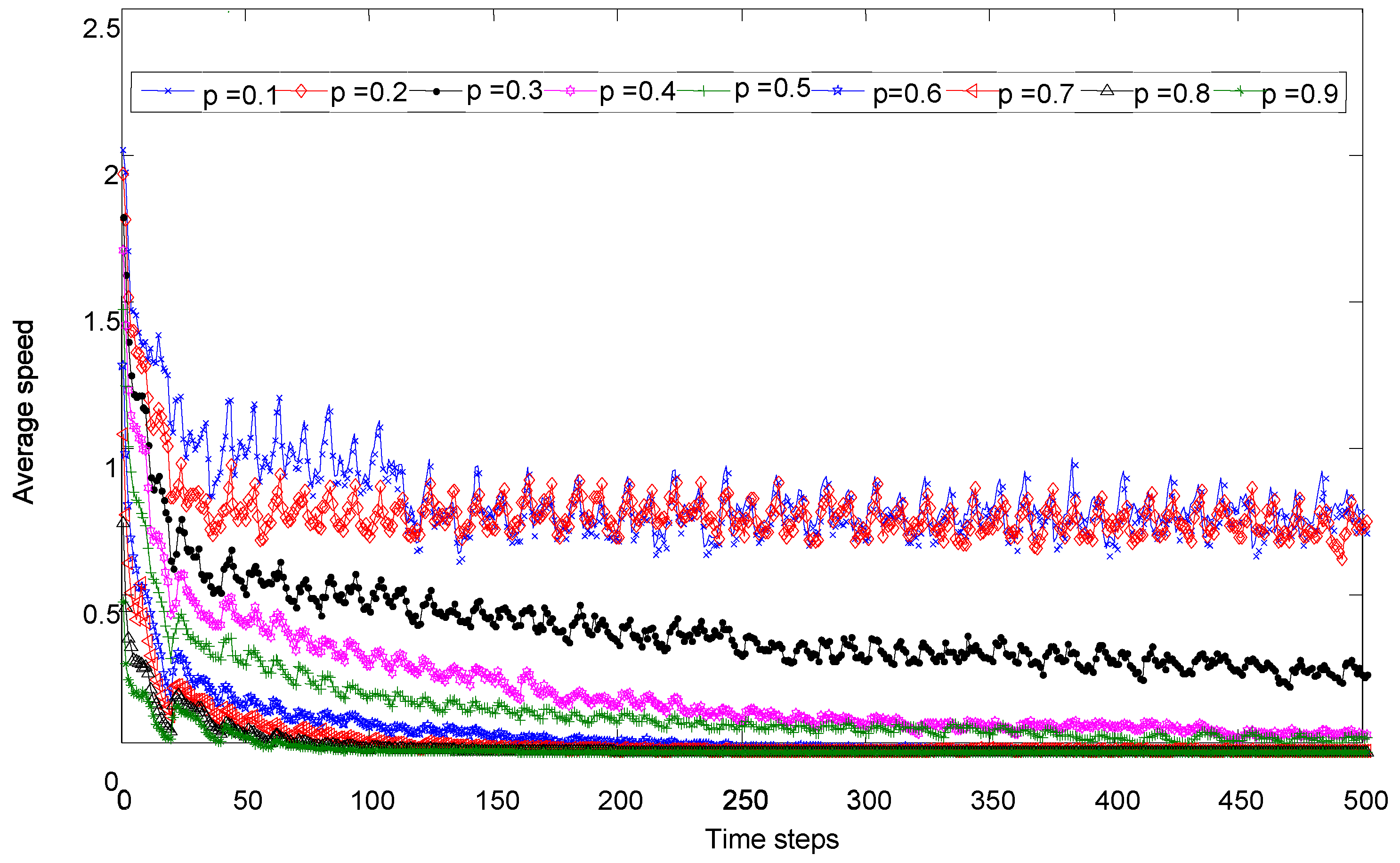
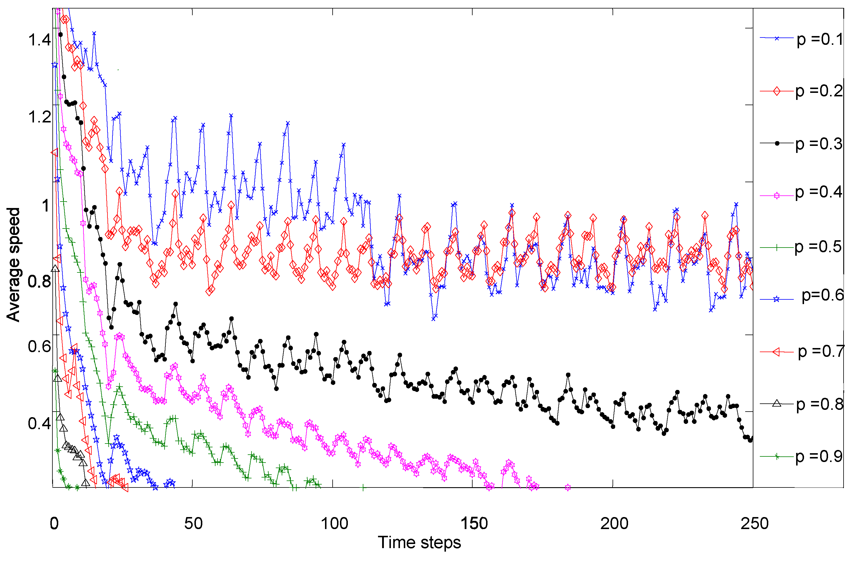
By changing the initial traffic density, the average speed changed accordingly (as shown in Figure 3 and Figure 4), and finally we found that the critical density value caused global congestion. The initial density of the road network was set to 0.1, 0.2, 0.3, 0.4, 0.5, 0.6, 0.7, 0.8, or 0.9, respectively, and meanwhile we studied corresponding changes to the average speed. When the initial traffic density was less than 0.2, the average speed obtained was significantly greater than the average speed under other initial density conditions, and global clustering did not occur. When the initial density was equal to 0.3, in 500 time steps, some vehicles were blocked, but some vehicles could travel freely. When the initial density was greater than 0.3, the road network was easily blocked. This indicates that there was a critical initial density that changes traffic flow from free-flow to global congestion near $\rho \in [0.2,0.3]$. In Figure 4, when the initial density was greater than or equal to 0.5, the average speed became 0 in a very short time, which means that the entire road network was paralyzed. In order to study the influence of the spatial distribution and time distribution of accident points on the whole network more clearly, the initial density of the traffic network was set to $\rho =0.4$ for simulation calculation. Global clustering occurs under this condition.

3.3. The Impact of Crashes on the Traffic Network

In order to study the difference between the impact of crashes on the urban road traffic network and congestion caused by the network on its own, we selected a point on the road network losing its traffic function to represent the traffic crashes on the actual urban road traffic network. The simulation results are shown in Figure 5. The left figure shows the complete congestion configuration caused by crashes at the node near the center point, and the right figure shows complete congestion configuration caused by the vehicles themselves without an accident point. In the left figure, the vehicles upstream of the crash point formed an isolated congested area, indicating the accident had a greater impact on the upstream traffic, which is the same as actual traffic. In actual traffic, when an accident happens somewhere, the upstream vehicles are affected and queued up, while the downstream vehicles are basically unaffected. Instead, the upstream vehicles are prevented from entering the downstream sections due to accident, so the downstream vehicles can travel freely and the average speed of all vehicles may increase. In the right figure, the congestion area is concentrated in the middle diagonal, determined by the traveling direction of the vehicles.

We need to calculate the average speed of the urban road traffic network with or without crashes in order to study the impact of crashes on the average speed of the entire road network.

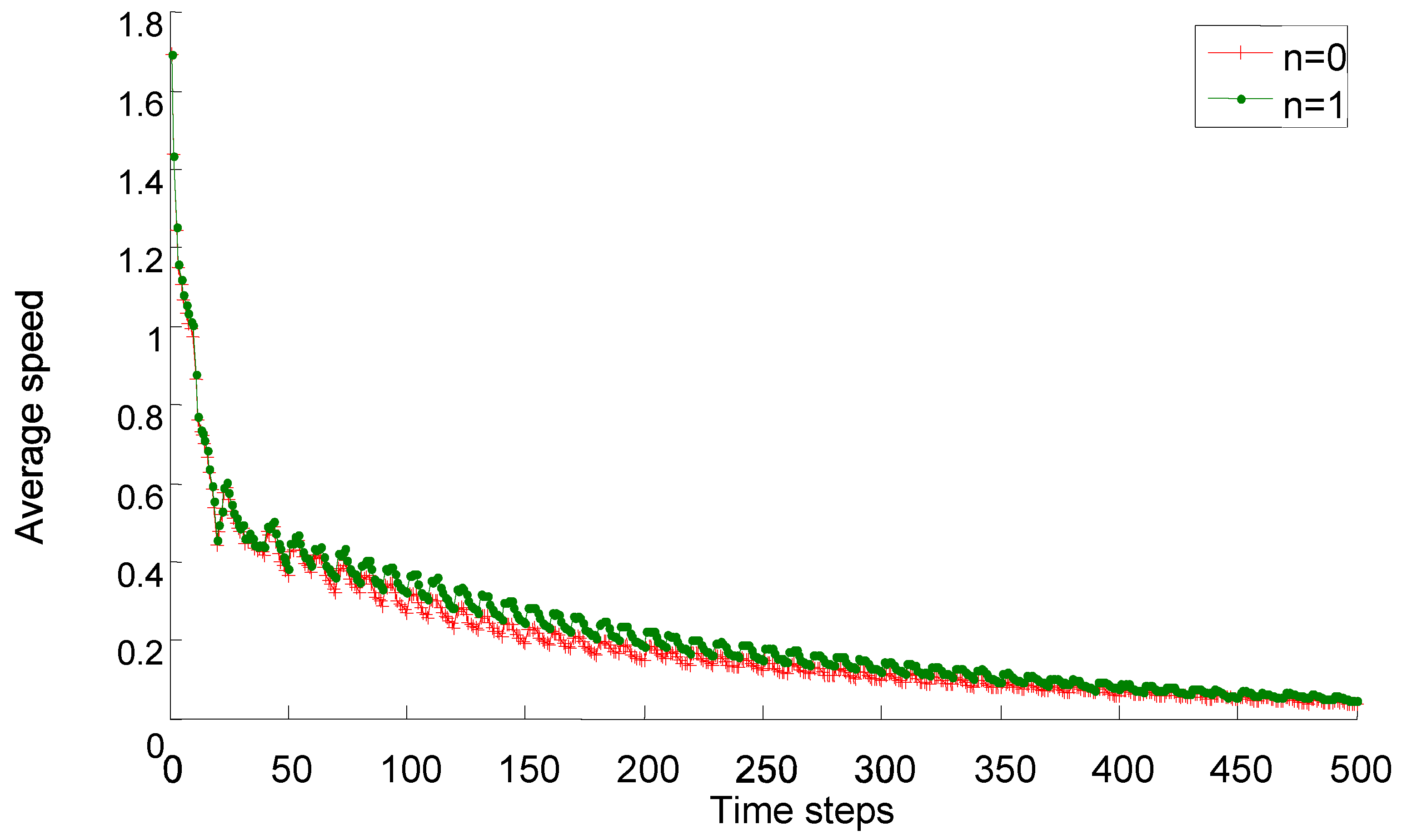
Figure 6 shows the average speed of the urban road traffic network with or without crashes. Interestingly, the average speed of the traffic network with crashes was higher than that without crashes at most time points. To further study the duration of this result, we continued to calculate the average speed of these two cases and found that the average speed of traffic network with crashes was higher than that without crashes at more than 96% of simulation time points.

This conclusion seems strange, but it is not difficult to understand. The congestion area is an isolated area. The formation of the area relatively increases the road area of vehicles in other regions, and the vehicle density on the entire road is reduced. The speed of vehicles in the non-congested areas of the road network is improved, such that the entire average speed is improved.

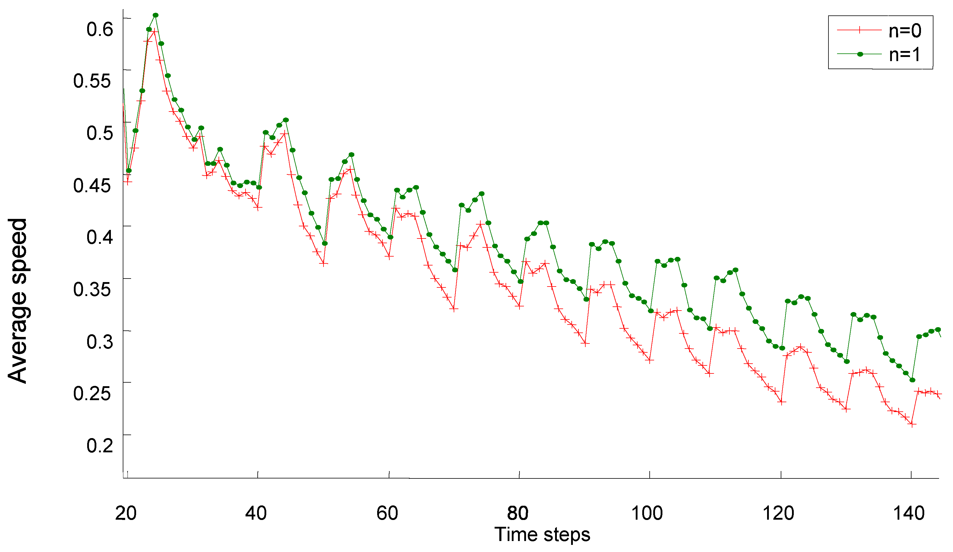
In Figure 7, the average speed became higher than that without crashes 20 time steps after the accident occurred. With the simulation, the speed difference increased continuously. This agrees with our conclusion above.

3.4. The Impact of Traffic Crashes’ Spatial Distribution on the Traffic Network

From the above conclusion of the ChSch model’s global clustering, when traffic crashes occur at different locations, the impacts on the network are also different, including the average speed of the network and congestion configurations. Next, we simulated the impact of traffic crashes’ spatial distribution on the urban road traffic network.

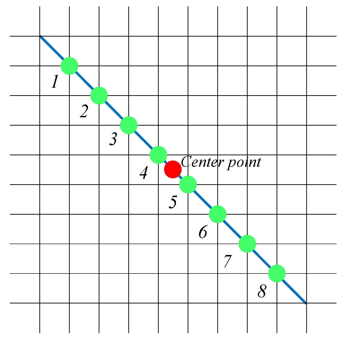
For the convenience of the research, we defined the spatial distribution of the crash points as follows. Crash points are evenly distributed on the diagonal from the upper-left corner to the lower-right corner of the road network. The location distribution of the center point and crash points on the road network is shown in Figure 8. There are four crash points on left side of the urban road traffic network’s center point, and there are four on right side as well, which we numbered from 1 to 8. In the following, we study the relationship among the location of each crash point, the average speed of the network, as well as the global congestion time in order to determine the impact of the crashes’ spatial distribution on the traffic network.

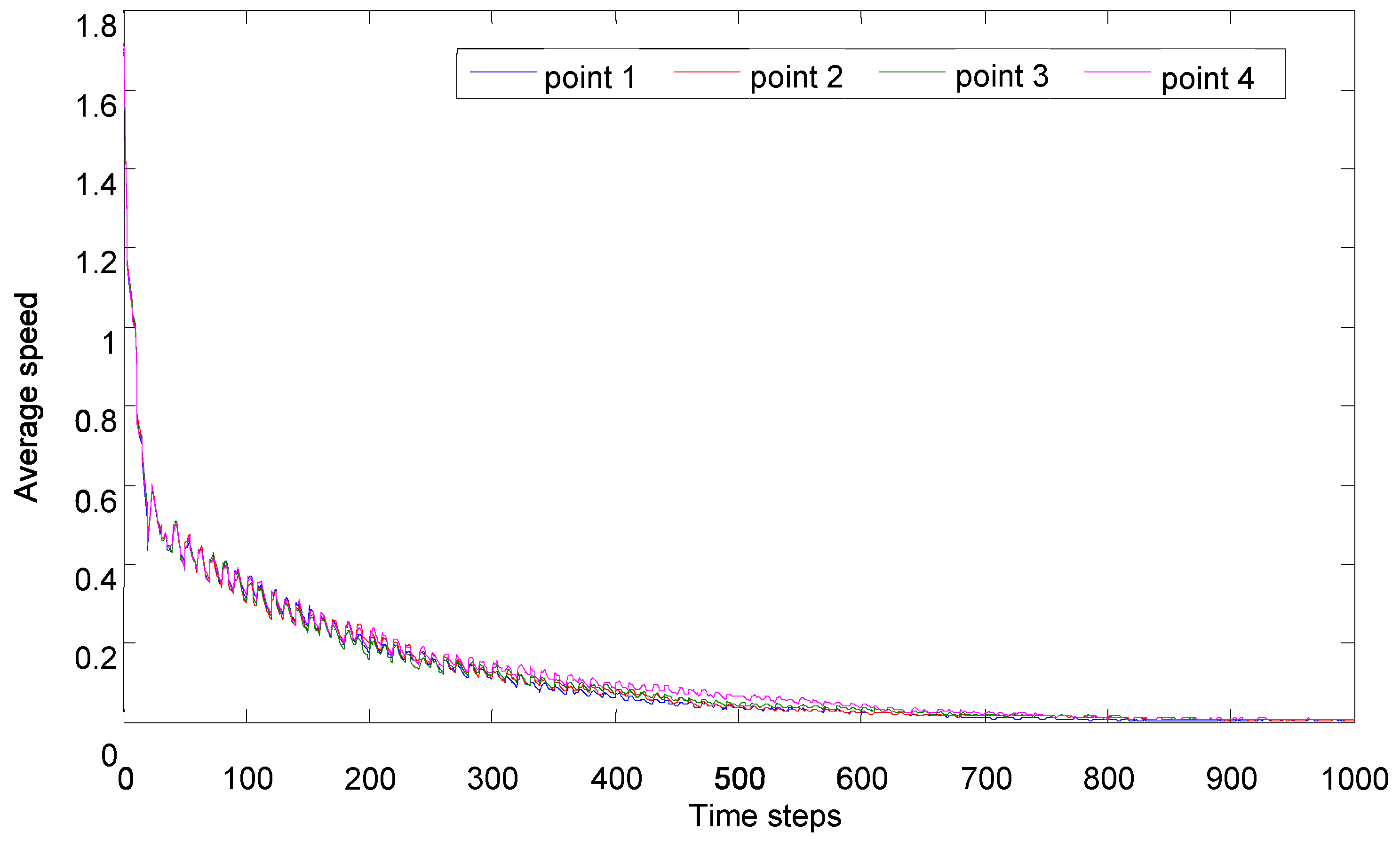
We simulated the operational status of the urban road traffic network when traffic crashes occurred at different points (from point 1 to point 8). The average speed curves of the network are shown in Figure 9, Figure 10, Figure 11 and Figure 12, which were obtained by counting the speed of the network in the above eight cases.

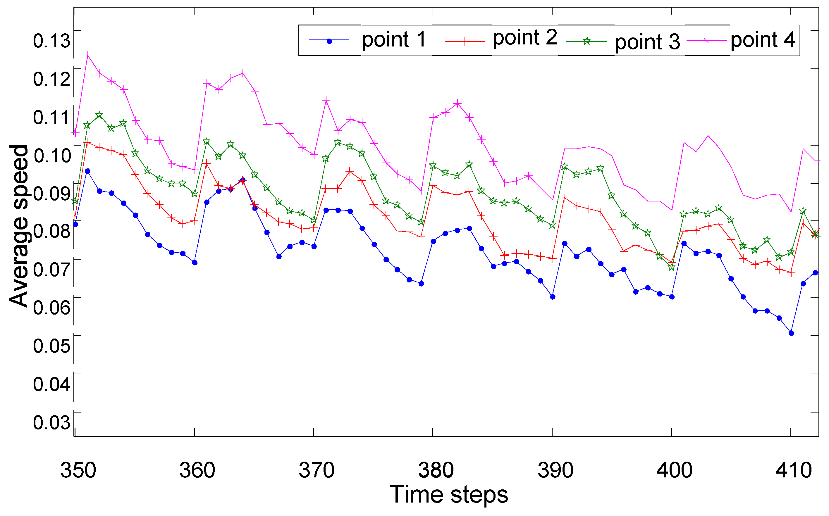
Figure 9 and Figure 10 show the simulation results of crash points one to four. At the beginning of the simulation time step, the average speed of system did not have obvious rules. As time progressed, the following phenomenon occurred. When the crash occurred at the point farthest from the city center (point 1), the average speed of the system was the lowest. When the crash occurred at point 4, which is closest to the city center, the average speed of the system reached the highest. This trend of the average speed of the system can be seen more clearly in Figure 10. This shows that the impact on the traffic network increased as distance from the center point increased, and the average speed of the urban road traffic network decreased with the distance from the center.

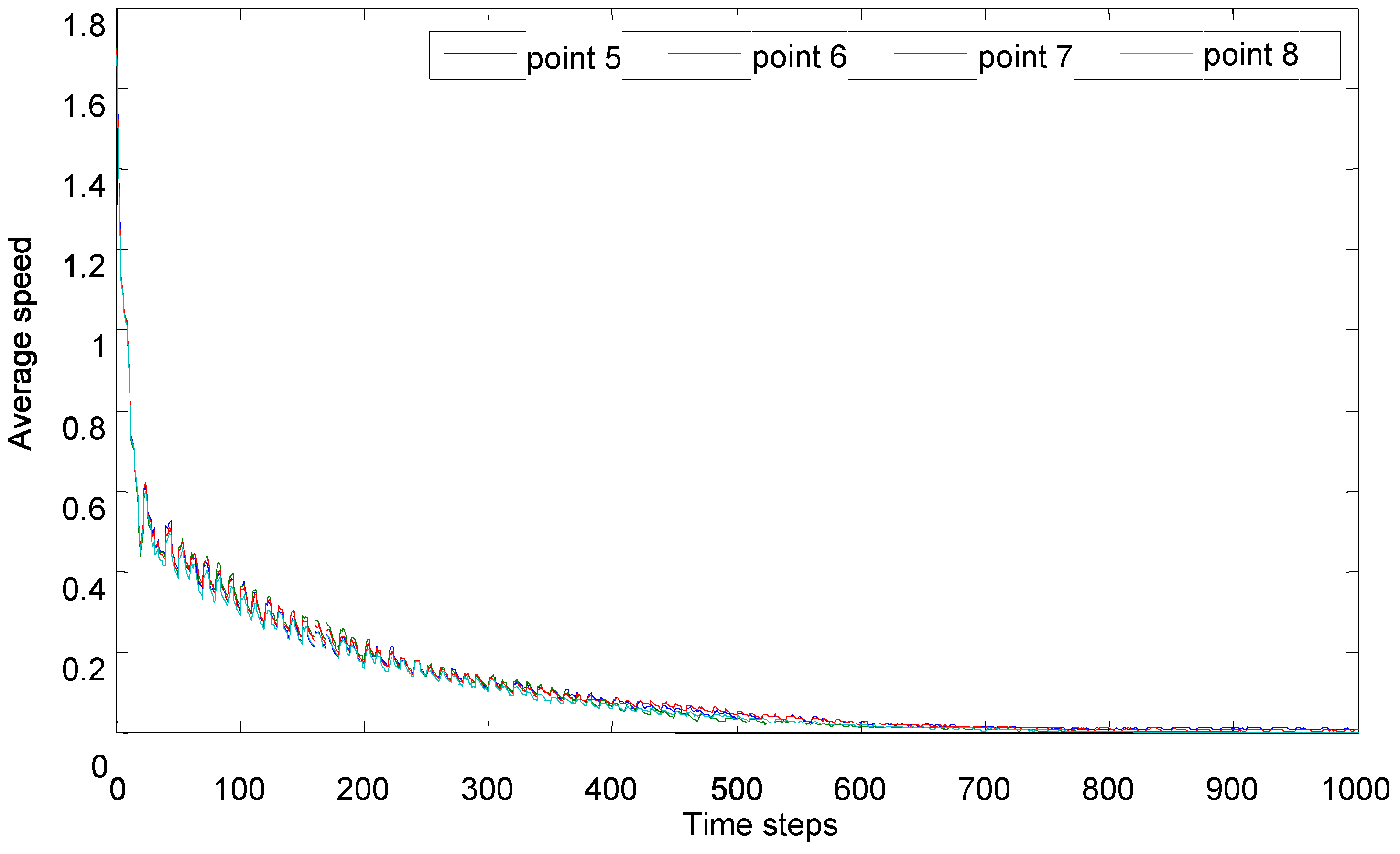
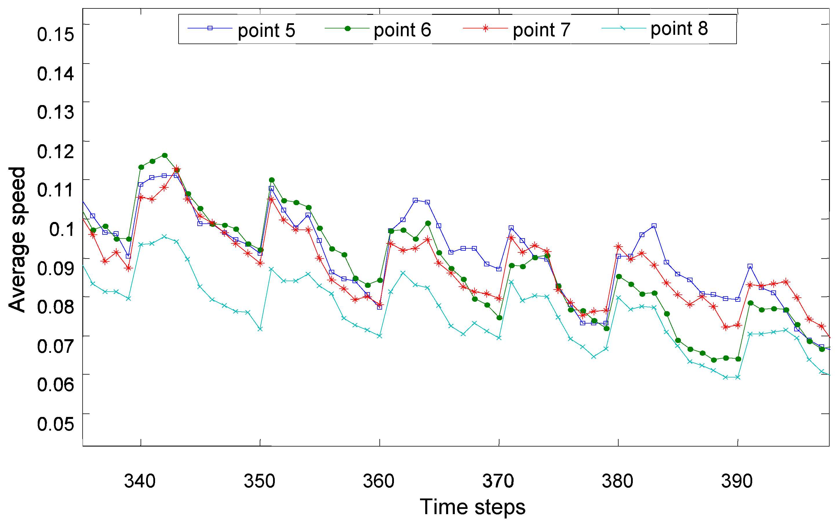
Figure 11 and Figure 12 show the average speed of the system when the crashes occurred at points 5, 6, 7, and 8, respectively. The results show that when the crash occurred at the point farthest away from the city center, the impact on the system’s average traffic flow was the greatest, and the declines of the system’s average speed were the greatest. This is because the movement direction of vehicles in the model was to the right and downward. The system formed a global congestion from the upper-left corner to the lower-right corner by itself, and the congestion points we set were just on this diagonal. Traffic crashes at points from 1 to 4 can cause congestion quickly, leaving a large amount of road space for the remaining vehicles to move freely, so the network average speed increased. The impact of crashes from points 5 to 8 was the opposite to the case of crashes from points 1 to 4.

3.5. The Impact of Traffic Crashes’ Time Distribution on the Traffic Network

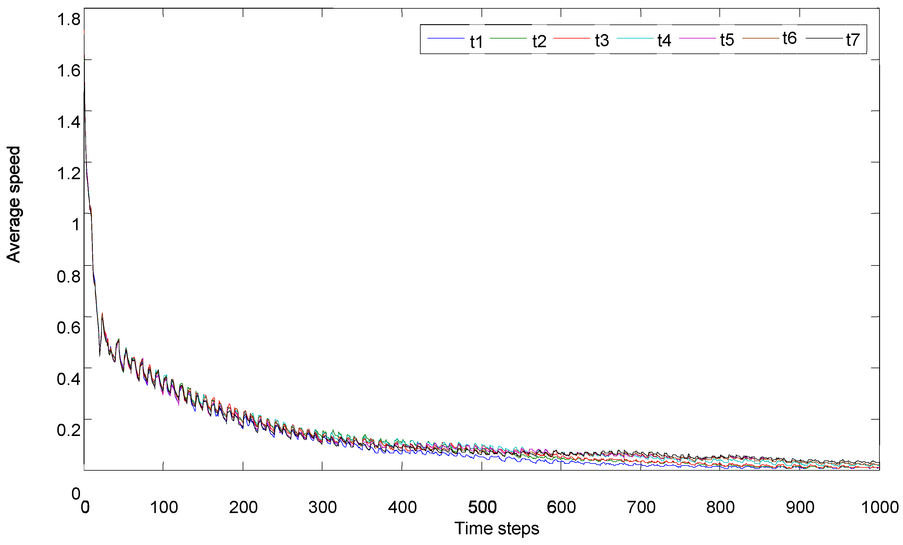
The following describes the impact of traffic crashes’ time distribution on the urban traffic network. We chose traffic crashes on point 4 in Figure 8; the time of the traffic crashes was defined as $t_{accident}$, and its values were $(t_1=1,t_2=51,t_3=101,t_4=151,t_5=201,t_6=251,t_7=301)$. That is, we evaluated the change of the system’s average speed when the traffic crashes occurred at point 4 during time step $t_{accident}$. The following simulation evaluated the impact of traffic crashes’ time distribution on the traffic network’s average speed.

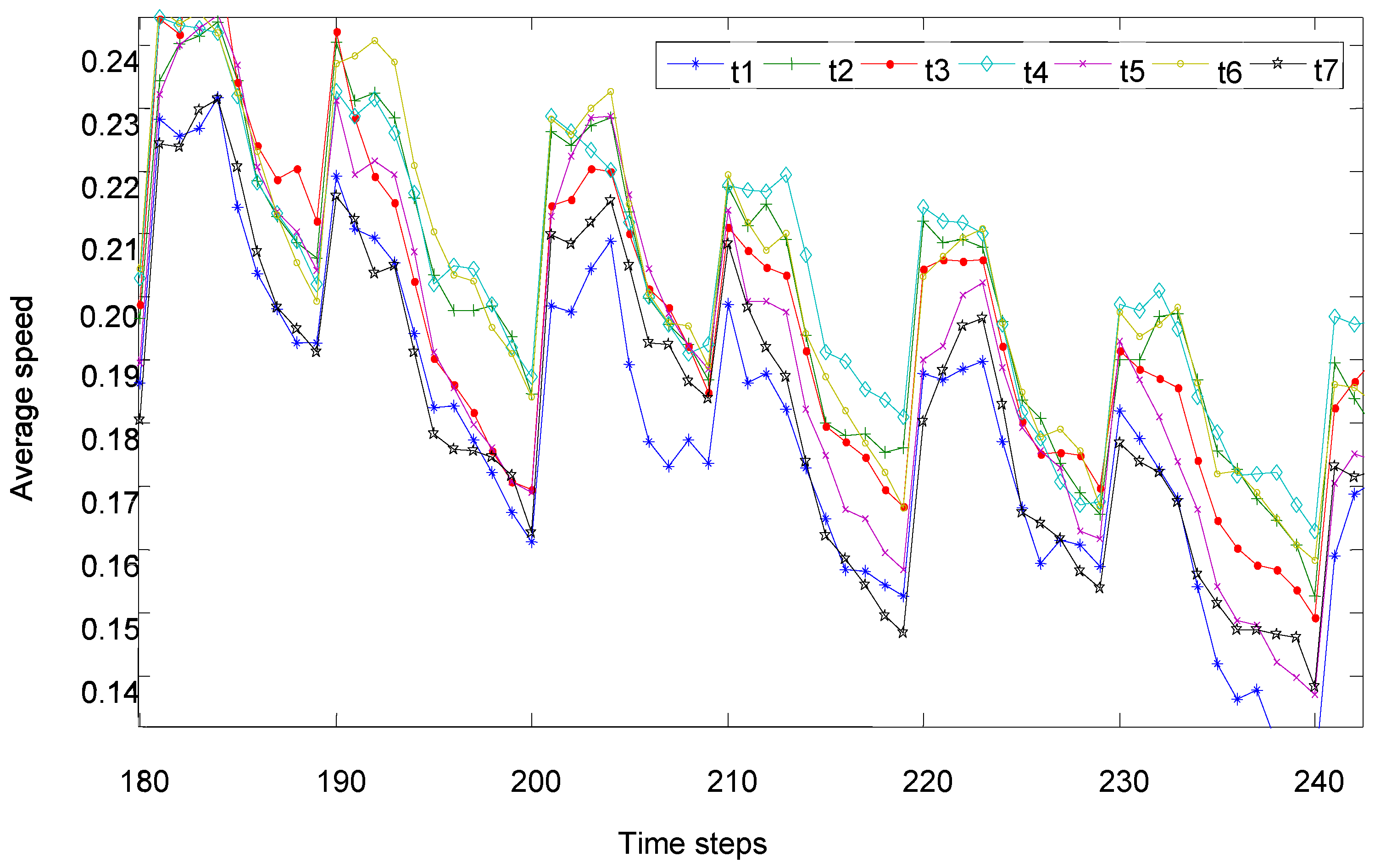
From Figure 13 and Figure 14, the impact on entire traffic flow first increased and then decreased as the time of traffic crash was pushed forward. This shows that the time of traffic crashes occurring at same place had some regular impact on the road network. Before a wide range of traffic congestion appeared, congestion which happened in advance could cause local congestion, which makes it more difficult for vehicles in other areas to form congestion. However, with the gradual increase of congestion in the road network, the impact of newly formed congestion points on the road network is decreased.

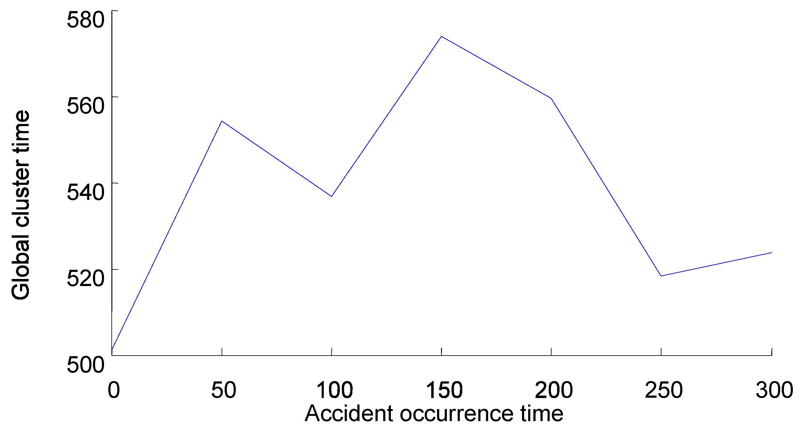
In the above two figures, it can be seen that the different times of the traffic crashes had a certain impact on the system’s average speed. So, we calculated the impact of traffic crashes occurring at different times on the global clustering, as shown in Figure 15. From this figure, when a traffic crash occurred at time step $t_1=1$, the entire road network was completely blocked after the road network ran 503 time steps, and when a crash occurred at time step $t_4=151$, the longest time of the global cluster formed was 574 time steps, but at time steps $t_5=201$, $t_6=251$, and $t_7=301$, the global cluster time gradually decreased. This is because before the road network gradually formed a certain range of traffic congestion, and traffic jams which occurred in advance could cause local congestion. Vehicles in other areas could thus take up more space to travel freely, making it more difficult to form congestion. However, with the gradual formation of road network congestion, the impact of new congestion points on the road network decreased. This means with delay of the crash, the traffic flow of the entire road network first increased and then decreased. Therefore, traffic crashes occurring at different times in the same place had different impacts on the road network’s operational status. The later the crash happened, the smaller its impact on the road network.

4. Conclusions

Occasional traffic crashes are one of the major causes of congestion in urban traffic networks. In this paper, we introduced traffic crashes into an extended coupled model of NaSch and BML models, and studied the impact of the time and spatial distribution of traffic crashes on the urban road network. The simulation results were as follows.

When the initial traffic density of the urban road network was not greater than 0.2, the average speed of vehicles traveling was obviously greater than that under other density conditions, and there was no global clustering. The initial traffic density of the urban road network had a critical density near the value of $\rho \in [0.2,0.3]$. When the system’s initial density was greater than the critical density, it made the traffic flow change from the free-flow state to the completely congested state. Hence, urban traffic managers and policy makers should control the number of vehicles in the road network to avoid the transition of traffic flow phase from free-flow phases to traffic jams due to the high traffic density.

The location of the traffic crashes relative to the road network center had a differential impact on the traffic network. The impact on the traffic network was the greatest when the crash occurred at the point farthest away from the center point, and the average speed of the traffic network was the lowest in this case. This is because the road network is denser as distance to the center of the city decreases, and there is a stronger ability to withstand crashes; thus, the congestion caused by crashes can be quickly evacuated from other adjacent road sections. Roads farther away from the center of the city are the opposite. Therefore, compared with the city center, this situation requires that traffic management departments strengthen the daily management of the surrounding road sections of the city and improve the efficiency of crash handling so as to avoid the great impact of traffic congestion caused by crashes in the surrounding sections of the city on the urban traffic as a whole.

Traffic crashes occurring at different times at the same place had a certain impact on road network operational states. The later the accident happened, the smaller the impact on the road network. For congestion caused by traffic crashes, if it was not resolved in time, the longer the congestion lasted, and the greater the impact on the entire road traffic. The earlier the crash occurred, the greater the possibility of this situation arising. Therefore, traffic management departments need to improve the ability to detect and dispose of traffic crashes, and reduce the duration of congestion caused by crashes, so as to reduce their impact on the entire urban traffic network.

References

- Guo, L.; Zhou, J.; Dong, S.; Zhang, S.-C. Analysis of Urban Road Traffic Accidents Based on Improved K-means Algorithm. China J. Highway Trans. 2018, 31, 270–279. [Google Scholar]
- Vorko-Jović, A.; Jović, F. Macro model prediction of elderly people’s injury and death in road traffic accidents in Croatia. Accid. Anal. Prev. 1992, 24, 667–672. [Google Scholar] [CrossRef]
- Qin, L.; Shao, C. Macro prediction model of road traffic accident based on neural network and genetic algorithm. In Proceedings of the Second International Conference on Intelligent Computation Technology & Automation, Zhangjiajie, China, 10–11 October 2009; Volume 1, pp. 354–357. [Google Scholar]
- Song, C.J.; Li, Q.Y. The prediction model of macro-road traffic accident basing on radial basis function. Appl. Mech. Mater. 2011, 97–98, 981–984. [Google Scholar]
- Wei, L.; Chen, T.; Qiang, Y.U. Three-dimensional vehicle dynamics model for road traffic accident simulation and reconstruction. J. Traffic Transp. Eng. 2003, 3, 88–92. [Google Scholar]
- Dadashova, B.; Ramírez, B.A.; Mcwilliams, J.M.M.; Izquierdo, F.A. Dynamic statistical model selection: Application to traffic accident analysis in Spain. Procedia Soc. Behav. Sci. 2012, 48, 642–652. [Google Scholar] [CrossRef]
- Chen, B.; Wei, L. Car-following model under influence of expressway accident. J. Traffic Transp. Eng. 2006, 6, 103–108. [Google Scholar]
- Brill, E.A. A car-following model relating reaction times and temporal headways to accident frequency. Transp. Sci. 1972, 6, 343–353. [Google Scholar] [CrossRef]
- Cong, Z.; Liu, W.; Tan, F. Feedback control strategy of a new car-following model based on reducing traffic accident rates. Transp. Plan. Technol. 2018, 39, 1–12. [Google Scholar]
- Kong, L.P.; Li, X.G.; Lam, W.H.K. Traffic dynamics around weaving section influenced by accident: Cellular automata approach. Int. J. Mod. Phys. C 2015, 26, 1550026. [Google Scholar] [CrossRef]
- Wolfram, S. Statistical mechanics of cellular automata. Rev. Mod. Phys. 1983, 55, 601–644. [Google Scholar] [CrossRef]
- Nagel, K.; Herrmann, H.J. Deterministic models for traffic jams. Phys. A 1993, 199, 254–269. [Google Scholar] [CrossRef] [Green Version]
- Bentaleb, K.; Lakouari, N.; Marzoug, R.; Ez-Zahraouy, H.; Benyoussef, A. Simulation study of traffic car accidents in single-lane highway. Phys. A Stat. Mech. Its Appl. 2014, 413, 473–480. [Google Scholar] [CrossRef]
- Moussa, N. Car accidents in cellular automata models for one-lane traffic flow. Phys. Rev. E 2003, 68, 036127. [Google Scholar] [CrossRef]
- Biham, O.; Middleton, A.; Levine, D. Self-organization and a dynamical transition in traffic-flow models. Phys. Rev. A 1992, 6124–6127. [Google Scholar] [CrossRef]
- Liu, X.M.; L, Y.H.; Chen, Y.M.; Zheng, S.H.; Li, Z.X. Road net traffic status analysis under traffic accident based on improved BML model. J. Transp. Syst. Eng. Inf. Technol. 2010, 10, 122–129. [Google Scholar]
- Marzoug, R.; Ez-Zahraouy, H.; Benyoussef, A. Simulation study of car accidents at the intersection of two roads in the mixed traffic flow. Int. J. Mod. Phys. C 2015, 26, 1550007. [Google Scholar] [CrossRef]
- Chowdhury, D.; Schadschneider, A. Self-organization of traffic jams in cities: Effects of stochastic dynamics and signal periods. Phys. Rev. E 1999, 59, 1311. [Google Scholar] [CrossRef]
- Golob, T.F.; Recker, W.W. Relationships among urban freeway accidents, traffic flow, weather, and lighting conditions. J. Transp. Eng. 2003, 129, 342–353. [Google Scholar] [CrossRef]
- Golob, T.F.; Recker, W.W. A method for relating type of crash to traffic flow characteristics on urban freeways. Transp. Res. Part A Policy Pract. 2004, 38, 53–80. [Google Scholar] [CrossRef]
- Aljanahi, A.A.M.; Rhodes, A.H.; Metcalfe, A.V. Speed, speed limits and road traffic accidents under free flow conditions. Accid. Anal. Prev. 1998, 31, 161–168. [Google Scholar] [CrossRef]
- Hiselius, L.W. Estimating the relationship between accident frequency and homogeneous and inhomogeneous traffic flows. Accid. Anal. Prev. 2004, 36, 985–992. [Google Scholar] [CrossRef]
- Zhu, H.B.; Lei, L.; Dai, S.Q. Two-lane traffic simulations with a blockage induced by an accident car. Physics A 2009, 388, 2903–2910. [Google Scholar] [CrossRef]
- Qian, Y.S.; Zeng, J.W.; Du, J.W.; Liu, Y.F.; Wang, M.; Wei, J. Cellular automaton traffic flow model considering influence of accidents. Acta Phys. Sin. 2011, 60, 103–112. [Google Scholar]
- Berhanu, G. Models relating traffic safety with road environment and traffic flows on arterial roads in addis ababa. Accid. Anal. Prev. 2004, 36, 697–704. [Google Scholar] [CrossRef]
- Green, C.P.; Heywood, J.S.; Navarro, M. Traffic accidents and the london congestion charge. J. Public Econ. 2016, 133, 11–22. [Google Scholar] [CrossRef]
- Jaroszweski, D.; McNamara, T. The influence of rainfall on road accidents in urban areas: A weather radar approach. Travel Behav. Soc. 2014, 1, 15–21. [Google Scholar] [CrossRef] [Green Version]
- Zhang, Z. Road conditions, traffic environment and traffic crashes analysis. J. Highw. Transp. Res. Dev. 2000, 17, 56–59. [Google Scholar]
- Snyder, J.C. Environmental determinants of traffic accidents: An alternate model. Transp. Res. Rec. 1971, 486, 11–18. [Google Scholar]
- Gomes, S.V. The influence of the infrastructure characteristics in urban road accidents occurrence. Accid. Anal. Prev. 2013, 60, 289–297. [Google Scholar] [CrossRef]
- Dickerson, A.; Vickerman, P.R. Road accidents and traffic flows: An econometric investigation. Econ. New Ser. 2000, 67, 101–121. [Google Scholar] [CrossRef]
- Martin, J.L. Relationship between crash rate and hourly traffic flow on interurban motorways. Accid. Anal. Prev. 2002, 34, 619–629. [Google Scholar] [CrossRef]
- Cedar, A.; Livneh, M. Relationships between road accidents and hourly traffic flow—I: Analyses and interpretation. J. Saf. Res. 1983, 14, 19–34. [Google Scholar] [CrossRef]
- Ceder, A. Relationships between road accidents and hourly traffic flow—II: Probabilistic approach. Accid. Anal. Prev. 1982, 14, 35–44. [Google Scholar] [CrossRef]
- Nagatani, T. Effect of traffic crashes on jamming transition in traffic-flow model. J. Phys. A Gen. Phys. 1993, 26, 1015–1020. [Google Scholar] [CrossRef]
- Nagatani, T. Anisotropic effect on jamming transition in traffic-flow model. J. Phys. Soc. Jpn. 1993, 62, 2656–2662. [Google Scholar] [CrossRef]
- Nagatani, T. Jamming transition in the traffic-flow model with two-level crossings. Phys. Rev. E Stat. Phys. Plasmas Fluids Relat. Interdiscip. Top. 1993, 48, 3290–3294. [Google Scholar] [CrossRef] [Green Version]
- Yao, H.; Li, Z.; Lin, Y. Critical Boundary of Delay Spread on Urban Road Traffic Network under Disruptive Traffic crashes. J. Syst. Manag. 2017, 26, 663–669. [Google Scholar]
Figure 1.
The simulation of an urban traffic network under , : (a) ; (b) .
Figure 2.
The completely congested configuration of the urban road network under , , and number of crashes .
Figure 3.
The average speed under different .
Figure 4.
The average speed under different (0–250 time steps).
Figure 5.
The completely congested configuration of an urban road network under , , (left), and (right), respectively.
Figure 6.
The average speed under and .
Figure 7.
The average speed under and (20–140 time steps).
Figure 8.
The spatial distribution of crashes on the urban road traffic network.
Figure 9.
The average speed at different crash points.
Figure 10.
The average speed at different crash points (350–410 time steps).
Figure 11.
Figure 12.
The average speed at different crash points (340–390 time steps).
Figure 13.
Figure 14.
The average speed under different (180–240 time steps).
Figure 15.
The impact of different traffic crash occurrence times on the global cluster time.
© 2019 by the authors. Licensee MDPI, Basel, Switzerland. This article is an open access article distributed under the terms and conditions of the Creative Commons Attribution (CC BY) license (http://creativecommons.org/licenses/by/4.0/).
Share and Cite
MDPI and ACS Style
Zeng, J.; Qian, Y.; Wang, B.; Wang, T.; Wei, X. The Impact of Traffic Crashes on Urban Network Traffic Flow. Sustainability 2019, 11, 3956. https://doi.org/10.3390/su11143956
AMA Style
Zeng J, Qian Y, Wang B, Wang T, Wei X. The Impact of Traffic Crashes on Urban Network Traffic Flow. Sustainability. 2019; 11(14):3956. https://doi.org/10.3390/su11143956
Chicago/Turabian StyleZeng, Junwei, Yongsheng Qian, Bingbing Wang, Tingjuan Wang, and Xuting Wei. 2019. "The Impact of Traffic Crashes on Urban Network Traffic Flow" Sustainability 11, no. 14: 3956. https://doi.org/10.3390/su11143956
Note that from the first issue of 2016, this journal uses article numbers instead of page numbers. See further details here.