Household Welfare Implications of Better Fertilizer Access and Lower Use Inefficiency: Long-Term Scenarios for Ethiopia

Abstract

High population growth in Ethiopia is aggravating farmland scarcity, as the agrarian share of the population stays persistently high, and also creates increasing demand for food and non-food biomass. Based on this fact, this study investigates welfare implications of intensification measures like interventions that improve access and use efficiency to modern farming inputs. Using a dynamic meso-economic modeling framework for Ethiopia, ex-ante scenarios that simulate a) decreased costs of fertilizer use and b) elevated efficiency of fertilizer application for all crops are run for a period of 20 years. Fertilizer-yield response functions are estimated (based on results from an agronomic crop model and actual survey data) and embedded into the economic model in order to get realistic marginal returns to fertilizer application. This is our novel methodological contribution in which we introduce how to calculate input use inefficiency based on attainable yield levels from agronomic crop model and actual yield levels. Simultaneous implementation of these interventions lead to annual yield increases of 8.7 percent for an average crop farmer compared to the current level. Increased fertilizer application is also found to be profitable for an average farmer despite price reduction for crops following increased market supply. As a result of price and income effects of the interventions, all household types exhibit welfare gain. Non-farming households, being net consumers, enjoy lower costs of living. Rural farming households enjoy even higher welfare gain than non-farming households because they consume a higher share from crop commodities that become cheaper, and because their farming profits increase.

1. Introduction

Rapid population growth is likely to cause increasing farmland scarcity in Sub-Saharan Africa. While rising population density and farmland scarcity typically causes a transition from fallow-based systems to permanent cultivation [1], more intensive cultivation, uncontrolled deforestation of the natural vegetation cover for farmland expansion, high stocking rates, and farming practices with little concern for conservation and poor soil management practices may lead to protracted environmental and soil degradation which can significantly reduce soil fertility [2]. This results in low and stagnating yields, and it becomes increasingly difficult to maintain households’ livelihoods from the land. This is at odds with the necessity of substantial growth in agricultural output that will have to originate from higher yields. Among other measures, farmers will have to raise their use of supplementary plant nutrients from organic and inorganic fertilizers [2].

In developing countries like Ethiopia where the majority of the labor force is engaged in agriculture, the growth of the farming sector is particularly inclusive and has been shown to contribute significantly to poverty reduction. For every 1 percent growth in agricultural output, poverty was reduced by 0.9 percent during the 2000-2011 period in Ethiopia [3]. Higher productivity through adoption of improved agricultural technologies is considered as the main pathway for solving food insecurity problems and escaping poverty traps. Agricultural technologies such as mineral fertilizers can help improve household welfare directly by raising incomes of adopters, and also indirectly by creating employment and lowering food prices [4,5]. Duflo et al. [6] experimentally show that, when used appropriately, mineral fertilizer is highly profitable with mean annual returns of 36 percent over a season. Minten & Barrett [7] found that doubling rice yields in Madagascar, as a result of higher rates of adoption of improved agricultural technologies, was associated with a reduction of the number of food insecured by 38 percent and a 1.7 months shorter lean period.

Despite these potential benefits, fertilizer use intensity is still at low levels, and the efficiency of fertilizer use in raising output per unit of land is significantly lower in Sub-Saharan Africa than in Asia [8]. Several arguments are brought forward in the economics literature about possible reasons for the low fertilizer use in developing countries like Ethiopia. There is poor access to modern farming inputs which emanates from both supply and demand side constraints. Weak infrastructure and non-conducive policy environment together with institutional problems lead to relatively high input costs and the absence or late arrival of supplies. Rashid et al. [9], and Zerfu et al. [10] observe that fertilizers are more expensive in Africa as compared to other developing regions, like Asia. This is because ocean freight costs in Asia are lower due to economies of scale, and domestic transport costs are much higher in Africa than in Asian countries. According to Rashid et al. [9], in Ethiopia transaction (plus transportation) costs up to input distribution centers constitute 11-23 percent of the price at the port. Transport costs alone account for 64–80 percent of these price differentials. Studies on the most remote areas in Ethiopia estimate transport costs from input distribution centers to the farms to be as high as 50–80 percent of the transport costs from port to the distribution centers [11]. Regarding demand side constraints, lack of liquidity/credit and lack of information and/or knowledge are among the major factors for low fertilizer adoption. Minten and Barrett [7] show that lower illiteracy levels in Madagascar are generally associated with significantly higher modern input adoption rates. Demand side constraints discourage the use of chemical fertilizers through reducing the willingness and ability of farmers towards fertilizer adoption and highly contribute to the inefficient use of inputs as well.

Technical use inefficiency reduces fertilizer response and its profitability which discourages adoption. Studies find low yield response to fertilizer application in Ethiopia [12,13]. Nesrane et al. [14] estimated an average level of farming efficiency for smallholder farmers in Ethiopia to be 0.46 during 1994–2009, indicating that an average farmer produces less than half of the value of output produced by the most efficient farmer using the same technology and inputs. Technical efficiency of input use depends upon the quality and appropriateness of inputs, the timing of their delivery to farmers, the availability of complementary resources (for example, improved seed and fertilizer together), availability and quality of extension services, agro-ecological conditions, and farmers’ technical skill or competence in using the inputs [15]. Bold et al. [16] find modern farming inputs purchased in local markets in Uganda to be of low quality. They find that 30 percent of nutrient is missing in fertilizer, and hybrid maize seed contains less than 50 percent authentic seeds. Lack of education and past experience in modern input use is the other major factor for fertilizer use inefficiency. Yu and Nin Pratt [17], and Beshir et al. [18] argue that farmers face high knowledge costs related to the adoption of new technologies which can effectively increase the adoption barrier and hence significantly slow down the diffusion of new technologies. They also indicate that extension services can help cut the adoption cost and input use inefficiency.

This study aims to quantify the output and welfare effects of increased fertilizer use as a result of reduced observed costs and improved fertilizer use efficiency (i.e., lower unobserved cost). A number of studies analyze this issue based on micro-level survey data or partial equilibrium models in which it is hard to control for or identify all impact pathways (see Duflo et al. [6]; Verkaart et al. [19]; Minten and Barrett [7]). The topic needs analysis of a broad range of effects as the policy interventions may generate spillovers that benefit non-recipients or may compete for resources and so indirectly affect other programs or economic agents. Very few studies manage to capture this broad range of effects with an economy-wide modeling approach (see Caria et al. [20] and Arndt et al. [21]). Though the use of economy-wide model is appropriate, we observe two drawbacks in incorporating marginal returns to fertilizer use in Caria et al. and Arndt et al.. First, these studies typically apply a linear fertilizer-yield relationship which ignores the principle of diminishing marginal returns to variable inputs; and second, they mention that fertilizer use efficiency rates are key determinants of expected benefits but did not empirically treat this issue in their modeling approaches. In this study we calculate levels of inefficiency in fertilizer use for different crops based on maximum attainable fertilizer-yield response levels from agronomic crop models and maximum actual fertilizer-yield response levels from survey data. These are incorporated into the production function in the economic model. The maximum attainable yield response at various fertilizer application rates is expressed by a quadratic functional form which allows a more realistic derivation of marginal economic returns. Thus, our contribution is threefold. First, unlike previous studies that use linear relationships, we introduce to the economic model an agronomically more realistic estimation of marginal returns to fertilizer use; second, we incorporate input use inefficiency which is key determinant factor of actual returns; and third, based on these novel methodological contributions, we manage to quantify micro and macro level impacts of higher rates of fertilizer application and improved use efficiency.

To enable the analysis of a broad range of effects, a dynamic Computable General Equilibrium (CGE) model for Ethiopia is used. The model is subject to specific modifications that allow illustrating the effect of increasingly efficient fertilizer use on crop yields. The rest of this paper is organized as follows. Section 2 gives background information on the current state of the Ethiopian crop sub-sector, fertilizer adoption, and household welfare. Detailed explanation on the empirical methods used in this paper for both agronomic and economic analysis follows in Section 3, together with details of the specific policy simulations which are run. Section 4 presents analysis of the results, and Section 5 concludes.

2. Background

Agriculture is the dominant sector of the Ethiopian economy. Though its GDP share declined in recent years, its importance to the economy is still significant, as it contributes around 40 percent of the GDP and employs 77 percent of the total workforce. Agricultural employment is also growing; for instance, by 2.5 percent annually on average during the period 2005 to 2013 [22,23]. The sector contributed 80.8 percent of total commodity exports during 2004/05–2013/14 [22,24]. The heterogeneity in topography, climatic conditions, and soil types enable the country to grow a wide variety of crops. According to 2015/16 AgSS (nationally representative Agriculture Sample Survey of the Central Statistics Agency of Ethiopia) data [25], cereal crops cover the biggest share with 71 percent of the total cropland and 68 percent of total crop output. Among the eight major cereal crops cultivated in Ethiopia, teff (Eragrostis tef), maize (Zea mays), sorghum (Sorghum bicolor), and wheat (Triticum aestivum) are the biggest four both in area coverage (85.2 percent) and total cereal output (87.2 percent).

2.1. Productivity and Agronomic Practices in the Crop Sub-sector

Referring to AgSS data, from 2004/5 to 2015/16 [25,26,27,28,29,30,31,32,33,34,35,36], total crop production significantly increased at a faster rate than crop area expansion - production more than doubled (124 percent) during this period whereas the area covered expanded by just 27.3 percent. This implies that yields have grown consistently over this decade. Despite this growth, obtained yield levels are still relatively low in comparison to world average. For instance, in 2004 Ethiopian maize yield was less than a quarter of that in Egypt and a fifth of that in the USA. By 2013, the gap had narrowed, although still considerable, with Ethiopian maize yield reaching 44 percent of Egypt’s and a third of USA’s [22].

Ethiopia’s agriculture is characterized by a low-input, low-value, subsistence-oriented, rain-fed crop sub-sector. It is dependent on a highly erratic rainfall regime and vulnerable to frequent weather fluctuations and drought episodes that often lead to harvest failures. In addition, the shortage of arable land in the densely populated highlands leads to severe and protracted soil degradation and nutrient mining, threatening to lower the fertility of cropland in the longer run that is further exacerbated by critically low levels of human and physical infrastructure [37]. Modern input use is still at a very low level. For instance, based on data from the 2015/16 AgSS [25], only 55.7 percent of the entire cropland cultivated by smallholder farmers is treated with some type of fertilizer including natural fertilizer like manure. Cereal crops like teff, maize and wheat enjoy relatively higher fertilizer application, being 76, 73 and 84.4 percent of their area, respectively. However, the application rate is low even for these cereals. Moreover, the share of cropland cultivated with improved seeds is still not higher than 8 percent, with the only exceptions being maize and wheat which got due attention from local breeding institutions. Improved seed application was almost inexistent for teff and sorghum in 2015/16 (2.1 and 0.2 percent respectively). Only 23.6 percent of the total cropland received pesticide treatment. It is significantly higher for cereals, where 55 and 48 percent of wheat and teff area got pesticide treatment in 2015/16, whereas that of maize and sorghum was 9 and 12 percent. In addition, 30 percent of the total cropland was reported to have benefited from extension services, with 38 percent for cereals. Irrigation is another promising modern farm management practice that is practically non-existent in Ethiopia’s smallholder farming – irrigation coverage is 1.2 percent for all crops in general and 0.7 percent for cereals in particular which confirms the sector’s complete dependence on rainfall. In summary, the crop sub-sector in Ethiopia, with special emphasis on the major cereal crops, is still traditional with a low level of application of modern inputs and modern agronomic practices.

Regarding farm structural change, individual farm plot holdings are continuously diminishing in size as a result of rapid growth in the farming population. The already scarce supply of farmland is constantly tightening, and farmsteads and plot allocation have become more and more fragmented in the course of time. For instance, as reported in AgSS (2004/05-2015/16), the average land holding size declined by 12.7 percent over this period. This phenomenon raises the need for modern farm practices and inputs.

2.2. Use and Access to Modern Inputs

Currently, the use of fertilizer is increasing all over Ethiopia. According to the CSA [25,26,27,28,29,30,31,32,33,34,35,36,38], the area of fertilized land has doubled in the last 13 years. In line with this, the amount of fertilizer used all over the country has increased more than threefold during the same period which indicates that the application rate has also increased, although slowly (Figure 1). The application rate on average increased from 66 kilograms per hectare in 2003/04 to 104 kilograms per hectare in 2015/16, considering fertilized cropland only. If applied to the entire cultivated cropland, this would be 59 kilograms per hectare. In terms of coverage, chemical fertilizer was applied to only 40 percent of Ethiopia’s cropland in 2003/04, which has increased to 55 percent in the very recent past. Despite the fact that the application rate and coverage gradually increased, adoption of fertilizer as a technological option is still at a low level. Data from the World Bank’s Ethiopian socioeconomic survey 2015/16 shows that 56 percent of the respondent households never used chemical fertilizer on their farm plots in any instance (

Table A1. Major fertilizer suppliers to the farmer.

Who Are Your Major Suppliers of Fertilizer?	Percent
Government Organization	14.26
Private Organization	0.91
Merchants	3.79
Cooperatives	23.37
Other (Specify)	1.64
Never used fertilizer	56.03
Total	100

).

So far Ethiopia has exclusively been using imported chemical fertilizer. The country has no fertilizer manufacturing or blending factory. Currently, there is a government-backed initiative to commence domestic chemical fertilizer production in four regions of the country.

2.3. Household Welfare Situation

Ethiopia is among the poorest countries in the world. Based on UNDP 2017 Human Development Index report [39], Ethiopia stands at 173^rd place out of 189 countries with an HDI of 0.463 which is below the world and Sub-Saharan African averages. However, according to the World Bank’s recent poverty assessment report for the years 2000–2011 [3], significant decrease in poverty rates and progress in wellbeing has been observed. Ethiopian households experienced a decade of remarkable improvement in wellbeing and the number of poor inhabitants living on less than USD 1.25 PPP a day fell from 56 percent to around 30 percent. This progress is not without its challenges, as poverty remains widespread and the very poorest have not seen improvements—on the contrary, even a worsening—of consumption since 2005, which poses a challenge to achieving shared prosperity in Ethiopia. As the majority of poor households are agricultural producers, the reduced costs of fertilizer use that is analyzed in this study is expected to improve their incomes, while non-farm households and agricultural households in the poorest decile that produce very little (less than three months of consumption than other poor households, and were more likely to report suffering from food price shocks than any other group) may benefit from a more abundant food supply following improved crop productivity.

3. Materials and Methods

3.1. The Model

The model used in this study is a recursive dynamic extension of the standard CGE model by the International Food Policy Research Institute (IFPRI). In general a CGE model covers all economic sectors of a country or region and ensures macro-economic consistency. It captures all economic agents’ interactions which enables us to analyze both direct and indirect effects. A recursive-dynamic version CGE model, in particular, is used for multi-annual projections that are driven by trends in economic drivers such as population growth and technical productivity. It is based on the assumption that the behavior of economic agents is characterized by adaptive expectations: economic agents make their decisions on the basis of past experiences and current conditions [40]. This is an alternative that captures developing countries’ realities better than inter-temporal dynamic models that are explained by forward-looking expectations.

The model is solved recursively which means that it solves one period at a time with a series of static one-year equilibrium solutions that are linked between periods by stock variables such as population or production factors. The static model assumes that producers maximize profit subject to costs governed by the specific production function employed. A multi-stage production function is used. First, factors of production are made to combine using a constant elasticity of substitution (CES) with elasticity levels adopted from Dorosh and Thurlow (2009) [41]. The optimal amount of factors is ruled based on their relative prices. The value-added composite is then combined with fixed share intermediates using a Leontief specification. Profit maximization drives producers to sell these products in domestic or foreign markets substituted through a constant elasticity of transformation (CET) function with an assumption of imperfect transformability. The domestically marketed domestic output is an imperfect substitute for imported goods ruled by a CES Armington specification. These trade elasticities are adopted from Global Trade Analysis Project (GTAP) database.

Ethiopian households are assumed to be the sole owners of factors of production (labor, land, livestock, and capital) and maximize their income by allocating these factors of production across activities. Supply and demand for these factors have to equilibrate based on closure rules which affect returns to factors and thus, incomes of the households. All factors of production except capital are made to face endogenous demand from the different activities and have fixed (or exogenous) supply, which is the sum total of the demands from activities. The balance between the two is secured by the economy-wide wage rate. This makes them mobile across the activities. Factor capital, on the other hand, is assumed to be fully employed and activity specific. Demand for capital is exogenously set to grow with the amount of investment in the economy, while the supply is an endogenous sum total of the demands. Activity-specific wage rates are made flexible to balance the demand and supply for factor capital. In addition to factor returns, these households get a smaller portion of their income from government transfers and remittances from abroad. Their demand for goods and services, on the other hand, is represented by a linear expenditure system (LES) with income elasticities estimated by Dorosh and Thurlow [41] for Ethiopia based on data from the 2004/05 Household Income, Consumption and Expenditure Survey (HICES). The model assumes the households maximize utility subject to budget constraint and save a fixed share of their income. They are also subject to direct taxation at a fixed rate. The total revenue collected from this and other types of taxes (import tariff and sales tax) represents government income. Transfer from the rest of the world in terms of aid and borrowing augments this revenue. Assuming real government consumption held constant, government budget adjusts to price changes. Thus, positive or negative government savings bridge any mismatch between the revenues and expenditures.

The external balance of Ethiopia with the rest of the world is maintained using a flexible foreign saving and fixed exchange rate regime. Whenever the demand for foreign currency exceeds the supply, it is assumed to be covered by increased foreign savings and it decreases whenever the opposite happens. This current account closure is believed to better represent the current managed floating exchange rate regime in Ethiopia.

The savings pool collects money from domestic (households and government) and foreign sources and finances the economy’s investment demand. The total amount of the savings is assumed to drive the amount of investment in the economy, which is the closure rule in order to maintain balance between savings and investment.

The model is designed to solve only for relative prices and real variables of the economy. To achieve this and anchor the absolute price level, a normalization rule has been applied. The consumer price index (CPI) is chosen as the numéraire, so all changes in nominal prices and incomes in simulations are relative to the weighted unit price of households’ initial consumption bundle (i.e a fixed CPI).

Regarding the specification of the dynamic model, the process of capital accumulation is modeled endogenously; in every period of the model run, the capital stock continues updating with the total amount of new investment and depreciation. New capital is distributed among sectors based on each sector’s initial share of aggregate capital income. Population growth is exogenously imposed on the model based on separately calculated growth projections. It is assumed that a growing population raises subsistence demand of household consumption. Additionally, exogenous growth rates are applied on labor force and Total Factor Productivity (TFP) in every period of the model run.

3.2. Data

The Social Accounting Matrix (SAM) on which this model is calibrated was first developed by the Ethiopian Development Research Institute (EDRI) for a 2005/06 snapshot of the Ethiopian economy and later updated for 2009/10 by Engida et al. [42]. The SAM was updated with the following procedure. The dynamic CGE model is used to simulate the growth of the Ethiopian economy based on actual economic developments from 2005/06–2009/10. The resulting solution is a new, balanced SAM for 2009/10. The projected 2009/10 SAM and GDP were then converted to current prices. Actual value added shares of activities and actual aggregate demand components of 2009/10 (from national accounts) were then used to adjust value added by sector in the projected 2009/10 SAM. This resulted in an unbalanced SAM, which was then balanced using a cross entropy program.

The SAM currently in use is an aggregation with 18 agricultural activities and 16 other activities of which 7 are industrial and the remaining 9 are in the service sector. Every activity produces and serves the economy with its respective commodity. In the SAM there are different factors of production; labor – disaggregated by skill level, land, livestock, and capital. The SAM contains 8 different types of institutions from which 6 are representative households which are disaggregated by their occupation and income class (i.e., farming/non-farming and poor/non-poor), and a government and rest of the world (RoW). A direct and two different indirect (sales and import tariff) tax types are considered, and there is a saving-investment account as well.

Regarding Ethiopian economic structure, let’s look at some relevant figures derived from the SAM. As seen in the Annex,

Table A2. I-O table and production technology for the 2009/10 Ethiopian economy.

	Cereals	Agriculture Sector	Non-Agriculture Sector
Intermediate inputs	11.54%	5.75%	53.88%
Agriculture commodities	7.38%	3.41%	7.41%
Non-agriculture commodities	4.16%	2.34%	46.47%
Fertilizer	3.63%	1.66%	-
Factor inputs	88.5%	94.2%	46.12%

, the agriculture sector in general, and the cereal sub-sector in particular intensively use factor inputs, especially land and labor with marginal contribution from intermediate inputs. Moreover, the biggest share of the intermediate inputs in these activities is composed of agricultural commodities, indicating traditional agricultural practices with low application of modern inputs like chemical fertilizers, pesticides, herbicides and improved seeds from the industry sector. Additionally, the non-agriculture sector satisfies an insignificant portion of its intermediate input demand from agricultural commodities. This clearly shows the weak linkage between the two sectors. The fact that agriculture outputs are mostly (73 percent) consumed unprocessed by the households, with a smaller share being exported (6.5 percent) and fed to the non-agriculture sector (16.2 percent) (see

Table A3. Demand for commodities in the economy by users.

	Intermediate Input Demand	Household Consumption Demand	Export Demand	Investment Demand	Public Sector Demand	Transaction Demand
Cereals	13.06%	86.87%	0.07%	0.00%	0.00%	0.00%
Agriculture commodities	19.23%	73.15%	6.53%	1.1%	0.0%	0.0%
Non-agriculture commodities	31.47%	31.30%	5.99%	13.26%	4.97%	13.01%

), shows that growth in the agriculture sector has a weak impact on the rest of the economy. Factors’ distribution among sectors, as seen in

Table A4. Factor returns by sectors and their contribution to households’ income.

	Income from Factors		Factor Returns from Sectors
	Farming Households	Non-Farming Households	Agriculture	Non-Agriculture
Skilled labor	15.6%	40.0%	0.00%	100.00%
Unskilled labor	33.0%	16.2%	88.52%	11.48%
Land	24.8%	0.0%	100.00%	0.00%
Capital	26.6%	43.8%	3.58%	96.42%

, also supports this argument. Factors mostly engaged in agriculture, land and unskilled labor, are rarely engaged in the non-agriculture sector which mostly employs factors like capital and skilled labor.

3.3. Endogenizing Crop Productivity

3.3.1. Simplified Yield Response Function

The impact of increasing rates of typically used mineral fertilizer on Rain water use efficiency (WUE) and Radiation use efficiency (RUE) of maize grain yield and stover biomass productivity was estimated across the Agro-Ecological zones (AEZs) using the crop model LINTUL5 which is later embedded into a general modeling framework. LINTUL5 is a bio-physical model that simulates plant growth, biomass, and yield as a function of climate, soil properties, and crop management using experimentally derived algorithms. The applied version LINTUL5 simulates potential crop growth (limited by solar radiation only) under well-watered conditions, ample nutrient supply and the absence of pests, diseases, and weeds. To simulate a continuous cropping system, the model was embedded into a general modeling framework, SIMPLACE (Scientific Impact Assessment and Modelling Platform for Advanced Crop and Ecosystem Management) [43]. The SIMPLACE<LINTUL5-SLIM-SoilCN solution of the modeling platform was used in this study. SLIM is a conceptual soil water balance model subdividing the soil in a variable number of layers, substituting the two layer approach in Lintul5 [44]. In this modeling framework, water, nutrients (NPK), temperature, and radiation stresses restrict the daily accumulation of biomass, root growth, and yield.

Spatial resolution was at the 1 km grid cell level, where cropland and soil data are available. Long maturing cycle maize variety was used in the simulations in AEZ1 and AEZ2 where the length of crop growing season is more than 160 days, elsewhere (AEZ 3) a medium maturing cycle variety was used in the simulations. The simulated yield from all the simulation units within each administrative zone was averaged to obtain a representative value for a specific year to compare with the observed yield.

Two sets of parameters for hybrid maize cultivars, namely BH660 (a long maturing cycle variety) and BH540 (a medium maturing cycle variety) were calibrated against experimental data (yield and phenology) under rain-fed conditions collected from Melko (Jimma Agricultural Centre) for the years 2008 to 2012. Fertilizer application rates used in the experiments were 23 kg ha-1 of urea and 217 kg ha-1 DAP (Di-Ammonium Phosphate) at planting and 150 kg ha-1 urea after 35 days of planting. According to Jaleta et al. [45], both BH660 and BH540 are the most popular and widely grown maize varieties in the country. The maize crop parameter dataset (provided with the LINTUL5 model and Srivastava et al. [46]), was used as a starting point to establish a new parameter set for these maize varieties. Further details on the crop modeling effort can be found in Srivastava et al. [47].

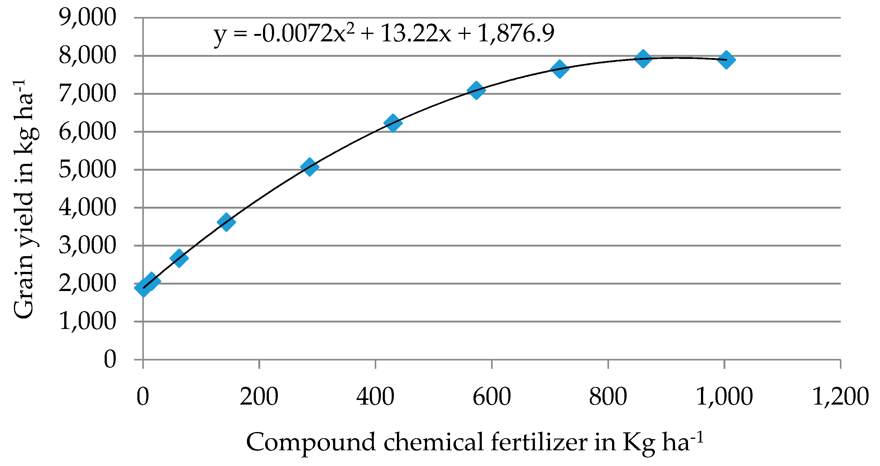
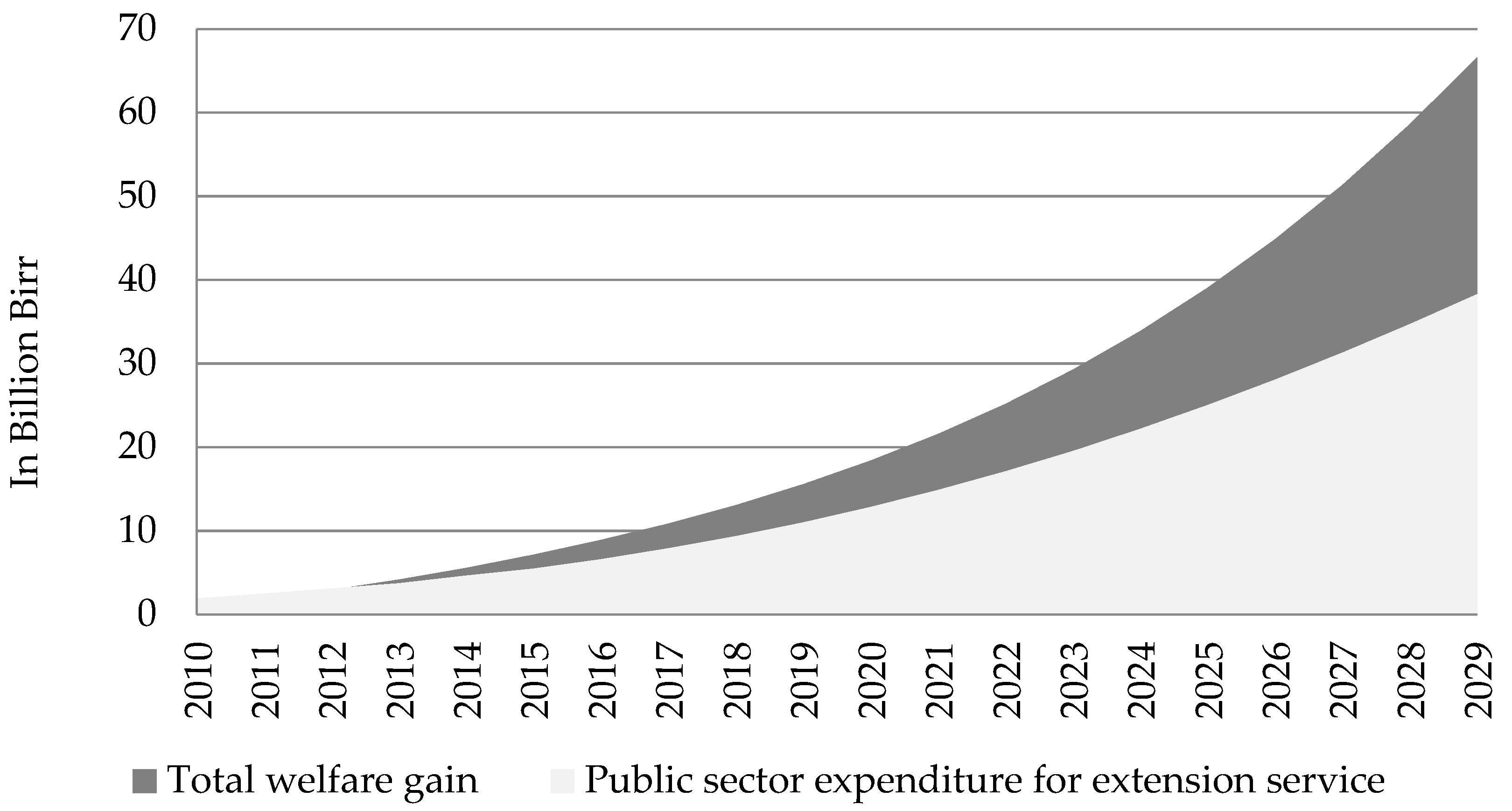
Results show a strong effect of the application rate of mineral fertilizer on maize yield and stover biomass across the AEZs. The national average of maize grain yield under different application rates of the mentioned mix of fertilizers (DAP and urea in a 1:0.9 ratio) is illustrated by Figure 2. The data points allow for a quadratic approximation which is differentiable with respect to fertilizer use and can thus be used to derive economically optimal fertilizer use rates under alternative input and output price constellations. This yields a fertilizer yield response function for maize. (

Table A5. LINTUL5-simulated maize yields, and quadratic approximation function (Ethiopian national average results) at different use levels of mixed fertilizer, and coefficients of the quadratic approximation function.

DAP-Urea Mixed Fertilizer Application in kg/ha	Simulated Yield in kg/ha from LINTUL5	Quadratic Approximation of LINTUL5-Simulated Yields	Deviation
1	1914.24	1890.09	−24.15
62	2687.11	2670.12	−16.99
143	3565.92	3623.61	57.69
287	5024.44	5074.57	50.13
430	6299.13	6229.78	−69.35
573	7153.87	7089.23	−64.64
717	7634.57	7652.93	18.36
860	7848.98	7920.88	71.90
1003	7949.89	7893.07	−56.82

Constant (fertconst): 1876.9; Linear coefficient (fertlin): 13.22; Quadratic coefficient (fertq): −0.0072

displays parameters and results of the quadratic approximation function that is integrated into the CGE model)

The results show that the maximum yield level to be obtained in Ethiopia is far above the current maize yield, which is due to low fertilizer use. At given price levels for fertilizer and maize, the profit function that can be obtained from the yield response function has its optimal fertilizer use level per hectare far above the observed levels. The reason might be unobserved costs in fertilizer use in Ethiopia. Thus, to use this yield function in an economic model, the first order condition (FOC) of the profit function has to be calibrated to current use levels, which is explained in Section 3.3.2.

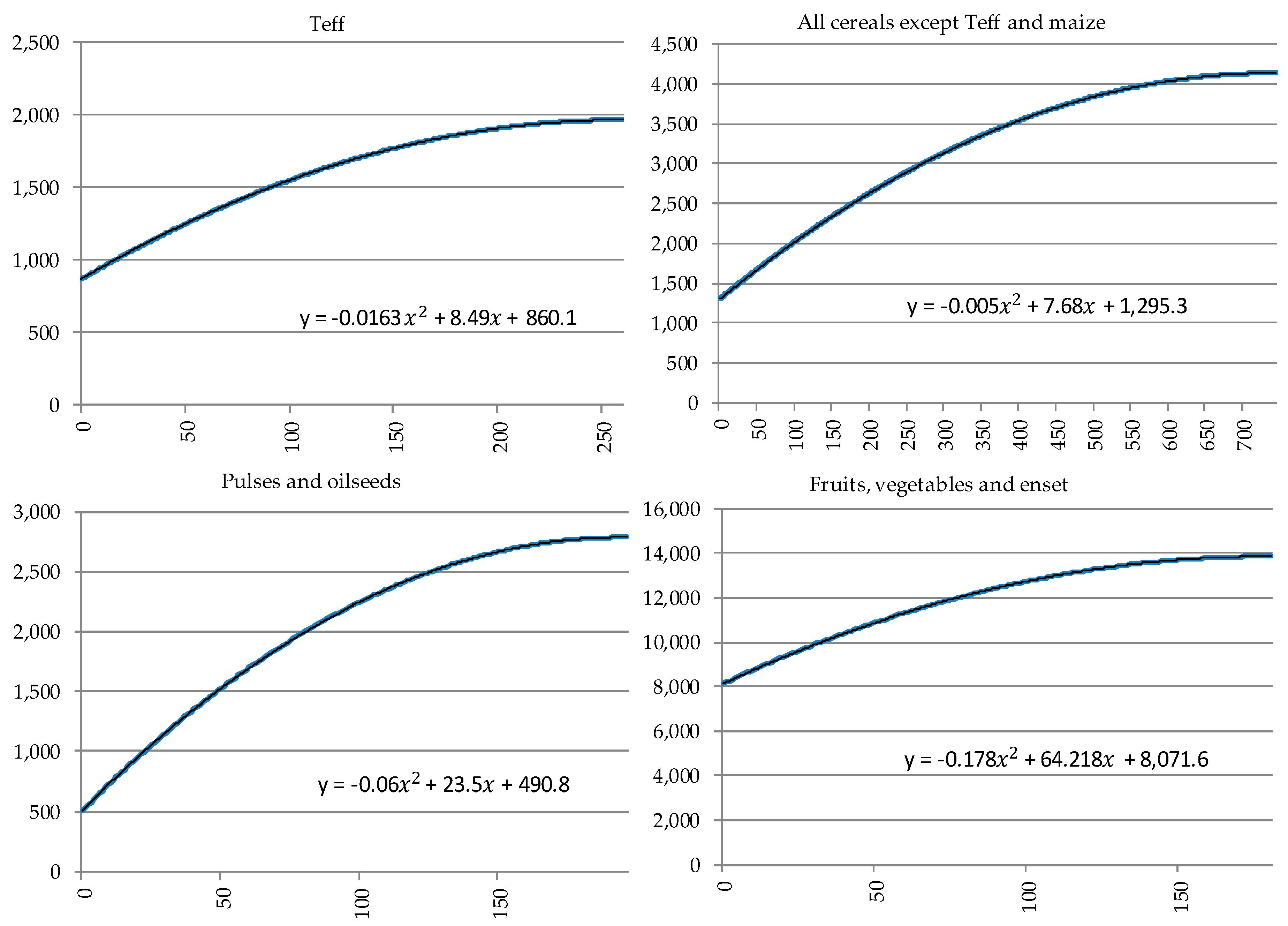
Though we have a crop model only for maize, the other crops in the SAM are considered as well in order to not have maize as the only crop where flexible fertilizer use is linked to productivity. Unlike the estimation strategy applied for maize, actual survey data is used to econometrically estimate fertilizer yield response function for the other crops in the SAM (teff, wheat, barley (Hordeum vulgare), sorghum, pulses, oilseeds, vegetable and fruits, ‘enset’ (false banana), and cash crops like coffee, chat, flower and sugar). We obtain the required data from three rounds (2009/10, 2010/11 and 2011/12) AgSS dataset. Obviously, fertilizer use efficiency of field experiments and actual farmers’ practices cannot be comparable. In order to narrow the gap, we only use farmers that are relatively best in terms of modern agronomic practices – that are under extension coverage and use improved seeds in addition to chemical fertilizer. The fertilizer-yield response function that we estimated for the other crops (i.e., except maize) is displayed in Figure A1. As explained above for maize, at given price levels for the crops and fertilizer, the profit functions that can be obtained from the yield response functions have their optimal fertilizer use levels per hectare far above the observed average levels. These differences exhibit the level of unobserved costs in fertilizer use of the average farmers as compared to the best ones.

3.3.2. Integrating Yield Response into the CGE Model

The principal approach to incorporate a fertilizer yield response function to the CGE model is to create a ‘fertilizer module’, i.e., a set of equations that a) calculates yields, b) identifies optimal fertilizer use levels per hectare based on a profit function approach, and c) finally ensures that changes in nominal quantities and prices obtained in this module are translated into equivalent changes in quantities and prices in the CGE model. Moreover, minor changes to a very limited number of equations of the original CGE model have to be made.

First, the yield (Qyperha_a,c) is defined as a function of fertilizer per hectare by a quadratic model:

$$Qyperh{a}_{a,c}= fert{q}_{a,c} · Qabsfer{t}_{a,c}^2+ fertli{n}_{a,c}· Qabsfer{t}_{a,c}+ fertcons{t}_{a,c}$$

(1)

Where: a stands for set of activities with fertilizer-yield function and c for set of commodities

$fert{q}_{a,c}$ is the quadratic parameter in the yield response function

Qabsfert_a,c is the quantity of fertilizer input per hectare

$fertli{n}_{a,c}$ is the linear parameter in the yield response function

$fertcons{t}_{a,c}$ is the constant term in the yield response function

The parameters of the above quadratic function (fertq_a,c, fertlin_a,c, and fertconst_a,c) are shown in Figure 2 and Figure A1. Now it has to be ensured that changes in output (QA_a) per unit of land use (QF_f,a) in the CGE model compared to its base value are equal to changes of simulated yields per hectare (Qyperha_a,c) relative to its base level (Qyperha0_a,c):

$$\frac{Q{A}_a}{Q{F}_{f,a}}= \frac{QA{0}_a}{QF{0}_{f,a}} ·\frac{Qyperh{a}_{a,c}}{Qyperha{0}_{a,c}}$$

(2)

Where: f stands for set of factors but now specifically represents factor land

$Q{F}_{f,a}$ is a simulated unit of land use

$QF{0}_{f,a}$ is a unit of land use at the base

The next step is defining a fertilizer demand function that expresses marginal revenues and costs of fertilizer use.

Adding prices for the crops and fertilizer (Poutput_a,c and Pfert_c), the profit per hectare of producing commodity c from activity a (π_a,c) can be expressed as:

$${\pi }_{a,c}=Poutpu{t}_c ·Qyperh{a}_{a,c}- Pfer{t}_c· Qabsfer{t}_{a,c}$$

(3)

As yield per hectare (Qyperha_a,c) is a function of fertilizer input per hectare (Qabsfert_a,c), profit per hectare can be re-written by combining Equation 1 and 3. Differentiating it for the decision variable Qabsfert_a,c and solving for the fertilizer price (Pfert_c) yields:

$$Pfer{t}_c= Poutpu{t}_c·\left(2fert{q}_{a,c}·Qabsfer{t}_{a,c}+fertli{n}_{a,c}\right)$$

(4)

The problem is now that if we apply recent average prices (of the crops and fertilizer) in this equation, we would get a much higher fertilizer application rate as observed for Ethiopia. That means there must be unobserved cost elements of fertilizer that were not accounted for, and which we have to add to Pfert_c in order to arrive at observed fertilizer application levels. This fixed calibration factor is thus calculated as the difference between marginal profitability of fertilizer application and marginal fertilizer price. Thus the complete fertilizer demand function is now given as:

$$Pfer{t}_c+fertcali{b}_{a,c}= Poutpu{t}_c· \left(2fert{q}_{a,c}· Qabsfer{t}_{a,c}+fertli{n}_{a,c}\right)$$

(5)

Fertcalib_a,c can be interpreted as an indicator for unobserved costs in fertilizer marketing and use, and could thus be varied in policy simulations or long-term scenarios of better marketing and use efficiency.

We have created a new equation with the first order condition (FOC) above, and we have created two new variables contained in it, the absolute prices for the crop outputs (Poutput_c) and fertilizer (Pfert_c) that have to be defined in related equations. In these, changes in absolute prices are determined by changes in relative prices in the CGE part of the model where markets determine price changes for the crops and fertilizer:

$$\frac{Poutpu{t}_c}{Poutput{0}_c}= \frac{P{Q}_C}{PQ{0}_C}$$

(6)

$$\frac{Pfer{t}_c}{Pfert{0}_c}= \frac{P{Q}_C}{PQ{0}_C}$$

(7)

Where: $P{Q}_C$ is the simulated commodity price in the CGE model

$PQ{0}_C$ is the commodity price in the CGE model at the base

The next step is to enable the CGE model to change its fertilizer input use in accordance with the fertilizer module. By default, single intermediate inputs in the CGE model are a fixed share (ica_c,a) of total intermediate inputs per activity, i.e., a Leontief demand function.

For variable fertilizer use, this restrictive function has to be relaxed and also altered to better reflect crop production processes. First, the ica_c,a input-output coefficients for fertilizer input use are made variable for crops with yield functions while leaving the other inputs’ shares in these crops fixed. Generally, input use in such crops is no longer related to the total quantity of inputs (QINTA_a in the CGE model), but rather to land use, which is the standard way to describe a production technology in agronomy, meaning that

$$QIN{T}_{c,a}=ic{a}_{c,a}·Q{F}_{f,a}$$

(8)

Where: c stands for fertilizer, a for crop activities with fertilizer-yield function, and f for factor land

For these same cropping activities, total input use (QINTA_a) is not a fixed proportion of output anymore but simply the sum of all inputs used (QINT_a,c).

QINTA_a then enters the equation defining total output as a function of factor use (value added) and input use. With a subset of ica_c,a being variable, changes of fertilizer use per unit of land use in the physical fertilizer module can now be translated into input use per unit of land in the CGE model:

$$\frac{ic{a}_{c,a}}{ica{0}_{c,a}}= \frac{Qabsfer{t}_{a,c}}{Qabsfert{0}_{a,c}}$$

(9)

The last necessary step is to relax the fixed ‘yield parameter’ fprd_f,a that is part of the CGE model equation defining value-added creation through factor use. This parameter serves as an equivalent to the yield per hectare from the fertilizer module and therefore has to be made variable for those activity-commodity pairs for which fertilizer yield response function is available. Counterfactual changes in fprd_f,a are then equivalent to changes in crop yields from the yield response functions.

3.4. Simulation Scenarios

Three different scenarios are simulated that run for a period of 20 years from 2011 to 2030: a baseline scenario for reference, and two counterfactual scenarios that simulate decreased costs of fertilizer use and elevated efficiency of application.

Scenario level 1: Baseline scenario (BASE) is the scenario in which relevant trends of the recent past in Ethiopian economy are applied.

The baseline scenario works as a benchmark which aims at continuing recent trends in model drivers over the simulation period. Based on CSA AgSS data for several years, total cropland supply is exogenously made to increase at a decreasing rate as shown in Figure 3. Moreover, based on two rounds of labor force survey data from the CSA 1999 and 2014 [48,49], the supply of agricultural labor (including unskilled labor) is made to increase by 3.19 percent annually while we apply a higher growth rate (6.14 percent) for non-agricultural labor (skilled and semi-skilled).

The other growth drivers in the model are population growth and Total Factor Productivity (TFP). The overall population in the country is made to increase at a decreasing rate for the next 20 years. Using 18 years data (2000–2017) from FAO data portal [50] we calculated and applied the growth trajectory shown in Figure 3 to the model households. The other essential element of economic growth is growth in activities’ TFP. The growth rates applied in the model are calculated in a way that enables the economy to continue growing with the average growth rate reported for the last decade (i.e., 8.6 percent annually). Actual sectoral shares are also considered and growth rates for the other growth drivers are already applied. Thus, on average 5.7, 4.6 and 3.9 percent annual TFP growth rates are applied to agriculture, industry, and service sector activities respectively.

Scenario level 2: Better access to inputs and alternative pace of technological progress

In this scenario there are two simulations: one (F_ACCESS1) which experiments improved fertilizer accessibility through a decline in transaction (including transportation) cost, while the other (F_ACCESS2), on top of this, considers reduced use inefficiency through a reduction in unobserved cost that hinders Ethiopian farmers to optimize fertilizer use. The two simulations are similar to the BASE except for these additional interventions.

As briefly explained in Section 1, infrastructural and institutional predicaments in the country have led to high transaction costs. Referring to Rashid et al. [9], fertilizer transaction (plus transportation) cost to input distribution centers is estimated to be 11 - 23 percent (or 15.3 percent on average) of the landed cost. Additional 5 percent transportation cost is added which is an assumption about the total cost from the distribution center to the farm gate. All these calculations come up with a transaction+transportation cost of 20.3 percent. This is maintained in the SAM first and then it is made to decrease by 5 percent every year for both simulations in the second scenario (

Table 1. Experimental parameters and their respective shocks in the simulations.

Experimental Parameters	Applied on	Annual Change
		BASE	F_ACCESS1	F_ACCESS2
Transaction + transportation cost (percentage of the total value sales)	Fertilizer commodity	-	−5%	−5%
Unobserved transaction cost / use inefficiency (Birr per hectare)	All crop activities	-	-	−1%

). This effectively means around a percent reduction in fertilizer retail price every year. As the price gets cheaper compared to the initial one, the profit maximizing producer is modeled to increase its fertilizer application per hectare. This is well described in the derived fertilizer demand function (see Equation (5) in Section 3.3.2). The optimal level of fertilizer per hectare is then used to calculate total fertilizer physical quantity based on the total area of land for each crop. That gives us the total intermediate demand for fertilizer.

This intervention is with an assumption of a minimum effort by the government to improve the infrastructural and institutional barriers in fertilizer provision which is the public sector’s role towards better input accessibility for the advancement of the agriculture sector.

Moreover, as shown in Table 1, a 1 percent reduction in the unobserved cost (or use inefficiency) is applied every year in F_ACCESS2 simulation on top of the intervention on transaction cost. As explained above in Section 3.3, the profit function obtained from the physical yield function postulates an optimal fertilizer use level per hectare far above the observed (actual) levels. We termed the positive profit, at suboptimal levels of fertilizer use (the parameter fertcalib_a in the CGE model), as unobserved transaction costs or fertilizer use inefficiency. There are different reasons for this far sub-optimal use. The reasons are well explained in the introduction section.

This scenario assumes an achievement of a 1 percent reduction in unobserved cost as a result of public sector’s effort towards addressing the reasons for the observed use inefficiency, for instance through improved access to credit for inputs, facilitating frequent contact with extension agents or provision of any other knowledge dissemination mechanisms that can improve farmers access to and understanding of modern inputs. Obviously, this intervention would have, in absolute terms, different level of effects for different crop types based on the difference in the initial level of unobserved cost ($fertcali{b}_{a,c}$). Those crops with bigger initial unobserved cost would benefit bigger from a percent reduction in unobserved cost applied on all crops.

The above mentioned interventions to improve the agriculture sector in Ethiopia need significant investment, especially from the government side. Even though we do not have the intention to do a thorough analysis on the cost-benefit comparison at the national level in this paper, it is worthwhile to mention quotes on the required public expenditure in order to undertake such interventions and attain the intended progress in the agriculture sector. Moreover, we also calculate the extent to which the possible benefits could cover the intended expenditure. According to the estimation in the Comprehensive Africa Agriculture Development Programme (CAADP) framework, an allocation of at least 10 percent of public expenditure to the agriculture sector is needed for the overall rural and agricultural development envisioned in Africa [51]. Specifically, if we take agriculture extension service in Ethiopia; it has traditionally been financed and provided almost entirely by the public sector. Thus, these programs represent a significant public investment, roughly estimated to be 2 percent of total annual government expenditure [52].

4. Results and Discussion

As explained above, the interventions in this modeling work are applied to a number of crops. Discussing the results of each of these is time consuming and less important. Hence, we present results on the overall crops in general, and teff and maize in particular as they are the two most important crops in Ethiopia. Teff and maize hold the 1^st and 2^nd place in terms of crop output and land coverage. From consumption side, teff is mainly used for making ‘enjera’, the main national dish in Ethiopia (as well as Eritrea). Regarding maize, since it is the cheapest cereal crop, the poor (especially the rural poor) consume it mostly. It’s crucial for national food security.

4.1. Supply (production) Effects and Economic Growth

Let us start the analysis with model results on food supply as the counterfactual scenarios are designed to improve productivity in crop production. The reduction in transaction (plus transportation) cost leads to an average of 0.5 percentage points annual decline in fertilizer retail price compared to the base line situation. This intervention together with the decline in unobserved costs increases the use of fertilizer. As a result, the experimental simulations show a positive response in yields and total output.

As shown in

Table 2. Average annual chemical fertilizer application and yield level (kg per hectare).

	BASE		F_ACCESS1		F_ACCESS2
	DAP+urea	Output	DAP+urea	Output	DAP+urea	Output
Teff	38.0	1162.7	40.1	1177.2	50.6	1246.1
Maize	116.0	3284.1	122.0	3350.1	149.7	3641.6
All crops	56.8	2156.7	61.5	2194.9	76.3	2344.3

, a 5 percent annual reduction in transaction costs on fertilizer acquisition (i.e., F_ACCESS1) motivates higher fertilizer application. In the BASE run, an average Ethiopian crop farmer applies 56.8 kg of chemical fertilizer on a hectare plot which would rise to 61.5 kg as a result of the intervention. The improved soil fertility, consequently, would give an average 2.2 tons (i.e., additional yield of about 38.2 kg) per hectare crop each year. Looking at individual crops, the intervention encourages teff and maize farmers increase their fertilizer application rate at the BASE (i.e., 38 and 116 kg per hectare respectively) to 40.1 and 122.0 kg per hectare. As a result teff and maize farmers’ yield levels rise by 1.2 and 2.0 percent of the BASE and reach 1.18 and 3.35 tons per hectare.

On the other hand, if unobserved costs in fertilizer use could be reduced by 1 percent every year (i.e., F_ACCESS2), then the average farmer would annually apply 76.3 kg chemical fertilizer per hectare (i.e., additional of 34.2 percent of the BASE), which would lead to 8.7 percent increase in yield level per hectare. Teff and maize farmers would gain higher yield levels; 1.3 and 3.6 tons, which are higher than the BASE by 7.2 and 10.9 percent as a result of application of additional 12.5 and 33.7 kg fertilizer per hectare on teff and maize plots respectively.

Based on this achievement in yield and the resulted factor re-distribution in the model, the country’s total crop production per annum would increase in F_ACCESS1 and F_ACCESS2 by 1.9 and 7.7 percent higher than it increases in the current growth trend (i.e., BASE). This implies a 0.8 and 3.2 million tons of annual crop supply additional to the current achievement level. In teff and maize production F_ACCESS2 would come up with the maximum effect - an additional of 5.7 and 5.5 percent of the current annual production level per annum, respectively. This means around 377 and 385 thousand metric tons of teff and maize.

Looking at the dynamics, yields of all crops, including teff and maize, increase at a decreasing rate. Even though this trend holds for all the simulations, both counterfactual scenarios, especially F_ACCESS2 results in significantly stronger effects on the yield trend. As seen in Figure 4, the differential between the BASE and the counterfactual simulations is increasing throughout the period for all crops. The cumulated effects of the introduced shocks in both simulations make the activities produce consecutively higher amounts of output on a given plot. Crop yield grows by about 40 kg ha⁻¹ on average per annum because of increased fertilizer use as a result of decreased acquisition cost (i.e., F_ACCESS1). Improving fertilizer accessibility and use efficiency simultaneously (i.e., F_ACCESS2) obtains the highest productivity gain for all crops: yield increases on average by about 197 kg ha⁻¹. The dynamics in both fertilizer application and yield gain show that reducing the inefficiency for modern input use is highly critical and makes the effort to improve input adoption even more effective.

One benefit of the productivity improvements in domestic crop production might be a reduced import dependency of food staples. For instance, due to frequent droughts (especially in the drought-prone areas of east and south-east parts of Ethiopia) and rising food prices, the government of Ethiopia relies on wheat imports for relief and market stabilization. Thus, according to FAOSTAT [50], Ethiopia’s wheat imports increased more than three-fold in the last twenty-five years. For instance, from 2008-2013 the country imported an average of about half a billion USD worth of wheat each year, putting a burden on Ethiopia’s foreign currency reserve. The additional output obtained as a result of the simulated interventions could contribute to easing this deficit by boosting domestic production of staple grains. Annual wheat import would reduce as a result of the counterfactual interventions by 8.7 percent of the current annual import volume which means the country could save a maximum of a quarter of its import from 2008–2013. Moreover, looking at the country’s import of crop commodities, the baseline interventions would increase import demand for all the simulations. However, the counterfactual interventions would reduce crop imports by 3 and 9 percent of the baseline performance annually. Regarding fertilizer import, as both the counterfactual interventions would significantly boost the demand for fertilizer, it would directly be reflected on the country’s import bill. Fertilizer import would annually increase in F_ACCESS1 and F_ACCESS2 by 7.7 and 32 percent of the current annual import level.

The interventions introduced in the farming sector have a strong impact on macroeconomic aggregates as well. Aggregate value added is significantly increasing for all the simulations. However, when comparing to the BASE, as can be seen from Figure 5, the additional GDP obtained as a result of the counter factual interventions increases at an increasing rate consecutively. The effect gets stronger when efficiency is improved in fertilizer use together with a higher application rate. The fact that all the counter factual interventions are applied on the crop sub-sector, which contributes around 32 percent of the total GDP, makes interventions with strong implications on this sub-sector strongly reflect on the national GDP. However, the weak linkage between the agriculture and non-agriculture sectors (well discussed in Section 3.2) significantly reduces the implication of agriculture growth to the non-agriculture economy. For instance, following the interventions in F_ACCESS2, crop sub-sector GDP increases by 2 percentage points with the agriculture GDP increasing by 1.4 percentage points, while the non-agriculture GDP rises by only 0.01 percentage points in comparison with the BASE. Moreover, the fact that the country is not exporting most of the crops that receive the interventions, the success obtained in increasing production brings only 0.03 and 0.09 percentage points increase in volume of export. Thus, almost the entire additional production is sold to the domestic market that implies decreasing crop prices that fall on average by 0.33 percentage points in comparison with the BASE. This has adverse effect on (net food seller) farmers’ income.

4.2. Effects on Household Income

All the simulations bring about significantly increasing income changes for both farming and non-farming households. However, compared to the BASE scenario, the additional productivity gain resulting from the two counterfactual simulations leads to a small impact on income for both household types. As highlighted above, the shocks involved in the two counterfactual simulations relatively decrease crop prices, which have an adverse effect on the income of net seller farming households. Moreover, as shown in Table A4 in the annex, non-farming households basically receive most of their income from skilled labor and capital employment in the non-agriculture sector which is marginally affected by the relevant interventions. If we look at the households by their income classification, F_ACCESS1 and F_ACCESS2 enable poor farmers to obtain incomes that are 0.07 and 0.25 percentage points higher, respectively, as compared to the BASE. Non-poor farming households receive 0.06 and 0.26 percentage points higher incomes. Non-farming households similarly enjoy a slight increase in income of 0.04 percentage points as a result of F_ACCESS1 and 0.25 and 0.26 percentage points for the poor and non-poor counter parts respectively as a result of F_ACCESS2.Looking at the aggregate effect doesn’t show us the impact on the specific household, so that effects on the profitability of crop farming in particular need to be discussed. It is possible to calculate income effects through profitability of the additional fertilizer applied. A commonly used measure of profitability is the value-cost ratio (VCR) (Equation 10). Here it is applied to the model results (i.e., additional chemical fertilizer used per holder and the additional output obtained as a result - both in kg to calculate the profitability of additional fertilizer used per holder’s plot relative to BASE). This ratio is the value of the additional production due to application of the additional fertilizer to the total cost of the additional fertilizer applied. The additional output from an average crop plot that received the additional fertilizer is X. P is the price of crop output (farm gate price). Price of fertilizer is P_f, and Q_f is the additional amount of fertilizer applied to that particular plot, then the VCR is given as follows:

$$VCR=\frac{P\times X}{P_f\times Q_f }$$

(10)

Looking at the results from

Table 3. VCR calculations for additional fertilizer application on an average Ethiopian crop farming plot.

Fertilizer price Birr per kg	F_ACCESS1			F_ACCESS2
	14.76			14.76
Teff price Birr per kg	7.10			7.09
Maize price Birr per kg	2.94			2.94
All crops average price Birr per kg	4.00			4.00
	Teff	Maize	All crops	Teff	Maize	All crops
Additional DAP+urea used per holder (kg)	0.96	1.49	1.02	5.76	8.35	4.26
Additional output (kg)	6.63	16.38	8.38	38.30	88.64	41.15
Additional spending for fertilizer (birr)	14.18	21.94	15.09	85.08	123.22	62.94
Additional birr obtained from sales	47.08	48.17	33.55	271.52	260.27	291.70
Additional profit in birr	32.89	26.24	18.46	186.44	137.05	228.76
VCR	3.32	2.20	2.22	3.19	2.11	4.63

Note: All the acreage and price figures basically used in this calculation are subject to changes from the model results.

, the VCR levels mean that each kg of additional fertilizer applied on the crop plots is found to be highly profitable to the holder. As can be understood from the formula, a VCR of 1 is the threshold to profitability. However, it is commonly argued that a VCR of at least 2 is needed for fertilizer to be profitable in Africa. A high threshold level is recommended for Africa just to compensate for the higher probability of adverse conditions that greatly influence profitability, as for instance infestations and weather risks [9].

An average teff farmer in Ethiopia with a 0. 460 ha plot obtains an additional 32.9 and 186.4 Birr profit from applying an additional 1 and 5.76 kg of chemical fertilizer in F_ACCESS1 and F_ACCESS2, respectively. Similarly, an average maize farmer gets from 26.2 to 137 Birr profit from his quarter of a hectare plot as a result of the application of additional 1.5 to 8.4 kg chemical fertilizer in the two simulations. Looking at the overall crop sub-sector, an average crop farmer with 0.219 ha plot enjoys 18.5 and 228.8 Birr profit applying an additional 1 and 4.3 kg chemical fertilizer. As discussed above, the VCR levels from Table 3 show that each Birr spent to purchase additional fertilizer for teff and maize in particular and all crops production in general are very profitable. These results indicate that improved fertilizer accessibility and reduced use inefficiency could make a significant difference regarding fertilizer application and profitability. Thus, as compared to BASE, crop farmers are better off in terms of profitability. This positive effect could be higher with greater fertilizer application.

In an attempt to look at the welfare gains and losses to market participants from changes in market conditions as a result of the interventions, aggregate value added is calculated for each intervention. Let us take the last intervention (for the sake of a straight forward calculation of its budgetary cost) and assume the 1 percent annual reduction in unobserved cost for crop farmers is attainable through improved access to better quality extension service. As a result, this intervention would result in a total welfare gain of about 66.6 billion Birr in the country in 2030 which grows from 0.8 billion Birr in 2011 with a 27.5 percent average annual growth rate. Based on data from National Bank of Ethiopia NBE [53] and estimation by Spielman et al. [52] average annual total public expenditure on extension service is calculated to be 3.65 billion Birr between 2009/10 and 2016/17. We also made a projection until 2030 based on recent years’ growth trend. The current and projected public expenditure on extension service is then calculated to be 82 percent of the expected welfare gain obtained from increased efficient fertilizer use as a result of improved provision of extension service. (See Figure 6) The welfare gain is encouraging and could sufficiently cover expenditure to further improve the agriculture extension service.

4.3. Effects on Household Consumption

When discussing changes in household welfare as a result of productivity interventions, a distinction between net producers and net consumers of crops has to be made. Subsequent price drops have adverse effects on net producers, whereas they are benefits to net consumers. A broader perspective is needed to deal with this issue, as households have diverse sources of income and lower crop prices even could have positive effects on the producer households’ consumption expenditure. Income improvements (see Section 4.2) and price reductions are obtained from the model results. Average crop price annually decreases at a maximum of 0.03 and 0.28 percentage points relative to the BASE in F_ACCESS1 and F_ACCESS2, respectively. Thus, households that are highly dependent on these commodities, such as rural farming households which consume 35 percent of their total consumption from crop commodities, would exhibit higher welfare improvements as a result of cheaper consumption than households that consume less of these commodities (in our case, non-farming households whose consumption bundle comprises of only 15 percent crop commodities). Referring to Figure 7, farming households enjoy higher consumption increases in the experimental simulations than non-farming households. The price decrease under F_ACCESS2 enables farming households to enjoy a higher welfare gain than net consumers even though both enjoy an equal rise in income. However, price and income changes work together to make all household categories better-off as a result of the counter factual interventions. Non-farming households’ welfare improves as well as a result of reduced cost of living and rise in income.

5. Conclusions

The overarching objective of this study was to examine the economy-wide implications of improved access to and use efficiency of modern farming inputs, particularly fertilizer with a major emphasis on the resulting household welfare. The study is motivated by the situation in Ethiopia in which cropland scarcity is bound to be a serious challenge for the future growth in food supply. Using a dynamic CGE model for Ethiopia and estimated fertilizer-yield response functions we investigate macro and micro effects of improved fertilizer application.

In comparison with current trends, model results show positive effects in the two experimental simulation scenarios: 1. reduction in fertilizer transaction costs to make fertilizer more accessible, and 2. annual reduction in unobserved transaction cost of fertilizer use, on top of the first one, as a result of the public sector’s effort to address the reasons for fertilizer use inefficiency. Both experimental simulations are applied to all crops. In both simulations, the interventions would come up with a significant increase in yields and total output both at the aggregate and household level. Based on the importance of cereals in the national food basket, 46.3 percent according to Brhane et al. 2011 [54], this significant improvement in total domestic production has huge impacts on the national food security and stabilizing the domestic cereal market. It could also ease the country’s BoP deficient that is currently worsening as a result of increased food and fertilizer imports, among others. The results also suggest that the increased fertilizer application is highly profitable for an average crop farmer with 0.219 hectare plot. If the entirety of households in the economy is considered, effects of the new interventions on crop price and household income together enables them to enjoy higher welfare, especially farming households when higher fertilizer amount is applied efficiently. This is especially meaningful for the farming population in Ethiopia, who frequently experience food insecurity.

Moreover, the aggregate welfare effect indicates that these interventions are profitable in general. Assuming a reduction in fertilizer use inefficiency attainable through improved access to extension services, the total welfare gain that would be achieved is found to be equivalent to 135 percent of the current annual public expenditure on extension service. Putting this into perspective, we can see how economically viable the intended intervention is. The welfare gain from the intervention on the crop sub-sector could sufficiently justify complete financing of the total cost with extra money that can finance an increase of 35 percent of the entire current public expenditure on farm extension services.

Thus, in order to reap these potential benefits, reductions in transaction costs of fertilizer acquisition could be achieved in different ways. Improving the rural road network would reduce the cost markup from harbor to farm. Additionally, reducing bureaucratic obstacles in fertilizer procurement could avoid belated input application, which decreases the use inefficiency. Finally, improved accessibility to agriculture extension agents and creating possible alternative income sources, especially off-farm, would significantly ease adoption barriers and cut the high knowledge costs related to the adoption of new technologies. The comparison between the two counterfactual simulations shows that improved efficiency regarding modern input use is highly critical and makes the effort to improve input adoption even more effective.

Though the interventions have strong positive effects on the economy, increased fertilizer import has adverse effect on the country’s balance of payment (BoP). Moreover, the fact that most of the crops that enjoy the interventions are non-tradables, the increased production ends up in domestic price decrease which has adverse effect on net seller farmers’ income. Thus, as a policy recommendation, if Ethiopia introduces most of its crops to the export market, it could be of double advantage; 1. It could serve the BoP deficit resulting from increases in fertilizer import, and 2. It provides the farmers with an opportunity to get better price.

Policy makers should focus on strengthening the agriculture – industry linkage in order to make growth in the agriculture sector transmit and trigger growth in the non-agriculture sector. The possible pathways are 1. Through commencement of domestic fertilizer production and supply which is advantageous for faster and timely distribution, lower price provision and easing BoP burden of fertilizer imports. 2. Through promoting expansion of the food processing industry sub-sector. As the urban centers in Ethiopia get more and more populous and modernized, the demand for ready-made (or packed) foods is increasing. There are few industries operating at micro and small scale trying to satisfy this demand. Policy focus on these kinds of industries could benefit the economy with strong linkage between the agriculture and non-agriculture sector and households with cheaper costs of living.

References

1. Boserup, E. The Conditions of Agricultural Growth: The Economics of Agrarian Change under Population Pressure; G. Allen and Unwin LTD: London, UK, 1965; pp. 104–105. [Google Scholar]
2. Demeke, M.; Kelly, V.; Jayne, T.S.; Said, A.; Le Vallee, J.C.; Chen, H. Agricultural Market Performance and Determinants of Fertilizer Use in Ethiopia. Grain Market Research Project; Working Paper No.10; Ministry of Economic Development and Cooperation: Addis Ababa, Ethiopia, 1998. [Google Scholar]
3. World Bank. Ethiopia Poverty Assessment 2014. Poverty Global Practice Africa Region. Report No. AUS6744. Available online: http://documents.worldbank.org/curated/en/131011468247457565/pdf/AUS67440REVISE0sessment0pub02020015.pdf (accessed on 3 March 2019).
4. Kassie, M.; Shiferaw, B.; Muricho, G. Agricultural Technology, Crop Income, and Poverty Alleviation in Uganda. World Dev. 2011, 39, 1784–1795. [Google Scholar] [CrossRef]
5. Becerril, J.; Abdulai, A. The impact of improved maize varieties on poverty in Mexico: A propensity score matching approach. World Dev. 2010, 38, 1024–1035. [Google Scholar] [CrossRef]
6. Duflo, E.; Kremer, M.; Robinson, J. How High are Rates of Return to Fertilizer? Experimental Evidence from Kenya. Am. Econ. Rev. 2008, 98, 482–488. [Google Scholar] [CrossRef]
7. Minten, B.; Barrett, C.B. Agricultural technology, productivity, and poverty in Madagascar. World Dev. 2008, 36, 797–822. [Google Scholar] [CrossRef]
8. Jayne, T.S.; Chamberlin, J.; Headey, D.D. Land Pressures, the Evolution of Farming Systems, and Development Strategies in Africa: A Synthesis. Food Policy 2014, 48, 1–17. [Google Scholar] [CrossRef]
9. Rashid, S.; Tefera, N.; Minot, N.; Ayele, G. Fertilizer in Ethiopia: An Assesment of Policies, Value Chain, and Profitability; Discussion Paper 1304; International Food Policy Research Institute: Washington, DC, USA, 2013. [Google Scholar]
10. Zerfu, D.; Larson, D. Incomplete Market and Fertilizer Use: Evidence from Ethiopia; Policy Research Working Paper, WPS5235; World Bank: Washington, DC, USA, 2010. [Google Scholar]
11. Minten, B.; Koru, B.; Stifel, D. The Last Mile(s) in Modern Input Distribution: Pricing, Profitability, and Adoption. Agric. Econ. 2013, 44, 629–646. [Google Scholar] [CrossRef]
12. Yu, B.; Nin-Pratt, A.; Funes, J.; Asrat, S. Cereal Production and Technology Adoption in Ethiopia. In Proceedings of the 8th International Conference of the Ethiopian Economic Association, Addis Ababa, Ethiopia, 25 June 2010. [Google Scholar]
13. Asrat, S.; Bizuneh, G.; Taffesse, A.S. Trends and Determinants of Cereal Productivity in Ethiopia. In Proceedings of the 8th International Conference of the Ethiopia Economic Association, Addis Ababa, Ethiopia, 22 June 2010. [Google Scholar]
14. Nisrane, F.; Berhane, G.; Asrat, S.; Bizuneh, G.; Taffesse, A.S.; Hoddinott, J. Sources of Inefficency and Growth in Agricultural Output in Subsistence Agriculture: A Stochastic Frontier Analysis; ESSP2 Working Paper 19; International Food Policy Research Institute: Washington, DC, USA, 2011. [Google Scholar]
15. Dorward, A.; Chirwa, E. The Malawi agricultural input subsidy programme: 2005/06 to 2008/09. Int. J. Agric. Sustain. 2011, 9, 232–247. [Google Scholar] [CrossRef] [Green Version]
16. Bold, T.; Kaizzi, K.; Svensson, J.; Yanagizawa-Drott, D. Low Quality, Low Returns, Low Adoption: Evidence from the Market for Fertilizer and Hybrid Seed in Uganda; Working Paper Series rwp15-033; Harvard University, John F. Kennedy School of Government: Cambridge, MA, USA, 2015. [Google Scholar]
17. Yu, B.; Nin-Pratt, A. Fertilizer Adoption in Ethiopia Cereal Production. J. Dev. Agric. Econ. 2014, 6, 318–337. [Google Scholar] [CrossRef]
18. Beshir, H.; Emana, B.; Kassa, B.; Haji, J. Determinants of Chemical Fertilizer technology Adoption in North Eastern Highlands of Ethiopia: The Double Hurdle Approach. J. Res. Econ. Int. Financ. 2012, 1, 39–49. [Google Scholar]
19. Verkaart, S.; Munyua, B.G.; Mausch, K.; Michler, J.D. Welfare Impacts of Improved Chickpea Adoption: A Pathway for rural Development in Ethiopia? Food Policy 2017, 66, 50–61. [Google Scholar] [CrossRef] [PubMed]
20. Caria, A.S.; Tamiru, S.; Bizuneh, G. Food Security Without Food Transfers? A CGE Analysis for Ethiopia of the Different Food Security Impacts of Fertilizer Subsides and Locally Sourced Food Transfers; IFPRI Discussion Paper 01106; International Food Policy Research Institute: Washington, DC, USA, 2011. [Google Scholar]
21. Arndt, C.; Pauw, K.; Thurlow, J. The Economy-Wide Impacts and Risks of Malawi’s Farm Input Subsidy Program. Am. J. Agric. Econ. 2016, 98, 962–980. [Google Scholar] [CrossRef]
22. Bachewe, F.N.; Berhane, G.; Minten, B.; Taffesse, A.S. Agricultural Growth in Ethiopia (2004–2014): Evidence and Drivers; ESSP Working Paper 81; International Food Policy Research Institute: Washington, DC, USA, 2015. [Google Scholar]
23. Martins, P. Structural Change in Ethiopia: An Employment Perspective; Policy Research Working Paper, WPS 6749; World Bank: Washington, DC, USA, 2014. [Google Scholar]
24. National Bank of Ethiopia (NBE). Annual Report 2013/2014. Annual Report. 2014. Available online: http://www.nbe.gov.et/pdf/annualbulletin/Annual%20Report%202013-2014/Annex%202013-14newst.pdf (accessed on 25 November 2017).
25. Central Statistics Agency (CSA). Agriculture Sample Survey 2015/16 (2008 E.C.). Statistical Bulletin, Report on Area and Production of Major Crops (Private Peasant Holdings, Meher Season); CSA: Addis Ababa, Ethiopia, 2016.
26. Central Statistics Authority (CSA). Agriculture Sample Survey 2004/05 (1997 E.C.). Statistical Bulletin, Report on Area and Production of Major Crops (Private Peasant Holdings, Meher Season); CSA: Addis Ababa, Ethiopia, 2005.
27. Central Statistics Agency (CSA). Agriculture Sample Survey 2005/06 (1998 E.C.). Statistical Bulletin, Report on Area and Production of Major Crops (Private Peasant Holdings, Meher Season); CSA: Addis Ababa, Ethiopia, 2006.
28. Central Statistics Agency (CSA). Agriculture Sample Survey 2006/07 (1999 E.C.). Statistical Bulletin, Report on Area and Production of Major Crops (Private Peasant Holdings, Meher Season); CSA: Addis Ababa, Ethiopia, 2007.
29. Central Statistics Agency (CSA). Agriculture Sample Survey 2007/08 (2000 E.C.). Statistical Bulletin, Report on Area and Production of Major Crops (Private Peasant Holdings, Meher Season); CSA: Addis Ababa, Ethiopia, 2008.
30. Central Statistics Agency (CSA). Agriculture Sample Survey 2008/09 (2001 E.C.). Statistical Bulletin, Report on Area and Production of Major Crops (Private Peasant Holdings, Meher Season); CSA: Addis Ababa, Ethiopia, 2009.
31. Central Statistics Agency (CSA). Agriculture Sample Survey 2009/10 (2002 E.C.). Statistical Bulletin, Report on Area and Production of Major Crops (Private Peasant Holdings, Meher Season); CSA: Addis Ababa, Ethiopia, 2010.
32. Central Statistics Agency (CSA). Agriculture Sample Survey 2010/11 (2003 E.C.). Statistical Bulletin, Report on Area and Production of Major Crops (Private Peasant Holdings, Meher Season); CSA: Addis Ababa, Ethiopia, 2011.
33. Central Statistics Agency (CSA). Agriculture Sample Survey 2011/12 (2004 E.C.). Statistical Bulletin, Report on Area and Production of Major Crops (Private Peasant Holdings, Meher Season); CSA: Addis Ababa, Ethiopia, 2012.
34. Central Statistics Agency (CSA). Agriculture Sample Survey 2012/13 (2005 E.C.). Statistical Bulletin, Report on Area and Production of Major Crops (Private Peasant Holdings, Meher Season); CSA: Addis Ababa, Ethiopia, 2013.
35. Central Statistics Agency (CSA). Agriculture Sample Survey 2013/14 (2006 E.C.). Statistical Bulletin, Report on Area and Production of Major Crops (Private Peasant Holdings, Meher Season); CSA: Addis Ababa, Ethiopia, 2014.
36. Central Statistics Agency (CSA). Agriculture Sample Survey 2014/15 (2007 E.C.). Statistical Bulletin, Report on Area and Production of Major Crops (Private Peasant Holdings, Meher Season); CSA: Addis Ababa, Ethiopia, 2015.
37. World Bank. Background Report: Four Ethiopias, A Regional Characterization; Assessing Ethiopia’s Growth Potential and Development Obstacles. Economic Memorandum; World Bank: Addis Ababa, Ethiopia, 2004. [Google Scholar]
38. Central Statistical Authority (CSA). Agricultural Sample Survey 2003/2004 (1996 E.C.). Statistical Bulletin, Report on Area and Production of Major Crops (Private Peasant Holdings, Meher Season); CSA: Addis Ababa, Ethiopia, 2004.
39. UNDP. Human Development Reports 2017. Available online: http://hdr.undp.org/en/composite/HDI (accessed on 15 March 2019).
40. Lofgren, H.; Harris, R.L.; Robinson, S. A Standard Computable General Equilibrium (CGE) Model in GAMS; Discussion Paper 75; International Food Policy Research Institute, Trade and Macroeconomics Division: Washington, DC, USA, 2001. [Google Scholar]
41. Dorosh, P.; Thurlow, J. Implications of Accelerated Agricultural Growth on Household Incomes and Poverty in Ethiopia: A General Equilibrium Analysis. ESSP2 Working Paper 002. Available online: http://ebrary.ifpri.org/utils/getfile/collection/p15738coll2/id/130942/filename/131153.pdf (accessed on 4 May 2019).
42. Engida, E.; Tamru, S.; Tsehaye, E.; Debowicz, D.; Dorosh, P.A.; Robinson, S. Ethiopia’s Growth and Transformation Plan: A Computable General Equilibrium Analysis of Alternative Financing Options; ESSP Working Paper 30; International Food Policy Research Institute: Washington, DC, USA, 2011. [Google Scholar]
43. Gaiser, T.; Perkons, U.; Küpper, P.M.; Kautz, T.; Uteau-Puschmann, D.; Ewert, F.; Enders, A.; Krauss, G. Modeling biopore effects on root growth and biomass production on soils with pronounced sub-soil clay accumulation. Ecol. Model. 2013, 256, 6–15. [Google Scholar] [CrossRef]
44. Addiscott, T.M.; Whitmore, A.P. Simulation of solute leaching in soils of differing permeabilities. Soil Use Manag. 1991, 7, 94–102. [Google Scholar] [CrossRef]
45. Jaleta, M.; Kassie, M.; Shiferaw, B. Tradeoffs in crop residue utilization in mixed crop–livestock systems and implications for conservation agriculture. Agric. Syst. 2013, 121, 96–105. [Google Scholar] [CrossRef]
46. Srivastava, A.K.; Mboh, C.M.; Gaiser, T.; Zhao, G.; Ewert, F. Climate change impact under alternate realizations of climate scenarios on maize yield and biomass in Ghana. Agric. Syst. 2018, 159, 157–174. [Google Scholar] [CrossRef]
47. Srivastava, A.; Gaiser, T.; Ewert, F.; Mboh, C.M.; Engida, E.; Kuhn, A. Effect of Mineral Fertilizer on Rain Water and Radiation use Efficiencies for Maize Yield and Stover Biomass Productivity in Ethiopia. Agric. Syst. 2019, 168, 88–100. [Google Scholar] [CrossRef]
48. Central Statistics Authority (CSA). Statistical Report on The 1999 National Labour Force Survey; Statistical Bulletin No. 225; CSA: Addis Ababa, Ethiopia, 1999.
49. Central Statistical Agency (CSA). Analytical Report on The 2013 National Labour Force Survey; Statistical Bulletin; CSA: Addis Ababa, Ethiopia, 2014.
50. Food and Agriculture Organization (FAO). FAOSTAT. Available online: http://www.fao.org/faostat/en/#country/238 (accessed on 4 December 2017).
51. New Partnership for Africa’s Development (NEPAD). Comprehensive Africa Agriculture Development Programme; New Partnership for Africa’s Development (NEPAD): Midrand, South Africa, 2003; ISBN 0-620-30700-5. [Google Scholar]
52. Spielman, D.J.; Mekonnen, D.K.; Alemu, D. Seed, Fertilizer, and Agriculture Extension in Ethiopia. In Food and Agriculture in Ethiopia: Progress and Policy Challenges; Poul, D.A., Rashid, S., Eds.; University of Pennsylvania Press: Philadelphia, PA, USA, 2012; pp. 84–122. ISBN 9780812245295. [Google Scholar] [CrossRef]
53. National Bank of Ethiopia (NBE). 2016/17 Annual Report. Available online: http://www.nbe.gov.et/pdf/annualbulletin/NBE%20Annual%20report%202016-2017/NBE%20Annual%20Report%202016-2017.pdf (accessed on 3 September 2018).
54. Berhane, G.; Paulos, Z.; Tafere, K.; Tamiru, S. Foodgrain Consumption and Clorie Intake Patterns in Ethiopia; ESSP 2. Working Paper 23; International Food Policy Research Institute: Washington, DC, USA, 2011. [Google Scholar]
Figure 1. Trend in fertilizer application (2003/04 – 2015/16).
Sustainability 11 03952 g001
Figure 2. LINTUL5-simulated maize yields, and quadratic approximation function (Ethiopian national average results) at different use levels of mixed chemical fertilizer.
Sustainability 11 03952 g002
Figure 3. Land and population growth trends (2011-2030).
Sustainability 11 03952 g003
Figure 4. Dynamics in yield (2010-2030) (deviations between BASE and experimental simulation trajectories) for a) teff and maize and b) all crops.
Sustainability 11 03952 g004
Figure 5. Dynamics in the aggregate value addition (2010-2030), comparison with the BASE (in billion birr).
Sustainability 11 03952 g005
Figure 6. Trajectories for public expenditure on extension service and the expected total welfare gain.
Sustainability 11 03952 g006
Figure 7. Dynamics in simulation results on households’ consumption (2010-2030) (percentage deviation between BASE and simulation trajectories).
Sustainability 11 03952 g007