Predicting Safe Parking Spaces: A Machine Learning Approach to Geospatial Urban and Crime Data

1
Data Science Institute, Saint Peter’s University, Jersey City, NJ 07306, USA
2
Centre for Smart Cities and Infrastructure, Kaunas University of Technology, Kaunas 44249, Lithuania
3
Amazon Robotics, Boston, MA 01864, USA
*
Author to whom correspondence should be addressed.
Sustainability 2019, 11(10), 2848; https://doi.org/10.3390/su11102848
Submission received: 11 April 2019
/
Revised: 13 May 2019
/
Accepted: 13 May 2019
/
Published: 19 May 2019
Abstract
:This research aims to identify spatial and time patterns of theft in Manhattan, NY, to reveal urban factors that contribute to thefts from motor vehicles and to build a prediction model for thefts. Methods include time series and hot spot analysis, linear regression, elastic-net, Support vector machines SVM with radial and linear kernels, decision tree, bagged CART, random forest, and stochastic gradient boosting. Machine learning methods reveal that linear models perform better on our data (linear regression, elastic-net), specifying that a higher number of subway entrances, graffiti, and restaurants on streets contribute to higher theft rates from motor vehicles. Although the prediction model for thefts meets almost all assumptions (five of six), its accuracy is 77%, suggesting that there are other undiscovered factors making a contribution to the generation of thefts. As an output demonstrating final results, the application prototype for searching safer parking in Manhattan, NY based on the prediction model, has been developed.
1. Introduction
Safety and security are both considered components of sustainability, as are the quality of air, land, and water, well-being, economy, education, and health [1]. According to multiple theories and studies [2,3,4,5,6], minimizing crime improves an area’s sustainability, and safer neighborhoods result in better social and population health outcomes. Therefore, sustainable development can be achieved by improving safety and security, and crime can be reduced by the correct implementation of urban planning and design. The study by Stankevice et al. [7] revealed that when green areas and specialized areas are incorporated into the residential areas, we observe less crime. Also, public areas combined with residential and green areas lead to crime reduction. Mixed use areas and commercial areas create good opportunities for the pickpocketing. Newman [8] proves that “spaces with low urban development density and single use with a strictly limited access to strangers are less vulnerable to crime,” whereas Jacobs’ [9] states that “urban spaces with mixed land use and open access to strangers lead to less crime because they provide more ‘eyes on the street’ and more natural surveillance.” In the research of Hillier [10] and Monteiro [11], some types of anti-ocial behavior are strongly related to some urban functional zones. Moreover, Hiller [10] states that low-activity and low-movement areas are related to crime. In the research performed by Sypion-Dutkowska and Leitner [12], it was proven that activities such as alcohol outlets, clubs and discos, cultural facilities, municipal housing, and commercial buildings are strongly related to the higher crime rates, especially in their immediate surroundings (within 50 m from the activity). On the other hand, they [12] unveil activities that detract crime, such as grandstands, cemeteries, green areas, allotment gardens, depots, and transport bases.
In environmental security, Crime Prevention Through Environmental Design (CPTED) is one of the most powerful tools to achieve safety goals. CPTED explains the ideas for crime prevention through urban planning and design [2,3,13,14,15,16,17,18]. The well-known principles of CPTED that we rely on in this research include natural surveillance (id est. ‘eyes on the street’), natural access control (id est. making paths and other spaces visible and easy for communication), and activity support (id est. urban spaces have to be frequently used by various activities). These CPTED principles can be implemented through the proper urban planning and design, regulating land uses and activities on sites, landscaping, lighting, signage, etc. [3]. The recent examples of successful application of CPTED principles to safer cities include the COPS project in London, UK [19], demolition and rebuilding of Bijlmermeer residential area in Netherlands [20], Hammarby Sjöstad in Stockholm, Sweden, Gellerup and Bispehaven in Aarhus, Denmark, Tingbjerg and Husum North in Copenhagen, Denmark, La Duchère urban project in Lyon, France, as well as projects in the Arab Emirates [21], Korea [22], and Botswana [23]. In this paper, we search for patterns in crime time and locations by analyzing geospatial data, as well as we attempt to predict places of safe and unsafe parking places in Manhattan, NY, and urban factors as generators of crime through the application of machine learning methods.
A review of recent cases of the application of machine learning methods to crime analysis and predictions demonstrates that despite some interesting examples, machine learning, as well as data mining and other computational methods, are still not widely used for crime analytics using geospatial data. Recently, a machine learning algorithm was applied to support the analysis and prediction of crime patterns in Brazilian cities. During the past few years, Brazilian citizens provided Web-based systems with a large amount of data. Therefore, the designed machine learning algorithm automatically acquires data from collaborative sources, generates logical rules and visualizes the found patterns [24]. Boldt and Borg [25] proposed a novel method to approximate offense times for residential burglaries using a dataset of all Swedish residential burglaries committed from 2010 to 2014 (a total of 103,029). Having access to burglary data over five years (2011—2015), Mburu and Bakillah [26] developed a series of regression models to identify local indicators of the urban environment (e.g. unemployment, building density, and type) that increase the risk of burglaries. For the investigation of impact of vegetation density and transport network on crime, Du and Law [27] employed geographically weighted regression modeling to unveil the associations across an urban central-peripheral gradient for the following crime types: Assaults, vehicle theft, sex offences, and drugs. Marco et al. [28] performed Bayesian analysis with a spatial beta regression model to analyze the association between the spatial distribution of drug-related police interventions and the neighborhood characteristics. Their results indicated the following factors related to the high levels of drug-related police interventions: physical decay, low socioeconomic status, and high immigrant concentration.
2. Materials and Methods
The research subject and area for this research are dependent on the client needs: one of the biggest insurance companies in the USA was searching for the state-of-the-art data science ideas that could help them to tailor the insurance price for the car owners based on their parking behavior. Our idea lays in applying state-of-the-art machine learning methods to predict the rate of theft from motor vehicle (as one of the components influencing the calculation of price of the car insurance) for each street segment and to identify urban factors that cause higher rate of theft. Manhattan, NY, which contains mostly residential, commercial, and manufacturing districts, was selected as an experimental area for this research. Thefts from motor vehicles in Manhattan are the main subject of this research. The dataset about crimes (including thefts from motor vehicles) comes from the NYC Open Data “NYPD Complaint Map” (csv file), which contains 25 variables for 478,805 samples [29]. Under NY Penal Law, the theft from motor vehicle falls under the category of larceny, both grand and petit. However, the yearly percentage of thefts from motor vehicles in Manhattan is not more than 6% compared to other crimes, with 99.5% of all thefts from motor vehicles occurring in the street. Parking lots (both public and private) result in 0.496% of all cases, and the rest of urban spaces make up only 0.004% of all cases. The dataset we use in this research contains the following attributes for each crime: Latitude and longitude, crime type, date and time when a crime was committed, as well as date and time when a crime was registered by the police, circumstances of the crime, address, description of premises, and other variables. The granularity of crime classification is very fine. For instance, theft from motor vehicle is categorized as grand larceny from vehicle, petty larceny from vehicle, theft of vehicle accessory, etc. As this fine granularity was not necessary for our research goals, we do not focus on small classes of crime (for instance, theft of vehicle accessory or similar), and we have aggregated crime types into bigger groups, such as theft from motor vehicle, burglary, etc., using only crime data for the years 2015, 2016, and 2017. The crime data for the recent 2—3 years is considered enough data for making crime analytics and predictions/forecasting, especially when the crime is analyzed in terms of urban planning. We also aggregated the new variable “day of week” using R programming language. Next, we performed data reduction to leave in our dataset only the variables of our interest: Unique ID, crime type, date and time, day of week, and latitude/longitude. Time series analysis is applied to analyze the trend of thefts to occur within a day/night time. We used ArcGIS with Python for the hot spot analysis (Getis-Ord ) to identify geospatial trends of thefts. For this purpose, the statistic (that is a z-score) is computed for each analyzed feature (independent variable) in the dataset, using the formulas in Eq. (1) integrated in ArcGIS software. It reveals spatial clusters of high (statistically significant positive large z-scores) or low (statistically significant negative small z-scores) values by considering each feature in terms of the neighboring features [30,31,32,33]. For instance, only features with a high value and surrounded by other features with high values will be considered as a statistically significant hot spot.
where xj is the attribute value for feature j, wi,j is the spatial weight between features i and j, n is the total number of features. statistic is a z-score [30,31,32,33].
To proceed with the selection of independent variables (and datasets accordingly) for the geospatial data analysis, we faced some limitations: (i) Data must be geospatial, or it must at least have coordinates, longitudes-latitudes, or exact addresses; (ii) data must represent urban features (not social or economic), such as visibility, location, and operation hours of commercial and public buildings, lighting, graffiti, vegetation, etc.; (iii) data must be open. These limitations allowed us to select the following datasets from NYC.gov [34], NYC DOT [35], Open Data NYC [29], and GIS Community [36]:
- Street segment centerlines—As a basis and connective grid for all subsequent datasets (shp). This dataset contains information about street segment direction, street name, length and width of the street segment, as well as all generic street and non-street features, along with roadbed. In the scope of this research, we use only the data about street segment endpoint coordinates (in order to map the street segment centerline), as well as street segment length and width.
- Subway entrances as points with their geolocations (shp), having five variables for 1929 samples—Unique ID, URL, name (street or intersection of streets), point geometry (latitude and longitude), and subway line (A, B, C, D, etc.). This dataset comes from the year 2017. In terms of this research, we keep for the further analysis only two variables—ID and point geometry.
- Restaurants as points with their geolocations (shp), having 13 variables for 9326 samples—Unique ID, name, cuisine (Afghan, Chinese, French, etc.), phone, address, point geometry (latitude and longitude), etc. This dataset comes from the year 2017. We keep for the further analysis only two variables—ID and point geometry.
- Graffiti as points with their geolocations (shp), having 13 variables for 2226 samples—Unique ID, address, community, borough, status, date, X and Y coordinates, etc. Only three variables—ID, X, and Y coordinates—were selected for merging the dataset and proceeding with the research. Also, we limit the number of samples only to those registered in the years 2015, 2016, and 2017.
- Street pavement rating as lines with the rating being presented as ‘good,’ ‘fair,’ or ‘poor’ (shp), having 10 variables for 81,210 samples—Unique ID of each segment, line geometry (latitude and longitude for both start and end points of each street segment), segment length, segment width, rating word (Good, Fair, Poor, Not Rated (NR)), and rating code as an ordinal variable (0, 1, 2, 3, etc.), rating date and time, etc. This dataset comes from the year 2017. To merge this dataset with others and to perform the research, we keep only three variables—ID, line geometry, and the pavement rating code.
Street segment was defined as the joining of elements for all six datasets, and further data processing and research were performed on the microscale, i.e., on the scale of street segment. According to the Space Syntax theory, “segment is the shortest path that uses the least number of streets (actually, the least number of street sections between the crossings) to get to your destination” [37,38]. The six datasets are to be joined by location method, since they do not have a common key value. Join by location, or spatial join, uses spatial associations between the layers to append fields from one layer to another. Therefore, ArcGIS in combination with Python is used for joining six datasets by following this workflow: (i) All the necessary files (csv and shp) are imported into ArcMap; (ii) for the thefts dataset that comes as a csv file, the data is geolocated in XY coordinates—id est., the layer file is created (though, now the geolocated data does not have the unique ID (key) that is required to proceed with the data processing); (iii) the layer file is converted into shp file and imported into ArcMap; (iv) each of five shp file datasets, (thefts, restaurants, subway entrances, graffiti, pavement rating) is joined one-by-one to the street segment centerlines dataset based on spatial location of the added dataset (layer). Now, each street segment is assigned properties of the joined layer, where each line (a street segment) is given attributes of the line (pavement rating) and points (thefts, restaurants, subway entrances, graffiti) that are closest to the street segment centerline. Moreover, for each street segment, the number of occurrences for each of the following variables was added: Thefts, restaurants, subway entrances, and graffiti. For instance, for each street segment, the number of thefts that occurred on that street segment was counted and added as a new generated value. In the same way, new values were generated while counting the number of restaurants, subway entrances, and graffiti located on each street segment. Using R programming language, we performed data reduction, leaving only the variables of our interest, i.e., urban features that might be responsible for the generation of thefts from motor vehicles. Therefore, the final dataset with 17,060 samples is a geospatial data, where each street segment carries information about its pavement rating, as well as the number of thefts, restaurants, subway entrances, and graffiti, as shown in Table 1.
All data in the final dataset was divided randomly into the training set (80% of data) and the test set (20% of data). To build a good prediction model we have tried nine machine learning algorithms on the training set and tested the model performance using the test set data:
- Multiple linear regression (lm),
- Elastic-net (enet) with a tuned hyper-parameter lambda λ, where penalties α for both lasso (here, L-1 norm is used to shrink the regression coefficients toward zero by penalizing the regression model, which is the sum of the absolute coefficients) and ridge (here, L-2 norm is used to shrink the regression coefficients, with minor contribution to the outcome, to be close to zero, which is the sum of the squared coefficients) regressions are balanced [39],
- Support vector machines (SVM) with the radial kernel with tuned parameters gamma γ, that is, the Gaussian Kernel hyperparameter (to handle nonlinear classification), which controls the shape of the peaks of the Radial Basis Function (RBF) kernel, and cost C, that, is the soft margin hyperparameter, which controls the influence of each individual support vector and how much we penalize variables. If gamma is large, it leads to high bias and low variance models. High gamma makes our decision boundary depend on points close to the decision boundary and nearer points carry more weights than faraway points due to which our decision boundary becomes wigglier, and small gamma makes faraway points carry more weights than nearer points. Thus, our decision boundary becomes more like a straight line. The cost of misclassification is low with small C values (id est. a soft margin), whereas the cost of misclassification high with the large C values (id est. hard margin). With the large C values, the algorithm tries to explain the input data stricter, and it usually leads to overfitting. Therefore, the goal is find the balance between small and large C and gamma values,
- Support vector machines (SVM) with the linear kernel with a tuned parameter C, which defines how much we want to avoid misclassification, where small C corresponds to small margin between support vectors, and high C gives bigger margin,
- Decision tree (CART) with a tuned complexity parameter cp that corresponds to the size of the decision tree. When the cp value is reached for the particular node in the tree, then tree building stops growing,
- Bagged CART (different from CART), a bootstrapped aggregation is an ensemble method that fits many trees to bootstrap-resampled versions of the training data to build independent prediction models, and then combines them using an averaging technique (for instance, a majority vote). Because this technique takes many uncorrelated trees to make a final model, it reduces error by reducing variance [40],
- Random forest (rf) with tuned number of trees in the forest and mtry parameter as a number of variables randomly taken as candidates from the initial list of all variables to make the split for building the trees, where usually mtry = n/3 for regression, with n being a number of independent variables,
- Stochastic gradient boosting (generalized boosted modeling (gbm)), different from bagged methods and random forest, chooses all features to make a split, and predictors are made sequentially (not independently, like in random forest and other bagged algorithms), where the subsequent predictors learn from the errors (residuals) of the previous predictors. It aims to optimize the loss function (that can be any function, for instance, regression can use a squared error), then uses a weak learner (such as decision trees) to make a prediction, and finally, it makes an additive model, where one tree as a weak learner is added at a time without changing existing trees. Here, error is calculated and gradient decent is used to minimize the error by adding a tree to the model that minimizes the error [41]. Here, we tune the following parameters: The number of trees, the maximum depth of variable interactions (interaction.depth), the shrinkage parameter applied to each tree in the expansion, and the minimum number of observations in trees terminal nodes (n.minobsinnode).
Some algorithms require data preprocessing, such as feature scaling and centering the data points. Therefore, the data preprocessing is performed within the linear regression, elastic-net, and both SVMs. We applied repeated cross-validation of our dataset to select the best prediction model with 10-fold cross validation and three repeats, which gives us a more robust estimate of the models. RMSE (root mean squared error) and R2 (R squared) are used to compare the models. RMSE gives us information about the prediction model errors (the less the metric the better), and R2 tells us about the amount of variability of a target (dependent variable) explained by the features (independent variables) (the closer to 1 the better).
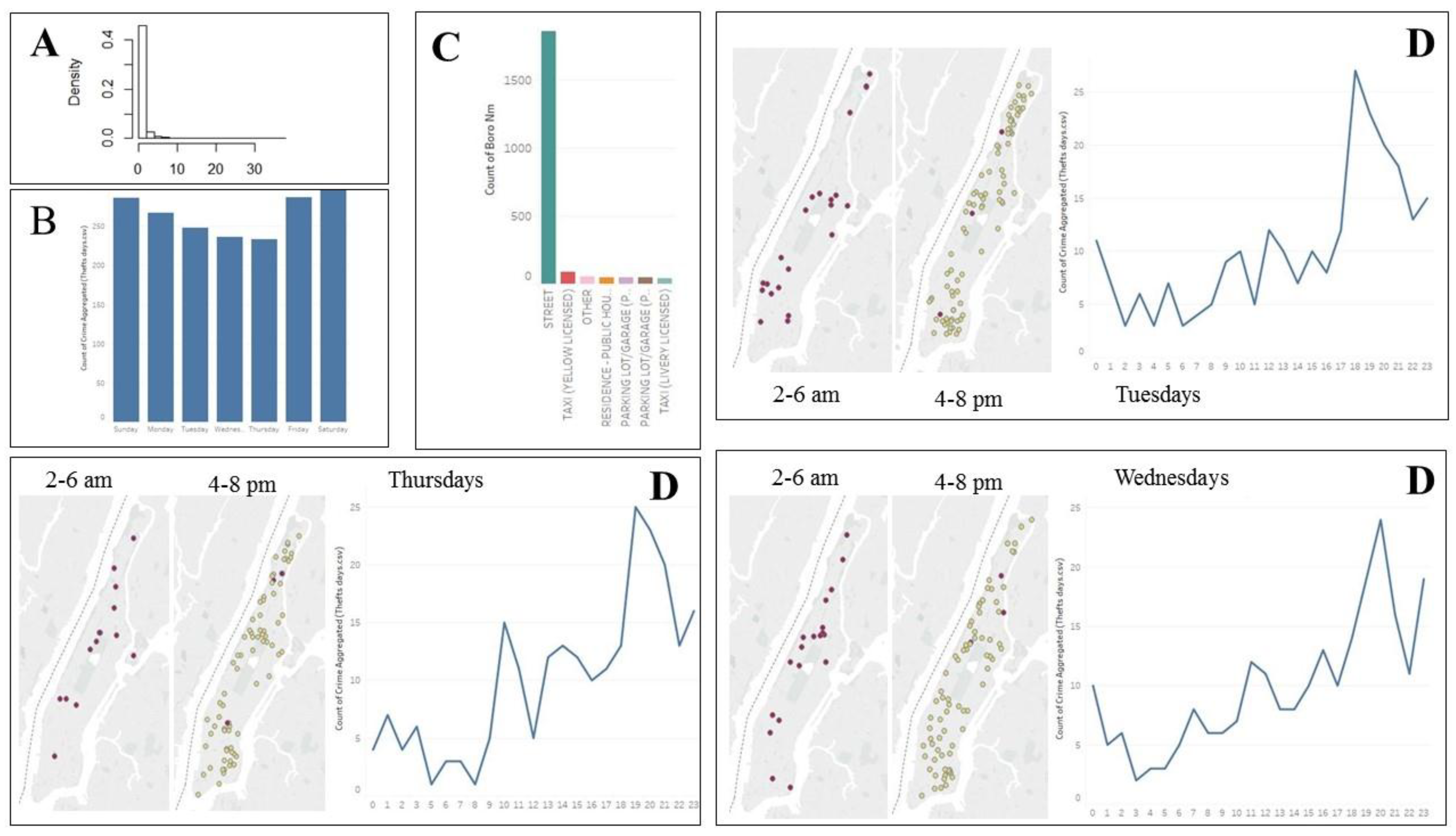
To build a good regression model, we checked data for missing values, multicollinearity, outliers, and normality. Missing values: After finding out the character of missing values, we excluded them from analysis. Multicollinearity: We wanted to avoid any two independent variables that are highly correlated (r > 0.9) because they create a multicollinearity problem in the regression model. Therefore, we performed a correlation analysis using the Pearson correlation coefficient, which describes the relation between variables in terms of linearity. However, after checking the variables, we did not find any independent variables that are strongly correlated. Therefore, we have no multicollinearity problem in our data. Additionally, checking the training set data for outliers did not result in any outliers. However, a normality check showed that data of four variables (thefts, restaurants, subway entrances, and graffiti) is strongly right-skewed (Figure 1A) because many street segments have zero values of thefts, restaurants, subway entrances, and graffiti. Therefore, we performed a logarithmic transformation of data within these four variables, previously adding one to all values to avoid log 0 cases. Logarithmic transformation of data significantly improved data distribution, and therefore, the transformed data in the training set was used to perform a correlation analysis to decide what variables to include in the regression analysis. Finally, we checked six assumptions for correctness of the prediction model and tested the prediction model on the test set data.
3. Results
3.1. Temporl and Spatial Distribution of Data
Exploration of day of week and theft variables does not demonstrate any significant trend (Figure 1B). However, the initial theft data analysis with Tableau revealed that almost all thefts from motor vehicles happen on streets (Figure 1C). Therefore, to investigate further, we used only thefts that occurred on streets. Time series analysis of thefts for each day within a week and the geospatial analysis of theft unveils a common pattern in both time series and theft mapping results for Tuesdays, Wednesdays, and Thursdays data (Figure 1D) with theft rates increasing from 4 p.m. to 7—8 p.m., and the lowest theft rates being at 2—6 a.m. However, we did not observe any pattern for any of the remaining week days, i.e., neither time series plots nor theft maps for different time ranges demonstrate any common trends. To check if criminal behaviors or opportunities for committing a theft depend on human activities during particular hours, we divided a week into time ranges based on human activities (weekday work hours, weekday commute hours, weekday nights, weekend nights, etc.). For each time range, we generated a map with theft rate for every street segment (Figure 2A). Visual comparative analysis of maps reveals that thefts from motor vehicles “move” within Manhattan depending on time range, and the intensity of theft is different depending on human activities.
To narrow our search from the most opportune days and time for committing a theft to territories where a theft is most likely to occur, we performed a hot spot analysis (Figure 2B). Hot spot analysis demonstrates the most potentially dangerous territories located in East Village and some spots in Uptown Manhattan, i.e., Washington Heights and Inwood, whereas the safest areas are Upper East Side and Financial District. The reason for the latter, however, appears to be restrictions on parking a private vehicle on many streets. In order to pinpoint the crime locations more accurately, we performed a correlation and regression analysis to find urban generators of thefts and, based on these generators, to come closer to the specific street segments with high theft prediction.
3.2. Selection of the Prediction Model
We trained eight different machine learning algorithms for the regression task on the training dataset with 12,794 samples and 10-fold cross validation with three repeats, tuning the following parameters: (1) For the linear regression, the intercept is included; (2) for the elastic-net, we use the tuned best-fit parameters lambda λ = 0 that corresponds to zero amount of shrinkage and the mixing parameter alpha α = 1 that performs the lasso fit; (3) for the SVM with a radial kernel, we use the tuned best-fit parameters cost C = 1 and gamma γ = 2.908401; (4) for the SVM with a linear kernel, we use the tuned best-fit parameter cost C = 1; (5) for the decision tree (CART), we tune the complexity parameter cp = 0.01185767; (6) for the bagged CART, we do not tune any hyperparameter; (7) for the random forest, we tune the number of trees to be 500 and mtry = 2; (8) for the stochastic gradient boosting (gbm), we tune the number of trees equal to 150, the maximum depth of variable interactions interaction.depth = 3, the shrinkage = 0.1, and the minimum number of observations in trees terminal nodes n.minobsinnode = 10. The number of thefts from motor vehicles committed in a street segment is the target variable (dependent variable). The number of subways, restaurants, graffiti, street pavement rating, and street segment width and length are the features (independent variables) used for the model selection by applying different machine learning methods. We computed RMSE and R2 for all built models and compared them in order to select the best prediction model. From the comparison results presented in the Table 2, it is obvious that linear models perform better on our data (linear regression, elastic-net), as well as the random forest. For the best regression model, we want to have the low error (close to zero) and the high variability of a target variable explained by the features (close to one). Although the lowest value of RMSEmin and the highest value of R2max are observed while using the random forest regression, we proceed with the mean values of RMSE and R2 obtained from the 10-fold cross validation with three repeats procedure. Therefore, we consider linear regression and elastic-net as candidate models having the lowest RMSEmean and the highest R2mean. Because the elastic-net increases bias to reduce overfitting (and, accordingly, to achieve lower variance) and none of our models suffer from overfitting, we choose linear regression as the final prediction model for thefts from motor vehicles. With linear regression, the model produces less bias, and preserves the same RMSE and R2.
3.3. Prediction Model Using Multiple Linear Regression
The Pearson correlation coefficient demonstrates a moderate positive linear relation between thefts and subway entrances (s_rho = 0.49, p-value < 2.2 × 10⁻¹⁶, a weak positive linear relation between thefts and restaurants, as well as thefts and graffiti (for both relations s_rho = 0.19, p-value < 2.2 × 10⁻¹⁶), a very weak positive linear relation between thefts and street pavement rating (s_rho = 0.02, p-value = 0.02153), and a very weak negative positive relation between thefts and street segment length (s_rho = −0.02, p-value = 0.01068), as well as thefts and street width (s_rho = −0.02, p-value = 0.005803). Variables having very weak relations with thefts are excluded from the regression (street pavement rating, street segment length, and street segment width).
During the building of the linear regression model, we considered the significant variables (subway entrances, restaurants, and graffiti). Then, if necessary, we dropped the one with the highest p-value until all p = values were reasonable (p-value < 0.05). The output of the multiple linear regression is presented in the Table 3.
In the Table 3 *** corresponds to the significance level 0.000.
With p-values < 0.05 for all variables, we conclude there is strong evidence against the null hypothesis, H0 that the predictors have no effect on the mean level of the response variable (thefts from motor vehicles). To examine if the prediction model is correct, we checked the following assumptions:
Assumption 1, “Mean of residuals is zero:” In our case, the assumption is met with mean of residuals equal to −2.278831 × 10⁻¹⁶.
Assumption 2, “Homoscedasticity of residuals or equal variance” (by checking residuals vs. fitted values): In our case, the assumption is met because the data is not evenly dispersed and does not form clusters on the residual vs. fitted graph.
Assumption 3, “No autocorrelation of residuals:” The assumption is met since the residuals are not autocorrelated. The computed Durbin-Watson statistic = 2.0326, p-value < 0.9717, and therefore, we accept the null hypothesis H0: Autocorrelation is not greater than 0.
Assumption 4, “The X variables and residuals are uncorrelatedL” The assumption is met, as all three variables are uncorrelated with residuals. For subways and residuals cor = 2.440349 × 10⁻¹⁶ with p-value = 1, for graffiti and residuals cor = 1.01497 × 10⁻¹⁵ with p-value = 1, for restaurants and residuals cor = −2.225019 × 10⁻¹⁶ with p-value = 1.
Assumption 5, “No multicollinearity:” Assumption is met for subways, restaurants, and graffiti VIF = 1. If VIF of a variable is high, the information in that variable is explained by other X variables present in the given model and the variable is redundant. Therefore, the lower VIF (<2) the better.
Assumption 6, “Normality of residuals:” Assumption is not met, as residuals are not normally distributed.
Since five of six assumptions are met, the prediction model is built correctly. However, the accuracy of the model is 77% (R-squared = 0.77), which implies that not all variables generating thefts from motor vehicles are considered in this research. Nonetheless, the test of this model on the test set demonstrates a good fit regarding error mean (Actual thefts—Predicted theft = 0.04692426) and correlation between actual and predicted thefts (cor = 0.8999567), even though residuals are not normally distributed.
3.4. Application of Research Results to Safer Parking
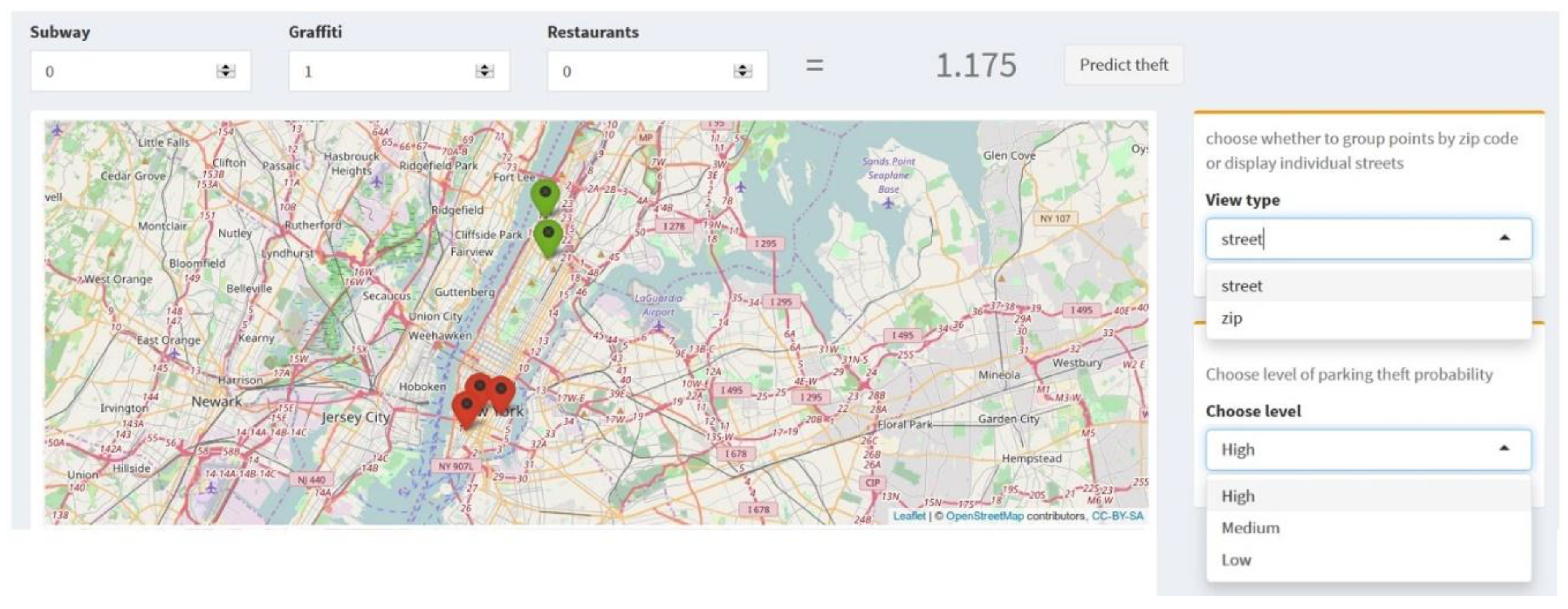
Using Shiny package for R, we developed the prototype of the application of our research results for safer parking that can be used by city dwellers, police, and insurance companies (Figure 3). City dwellers can find safety information for the selected street segment for the available parking. The developed Android App would take users’ provided street address or a current location into account and provide information about the parking safety in that location. It will also guide users to safe parking streets nearby. Police officers can use the application to allocate forces in risky areas. Insurance companies can tailor insurance prices for different cases based on users’ parking behavior. For instance, if a client lives and parks his motor vehicle on weekday nights and weekend days in Upper East Side, his motor vehicle is safe. If he works at daytime during weekdays and parks his vehicle close to his office in Midtown, he is safe too, as no significant hot spots of thefts are identified here. However, if he drives on weekend nights to East Village and parks his car there, this is where the trouble begins, as this area is identified as a hot spot of thefts from motor vehicles (with 99–95% confidence). Thus, an insurance company can offer a client the price regarding his parking behavior and locations during the week.
The application is based on the prediction model, where the predicted theft rate increases with the increase of number of subway entrances, graffiti, and restaurants. Therefore, all the variables with their values are mapped. Each street segment is associated with number of subway entrances, graffiti, and restaurants currently located on that segment. When a user chooses a street segment of his interest, he sees information about dependent variables there (number of subway entrances, graffiti, and restaurants), and the predicted value of thefts from motor vehicles is computed (based on data and prediction model) and displayed.
4. Discussion
The comparison of similar studies with our research results demonstrates that the biggest part of research is performed toward predicting hot sport or areas or neighborhoods, while predicting the exact location of crime to happen still remains the target for many researchers, data scientists, and crime analysts. Moreover, the majority of crime prediction models are built using data classification methods [42,43,44,45], differing from our research using regression methods. For instance, Bogomolov et al. [42] applied decision tree classifier based on the Breiman’s random forest and achieved accuracy of 70% while predicting if a specific urban area will be a crime hotspot or not using mobile phone and demographic data of London, UK. Antolos et al. [43] achieved accuracy of 74–83% while using the logistic regression to predict burglary based on the day of the week, time of the day, repeated victimization, connectors and barriers, id est., and historical crime data from 2010. Other machine learning approaches demonstrate reasonable accuracy when applying support vector machines (SVM) to predict crime hot spots [44], as well as Bayesian approach to predict the neighborhood where the next crime will happen [45]. The prediction model of homicides, a regression approach developed by Alves et al. [46] while using the random forest regression, achieves 97% accuracy.
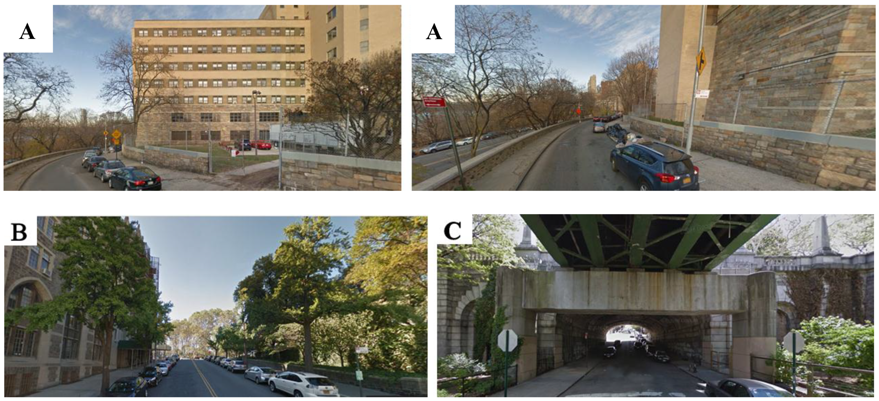
The most unsafe street segments are revealed by applying the search algorithm in ArcGIS. It is clear from the photographs (Figure 4A–C) that the urban reasons of these places being unsafe lay in not meeting the main principles of CPTED (Crime Prevention Through Environmental Design): Lack of natural surveillance (almost no observation from windows, no entrance doors, i.e., no “eyes on the street”), the nearest windows are too far to observe the environment or do not exist at all (walls and fences with no windows, i.e., ‘blind walls’), no inter-visibility of constructions (for instance, the fence is not inter-visible on Figure 4A), spaces are not frequently used by pedestrians, spaces are dark, and there is no lighting (Figure 4C), etc. In all the above-mentioned cases, the urban environment should be redesigned to make parking safer. If redesign of urban spaces is not possible, signs preventing parking should be placed on unsafe street segments.
The limitations of this research include an unsatisfactory determination coefficient of the prediction model (only 77% of variance in thefts from motor vehicles is explained by the independent variables), as well as automation of loading the updated data into the pipeline for making predictions up-to-date. The first limitation could be improved by adding more datasets and features in order to find other important variables that contribute to the theft rate increase or decrease. The second limitation requires to constantly obtain the newest data about the city and crime, to update the database, to load the new data into the pipeline, that includes data preprocessing, model building, testing, validation, and deployment, and to produce the predicted theft rates together with important factors. Moreover, continuing this research we would like to try other units for data aggregation—such as a square area within the city (for instance, 3 × 3 m, 10 × 10, or similar), instead of the street segment that we were using for this current research. As per the most recent research in machine learning/deep learning and urban science [42,47,48,49,50,51], we assume that using a square area of small granularity will bring our prediction closer to the exact location where and when a crime can happen.
Despite using several machine learning methods, we were not able to identify other significant urban factors using geospatial data analysis and machine learning tools because the open datasets on urban factors are limited or nonexistent. Therefore, in the future, we might implement more complex machine learning tools, such as object recognition, deep learning, etc., to detect urban factors in street views, and record, process, and extract knowledge from streetscape photo or video data. However, the methods we developed thus far should be useful in a general context for insurance companies and crime prevention in urban areas and have applications in risk management strategies for insurers.
5. Conclusions
The geospatial data of thefts from motor vehicles reveal some interesting patterns that suggest that human activity, as well as features of the urban environment, contribute to the frequency of crime. Time series analysis reveals a common theft pattern for Tuesdays, Wednesdays, and Thursdays with theft rates increasing from 4 p.m. to between 7 p.m. and 8 p.m., and the lowest theft rates being between 2 a.m. and 6 a.m. A plausible explanation for these observations is that while thefts might occur throughout the day, most are discovered and reported when people return to their vehicles after leaving their places of work. Similarly, when commuters leave the city during evenings and weekends, the number of cars exposed to theft decreases and crime reporting drops. Clearly, other explanations might also be possible.
The geospatial analysis of theft data demonstrates a spatial pattern of locations where thefts were committed on Tuesdays, Wednesdays, and Thursdays as well. It suggests that during the middle of the week, criminals’ behavior regarding thefts from motor vehicles has the same pattern, with similar opportunities for committing theft dictated by the urban environment, location of vulnerable motor vehicles, and other factors, such as the presence of witnesses and cameras. Moreover, visual comparative analysis of theft rates mapped on street segments demonstrates “movement” of thefts within Manhattan varying over time, such as the shifting intensity of theft, which diminishes during morning and evening commute hours. It demonstrates the dynamic nature of crime.
Hot spot analysis reveals the most crime-ridden areas are located in the East Village and some areas in Uptown Manhattan: Washington Heights and Inwood. The East Village has become more gentrified in recent years after previously being a bohemian neighborhood. Nowadays, it is known for a large variety of nightlife and is home to artists and diverse communities. Washington Heights used to be a territory for drug dealers with high crime rates, and Inwood is still one of the most unsafe neighborhoods in Manhattan, having many aging multifamily five- to eight-story buildings and almost no new construction. Comparing these results with theft rates for street segments within different time ranges might explain the hot spots of thefts: Once residents leave their apartments for work (around 7 a.m. to 8 a.m.), thefts begin to happen. The safest areas for car theft appear to be the Upper East Side and Financial District. In the Financial District, this may simply be a result of parking restrictions on private vehicles on many streets. However, there also appears to be a socioeconomic divide where thefts occur: Thefts are lower on the Upper East Side, where incomes are higher. This may reflect a greater concentration of crime prevention resources in these areas, such as the presence of police, private security, cameras, and doormen on duty. One practical result of these observations is that crime prevention resources can be concentrated in the appropriate areas at specific times and thereby increase the efficiency of resource utilization.
Applying eight different machine learning methods on the training set data with 10-fold cross validation with three repeats reveals that linear models perform better on our data (linear regression, elastic-net), as well as the random forest does. Though, due to random forest’s good performance on RMSEmin and R2max (but not on mean values of RMSE and R2), and because the elastic-net produces bias to reduce overfitting (though, overfitting does not occur in our case), we chose a linear regression to build the final prediction model. Multiple linear regression was useful in unveiling the following urban generators of thefts from motor vehicles: A higher number of subway entrances, graffiti, and restaurants on streets contributes to higher theft rates. Subway entrances, for example, might provide easy access and escape from an area after a crime is committed, as well as a greater flow of people who are not resident in the neighborhood. Although the prediction model for thefts meets almost all assumptions (five of six), its accuracy is not very high (only 77%), suggesting that there are other undiscovered factors making a contribution to the generation of thefts.
Author Contributions
Conceptualization, I.M.; methodology, I.M.; software, I.M., A.M., V.J.; validation, I.M.; formal analysis, I.M., A.M.; data curation, I.M.; writing—original draft preparation, I.M.; writing—review and editing, I.M.; visualization, I.M., A.M.; supervision, I.M.
Funding
This research received no external funding.
Acknowledgments
This work was conducted in collaboration with Liberty Mutual, Boston, MA. A special thank you for professor Sylvain Jaume for his advice and support.
Conflicts of Interest
The authors declare no conflict of interest.
References
- King, L.O. Comprehensive Sustainability Indicators: The Houston Sustainability Indicators Program. In Community Quality-of-Life Indicators: Best Cases VII; Holden, M., Philips, R., Stevens, C., Eds.; Springer International Publishing: London, UK, 2017; pp. 167–184. [Google Scholar]
- Armitage, R. Crime Prevention through Housing Design; Palgrave Macmillan: Hampshire, UK, 2013. [Google Scholar]
- Atlas, R.I. 21st Century Security and CPTED. Designing for Critical Infrastructure Protection and Crime Prevention, 2nd ed.; CRC Press, Taylor and Francis Group: Fort Lauderdale, FL, USA; Boca Raton, FL, USA, 2013. [Google Scholar]
- Cozens, P. Crime as an Unintended Consequence: Planning for Healthy Cities and the Need to Move beyond Crime Prevention through Environmental Design (CPTED). In Contemporary Issues in Australian Urban and Regional Planning; Brunner, J., Glasson, J., Eds.; Routledge: Abington, UK, 2015; pp. 230–250. [Google Scholar]
- Phillis, Y.A.; Koiukoglou, V.S.; Verdugo, C. Urban sustainability assessment and ranking of cities. Comput. Environ. Urban Syst. 2017, 64, 254–265. [Google Scholar] [CrossRef]
- Stafford, M.; Chandola, T.; Marmot, M. Association Between Fear of Crime and Mental Health and Physical Functioning. Am. J. Public Health 2007, 97, 2076–2081. [Google Scholar] [CrossRef] [PubMed] [Green Version]
- Stankevice, I.; Sinkiene, J.; Zaleckis, K.; Matijosaitiene, I.; Navickaite, K. What does a city master plan tell us about our safety? Comparative analysis of Vilnius, Kaunas and Klaipeda. Soc. Sci. 2013, 2–80, 64–76. [Google Scholar]
- Newman, O. Defensible Space: Crime Prevention through Urban Design; DIANE Publishing: New York, NY, USA, 1972. [Google Scholar]
- Jacobs, J. The Death and Life of Great American Cities; Random House: New York, NY, USA, 1961. [Google Scholar]
- Hillier, B.; Sahbaz, O. Crime and urban design: An evidence-based approach. In Designing Sustainable Cities; Cooper, R., Evans, G., Boycko, C., Eds.; Wiley-Blackwell: Singapore, 2009; pp. 163–186. [Google Scholar]
- Monteiro, L.T. The Valley of Fear—The morphology of crime, a case study in João Pessoa, Paraíba, Brasil. In Proceedings of the Eighth International Space Syntax Symposium; Greene, M., Reyes, J., Castro, A., Eds.; PUC: Santiago de Chile, Chile, 2012; pp. 3:01–3:17. [Google Scholar]
- Sypion-Dutkowska, N.; Leitner, M. Land use influencing the spatial distribution of urban crime. A case study of Szczecin, Poland. Int. J. Geo-Inf. 2017, 6–3, 74–97. [Google Scholar] [CrossRef]
- Cozens, P.; Saville, G.; Hillier, D. CPTED: A review and modern bibliography. Prop. Manag. 2005, 23–25, 328–356. [Google Scholar]
- Crowe, T.D. Crime Prevention through Environmental Design; Butterworth-Heinemann: Waltham, MA, USA, 2013. [Google Scholar]
- Jeffrey, C.R. Crime Prevention through Environmental Design; SAGE Publications: Beverly Hills, CA, USA, 1971. [Google Scholar]
- Kelling, G.L.; Wilson, J.Q. Broken windows. Atl. Mon. 1982, 249, 29–38. [Google Scholar]
- Saville, G.; Cleveland, G. Second-generation CPTED. The rise and fall of opportunity theory. In 21st Century Security and CPTED; Atlas, R.I., Ed.; CRC Press: Atlanta, GA, USA, 2008; pp. 91–105. [Google Scholar]
- Sutton, A.; Cherney, A.; White, R. Crime Prevention: Principles, Perspectives and Practices; Cambridge University Press: Cambridge, UK, 2014. [Google Scholar]
- Zahm, D. Using crime prevention through environmental design in problem-solving, Problem-oriented guides for police. Probl. Solving Tools Ser. Guide 2007, 8. Available online: http://www.popcenter.org/tools/pdfs/cpted.pdf (accessed on 7 February 2017).
- van Soomeren, P.; de Kleuver, J.; van de Klundert, V.; Junyent, A. High-rise in trouble. COST TU1203 Action. 2014. Available online: https://www.dsp-groep.nl/wp-content/uploads/18pv_High-rise_in_trouble-DSP-report.pdf (accessed on 7 February 2017).
- Ekblom, P.; Armitage, R.; Monchuk, L.; Castell, B. Crime Prevention Through Environmental Design in the United Arab Emirates: A Suitable Case for Reorientation? Built Environ. 2013, 39, 92–113. [Google Scholar] [CrossRef] [Green Version]
- Thorpe, A.; Gamman, L. Walking with Park: Exploring the ‘reframing’ and integration of CPTED principles in neighbourhood regeneration in Seoul, South Korea. Crime Prev. Community Saf. 2013, 15, 207–222. Available online: http://www.palgrave-journals.com/cpcs/journal/v15/n3/pdf/cpcs20136a.pdf (accessed on 7 February 2017). [CrossRef]
- Cozens, P.; Melenhorst, P. Exploring community perceptions of crime and crime prevention through environmental design (CPTED) in Botswana. In Proceedings of the British Criminology Conference; Millie, A., Ed.; Edge Hill University: Lancashire, UK, 2014; pp. 65–83. [Google Scholar]
- Lourenco, M.; Mann, P.; Paes, A.; Oliveira, D. SiAPP: An Information System for Crime Analytics Based on Logical Relational Learning. In Proceedings of the XII Brazilian Symposium on Information Systems on Brazilian Symposium on Information Systems: Information Systems in the Cloud Computing Era-Volume 1, Florianopolis, Brazil, 17–20 May 2016; pp. 1–23. [Google Scholar]
- Boldt, M.; Borg, A. Evaluating Temporal Analysis Methods Using Residential Burglary Data. Int. J. Geo-Inf. 2016, 5–9, 148–170. [Google Scholar] [CrossRef]
- Mburu, L.W.; Bakillah, M. Modeling spatial interactions between areas to assess the burglary risk. Int. J. Geo-Inf. 2016, 5, 47–63. [Google Scholar] [CrossRef]
- Du, Y.; Law, J. How do vegetation density and transportation network density affect crime across an urban central-peripheral gradient? A case study in Kitchener—Waterloo, Ontario. Int. J. Geo-Inf. 2016, 5, 118–141. [Google Scholar] [CrossRef]
- Marco, M.; Gracia, E.; López-Quílez, A. Linking neighborhood characteristics and drug-related police interventions: A Bayesian spatial analysis. Int. J. Geo-Inf. 2017, 6, 65–78. [Google Scholar] [CrossRef]
- NYC Open Data. 2017. Available online: https://opendata.cityofnewyork.us/ (accessed on 3 November 2018).
- Mitchell, A. The ESRI Guide to GIS Analysis; ESRI Press: Redlands, CA, USA, 2005; Volume 2. [Google Scholar]
- Getis, A.; Ord, J.K. The Analysis of Spatial Association by Use of Distance Statistics. Geogr. Anal. 1992, 24, 189–206. [Google Scholar] [CrossRef]
- Ord, J.K.; Getis, A. Local Spatial Autocorrelation Statistics: Distributional Issues and an Application. Geogr. Anal. 1995, 27, 286–306. [Google Scholar] [CrossRef]
- Scott, L.; Warmerdam, N. Extend Crime Analysis with ArcGIS Spatial Statistics Tools in ArcUser Online; Esri: Redlands, CA, USA, 2005. [Google Scholar]
- The Official Site of the City of New York. 2017. Available online: http://www1.nyc.gov/ (accessed on 3 November 2018).
- New York City Department of Transportation. 2017. Available online: http://www.nyc.gov/html/dot/html/home/home.shtml (accessed on 3 November 2018).
- ESRI. 2018. Available online: http://www.esri.com/ (accessed on 3 November 2018).
- Hillier, B.; Iida, S. Network and psychological effects in urban movement. In Proceedings of the Spatial Information Theory Conference, Ellicottville, NY, USA, 14–18 September 2005; Cohn, A.G., Mark, D.M., Eds.; York Publishing Services: New York, NY, USA, 2005; pp. 475–490. [Google Scholar]
- Matijosaitiene, I. Combination of CPTED and space syntax for the analysis of crime. Safer Communities 2016, 15, 49–62. [Google Scholar] [CrossRef]
- Zou, H.; Hastie, T. Regularization and Variable Selection via the Elastic Net. J. R. Stat. Soc. Ser. B (Stat. Methodol.) 2005, 67, 301–320. [Google Scholar] [CrossRef]
- Grover, P. Gradient Boosting from Scratch. 2017. Available online: https://medium.com/mlreview/gradient-boosting-from-scratch-1e317ae4587d (accessed on 20 July 2018).
- Brownlee, J. A Gentle Introduction to the Gradient Boosting Algorithm for Machine Learning. 2016. Available online: https://machinelearningmastery.com/gentle-introduction-gradient-boosting-algorithm-machine-learning/ (accessed on 20 July 2018).
- Bogomolov, A.; Lepri, B.; Staiano, J.; Oliver, N.; Pianesi, F.; Pentland, A. Once upon a crime: Towards crime prediction from demographics and mobile data. In Proceedings of the 16th International Conference on Multimodal Interaction, Istanbul, Turkey, 12–16 November 2014; pp. 427–434. [Google Scholar]
- Antolos, D.; Liu, D.; Ludu, A.; Vincenzi, D. Burglary Crime Analysis Using Logistic Regression. In Human Interface and the Management of Information. Information and Interaction for Learning Culture Collaboration and Business; Lecture Notes in Computer Science; Springer: Berlin/Heidelberg, Germany, 2013; Volume 8018, pp. 549–558. [Google Scholar]
- Kianmehr, K.; Alhajj, R. Crime Hot-spots prediction using support vector machine. In Proceedings of the IEEE International Conference on Computer Systems and Applications, Dubai, UAE, 8 March 2006; pp. 952–959. [Google Scholar]
- Liao, R.; Wang, X.; Li, L.; Qinh, Z. A Novel Serial Crime Prediction Model Based on Bayesian Learning Theory. In Proceedings of the International Conference on Machine Learning and Cybernatics, Qingdao, China, 11–14 July 2013; pp. 1757–1762. [Google Scholar]
- Alves, L.G.A.; Ribeiro, H.V.; Rodrigues, F.A. Crime prediction through urban metrics and statistical learning. Phys. A Stat. Mech. Its Appl. 2018, 505, 435–443. [Google Scholar] [CrossRef] [Green Version]
- Ma, X.; Li, Y.; Cui, Z.; Wang, Y. Forecasting Transportation Network Speed Using Deep Capsule Networks with Nested LSTM Models. 2018. Available online: https://export.arxiv.org/ftp/arxiv/papers/1811/1811.04745.pdf (accessed on 28 March 2019).
- Zhao, L.; Song, Y.; Deng, M.; Li, H. Temporal Graph Convolutional Network for Urban Traffic Flow Prediction Method. 2018. Available online: https://arxiv.org/pdf/1703.01006.pdf (accessed on 28 March 2019).
- Wang, Y.; Zhang, D.; Liu, Y.; Dai, B.; Lee, L.H. Enhancing transportation systems via deep learning: A survey. Transp. Res. Part C Emerg. Technol. 2018, 99, 144–163. [Google Scholar] [CrossRef]
- Sabour, S.; Frosst, N.; Hinton, G.E. Dynamic routing between capsules. Adv. Neural Inf. Process. Syst. 2017, 3856–3866. Available online: https://arxiv.org/pdf/1710.09829.pdf (accessed on 28 March 2019).
- Lv, Y.; Duan, Y.; Kang, W.; Li, Z.; Wang, F.Y. Traffic flow prediction with big data: A deep learning approach. IEEE Trans. Intell. Transp. Syst. 2015, 16, 865–873. [Google Scholar] [CrossRef]
Figure 1.
(A). Histogram of restaurants. The data is strongly right-skewed, with the most of values equal to zeros. (B). When do thefts happen? The graph shows a slight, although not very significant, increase in theft rates on Fridays, Saturdays, and Sundays. (C). Where do thefts happen? Almost all thefts from motor vehicles in Manhattan happen on the street. (D). Where and when thefts happen: Identifying patterns. The temporal distribution (in terms of crime per hour) and the spatial distribution of thefts from motor vehicles reveal a common pattern in theft location and time on Tuesdays, Wednesday, and Thursdays. However, we do not observe any pattern for other weekdays.

Figure 2.
(A). Theft rates for street segments within different time ranges. The maps show that thefts from motor vehicles “move” within Manhattan depending on time, while the intensity of theft is different depending on human activities. (B). Hot spot analysis of thefts from motor vehicles. Significant theft hot spots (with 90–95–99% confidence level) are found in the East Village, Washington Heights, and Inwood neighborhoods, whereas significant cold spots (with 90–95–99% confidence level) are located in the Upper East Side and Financial District of Manhattan, NY.

Figure 3.
Application of the research results for safer parking. When a user chooses a street segment of his interest, he sees information about dependent variables there (number of subway entrances, graffiti, and restaurants as Subway, Restaurant, and Graffiti accordingly on the picture above), and the predicted value of thefts from motor vehicles is computed (based on the data and the prediction model) and displayed—as Predict theft on the picture above. Also, a user can choose how to display the location—using a street address or a zip code, and the level of theft rate to display—a high (red color), medium (yellow), or low (green).

Figure 4.
(A). Street segments with the highest theft rate in Manhattan: Department of Vascular Surgery. Urban reasons of unsafety: Lack of natural surveillance (no “eyes on the street”), nearest windows are far, fence is not inter-visible, and blind wall (wall with no windows or doors). (B) Street segments with the highest theft rate in Manhattan: Morningside Church & Sakura park. Urban reasons of unsafety: Pedestrians rarely use this space, no natural surveillance (almost no observation from windows, no entrance doors) with a church on one side and park on another. (C). Street segment with the third highest theft rate in Manhattan: West 138th Street. Urban reasons of unsafety: No natural surveillance, no lighting, no pedestrian flows, no closed-circuit television (CCTV) cameras, etc. Nothing meets CPTED (Crime Prevention Through Environmental Design) requirements for safety and security. Moreover, there is a sign in this tunnel permitting parking, and therefore, contributing to the availability of motor vehicles as targets for theft.


Table 1.
Final geospatial dataset (extract).
| ID | Latitude, Longitude | Segment Length | Segment Width | Thefts | Restaurants | Subway Entrances | Graffiti | Pavement Rating |
|---|---|---|---|---|---|---|---|---|
| 33 | −74.25287637435896 40.50762599010005, −74.25299942180904 40.50688186992653 | 229 | 33.58 | 1 | 2 | 0 | 0 | 6 |
| 35 | −74.25308030444408 40.51209961294924, −74.25299384780556 40.51206137595131 | 66 | 30 | 0 | 0 | 0 | 0 | 0 |
Table 2.
Comparison of prediction models using root mean square error (RMSE) and coefficient of determination (R2).
Table 2.
Comparison of prediction models using root mean square error (RMSE) and coefficient of determination (R2).
| Model | RMSEmin | RMSEmean | R2mean | R2max |
|---|---|---|---|---|
| Linear regression | 0.4407129 | 0.6049274 | 0.6303150 | 0.8730436 |
| Elastic-net | 0.4407129 | 0.6049274 | 0.6303150 | 0.8730436 |
| SVMRadial | 0.4548175 | 0.6387557 | 0.5693278 | 0.7638390 |
| SVMLinear | 0.4486161 | 0.6281775 | 0.6133442 | 0.8739586 |
| Decision tree (CART) | 0.4470269 | 0.6164779 | 0.6024365 | 0.8418731 |
| BaggedCART | 0.4393015 | 0.6114266 | 0.6154108 | 0.8664760 |
| Random forest | 0.4404932 | 0.6053636 | 0.6258950 | 0.9007527 |
| Stochastic Gradient Boosting | 0.4446763 | 0.6102181 | 0.6194829 | 0.8680953 |
Table 3.
Multiple linear regression for prediction of thefts from motor vehicles.
| Estimate | Std. Error | t Value | Pr (>|t|) | |
|---|---|---|---|---|
| Intercept | 0.051844 | 0.002463 | 21.05 | <2 × 10⁻¹⁶*** |
| Subway | 1.158844 | 0.018242 | 63.52 | <2 × 10⁻¹⁶*** |
| Graffiti | 0.125207 | 0.007937 | 15.77 | <2 × 10⁻¹⁶*** |
| Restaurant | 0.054781 | 0.004021 | 13.62 | <2 × 10⁻¹⁶*** |
© 2019 by the authors. Licensee MDPI, Basel, Switzerland. This article is an open access article distributed under the terms and conditions of the Creative Commons Attribution (CC BY) license (http://creativecommons.org/licenses/by/4.0/).
Share and Cite
MDPI and ACS Style
Matijosaitiene, I.; McDowald, A.; Juneja, V. Predicting Safe Parking Spaces: A Machine Learning Approach to Geospatial Urban and Crime Data. Sustainability 2019, 11, 2848. https://doi.org/10.3390/su11102848
AMA Style
Matijosaitiene I, McDowald A, Juneja V. Predicting Safe Parking Spaces: A Machine Learning Approach to Geospatial Urban and Crime Data. Sustainability. 2019; 11(10):2848. https://doi.org/10.3390/su11102848
Chicago/Turabian StyleMatijosaitiene, Irina, Anthony McDowald, and Vishal Juneja. 2019. "Predicting Safe Parking Spaces: A Machine Learning Approach to Geospatial Urban and Crime Data" Sustainability 11, no. 10: 2848. https://doi.org/10.3390/su11102848
Note that from the first issue of 2016, this journal uses article numbers instead of page numbers. See further details here.