Monthly Load Forecasting Based on Economic Data by Decomposition Integration Theory


1
Economics and Management School, North China Electric Power University, Changping District, Beijing 102206, China
2
Beijing Key Laboratory of New Energy and Low-Carbon Development (North China Electric Power University), Changping District, Beijing 102206, China
3
Institute of Smart Energy, North China Electric Power University, Changping District, Beijing 102206, China
*
Author to whom correspondence should be addressed.
Sustainability 2018, 10(9), 3282; https://doi.org/10.3390/su10093282
Submission received: 3 September 2018
/
Revised: 8 September 2018
/
Accepted: 10 September 2018
/
Published: 14 September 2018
(This article belongs to the Section Energy Sustainability)
Abstract
:Accurate load forecasting can help alleviate the impact of renewable-energy access to the network, facilitate the power plants to arrange unit maintenance and encourage the power broker companies to develop a reasonable quotation plan. However, the traditional prediction methods are insufficient for the analysis of load sequence fluctuations. The economic variables are not introduced into the input variable selection and the redundant information interferes with the final prediction results. In this paper, a set of the ensemble empirical mode is used to decompose the electricity consumption sequence. Appropriate economic variables are as selected as model input for each decomposition sequence to model separately according to its characteristics. Then the models are constructed by selecting the optimal parameters in the random forest. Finally, the result of the component prediction is reconstituted. Compared with random forest, support vector machine and seasonal naïve method, the example results show that the prediction accuracy of the model is better than that of the contrast models. The validity and feasibility of the method in the monthly load forecasting is verified.
1. Introduction
Power load forecasting plays a key role in the power system operation and electricity market activities. The forecasting is still more important because it is the base of schedule of power system operation [1,2]. Electricity comes from traditional coal-fired power generation, wind power generation [3,4], solar power generation [5,6], biomass power generation [7] and tidal power generation [8]. These directions also require accurate load forecasting. Many activities within the power system such as the maintenance scheduling of generators, renewable-energy integration and even the investment of power plants and power grids depend on the monthly load forecasting. In the electricity market the regulators monitor the activities based upon the forecasting load and power generators [9]. Customers and power brokers decide their action strategies.
Power load forecasting has been studied for decades [10]. Various models, novel algorithms, advanced techniques and ingenious tricks have been developed to improve forecasting accuracy [11,12]. It was based on SVR and fuzzy-rough with PSO algorithms to forecast the residential sector’s electricity demand. And the method can identify relevant variables for developing the forecasting model [13]. It discussed the effects of various models in energy planning and forecasting, with emphasis on the application of ANN in the field of load forecasting [14,15]. It introduced different power load forecasting models and combined regression model with machine learning model to forecast the power load of commercial buildings [16].
The time-series models present good performance with historical data. Taking exogenous variables into account, the econometric models have better forecasting capability [16]. The model combined dynamic model and fuzzy time series. When considering the weather factors, the prediction accuracy of the model was better than that of the traditional model [17]. It based on a hybrid model of autoregressive integrated moving average (ARIMA) and support vector machines (SVMs). The ARIMA was used to predict the linear fundamental part of the load and the SVM predicted the nonlinearly sensitive part of the load [18]. It considered many long memories seasonal data sets and combined Fuzzy Time Series and SARFIMA for short-term load forecasting [19].
Artificial Neural Networks, Support Vector Machine and other intelligence algorithms dominate in the forecasting field for their powerful approximation between the dependent variable and independent variables [20]. It used wavelet analysis to decompose historical load data and then used support vector machine and neural network to select appropriate parameters [21,22]. The single branch predictions for each sequence are separately made and each branch prediction results are reconstructed to achieve ultimate load forecasting [23]. It proposed the goa-svm model, which predicts short-term load for local climate conditions. The results show that the prediction accuracy was better than that of the traditional model and other mixed models [24]. A deep belief network model was incorporated into a feed-forward neural network. And the model was applied to short-term electricity load forecasting [25]. An improved empirical mode decomposition (EMD) model combined with Elman neural network was proposed to predict the building electricity load. Effectiveness of the proposed model was carried out to real-world engineering test case in comparison with other prediction models [26]. Neural network was combined with optimization techniques for finding optimal network parameters to reduce the forecasting error. Further, the proposed algorithm was integrated with neural network for the proper tuning of network parameters to solve the real-world problem of short term load forecasting [27]. It proposed an improved grey model to enhance the disadvantage of the general GM (1,1) model when the load mutation was large. A practical application verifies that, compared with the existing grey forecasting models. The proposed model is a stable and feasible forecasting model with a higher forecasting accuracy [28].
However, these functions require massive training samples and the performances are sensitive to model parameters and input. Until now, more efforts have been put to tune the model parameters and to select proper input. Wavelet Decomposition [29,30,31], Empirical Mode Decomposition(EMD) [32,33], Complete Ensemble Empirical Mode Decompositions with adaptive noise(CEEMDAN) [34] broke down the original sequence into several more regular sequences for modeling. The effectiveness of such techniques has been validated.
Random Forest (RF) is a novel machine learning algorithm developed in recent years [35,36,37,38]. RF is robust to the input and number of samples. The great advantage of RF has been validated in many forecasting contests. Someone proposed a short-term load predictor, able to forecast the next 24 h of load using RF [39].
The above traditional methods consider less economic data but in actual life, economic factors have a great impact on the load. The reason for the small consideration is that there are fewer economic data samples, more variables. There is redundancy between variables and the correlation between variables and load is low. So, the traditional method cannot solve this problem and random forest can solve the problem. At the same time, the law of medium and long-term load fluctuation is complicated and there may be multiple regular superpositions using EEMD decomposition. This paper uses random forests to overcome these problems for accurate monthly load forecasting.
The other sections of this paper are organized as follows: the basic principles and modeling process of EEMD and RF algorithms were introduced in the second section, then an experimental study of monthly electricity consumption forecasting was carried to validate the proposed method and the discussion and conclusion were made at the end section.
2. Methods
In the field of signal analysis, EMD is widely used in various engineering fields. Because it has obvious advantages in dealing with non-stationary and nonlinear data compared with other algorithms. Meanwhile, it has a high signal-to-noise ratio to guarantee data availability. In contrast to EMD, EEMD incorporates normally distributed white noise to aid analysis, which makes the signal continuous at different scales, thereby reducing the degree of modal aliasing. The introduction of the noise in load forecasting is mainly to resist the damage of bad data on the accuracy of prediction results and improve the robustness of the model.
The subsequent RF algorithm is an algorithm based on a combined decision tree. Because of its insensitivity to default on problems and its high tolerance to noise or outliers, it is widely used on the field of classification and regression. This paper uses RF algorithm to make use of its many advantages in the good adaptability of multiple data sets, excellent fitting ability and insensitivity to irrelevant variables.
2.1. EEMD Fundamental Principle
In the signal-processing process of EMD, if there is an uneven distribution of signal extreme points, modal aliasing problems will occur. In response to this problem, Huang proposed adding uniformly distributed white noise to the decomposed signal. The noise with a mean value of zero will be canceled out as the result after several times of average elimination on signals of different time scales. Specific steps are as follows:
- (1)
- Add a random uniform Gaussian white noise sequence to the original sequence to get the new sequence ;
- (2)
- Decompose the noise-added sequence into and a residual series using EMD;
- (3)
- Repeat steps (1) and (2) until a smooth decomposition signal is obtained;
- (4)
- Calculate the average value of each decomposed component as the result. N is the number of Gaussian white noise added
The result of EEMD is shown as Formula (4). After increasing the uniform distribution of white noise, the occurrence of modal aliasing can be well improved and the degree of coincidence of each Y_IMF component to the overall trend and the fluctuation trend can be improved.
2.2. RF Fundamental Principle
RF is a collection method that aggregates many decision tree predictions and there is no correlation between each decision tree. The representation of RF is mainly reflected in the random sampling of features when the specimen is put back into a random number of the samples (bootstraps) and a decision tree is constructed. The introduction of this randomness is very helpful to the performance improvement of RF. Because of it, RF is not easy to fall into over-fitting and has good noise immunity (e.g., Insensitive to default). The specific modeling steps are as follows:
- (1)
- Assume that the number of original data samples is N and the number of decision trees in RF is k. k decision trees are extracted from the N by resampling and the number of training specimens in each decision tree is n.
- (2)
- Assume that the feature dimension of the input variable is M and any feature set whose number is m (m < M and m remains unchanged) in M. Through these m features, the optimal splitting node is determined.
- (3)
- RF consists of the k decision trees that grow as much as possible and do not require pruning.
- (4)
- In the regression algorithm, the result of each decision tree is weighted and averaged to obtain the result.
2.3. Diebold Mariano Test
Diebold and Marino proposed the DM test to determine whether a model’s predictive power is significantly different from another model [40]. Specific assumptions are as follows:
Formulas (5) and (6) are the null hypothesis and alternative hypothesis of the DM test, respectively and are the prediction errors between actual values and forecasted values of the different models and the function is the loss function of forecasting errors.
In Formula (7) is the sample mean loss differential difference and is the length of forecasting values.
From Formula (8) we can see the DM value converges to the normal distribution. is the zero-spectral density and is a consistent estimate of the asymptotic variance of . So, after calculating DM value , we draw a conclusion by comparing with from the standard normal distribution table. If is less than , we can accept the null hypothesis and consider the difference between the predictive powers of the two models to be inconspicuous. For example, if ≤ 1.96, we accept the null hypothesis. Otherwise, > 1.96, then the null hypothesis is rejected at the 5% level.
2.4. Modeling Process
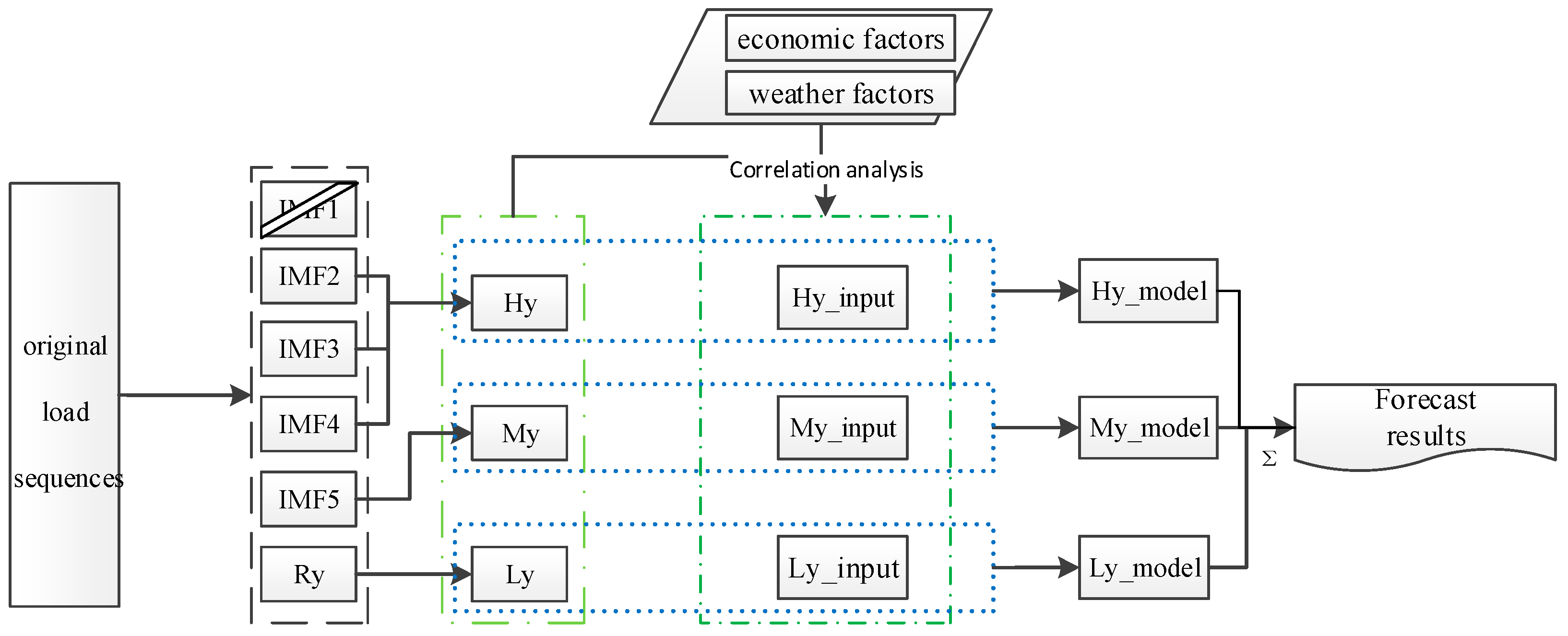
The specific modeling process is shown in Figure 1. The process is divided into three parts. First, the primary, secondary, tertiary industry and residential electricity original sequences are respectively decomposed into six components of Y_IMF1~Y_IMF5 and Y_R by EEMD. Then combine them into three components of high, medium and low frequency separately excepting Y_IMF1. Because the fluctuation frequency of Y_IMF1 is too large to be suitable for modeling. Secondly, the combined sequences are used for correlation analysis with economic and weather variables. The factors with higher correlation are selected as the input of different frequency models. Thirdly, the models are established by using the selected input and relative target value. Afterwards, the predicted values of different frequency sequences of different industries can be obtained through the models. The monthly load of the industry can be obtained by adding different frequency sequences of the same industry.
These industrial loads add up to the total social load.
3. Empirical Research
3.1. Data Description and Data Processing
This article adopts the China’s electricity consumption data from July 2009 to November 2017 from the National Bureau of Statistics of China and some power company. The electricity consumptions of primary, secondary, tertiary industries and resident are shown in Figure 2. Table A1 shows the input variables of economic and weather factors for modeling.
To avoid the influence of seasonal factors and other cyclical factors in the forecast results, the growth rate forecast method is adopted to handle four original power load sequences and the growth rate is to compare the data of the previous year.
In the prediction sequence, there is a lack of power consumption data for December 2009~2012. There are two main methods for missing data imputation. One is to use the 7~11 month-on-year growth average to reverse the missing data from 2013. The other is to use the average of the electricity consumption in December in the second half of the year to calculate the missing data. The specific method is selected based on the estimated errors in 2013~2017.
3.2. Data Set Division and Experimental Evaluation Index
Data sets are divided into training sets, validation sets and test sets according to different time spans. The goal of this article is to make accurate monthly load forecasts for the next six months, so the data from June to November of 2017 will be set as the final test set. The data of six months before November 2016 are randomly selected as the validation set for adjusting experimental parameters and verifying the effectiveness of the algorithm. The rests are training set for training models.
Based on the monthly national load demand forecast, this paper selects the mean absolute error (MAE), mean absolute percentage error (MAPE) and root mean square error (RMSE) as evaluation indicators. The expression is:
Among them, is a real value. is a prediction value and is the number of selected prediction points. If the obtained MAPE is tinier, there is smaller difference between predicted value and actual load value. It shows that the prediction is more accurate.
3.3. Analysis of Specific Modeling Process
3.3.1. EEMD Factorization Variable
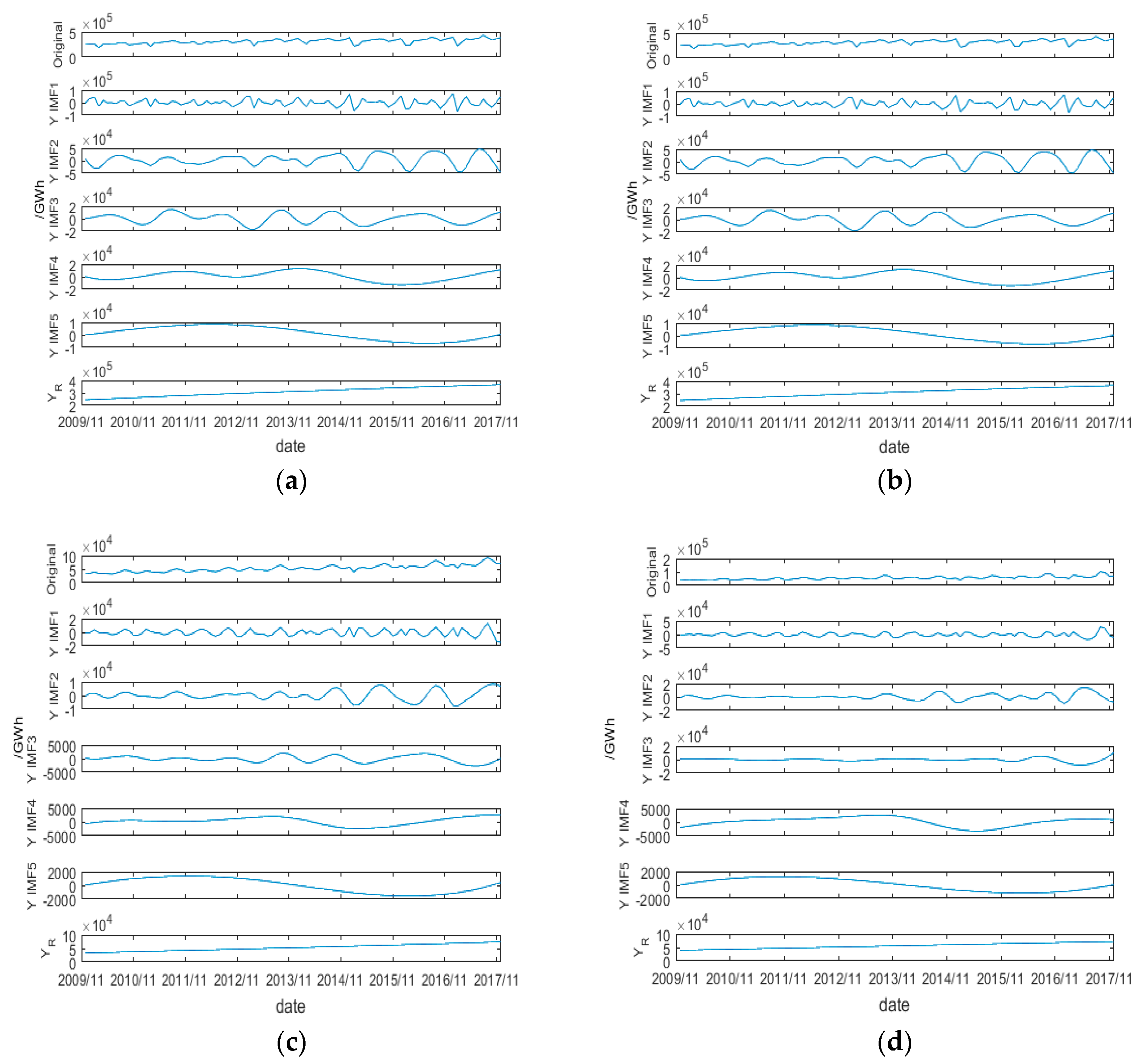
Use EEMD to decompose the primary, secondary, tertiary industrial electricity and residential electricity consumption sequences that need to be predicted. Since July 2009 to November 2017, there are 101 sets of data. In this paper, the electricity consumption is predicted two quarters ahead of time and the influential factors in the third quarter before the forecast periods are selected as the initial input variables. Because of the growth forecast, the data for the initial 12 months will be used as a basis. So, the N that needs to be decomposed is 80 (101 − 6 − 3 – 12 = 80). The number of components after EEMD can be obtained by the Formula (8), where the fix is rounded to 0. The number of solution scores is 5. The decomposition results are shown in Figure 3.
m = fix(log2(N)) − 1
In the process of EEMD decomposing the four original sequences into five components (Y_IMF1~Y_IMF5) and one residual component Y_R respectively, the standard deviation of added Gaussian white noise (Nstd) is 0.2 and the number of noise added is 100. From the decomposition of EEMD in Figure 3, it is unfavorable for the RF modeling prediction in the later period that the frequency of some component oscillations is very fast, so the high-frequency Y_IMF1 is discarded. For the latter low-frequency sequences, the components are superposed and combined in order to avoid that the single decomposition sequence has too great influence on the prediction accuracy. The combination method is that Y_IMF2, Y_IMF3 and Y_IMF4 make up high-frequency data. Y_IMF5 is regarded as a medium frequency sequence (My) and remainder Y_R is regarded as a low-frequency sequence (Ly).
3.3.2. Random Forest Modeling
Since the lead time of this paper is set at six months, the input of random forest is the external economic and weather index from seventh to the ninth before the predicted month. The total number of one month’s relevant indices that can be found is 303. If you enter all the three-month indices into the model, it will undoubtedly bring infinite challenges to the complexity and accuracy of the model. To simplify the model and improve the accuracy of the model, this paper introduces the Kendall correlation coefficient to filter the input variables of the corresponding different frequency sequences of varied industry. By controlling the size of the correlation and the Kendall coefficient return value p, the final size of each model input variable is controlled to be between 15 and 40. Although random forests are highly inclusive for redundant data, proper screening of variables can also improve model prediction accuracy. Meanwhile, random forest is the tree regression model that does not require normalization of selected input variables. However, when the comparison models are established, the input variables must be normalized to remove the dimension of the variables.
In the RF modeling of high, medium and low frequency sequences, the number of random forests is the key to the effect on the model. Using MAPE as a criterion, RF modeling was performed on 50 to 1500 trees in the training set. In the case of different numbers of trees, the verification set MAPE behaves as shown in Figure 4.
From Figure 4, we can see that in the random forest modeling process of the first industry, the different frequency models achieve the optimal at 250 (5 × 50), 50 (1 × 50) and 50 (1 × 50) trees respectively. In the verification, the MAPE of the model is the smallest showing excellent adaptability. The test set modeling is then modeled using its optimal number. Similarly, it can be concluded that the best number of high, medium and low frequency data for the secondary and tertiary industries and residential electricity consumption are respectively 50 (1 × 50), 550 (11 × 50), 100 (2 × 50), 550 (11 × 50), 400 (8 × 50), 50 (1 × 50), 900 (18 × 50), 400 (8 × 50), 350 (7 × 50).
3.3.3. Cross Validation and Contrast Model Establishment
The models are tested multiple times with the set validation set before final testing. The validation set is randomly selected from data other than the test set. Table A2 shows six verification set errors.
This paper selects SVM and seasonal naïve method that has been approved by many experts and scholars in recent years for comparative analysis and compares the effect of adding EEMD on the accuracy of the model. Input variable selection methods of RF and SVM are the same as before. Among them, the SVM needs to be normalized to the input before modeling. Seasonal naïve method only needs to be used for preliminary finishing of the original four power sequences.
4. Results Analysis
The model prediction results are divided into three parts. One is the forecast of electricity consumption by sub-industries. The second part is the forecast of the total social electricity consumption superimposed on the electricity consumption of sub-industries and the last part is the completion of the whole society electricity forecast for the simple use of combination forecasts. At the same time, because there is no essential difference between RMSE and MAE in a single month calculation, only MAE is marked in the table and RMSE is used as a reference when comparing results. The primary, secondary and tertiary industries and residential forecast results are shown in Table 1.
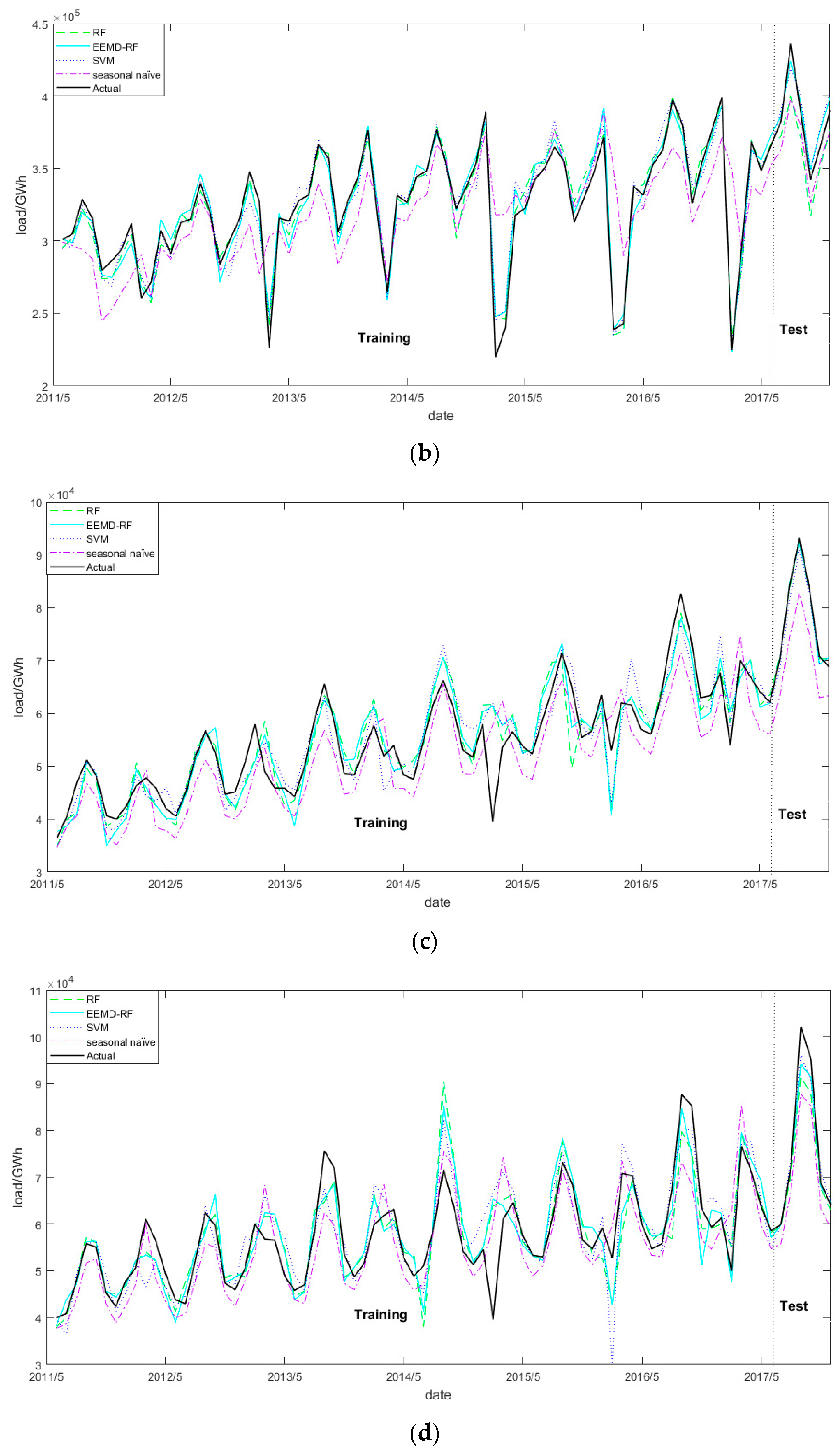
The sub-industry fit and prediction curve is shown in Figure 5. The left side of the vertical line is the fitted curve and the right side is the predicted curve. It can be seen from the fitting curve that seasonal naïve method has a poor fitting effect, because of reflecting volatility earlier or later.
After comparing the four methods of MAE, MAPE and RMSE, it was found that the EEMD-RF model about primary industry had the highest degree of agreement with MAE of 298.96 GWh, MAPE of 2.90% and RMSE of 340.35 GWh. The SVM and RF that were not processed by EEMD were the next with MAE of 451.16 and 509.14 GWh, MAPE of 3.47% and 4.01% and RMSEs of 580.89 and 606.84 GWh. The poor performance of seasonal naïve method in the primary industry forecast is since the algorithm does not reflect the external changes in time. When the EEMD is not used for decomposition the RF cannot recognize the increase in the error caused by the external weather-related load.
The secondary industry fit and prediction curve is shown in Figure 5b. After the three evaluation criteria, the same EEMD-RF model was found to have the highest degree of agreement with MAE of 8255.49 GWh, MAPE of 2.14% and RMSE of 8752.63 GWh. The performance of SVM and seasonal naïve method followed with MAE of 11,380.77 and 17,887.41 GWh, MAPE of 2.91% and 4.55% and RMSE of 12,127.78 and 20,437.14 GWh. The RF model has the same problems as the primary industry forecast. Under the premise of setting a long lead time, the useful information cannot be distinguished well and the accuracy of the model is reduced. In the secondary industry forecast, EEMD optimizes its input variables for RF where the impact of noise is less than the benefits of the EEMD decomposition variables, so the results increase slightly.
The tertiary industry fitting and prediction curve is shown in Figure 5c. After comparing, the RF model was found to be in leading state and the MAE was 607.10 GWh, the MAPE was 0.82% and the RMSE was 774.37 GWh. The RF treated with EEMD and SVM performed second with MAE of 908.27 and 1848.28 GWh, MAPE of 1.22% and 2.37% and RMSE of 1090.27 and 8405.35 GWh. The good fit into the RF model is related to the third industry load characteristics. The tertiary industry is mainly the service industry. The load of such industries is relatively stable and there is no obvious fluctuation in demand. In the parameter, selection is not taken into account but a large-scale input like other industries into the model. This makes the RF insensitivity to the variables fully utilized and achieves results higher than the EEMD decomposition model.
The residential electricity fitting and prediction curve is shown in Figure 5d. Residual electricity forecast results can be found from Table 1. The forecasting effect was consistent with that of the secondary industry. The EEMD-RF model had the highest degree of agreement with MAE of 2212.13 GWh, MAPE of 2.33% and RMSE of 3630.70 GWh. The SVM model and RF followed with MAE of 2607.08 and 3764.43 GWh, MAPE of 3.01% and 4.14% and RMSE of 3312.32 and 5401.80 GWh, respectively. The seasonal naïve method performed poorest.
For each method, the six-months electricity consumption forecast of the whole society is shown in Table 2. We can see that the best method is the EEMD-RF method with MAPE of 1.34% and MAE of 7447 GWh. Followed by SVM and RF, EEMD-RF accuracy stands out. The seasonal naïve method provides a comparison index, which proves that other algorithms have certain feasibility.
The two methods EEMD-RF and SVM with the best average effect on the verification set are used to perform combined forecasting. The two methods are simply averaged to obtain the final forecast result, as shown in Table 3. From the combined forecasting results, we can see that the last forecasting accuracy is about 10% higher than that of the single model, with the MAE raised to 6828 GWh and the MAPE raised to 1.24%. However, this completely depends on the average fitness of the selected model. If there is a poor fit of a single model, it can easily affect the effect of its combined forecast. This is why we have to give up the direct modeling of SVM and RF.
5. Discussion
DM test is used to verify the validity of the model being developed. All other models were compared to the EEMD-RF model. According to the DM test principle proposed above, the null hypothesis is that the prediction abilities of the two models are similar and the other hypothesis is that there are significant differences in the prediction performance of the two models. Table 4 shows us the DM value about EEMD-RF and other models with MAE and MAPE.
Except for residential electricity DM value less than 1.960, other values are more than 1.960. It indicates that the EEMD-RF model is different from the other models at a 5% significance level in sub-industry load forecasting. Thus, the null hypothesis could be rejected at a 5% significance level. The DM value of residential electricity is less than 1.960 and greater than 1.645, indicating EEMD-RF model is different from RF and SVM at a 10% significance level. Thereby, the null hypothesis could be rejected at a 10% significance level. Therefore, the proposed EEMD-RF model significantly outperforms the other models.
6. Conclusions
In this paper, the input of the model, the optimization of the model parameters and combinatorial prediction are used to forecast the electricity load of the whole population in China. On the model input, selecting the economic data from the National Bureau of Statistics of China as the model input increases the accuracy of the model by about 15% over the pure use of power data and other data. At the same time, EEMD is used to decompose the prediction sequence, analyze the original sequence fluctuation trend and improve the correlation between the predictor and the input variable. In the optimization of model parameters due to fewer random variables in the RF, similar enumeration method is used to complete model optimization in a certain range of values. The idea of aggregation is respectively embodied in the model after EEMD decomposition, the prediction results are added together and the accuracy of the model is improved through the combination of prediction methods.
By applying EEMD and RF to the national monthly electricity usage data, it was found that the improved model achieved better accuracy than the traditional SVM and the error was reduced by 10~25% compared to the single random forest. It reflects the dynamic characteristics of the original sequence and verifies the effectiveness of the method in monthly load forecasting. At the same time, the advantage of using RF for variable insensitivity is reduced and the prediction error caused by unstable noise to the model is reduced, the model generalization ability is improved and it can be applied to different prediction fields. Because there are steps in the EEMD of the later reconstruction pre-diction results when each component is modeled in a RF merely the effects of a unitary model is considered. The parameters that make the single model topgallant are sought and the global optimum results cannot be obtained, only getting the sub-optimal results. Therefore, we can continue to carry out the next stage research on how to achieve the optimal parameters of combined forecasting.
Author Contributions
Conceptualization, D.L.; Data curation, K.S.; Formal analysis, K.S.; Funding acquisition, D.L.; Software, K.S.; Writing—original draft, K.S.; Writing—review & editing, H.H. and P.T.
Funding
This research was funded by the National Natural Science Foundation of China (NSFC) (51641701), the 111 Project (B18021) and the Fundamental Research Funds for the Central Universities (2017MS080).
Conflicts of Interest
The authors declare no conflict of interest.
Appendix A

Table A1.
Number and meaning of input variables.
| Number | Meaning | Number | Meaning |
|---|---|---|---|
| 001 | average temperature | 153 | Export value of metal products export growth (%) |
| 002 | Average maximum temperature | 154 | Export value of general equipment manufacturing industry increased by year (%) |
| 003 | Mean minimum temperature | 155 | Export value of special equipment manufacturing industry increased by year (%) |
| 004 | Absolute maximum temperature | 156 | Export value of electrical machinery and equipment manufacturing industry increased by year (%) |
| 005 | Absolute minimum temperature | 157 | Export delivery value of computers, telecommunications and other electronic equipment manufacturing industry increased by year (%) |
| 006 | Precipitation | 158 | Export value of instrument manufacturing industry increased by year (%) |
| 007 | The number of days of precipitation equal to or greater than 1 mm | 159 | Exports of other manufacturing exports increased year-on-year (%) |
| 008 | The number of days of precipitation equal to or greater than 0.1 mm | 160 | Export delivery value of waste comprehensive utilization industry increased by year (%) |
| 009 | The number of snow days | 161 | The delivery value of electricity, heat production and supply industry increased by year (%) |
| 010 | Storm days | 162 | The delivery value of gas production and supply industry increased by year (%) |
| 011 | Foggy days | 163 | The delivery value of water production and supply industry increased by year (%) |
| 012 | Frost days | 164 | The value of cargo throughput at the port scale above sea level (ten thousand tons) |
| 013 | Maximum temperature (reliability index) | 165 | The current value of the throughput of foreign trade goods (ten thousand tons) |
| 014 | Minimum temperature (reliability index) | 166 | Value of freight volume (ten thousand tons) |
| 015 | Precipitation (reliability index) | 167 | The current value of railway freight volume (ten thousand tons) |
| 016 | Industrial producer purchasing price index (same month last year = 100) | 168 | The current value of highway freight volume (ten thousand tons) |
| 017 | Fuel and power purchase price index (same month last year = 100) | 169 | Current value of water transport freight volume (ten thousand tons) |
| 018 | Black metal material purchase price index (same month last year = 100) | 170 | Current value of civil aviation freight volume (ten thousand tons) |
| 019 | Purchase price index of nonferrous metals and wires (same month last year = 100) | 171 | Turnover of goods turnover (100 million tons) |
| 020 | Purchase price index of chemical raw materials (same month last year = 100) | 172 | The current value of railway freight turnover (hundreds of millions of tons) |
| 021 | Wood and pulp purchase price index (same month last year = 100) | 173 | The current value of highway cargo turnover (100 million tons) |
| 022 | Purchase price index of building materials and nonmetallic minerals (same month last year = 100) | 174 | The current value of the turnover of waterborne goods (hundreds of millions of tons) |
| 023 | Purchase price index of other industrial raw materials and semi-finished products (same month last year = 100) | 175 | Civil aviation cargo turnover current value (100 million tons) |
| 024 | Purchase price index of agricultural and sideline products (same month last year = 100) | 176 | Value of passenger traffic volume (ten thousand people) |
| 025 | Purchase price index of textile raw materials (same month last year = 100) | 177 | The value of railway passenger traffic volume (ten thousand people) |
| 026 | Producer price index for industrial producers (same month last year = 100) | 178 | Traffic volume of highway passenger volume (ten thousand people) |
| 027 | Producer price index of producer goods (same month last year = 100) | 179 | Water transport passenger traffic volume (10,000 people) |
| 028 | Producer price index of producer of living goods (same month last year = 100) | 180 | Passenger volume of civil aviation passenger volume (10,000 people) |
| 029 | Producer price index of producer goods (same month last year = 100) | 181 | Turnover of passenger turnover (100 million kilometers) |
| 030 | Producer price index of producer goods for mining industry (same month last year = 100) | 182 | Railway passenger turnover in the current period (100 million kilometers) |
| 031 | Producer price index of producer goods for raw material industry (same month last year = 100) | 183 | Highway passenger turnover in the current period (100 million kilometers) |
| 032 | Processing industry producer goods producer price index (same month last year = 100) | 184 | Water transport passenger turnover rate (100 million kilometers) |
| 033 | Producer price index of producer of living goods (same month last year = 100) | 185 | Civil aviation passenger turnover in the current period (100 million kilometers) |
| 034 | Producer price index for food industry producers (same month last year = 100) | 186 | Cumulative value of total retail sales of consumer goods ($100 million) |
| 035 | Clothing factory producer price index (same month last year = 100) | 187 | Retail value of clothing, shoes, hats, needles and textile commodities: cumulative value (100 million yuan) |
| 036 | Producer price index for general consumer goods manufacturers (same month last year = 100) | 188 | Cumulative value of retail sales of clothing commodities (100 million yuan) |
| 037 | Durable consumer goods producer price index (same month last year = 100) | 189 | Cumulative value of retail sales of cosmetics commodities (100 million yuan) |
| 038 | Producer price index for metallurgical industry (same month last year = 100) | 190 | Cumulative value of retail sales of household appliances and audio-visual equipment (100 million yuan) |
| 039 | Producer price index for power producers (same month last year = 100) | 191 | Cumulative value of retail sales of furniture commodities (100 million yuan) |
| 040 | Producer price index of coal and coking industry producers (same month last year = 100) | 192 | Cumulative value of retail sales of building and decoration materials (100 million yuan) |
| 041 | Producer price index for oil producers (same month last year = 100) | 193 | Value of gold, silver and jewelry retail sales value (100 million yuan) |
| 042 | Producer price index of chemical industry (same month last year = 100) | 194 | Cumulative value of retail sales of grain, oil, food, beverages, cigarettes and alcoholic drinks (100 million yuan) |
| 043 | Producer price index for machinery industry (same month last year = 100) | 195 | Cumulative value of grain, oil and food retail sales (100 million yuan) |
| 044 | Producer price index for producer of building materials industry (same month last year = 100) | 196 | Cumulative value of retail sales of beverage commodities ($100 million) |
| 045 | Producer price index of forest industry producer (same month last year = 100) | 197 | Cumulative value of retail value of tobacco and wine commodities (billion yuan) |
| 046 | Producer price index of food industry (same month last year = 100) | 198 | Cumulative value of retail sales of other commodities ($100 million) |
| 047 | Producer price index of textile industry (same month last year = 100) | 199 | Cumulative value of retail sales of automobile commodities (100 million yuan) |
| 048 | Producer price index for sewing industrial producers (same month last year = 100) | 200 | Cumulative value of retail value of daily use commodities (billion yuan) |
| 049 | Producer price index of leather industry producer (same month last year = 100) | 201 | Cumulative value of retail sales of petroleum and products (100 million yuan) |
| 050 | Producer price index for producer of paper industry (=100 of last year) | 202 | Cumulative value of retail sales of books, magazines and magazines (100 million yuan) |
| 051 | Producer price index of industrial and cultural arts and Crafts Industrial producer (same month last year = 100) | 203 | Cumulative value of retail sales of sports and entertainment commodities (100 million yuan) |
| 052 | Producer price index for other industrial producers (same month last year = 100) | 204 | Cumulative value of retail sales of communications equipment (100 million yuan) |
| 053 | Producer price index for industrial producers (same month last year = 100) | 205 | Cultural and office goods retail value (100 million yuan) |
| 054 | Industrial producer price index for coal mining and washing industry (same month last year = 100) | 206 | Cumulative value of retail sales of Chinese and Western medicines (100 million yuan) |
| 055 | Producer price index for industrial producer of oil and natural gas (=100 of last year) | 207 | Cumulative value of real estate construction area (10,000 square meters) |
| 056 | Black metal ore mining industry producer price index (same month last year = 100) | 208 | Cumulative area of newly built real estate (10,000 square meters) |
| 057 | Producer price index of industrial producer of nonferrous metal mining industry (same month last year = 100) | 209 | Cumulative value of completed area of real estate (10,000 square meters) |
| 058 | Producer price index of industrial producer of non-metallic mineral industry (=100 of last year) | 210 | Accumulative value of construction area of office building (ten thousand square meters) |
| 059 | Ex-factory price index for mining and auxiliary activities (=100 of last year) | 211 | The total area of newly built office buildings is accumulated (10,000 square meters) |
| 060 | Producer price index of industrial producers in agricultural and sideline products processing industry (same month last year = 100) | 212 | Accumulated value of office building area (10,000 square meters) |
| 061 | Producer price index of industrial producers in food industry (=100 of last year) | 213 | Accumulative value of construction area of commodity residence (ten thousand square meters) |
| 062 | Ex-factory price index for industrial producers of wine, beverages and refined tea (same month last year = 100) | 214 | Cumulative area of newly built commercial housing area (ten thousand square meters) |
| 063 | Producer price index for industrial products in tobacco industry (same month last year = 100) | 215 | Accumulated value of the completed area of a commodity house (ten thousand square meters) |
| 064 | Producer price index of textile industrial producers (same month last year = 100) | 216 | Cumulative area of commercial business space (10,000 square meters) |
| 065 | Producer price index of industrial producer of textile, clothing and apparel industry (same month last year = 100) | 217 | The accumulative value of construction area for commercial business premises (10,000 square meters) |
| 066 | Ex-factory price index for leather, fur, feather and its products and footwear manufacturers (same month last year = 100) | 218 | Cumulative area of commercial business space (10,000 square meters) |
| 067 | Ex-factory price index for timber processing and industrial producer of wood, bamboo, rattan, brown and straw products (same month last year = 100) | 219 | Cumulative value of sales area of office buildings (10,000 square meters) |
| 068 | Furniture producer industrial producer price index (same month last year = 100) | 220 | The total sales area of office buildings (10,000 square meters) |
| 069 | Producer price index for industrial producers of paper and paper products (same month last year = 100) | 221 | The total sales area of office buildings will be accumulated (10,000 square meters) |
| 070 | Printing and recording media reproduction industry producer price index (same month last year = 100) | 222 | Cumulative value of commodity housing sales area (10,000 square meters) |
| 071 | Producer price index for industrial producers in culture, education, industry, sports and entertainment products (same month last year = 100) | 223 | The total sales area of commercial housing is accumulated (10,000 square meters) |
| 072 | Petroleum, coal and other fuel processing industry producer price index (same month last year = 100) | 224 | The total sales area of commercial housing will be accumulated (10,000 square meters) |
| 073 | Producer price index for industrial producers of chemical raw materials and chemical products (same month last year = 100) | 225 | Accumulative value of sale area of commodity house (ten thousand square meters) |
| 074 | Factory producer price index for pharmaceutical manufacturers (same month last year = 100) | 226 | The total sales area of commercial housing is about 10,000 square meters |
| 075 | Producer price index for industrial producer of chemical fiber industry (same month last year = 100) | 227 | The total sales area of commercial housing will be accumulated (10,000 square meters) |
| 076 | Producer price index for industrial producer of rubber and plastic products (same month last year = 100) | 228 | The total sales area of commercial business space is accumulated (10,000 square meters) |
| 077 | Ex-factory price index for industrial producers of non-metallic mineral products (same month last year = 100) | 229 | The total sales area of commercial business premises is accumulated (10,000 square meters) |
| 078 | Producer price index of industrial producers in ferrous metal smelting and calendaring processing industry (same month last year = 100) | 230 | The total sales area of commercial business premises will be accumulated (10,000 square meters) |
| 079 | Producer price index of industrial producers in nonferrous metal smelting and calendaring processing industry (same month last year = 100) | 231 | Total value of office building sales ($100 million) |
| 080 | Ex-factory price index for industrial producers of metal products (same month last year = 100) | 232 | Total value of present house sales of office building (100 million yuan) |
| 081 | Producer price index for industrial producer of general equipment manufacturing (=100 of last year) | 233 | Total value of office building sales volume ($100 million) |
| 082 | Producer price index of industrial producer for special equipment manufacturing industry (same month last year = 100) | 234 | Cumulative value of commodity housing sales ($100 million) |
| 083 | Ex-factory price index for industrial vehicle manufacturers (same month last year = 100) | 235 | Accumulative value of present house sales of commodity housing (billion yuan) |
| 084 | Ex-factory price index for industrial producers in railways, ships, aerospace and other transport equipment manufacturing industries (same month last year = 100) | 236 | Cumulative value of commodity housing sales volume ($100 million) |
| 085 | Producer price index of industrial producer for electrical machinery and equipment manufacturing (=100 of last year) | 237 | Cumulative value of commodity house sales ($100 million) |
| 086 | Producer price index for industrial producer computers, telecommunications and other electronic equipment manufacturers (same month last year = 100) | 238 | Accumulative value of present housing sales of commodity house (billion yuan) |
| 087 | Industrial producer price index for instrument manufacturing industry (same month last year = 100) | 239 | Cumulative value of commodity house sales volume ($100 million) |
| 088 | Producer price index for other manufacturing industries (same month last year = 100) | 240 | Cumulative value of commercial business housing sales ($100 million) |
| 089 | Ex-factory price index of industrial producer of waste comprehensive utilization industry (=100 of last year) | 241 | The total value of existing commercial housing sales is 100 billion yuan |
| 090 | Metal producer, machinery and equipment repair industry producer price index (same month last year = 100) | 242 | Cumulative sales value of commercial business premises (100 million yuan) |
| 091 | Producer price index of industrial producers in electricity, heat production and supply industries (same month last year = 100) | 243 | Cumulative value of land acquisition area of real estate (10,000 square meters) |
| 092 | Producer price index of industrial producer for gas production and supply industry (same month last year = 100) | 244 | Accumulated value of land transaction price of real estate industry (billion yuan) |
| 093 | Producer price index of industrial producers in water production and supply industry (same month last year = 100) | 245 | Cumulative value of real estate investment ($100 million) |
| 094 | Cumulative value of export value of industrial exports (100 million yuan) | 246 | Cumulative value of real estate investment ($100 million) |
| 095 | Cumulative value of export value of coal mining and washing industry (100 million yuan) | 247 | Cumulative value of housing investment of 90 square meters and below (100 million yuan) |
| 096 | Cumulative value of export value of oil and natural gas extraction industry (100 million yuan) | 248 | Cumulative value of housing investment over 144 square meters (billion yuan) |
| 097 | The cumulative value of export value of non-ferrous metal mining and export industry (100 million yuan) | 249 | Accumulative value of villa and high-grade apartment investment (billion yuan) |
| 098 | Cumulative value of export value of non-metallic ore mining and export industry (100 million yuan) | 250 | Total value of investment in real estate office building (100 million yuan) |
| 099 | Export value of agricultural and sideline products processing industry accumulated value (100 million yuan) | 251 | Cumulative value of investment in commercial real estate business (100 million yuan) |
| 100 | The cumulative value of the export delivery value of the food manufacturing industry (100 million yuan) | 252 | Cumulative value of other real estate investment ($100 million) |
| 101 | Export value of liquor, beverages and refined tea manufacturing industry value accumulated (100 million yuan) | 253 | Cumulative value of investment in real estate development and construction projects (100 million yuan) |
| 102 | The cumulative value of the export delivery value of the tobacco products industry (billion yuan) | 254 | Cumulative value of investment in real estate development and installation projects (100 million yuan) |
| 103 | The cumulative value of the export delivery value of the textile industry (100 million yuan) | 255 | Cumulative value of investment in real estate equipment and equipment purchase (100 million yuan) |
| 104 | Export value of textile, clothing and apparel industry accumulated value (100 million yuan) | 256 | Cumulative value of other investment in real estate investment ($100 million) |
| 105 | Export value of leather, fur, feathers and their products and footwear industry accumulated value (100 million yuan) | 257 | Real estate land purchase fee accumulative value (100 million yuan) |
| 106 | Export value of timber processing, timber, bamboo, rattan, brown and straw products accumulated value (100 million yuan) | 258 | Total investment of real estate development plan (100 million yuan) |
| 107 | Total value of export delivery value of furniture manufacturing industry (billion yuan) | 259 | Added value of fixed assets investment in real estate development (100 million yuan) |
| 108 | Export value of paper and paper products, accumulated value (100 million yuan) | 260 | Accumulative value of the source of investment funds of real estate (billion yuan) |
| 109 | Cumulative value of export delivery value of printing and recording media reproduction industry (100 million yuan) | 261 | Accumulated value of capital surplus in real estate investment last year (100 million yuan) |
| 110 | The total value of delivery value of exports of culture, education, industry, sports and entertainment products (100 million yuan) | 262 | Real estate investment this year, the total amount of funds is accumulated (100 million yuan) |
| 111 | Export value of oil, coal and other fuel processing industry accumulated value (100 million yuan) | 263 | Real estate investment domestic loan accumulative value (billion yuan) |
| 112 | Export value of chemical raw materials and chemical products manufacturing value accumulated value (100 million yuan) | 264 | Total value of investment and utilization of foreign investment in real estate investment (billion yuan) |
| 113 | The cumulative value of the export delivery value of the pharmaceutical manufacturing industry (100 million yuan) | 265 | Accumulative value of self-financing of real estate investment (billion yuan) |
| 114 | Cumulative value of export value of chemical fiber manufacturing industry (100 million yuan) | 266 | Cumulative value of other funds for real estate investment ($100 million) |
| 115 | Export value of non-metallic mineral products industry accumulated value (100 million yuan) | 267 | The total value of the real estate investment should be paid ($100 million) |
| 116 | Export value of ferrous metal smelting and calendaring processing industry value accumulated value (100 million yuan) | 268 | Cumulative value of real estate investment projects ($100 million) |
| 117 | Export value of non-ferrous metal smelting and calendaring processing industry value accumulated value (100 million yuan) | 269 | Fixed long distance telephone call duration (IP) and current value (ten thousand minutes) |
| 118 | The cumulative value of the export delivery value of the metal products industry (100 million yuan) | 270 | The value of a long term (ten thousand minutes) for a mobile phone call |
| 119 | Export value of general equipment manufacturing industry accumulated value (100 million yuan) | 271 | End value of subscriber number (ten thousand households) at the end of a fixed phone |
| 120 | Export value of special equipment manufacturing industry: cumulative value (100 million yuan) | 272 | End of user number (10,000) at the end of city phone year |
| 121 | Export value of electrical machinery and equipment manufacturing industry accumulated value (100 million yuan) | 273 | End of user number (ten thousand households) at the end of rural telephone year |
| 122 | Export value of computers, telecommunications and other electronic equipment manufacturing industry accumulated value (100 million yuan) | 274 | Terminal value of mobile phone users (10,000 households) |
| 123 | Export value of instrument manufacturing industry: cumulative value (100 million yuan) | 275 | Mobile SMS business volume (100 million) |
| 124 | Cumulative value of export value of other manufacturing exports ($100 million) | 276 | Number of letters in the current period (100 million) |
| 125 | Cumulative value of export delivery value of waste resources comprehensive utilization industry (100 million yuan) | 277 | The value of the number of packages (10,000 pieces) |
| 126 | Cumulative value of delivery value of electricity, heat production and supply industry (100 million yuan) | 278 | The current value of the bill of exchange (ten thousand) |
| 127 | Cumulative value of delivery value of gas production and supply industry (100 million yuan) | 279 | Number of newspapers in the current period (ten thousand) |
| 128 | The cumulative value of delivery value of water production and supply industry (100 million yuan) | 280 | Number of magazines in the current period (ten thousand) |
| 129 | Year-on-year increase in export value of industrial exports (%) | 281 | Value of express volume (10,000 pieces) |
| 130 | Export value of coal mining and washing industry increased by year (%) | 282 | The current value of the total telecommunications business (100 million yuan) |
| 131 | Export value of oil and natural gas extraction industry grew by year on year (%) | 283 | The end value of the supply of money and quasi money (M2) |
| 132 | The delivery value of non-ferrous metal mining and export industry increased by year (%) | 284 | Monetary and quasi currency (M2) supply growth (%) |
| 133 | The delivery value of non-metallic ore mining and export industry increased by year (%) | 285 | Money (M1) supply terminal value (billion) |
| 134 | Export value of agricultural and sideline products processing industry increased by year (%) | 286 | Money (M1) supply growth (%) |
| 135 | Food manufacturing export delivery value increase (%) | 287 | Cash (M0) supply at the end of the period (billion yuan) |
| 136 | Export value of wine, beverages and refined tea manufacturing increased by year (%) | 288 | Cash (M0) supply in circulation increased year-on-year (%) |
| 137 | Export value of tobacco products export growth (%) | 289 | Consumer price index (=100 of the same month of the previous year) |
| 138 | Export delivery value of textile industry increase (%) | 290 | Consumer price index for food, tobacco and alcoholic drinks (same month last year = 100) |
| 139 | Export value of textile, clothing and apparel industry increased by year (%) | 291 | Clothing consumer price index (same month last year = 100) |
| 140 | Export value of leather, fur, feather and its products and footwear industry increased by year (%) | 292 | Consumer price index for residential residents (same month last year = 100) |
| 141 | Export value of timber processing and timber, bamboo, rattan, brown and straw products increased by year (%) | 293 | Consumer price index for consumer goods and services (same month last year = 100) |
| 142 | Export value of furniture manufacturing export increase (%) | 294 | Consumer price index for transport and communications (=100 of last year) |
| 143 | Export delivery value of paper and paper products increased year by year (%) | 295 | Education, culture and entertainment consumer price index (same month last year = 100) |
| 144 | Export delivery value of printing and recording media replication industry increased year by year (%) | 296 | Consumer price index for health care residents (same month last year = 100) |
| 145 | The delivery value of exports of culture, education, industry, sports and entertainment products increased by year (%) | 297 | Consumer price index for other supplies and services (=100 of last year) |
| 146 | Export value of oil, coal and other fuel processing industries increased by year (%) | 298 | Food consumer price index (same month last year = 100) |
| 147 | Export value of chemical raw materials and chemical products manufacturing increased by year (%) | 299 | Food consumer price index (same month last year = 100) |
| 148 | Increase in export delivery value of pharmaceutical manufacturing industry (%) | 300 | The consumer price index of egg residents (=100 of the same month of the same year) |
| 149 | Export value of chemical fiber manufacturing industry increased by year (%) | 301 | Consumer price index for aquatic products (same month last year = 100) |
| 150 | Export value of non-metallic mineral products industry increased by year (%) | 302 | Fresh vegetable consumer price index (same month last year = 100) |
| 151 | Export value of ferrous metal smelting and calendaring processing industry increased by (%) | 303 | Fresh fruit consumer price index (same month last year = 100) |
| 152 | Export value of non-ferrous metal smelting and calendaring processing industry increased by (%) |
Table A2.
Verification set error.
| V1 | V2 | V3 | V4 | V5 | V6 | ||
|---|---|---|---|---|---|---|---|
| primary | MAE | 0.034 | 0.017 | 0.075 | 0.061 | 0.068 | 0.050 |
| RMSE | 0.040 | 0.022 | 0.088 | 0.065 | 0.091 | 0.052 | |
| MAPE | 0.035 | 0.016 | 0.082 | 0.064 | 0.063 | 0.050 | |
| secondary | MAE | 0.037 | 0.046 | 0.043 | 0.035 | 0.013 | 0.028 |
| RMSE | 0.064 | 0.058 | 0.061 | 0.045 | 0.015 | 0.031 | |
| MAPE | 0.038 | 0.048 | 0.045 | 0.033 | 0.012 | 0.027 | |
| tertiary | MAE | 0.027 | 0.025 | 0.021 | 0.028 | 0.019 | 0.027 |
| RMSE | 0.030 | 0.028 | 0.024 | 0.040 | 0.022 | 0.029 | |
| MAPE | 0.025 | 0.024 | 0.019 | 0.027 | 0.018 | 0.025 | |
| residential | MAE | 0.046 | 0.026 | 0.044 | 0.034 | 0.045 | 0.036 |
| RMSE | 0.052 | 0.029 | 0.053 | 0.036 | 0.058 | 0.047 | |
| MAPE | 0.043 | 0.025 | 0.041 | 0.032 | 0.046 | 0.034 | |
| all | MAE | 0.100 | 0.068 | 0.079 | 0.092 | 0.036 | 0.049 |
| RMSE | 0.110 | 0.103 | 0.099 | 0.112 | 0.045 | 0.076 | |
| MAPE | 0.024 | 0.017 | 0.020 | 0.023 | 0.009 | 0.012 |
References
- Guo, H.; Chen, Q.; Xia, Q.; Kang, C.; Zhang, X. A monthly electricity consumption forecasting method based on vector error correction model and self-adaptive screening method. Int. J. Electr. Power Energy Syst. 2018, 95, 427–439. [Google Scholar] [CrossRef]
- Liu, D.; Ruan, L.; Liu, J.; Huan, H.; Zhang, G.; Feng, Y.; Li, Y. Electricity consumption and economic growth nexus in beijing: A causal analysis of quarterly sectoral data. Renew. Sustain. Energy Rev. 2018, 82, 2498–2503. [Google Scholar] [CrossRef]
- Liu, D.; Wang, J.; Wang, H. Short-term wind speed forecasting based on spectral clustering and optimised echo state networks. Renew. Energy 2015, 78, 599–608. [Google Scholar] [CrossRef]
- Foley, A.M.; Leahy, P.G.; Marvuglia, A.; McKeogh, E.J. Current methods and advances in forecasting of wind power generation. Renew. Energy 2012, 37, 1–8. [Google Scholar] [CrossRef] [Green Version]
- Diagne, M.; David, M.; Lauret, P.; Boland, J.; Schmutz, N. Review of solar irradiance forecasting methods and a proposition for small-scale insular grids. Renew. Sustain. Energy Rev. 2013, 27, 65–76. [Google Scholar] [CrossRef]
- Pieri, E.; Kyprianou, A.; Phinikarides, A.; Makrides, G.; Georghiou, G.E. Forecasting degradation rates of different photovoltaic systems using robust principal component analysis and arima. IET Renew. Power Gener. 2017, 11, 1245–1252. [Google Scholar] [CrossRef]
- Ferreira, L.R.A.; Otto, R.B.; Silva, F.P.; Souza, S.N.M.D.; Souza, S.S.D.; Junior, O.H.A. Review of the energy potential of the residual biomass for the distributed generation in brazil. Renew. Sustain. Energy Rev. 2018, 94, 440–455. [Google Scholar] [CrossRef]
- Theo, W.L.; Lim, J.S.; Ho, W.S.; Hashim, H.; Lee, C.T. Review of distributed generation (DG) system planning and optimisation techniques: Comparison of numerical and mathematical modelling methods. Renew. Sustain. Energy Rev. 2017, 67, 531–573. [Google Scholar] [CrossRef]
- O’Connell, N.; Pinson, P.; Madsen, H.; O’Malley, M. Benefits and challenges of electrical demand response: A critical review. Renew. Sustain. Energy Rev. 2014, 39, 686–699. [Google Scholar] [CrossRef]
- Pappas, S.S.; Ekonomou, L.; Moussas, V.C.; Karampelas, P.; Katsikas, S.K. Adaptive load forecasting of the hellenic electric grid. J. Zhejiang Univ.-Sci. A (Appl. Phys. Eng.) 2008, 9, 1724–1730. [Google Scholar] [CrossRef]
- Khan, A.R.; Mahmood, A.; Safdar, A.; Khan, Z.A.; Khan, N.A. Load forecasting, dynamic pricing and dsm in smart grid: A review. Renew. Sustain. Energy Rev. 2016, 54, 1311–1322. [Google Scholar] [CrossRef]
- Ahmad, A.S.; Hassan, M.Y.; Abdullah, M.P.; Rahman, H.A.; Hussin, F.; Abdullah, H.; Saidur, R. A review on applications of ann and svm for building electrical energy consumption forecasting. Renew. Sustain. Energy Rev. 2014, 33, 102–109. [Google Scholar] [CrossRef]
- Son, H.; Kim, C. Short-term forecasting of electricity demand for the residential sector using weather and social variables. Resour. Conserv. Recycl. 2017, 123, 200–207. [Google Scholar] [CrossRef]
- Debnath, K.B.; Mourshed, M. Forecasting methods in energy planning models. Renew. Sustain. Energy Rev. 2018, 88, 297–325. [Google Scholar] [CrossRef]
- Ekonomou, L.; Christodoulou, C.; Mladenov, V. A short-term load forecasting method using artificial neural networks and wavelet analysis. Int. J. Power Syst. 2016, 1, 64–68. [Google Scholar]
- Yildiz, B.; Bilbao, J.I.; Sproul, A.B. A review and analysis of regression and machine learning models on commercial building electricity load forecasting. Renew. Sustain. Energy Rev. 2017, 73, 1104–1122. [Google Scholar] [CrossRef]
- Lee, W.-J.; Hong, J. A hybrid dynamic and fuzzy time series model for mid-term power load forecasting. Int. J. Electr. Power Energy Syst. 2015, 64, 1057–1062. [Google Scholar] [CrossRef]
- Nie, H.; Liu, G.; Liu, X.; Wang, Y. Hybrid of arima and SVMs for short-term load forecasting. Energy Procedia 2012, 16, 1455–1460. [Google Scholar] [CrossRef]
- Sadaei, H.J.; Guimarães, F.G.; José da Silva, C.; Lee, M.H.; Eslami, T. Short-term load forecasting method based on fuzzy time series, seasonality and long memory process. Int. J. Approx. Reason. 2017, 83, 196–217. [Google Scholar] [CrossRef]
- Voyant, C.; Notton, G.; Kalogirou, S.; Nivet, M.-L.; Paoli, C.; Motte, F.; Fouilloy, A. Machine learning methods for solar radiation forecasting: A review. Renew. Energy 2017, 105, 569–582. [Google Scholar] [CrossRef]
- Deo, R.C.; Tiwari, M.K.; Adamowski, J.F.; Quilty, J.M. Forecasting effective drought index using a wavelet extreme learning machine (w-elm) model. Stoch. Environ. Res. Risk Assess. 2017, 31, 1211–1240. [Google Scholar] [CrossRef]
- Wang, S.; Zhang, N.; Wu, L.; Wang, Y. Wind speed forecasting based on the hybrid ensemble empirical mode decomposition and ga-bp neural network method. Renew. Energy 2016, 94, 629–636. [Google Scholar] [CrossRef]
- Xia, C.; Zhang, M.; Cao, J. A hybrid application of soft computing methods with wavelet svm and neural network to electric power load forecasting. J. Electr. Syst. Inf. Technol. 2017. [Google Scholar] [CrossRef]
- Barman, M.; Dev Choudhury, N.B.; Sutradhar, S. A regional hybrid goa-svm model based on similar day approach for short-term load forecasting in Assam, India. Energy 2018, 145, 710–720. [Google Scholar] [CrossRef]
- Dedinec, A.; Filiposka, S.; Dedinec, A.; Kocarev, L. Deep belief network based electricity load forecasting: An analysis of macedonian case. Energy 2016, 115, 1688–1700. [Google Scholar] [CrossRef]
- Liu, Y.; Wang, W.; Ghadimi, N. Electricity load forecasting by an improved forecast engine for building level consumers. Energy 2017, 139, 18–30. [Google Scholar] [CrossRef]
- Singh, P.; Dwivedi, P. Integration of new evolutionary approach with artificial neural network for solving short term load forecast problem. Appl. Energy 2018, 217, 537–549. [Google Scholar] [CrossRef]
- Jin, M.; Zhou, X.; Zhang, Z.M.; Tentzeris, M.M. Short-term power load forecasting using grey correlation contest modeling. Expert Syst. Appl. 2012, 39, 773–779. [Google Scholar] [CrossRef]
- Rana, M.; Koprinska, I. Forecasting electricity load with advanced wavelet neural networks. Neurocomputing 2016, 182, 118–132. [Google Scholar] [CrossRef]
- Bahrami, S.; Hooshmand, R.-A.; Parastegari, M. Short term electric load forecasting by wavelet transform and grey model improved by pso (particle swarm optimization) algorithm. Energy 2014, 72, 434–442. [Google Scholar] [CrossRef]
- Liu, J.P.; Li, C.L. The short-term power load forecasting based on sperm whale algorithm and wavelet least square support vector machine with dwt-ir for feature selection. Sustainability 2017, 9, 1188. [Google Scholar] [CrossRef]
- Qiu, X.; Ren, Y.; Suganthan, P.N.; Amaratunga, G.A.J. Empirical mode decomposition based ensemble deep learning for load demand time series forecasting. Appl. Soft Comput. 2017, 54, 246–255. [Google Scholar] [CrossRef]
- Fan, G.F.; Qing, S.; Wang, H.; Hong, W.C.; Li, H.J. Support vector regression model based on empirical mode decomposition and auto regression for electric load forecasting. Energies 2013, 6, 1887–1901. [Google Scholar] [CrossRef]
- Zhang, W.; Qu, Z.; Zhang, K.; Mao, W.; Ma, Y.; Fan, X. A combined model based on ceemdan and modified flower pollination algorithm for wind speed forecasting. Energy Convers. Manag. 2017, 136, 439–451. [Google Scholar] [CrossRef]
- Yajima, H.; Derot, J. Application of the random forest model for chlorophyll-a forecasts in fresh and brackish water bodies in Japan, using multivariate long-term databases. J. Hydroinform. 2018, 20, 206–220. [Google Scholar] [CrossRef]
- Lahouar, A.; Ben Hadj Slama, J. Hour-ahead wind power forecast based on random forests. Renew. Energy 2017, 109, 529–541. [Google Scholar] [CrossRef]
- Lei, C.; Deng, J.; Cao, K.; Ma, L.; Xiao, Y.; Ren, L. A random forest approach for predicting coal spontaneous combustion. Fuel 2018, 223, 63–73. [Google Scholar] [CrossRef]
- Wang, Z.; Wang, Y.; Zeng, R.; Srinivasan, R.S.; Ahrentzen, S. Random forest based hourly building energy prediction. Energy Build. 2018, 171, 11–25. [Google Scholar] [CrossRef]
- Lahouar, A.; Ben Hadj Slama, J. Day-ahead load forecast using random forest and expert input selection. Energy Convers. Manag. 2015, 103, 1040–1051. [Google Scholar] [CrossRef]
- Diebold, F.X.; Mariano, R.S. Comparing predictive ability. J. Bus. Econ. Stat. 1995, 13, 253–262. [Google Scholar]
Figure 1.
Monthly load forecasting flow chart based on EEMD-RF. (Notes: Hy: High frequency sequence; My: Medium frequency sequence; Ly: Low frequency sequence).
Figure 1.
Monthly load forecasting flow chart based on EEMD-RF. (Notes: Hy: High frequency sequence; My: Medium frequency sequence; Ly: Low frequency sequence).

Figure 2.
(a) the primary industry electricity consumption; (b) the secondary industry electricity consumption; (c) the tertiary industry electricity consumption; (d) the residential electricity consumption.
Figure 2.
(a) the primary industry electricity consumption; (b) the secondary industry electricity consumption; (c) the tertiary industry electricity consumption; (d) the residential electricity consumption.
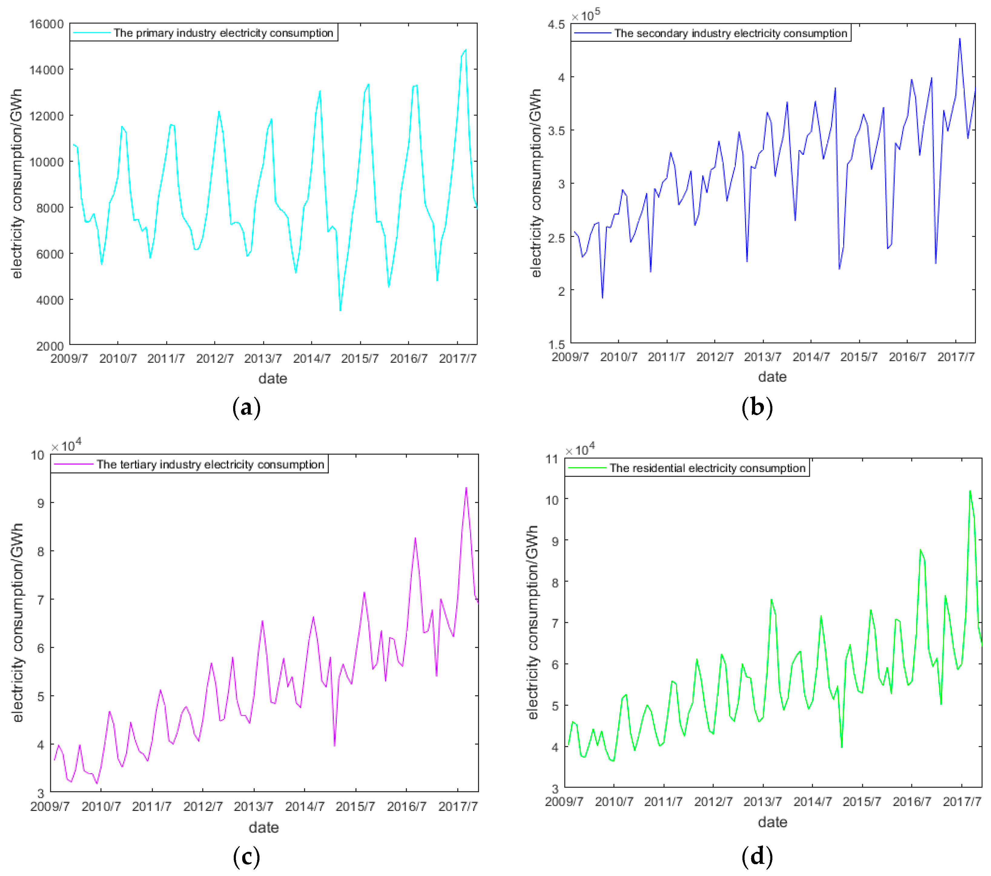
Figure 3.
(a) EEMD decomposition of monthly the primary industrial electricity consumption; (b) EEMD decomposition of monthly the secondary industrial electricity consumption; (c) EEMD decomposition of monthly the tertiary industrial electricity consumption; (d) EEMD decomposition of monthly the residential electricity consumption.

Figure 4.
(A) Diverse serial verification set mean absolute percentage error (MAPE) for primary industries electricity for different number of trees; (B) Diverse serial verification set MAPE for secondary industries electricity for different number of trees; (C) Diverse serial verification set MAPE for tertiary industries electricity for different number of trees; (D) Diverse serial verification set MAPE for residential electricity for different number of trees.
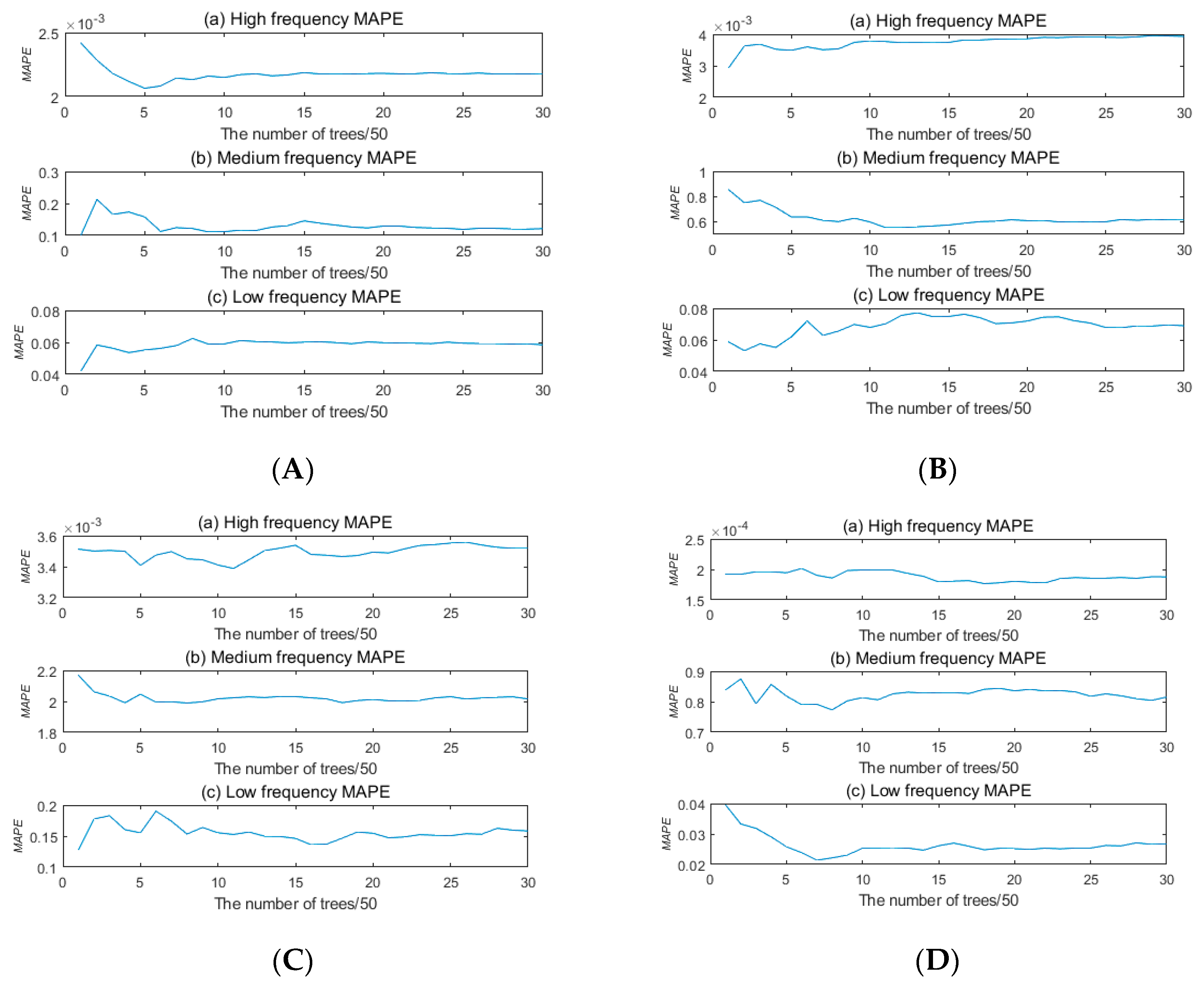
Figure 5.
(a) Fitting situation of monthly the primary industrial electricity consumption; (b) Fitting situation of monthly the secondary industrial electricity consumption; (c) Fitting situation of monthly the tertiary industrial electricity consumption; (d) Fitting situation of monthly the residential electricity consumption.
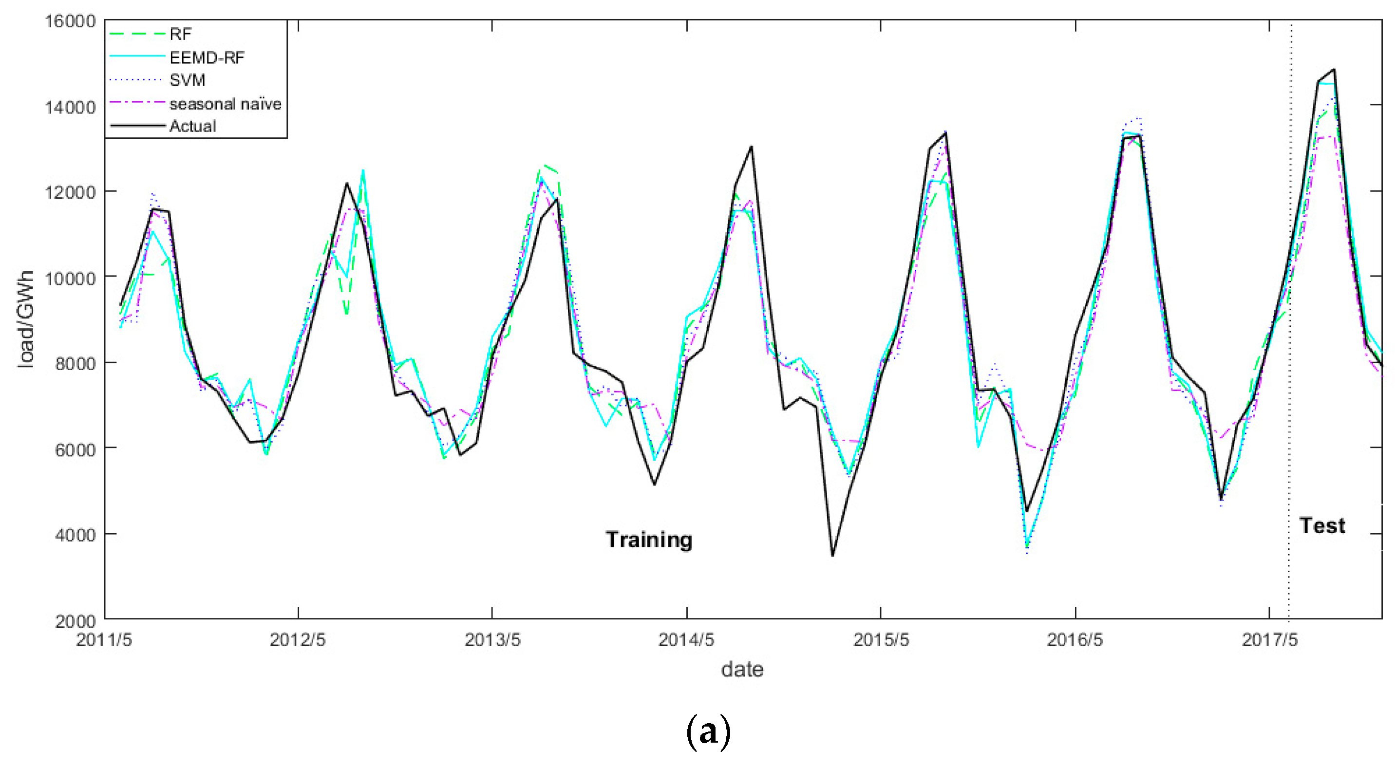

Table 1.
The forecast error of the primary, secondary and tertiary industries and residential electricity.
Table 1.
The forecast error of the primary, secondary and tertiary industries and residential electricity.
| Date | RF | SVM | Seasonal Naïve | EEMD+RF | |||||
|---|---|---|---|---|---|---|---|---|---|
| MAE/GWh | MAPE/% | MAE/GWh | MAPE/% | MAE/GWh | MAPE/% | MAE/GWh | MAPE/% | ||
| primary industry | June 2017 | 759.01 | 6.32 | 932.42 | 7.77 | 1219.64 | 10.16 | 178.52 | 1.49 |
| July 2017 | 885.42 | 6.09 | 839.29 | 5.77 | 1325.85 | 9.12 | 35.26 | 0.24 | |
| August 2017 | 826.59 | 5.57 | 628.12 | 4.23 | 1562.18 | 10.53 | 360.82 | 2.43 | |
| September 2017 | 336.60 | 3.11 | 230.92 | 2.14 | 317.48 | 2.94 | 560.39 | 5.19 | |
| October 2017 | 229.35 | 2.73 | 39.85 | 0.47 | 298.55 | 3.55 | 348.28 | 4.14 | |
| November 2017 | 17.89 | 0.23 | 36.37 | 0.46 | 241.46 | 3.06 | 310.50 | 3.93 | |
| average | 509.14 | 4.01 | 451.16 | 3.47 | 827.53 | 6.56 | 298.96 | 2.90 | |
| Secondary industry | June 2017 | 10,153.86 | 2.66 | 8146.92 | 2.13 | 19,551.72 | 5.11 | 3854.71 | 1.01 |
| July 2017 | 36,299.22 | 8.32 | 17,527.41 | 4.02 | 38,641.13 | 8.86 | 12,005.20 | 2.75 | |
| August 2017 | 18,760.53 | 4.82 | 11,782.69 | 3.03 | 9453.57 | 2.43 | 6522.62 | 1.68 | |
| September 2017 | 25,011.87 | 7.31 | 4318.14 | 1.26 | 16,010.54 | 4.68 | 6794.00 | 1.99 | |
| October 2017 | 13,456.31 | 3.69 | 13,432.03 | 3.68 | 10,273.23 | 2.81 | 11,723.03 | 3.21 | |
| November 2017 | 13,253.66 | 3.40 | 13,077.42 | 3.35 | 13,394.27 | 3.43 | 8633.36 | 2.21 | |
| average | 19,489.24 | 5.03 | 11,380.77 | 2.91 | 17,887.41 | 4.55 | 8255.49 | 2.14 | |
| Tertiary industry | June 2017 | 500.59 | 0.71 | 1745.41 | 2.49 | 6995.11 | 9.97 | 393.32 | 0.56 |
| July 2017 | 628.84 | 0.75 | 2678.48 | 3.19 | 9759.58 | 11.62 | 455.03 | 0.54 | |
| August 2017 | 349.02 | 0.37 | 2213.77 | 2.38 | 10,524.40 | 11.30 | 919.70 | 0.99 | |
| September 2017 | 99.37 | 0.12 | 1034.56 | 1.24 | 8814.73 | 10.56 | 281.07 | 0.34 | |
| October 2017 | 445.60 | 0.63 | 1321.19 | 1.87 | 7861.93 | 11.11 | 1521.72 | 2.15 | |
| November 2017 | 1619.15 | 2.36 | 2096.29 | 3.05 | 5426.42 | 7.90 | 1878.78 | 2.73 | |
| average | 607.10 | 0.82 | 1848.28 | 2.37 | 8230.36 | 10.41 | 908.27 | 1.22 | |
| Residential | June 2017 | 511.08 | 0.85 | 191.98 | 0.32 | 4150.09 | 6.92 | 136.92 | 0.23 |
| July 2017 | 1716.82 | 2.37 | 1808.31 | 2.50 | 5180.11 | 7.15 | 200.42 | 0.28 | |
| August 2017 | 10,646.75 | 10.43 | 6006.67 | 5.88 | 14,459.13 | 14.16 | 7968.42 | 7.80 | |
| September 2017 | 7485.38 | 7.85 | 4537.75 | 4.76 | 10,017.71 | 10.51 | 3856.98 | 4.05 | |
| October 2017 | 1065.12 | 1.55 | 2274.33 | 3.30 | 5572.24 | 8.10 | 705.25 | 1.02 | |
| November 2017 | 1161.40 | 1.81 | 823.43 | 1.28 | 4785.48 | 7.46 | 404.79 | 0.63 | |
| average | 3764.43 | 4.14 | 2607.08 | 3.01 | 7360.79 | 9.05 | 2212.13 | 2.33 | |
Table 2.
Six months’ electricity forecast for each method/GWh.
| Date | Orig | RF | MAE | MAPE/% | SVM | MAE | MAPE/% | Snaïve | MAE | MAPE/% | EEMD-RF | MAE | MAPE/% |
|---|---|---|---|---|---|---|---|---|---|---|---|---|---|
| June 2017 | 524,442 | 513,518 | 10,923 | 2.08 | 532,349 | 7907 | 1.51 | 492,525 | 31,917 | 6.09 | 526,236 | 1794 | 0.34 |
| July 2017 | 607,242 | 567,712 | 39,530 | 6.51 | 590,055 | 17,187 | 2.83 | 552,336 | 54,907 | 9.04 | 592,323 | 14,919 | 2.46 |
| August 2017 | 599,108 | 568,525 | 30,583 | 5.1 | 603,907 | 4799 | 0.8 | 563,109 | 35,999 | 6.01 | 595,088 | 4020 | 0.67 |
| September 2017 | 531,682 | 499,621 | 32,061 | 6.03 | 531,793 | 111 | 0.02 | 496,522 | 35,160 | 6.61 | 534,145 | 2463 | 0.46 |
| October 2017 | 512,995 | 498,258 | 14,738 | 2.87 | 528,296 | 15,301 | 2.98 | 488,989 | 24,006 | 4.68 | 523,040 | 10,045 | 1.96 |
| November 2017 | 531,016 | 518,202 | 12,814 | 2.41 | 546,499 | 15,484 | 2.92 | 507,168 | 23,848 | 4.49 | 542,461 | 11,445 | 2.16 |
Table 3.
Six months’ electricity consumption combined forecasting for the whole society/GWh.
| Date | Primary Industry | Secondary Industry | Tertiary Industry | Residential | Pred | Orig | MAE | MAPE/% |
|---|---|---|---|---|---|---|---|---|
| June 2017 | 11,587 | 387,474 | 69,039 | 59,778 | 527,878 | 524,442 | 3436 | 0.66 |
| July 2017 | 14,210 | 425,028 | 81,535 | 72,450 | 593,224 | 607,242 | 14,018 | 2.31 |
| August 2017 | 14,225 | 400,253 | 90,895 | 93,865 | 599,237 | 599,108 | 129 | 0.02 |
| September 2017 | 11,206 | 348,348 | 82,307 | 90,031 | 531,892 | 531,682 | 209 | 0.04 |
| October 2017 | 8652 | 377,706 | 69,236 | 68,610 | 524,204 | 512,995 | 11,208 | 2.18 |
| November 2017 | 8128 | 400,536 | 69,901 | 64,418 | 542,984 | 531,016 | 11,968 | 2.25 |
Table 4.
DM test of different models.
| DM-MAE | DM-MAPE | |||||||
|---|---|---|---|---|---|---|---|---|
| Primary | Secondary | Tertiary | Residential | Primary | Secondary | Tertiary | Residential | |
| RF | 1.968 | 2.149 | 2.155 | 1.700 | 1.987 | 2.408 | 2.054 | 1.856 |
| SVM | 1.977 | 2.687 | 2.284 | 1.653 | 2.015 | 2.741 | 2.368 | 1.743 |
| snaïve | 1.950 | 1.968 | 5.502 | 2.629 | 2.090 | 1.972 | 9.222 | 5.181 |
© 2018 by the authors. Licensee MDPI, Basel, Switzerland. This article is an open access article distributed under the terms and conditions of the Creative Commons Attribution (CC BY) license (http://creativecommons.org/licenses/by/4.0/).
Share and Cite
MDPI and ACS Style
Liu, D.; Sun, K.; Huang, H.; Tang, P. Monthly Load Forecasting Based on Economic Data by Decomposition Integration Theory. Sustainability 2018, 10, 3282. https://doi.org/10.3390/su10093282
AMA Style
Liu D, Sun K, Huang H, Tang P. Monthly Load Forecasting Based on Economic Data by Decomposition Integration Theory. Sustainability. 2018; 10(9):3282. https://doi.org/10.3390/su10093282
Chicago/Turabian StyleLiu, Da, Kun Sun, Han Huang, and Pingzhou Tang. 2018. "Monthly Load Forecasting Based on Economic Data by Decomposition Integration Theory" Sustainability 10, no. 9: 3282. https://doi.org/10.3390/su10093282
Note that from the first issue of 2016, this journal uses article numbers instead of page numbers. See further details here.