Comparing the Hydrological Responses of Conceptual and Process-Based Models with Varying Rain Gauge Density and Distribution

Abstract

Precipitation provides the most crucial input for hydrological modeling. However, rain gauge networks, the most common precipitation measurement mechanisms, are sometimes sparse and inadequately distributed in practice, resulting in an imperfect representation of rainfall spatial variability. The objective of this study is to analyze the sensitivity of different model structures to the different density and distribution of rain gauges and evaluate their reliability and robustness. Based on a rain gauge network of 20 gauges in the Jinjiang River Basin, south-eastern China, this study compared the performance of two conceptual models (the hydrologic model (HYMOD) and Xinanjiang) and one process-based distributed model (the water and energy transfer between soil, plants and atmosphere model (WetSpa)) with different rain gauge distributions. The results show that the average accuracy for the three models is generally stable as the number of rain gauges decreases but is sensitive to changes in the network distribution. HYMOD has the highest calibration uncertainty, followed by Xinanjiang and WetSpa. Differing model responses are consistent with changes in network distribution, while calibration uncertainties are more related to model structures.

1. Introduction

Precipitation is one of the most crucial inputs in catchment runoff modeling and measuring rainfall is essential for determining hydrological catchment response [1,2]. However, because precipitation is generated by extremely complicated, non-linear, and sensitive atmospheric physical process [3], it shows highly spatial and temporal variability at the basin scale [4,5,6,7].

Due to the importance of precipitation in modeling, prior work has evaluated the effect of uncertainty in precipitation on the response of simulated streams in hydrological models. Wilson et al. [8] found that peak runoff, total runoff volume, and peak timing are considerably influenced by the spatial distribution and precision of rainfall measurements. Singh [9] provided a detailed literature review on the influence of spatial–temporal variability in hydrological factors on rainfall runoff modeling. Sun et al. [10] found that runoff prediction errors at the catchment scale were significantly related to the representation of rainfall data spatial variability. Shen et al. [11] showed that noticeable uncertainty in stream flow and non-point source pollution modeling was caused by spatial rainfall uncertainty obtained from different precipitation interpolation methods.

Traditionally, there are three mechanisms for measuring or observing precipitation: rain gauges, weather radar, and satellite-based sensors [12,13,14]. Rain gauge networks remain the most common method for measuring precipitation [15,16,17] due to their higher accuracy in representing rainfall at their respective locations [18,19] and longer recording period for investigating long-term rainfall runoff processes [20]. Because a rain gauge is a point measurement for precipitation, representing rainfall spatial variability must be affected by the density and distribution of rain gauge networks. To address this relationship, Pardo-Igúzquiza [21] tried to optimize the rain gauge distribution and quantity in a given catchment. Chen et al. [22] proved that more pluviometers distributed in a catchment resulted in higher precision in areal precipitation calculation. Xu et al. [23] and Girons Lopez et al. [24] found there is a threshold value of rain gauge density, before which the presentation of rainfall improves significantly with increasing rain gauge numbers.

Significant early research focused on the effect of density and distribution of rain gauge networks on catchment modeling. However, most were only concerned with the impact of density. Michaud and Sorooshian [25] showed that poor rain gauge densities caused an inadequate simulation of flood peak in a midsized semi-arid catchment. Chaplot et al. [26] selected rain gauges with a certain empirical distribution. Andreassian et al. [27], Anctil et al. [28], and Xu et al. [23] randomly selected several subsets of different numbers of gauges to achieve the same level of rain gauge density and evaluated the relationship between density and modeling results. Similarly, Drogue and Khediri [29] employed approximately 100 subsets with the same number of rain gauges and used the mean average of rainfall data for their evaluated.

In the study of Bardossy and Das [30], distributions of rain gauges with different densities were obtained from an optimization algorithm. Some studies have considered pluviometer density and distribution at the same time [31], while other researchers have investigated the effect of udometer distribution on conceptual models [27,29,32]. These studies have evaluated the individual responses of different process-based models [26,31], compared a couple of models [33], and even applied a neural network to rainfall-runoff modeling [28]. However, a comprehensive comparison of the performances of different models impacted by different rain gauge network distributions, especially networks with varying numbers of gauges, has yet to be presented.

Identifying the effect of different rain gauges’ distribution on the hydrological response of conceptual and process-based models will be helpful in (1) optimizing rain gauge networks and (2) selecting hydrological models for a given basin. Therefore, this study aims to advance the discipline by comparing the impact of rain gauge distribution on typical conceptual and process-based distributed models. Furthermore, the potential influence of uncertainty in model calibrations is investigated. The paper is organized as follows: Section 2 introduces the study area, datasets, applied models and design scenarios. Section 3 provides the simulation results in two parts: for the whole validation period and a typical month within the validation period. Section 4 discusses the results and compares them with previous research. Section 5 provides the study conclusions.

2. Materials and Methods

2.1. Study Area

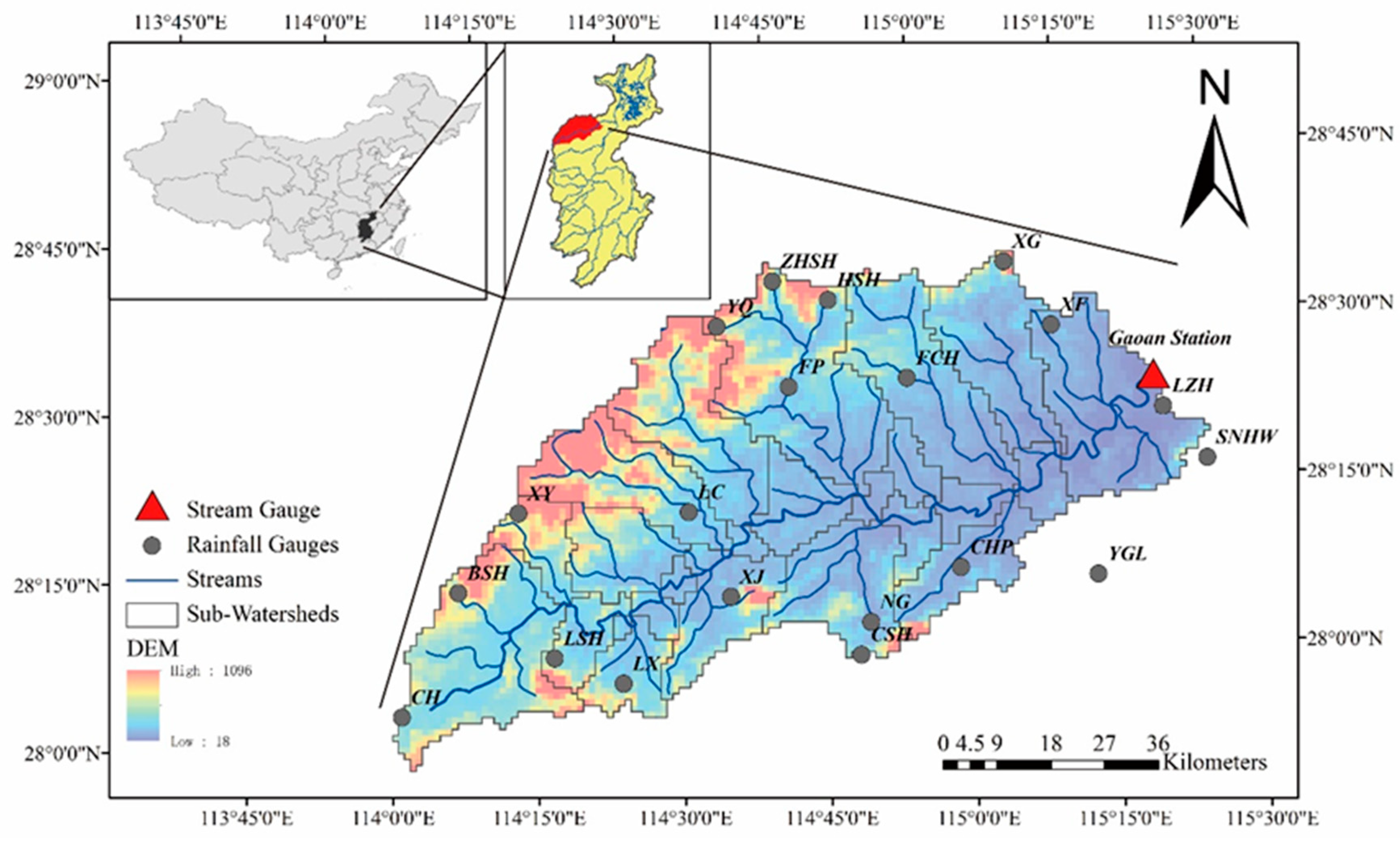
The Jinjiang River Basin is located in the north-west Ganjiang River Basin, China, with a drainage area of 6215 km² above the Gaoan hydrological station (Figure 1). The elevation of the catchment is higher in the north-west, where most tributaries of the Jinjiang River originate, ranging from 18 to 1096 m above sea level. The Jinjiang River Basin is located in the subtropical region with a warm and humid climate and receives approximately 1300–2100 mm of precipitation per year, with average runoff reaching about 184 m³/s at Gaoan station based on measured data. As the second largest tributary of the Ganjiang River, the Jinjiang River flows into the Ganjiang River about 30 km above Nanchang City, the capital city of Jiangxi Province, China. No controlled reservoirs have been built on the main stream of the Jinjiang River, resulting in a direct threat to Nanchang City during flood periods.

2.2. Datasets

Daily precipitation data from 20 rain gauges and observed streamflow data from the Gaoan hydrological station for 2008–2013 were provided by the Jiangxi Hydrological Bureau. The distribution of the pluviometers with their names and location of the Gaoan hydrological station are shown in Figure 1. The Thiessen polygon method [34] was used to interpolate the recorded rain data in the sub-basin areas.

Other meteorological data, including temperature, wind speed, relative humidity, and solar radiation, was obtained from the China Meteorological Assimilation Driving Datasets for the SWAT (Soil and Water Assessment Tool) model (CMADS) version 1.1 [35,36]. The CMADS datasets were developed based on the China Meteorological Assimilation Land Data Assimilation System (CLADS) with a temporal resolution of 1 day and spatial resolution of 0.25° × 0.25° [37]. The datasets were tested in the Heihe River Basin, Manas River Basin, and Hunhe River Basin [37,38,39], demonstrating a reliable performance in reflecting the observed meteorological data for China.

The digital elevation map (DEM) was developed by the Data Center for Resources and Environment Sciences, Chinese Academy of Sciences (RESDC), at a resolution of 1 km × 1 km. Land-use data with the same resolution as the DEM for the basin in 2000 were developed by the Institute of Geographical Sciences and Natural Resources Research, Chinese Academy of Sciences. The 10 km × 10 km cell soil data and related soil physical data were gathered from the Institute of Soil Science, Chinese Academy of Sciences.

2.3. Models

In this study, three hydrological models were applied to quantify hydrologic responses. Each model was a typical representation of a different model type, ranging from conceptual to physically based: the hydrologic model (HYMOD) [40], Xinanjiang model (XAJ) [41], and water and energy transfer between soil, plants and atmosphere model (WetSpa) [42]. All three models were used as semi-distributed models with the same watershed subdivisions shown in Figure 1. Each model operated on every sub-watershed separately with the same parameters while the rainfall and meteorological data were unique. The outputs from upper sub-basins were used as the inputs to the following sub-basins. Total streamflow for the entire basin was generated through all sub-basins according to hydraulic connections using the Muskingum method. Observed daily rainfall, potential evapotranspiration and runoff data at the Gaoan station were used as input data for all three models. The WetSpa model required the DEM, land use, and soil type for the study area.

2.3.1. Hydrologic Model (HYMOD)

HYMOD is a watershed-scale conceptual rainfall-runoff model based on the probability-distributed theory introduced by Moore [40]. It has been used in several rainfall runoff modeling studies [43,44,45,46]. This model describes runoff generation using a rainfall excess model and two sets of linear tanks (one slow flow tank and three identical tanks for quick flow) to reflect the routing process. The five parameters used in HYMOD are provided in

Table 1. Hydrologic model (HYMOD), Xinanjiang model (XAJ), and water and energy transfer between soil, plants and atmosphere model (WetSpa) parameters.

Model	Parameter	Description	Range
HYMOD *	Alpha	Partitioning factor between quick and slow flow	0.60~0.99
	bexp	Degree of spatial variability of soil moisture capacity in the catchment	0.00~2.00
	Cmax (mm)	Maximum soil moisture capacity in the catchment	0.00~1000
	Rq (day)	Residence time of the linear quick flow tanks	0.00~0.99
	Rs (day)	Residence time of the linear slow flow tank	0.001~0.10
XAJ *	UM (mm)	Averaged soil moisture storage capacity of the upper layer	5~100
	LM (mm)	Averaged soil moisture storage capacity of the lower layer	50~300
	DM (mm)	Averaged soil moisture storage capacity of the deep layer	5~100
	B	Exponential of the distribution to tension water capacity	0~1
	Im (%)	Percentage of impervious and saturated areas in the catchment	0~0.1
	C	Coefficient of the deep layer	0.15
	Sm (mm)	Areal mean free water capacity of the surface soil layer	5~100
	Ex	Exponent of the free water capacity curve influencing the development of the saturated area	1.0~1.5
	Kg	Outflow coefficients of the free water storage to groundwater relationships	0.05~0.70
	Ki	Outflow coefficients of the free water storage to interflow relationships	Kg + Ki = 0.7~0.8
	Cg	Recession constants for groundwater storage	0.9~0.999
	Ci	Recession constants for lower interflow storage	0.05~0.95
	Cs	Recession constant in the lag and route method for routing through the channel system within each sub-basin	0.001~0.8
	L (day)	Lag in time empirical value	0~3
WetSpa *	Ki	Interflow scaling factor	0~10
	Kg (day−1)	Groundwater recession coefficient	0~0.05
	Ks	Initial soil moisture factor	0~2
	Ke	Correction factor for potential evapotranspiration	0~2
	Kgi (mm)	Initial groundwater storage	0~500
	Kgm (mm)	Groundwater storage scaling factor	0~2000
	Kt (°C)	Base temperature for snowmelt	−1~1
	Ktd (mm °C−1 day−1)	Temperature degree-day coefficient	0~10
	Krd (°C−1 day−1)	Rainfall degree-day coefficient	0~0.05
	Km	Surface runoff coefficient	0~5
	Kp (mm)	Rainfall scaling factor	0~500

* Parameter ranges for HYMOD from Moradkhani et al. [45]. Parameter ranges for XAJ from Li et al. [50] and Lü et al. [60]. The selection and range in parameters for WetSpa from Shafii et al. [61].

; schematics for its application can be found in prior work [44,46].

2.3.2. Xinanjiang Model (XAJ)

The XAJ model, developed by Zhao et al. [41,47], has been widely applied in rainfall runoff simulation, hydrologic forecasting, and other applications [48,49]. This model is more parameterized in describing the details of hydrological responses than HYMOD because it has three modules: three-layer evapotranspiration, runoff generation, and runoff routing [47,50]. XAJ describes the underlying surface of the study area as three vertical layers, uper, lower, and deep. Runoff generation, routing, and evaporation are separately performed in the three layers. Descriptions of the 15 parameters, and their ranges, are provided in Table 1; the calculation process is summarized in Li et al. [50].

2.3.3. Water and Energy Transfer Between Soil, Plants and Atmosphere Model (WetSpa)

WetSpa is a typical physically based distributed model initially proposed by Wang et al. [42] and further perfected and applied to simulating hydrological processes by many researchers [51,52,53,54]. In this model, hydrological processes include precipitation, evapotranspiration, interception, infiltration, surface runoff, depression storage, percolation, ground water drainage, and interflow. Water and energy balances are considered within horizontal grid cells and in four vertical layers, the canopy, root layer, transmission layer, and saturated zone. Therefore, the model accounts for the highly spatial variance in meteorological data, terrain, land cover, and soil across a catchment. Values of some parameters, such as permeability and evapotranspiration rate, in a single grid cell can be determined from a priori knowledge from land use and soil types. Global parameters still need to be calibrated; some are presented in Table 1.

2.3.4. Model Calibration and Validation

Calibration is a necessary procedure for all hydrological models before simulating catchment rainfall runoff. The three described models are calibrated against 2009–2011 observed daily streamflow data with a 1-year period (2008) for spin-up. The dynamically dimensioned search algorithm (DDS) [55] is used to optimize parameters for each model. The DDS algorithm is a heuristic global random search algorithm, in which the search is performed in all dimensions of the decision space and the number of dimensions is reduced as the search continues. This process makes the DDS a very efficient optimization algorithm, which has been successfully applied to simulating rainfall runoff and predicting hydrology [56,57]. With a total 1000 search iterations, the model parameters are optimized by maximizing the objective function, the Nash–Sutcliffe efficiency (NSE) [58], given by:

$$\mathrm{NSE}=1-\frac{{{\displaystyle \sum }}_{i=1}^N{(ob{s}_i-si{m}_i)}^2}{{{\displaystyle \sum }}_{i=1}^N{\left(ob{s}_i-\overline{obs}\right)}^2},$$

(1)

in which obs and sim are the observed and simulated daily runoff, respectively, $\overline{obs}$ is the mean value of observed runoff, i is the ith day, and N is the number of days. A value of 1 for NSE represents a perfect fit. Considering the equifinality in model calibration [59], each model is calibrated for 30 trials to achieve a better statistical representativeness of the results in the validation period.

The optimized parameter values from the calibration are used to model runoff for 2012–2013. The statistical criteria used to quantitatively evaluate model performance are relative bias (BIAS), reflecting the ability of recreating the water balance; the Pearson correlation coefficient (CC), which manifests the agreement between the simulated and the observed runoff; and NSE, as described above, which evaluates the goodness of the model results. The first two indexes are given by the following expressions:

$$\mathrm{BIAS}=\frac{{{\displaystyle \sum }}_{i=1}^N\left(si{m}_i-ob{s}_i\right)}{{{\displaystyle \sum }}_{i=1}^{N}ob{s}_i}\times 100\%,$$

(2)

$$\mathrm{CC}= \frac{\frac{1}{N}{{\displaystyle \sum }}_{i=1}^N\left(si{m}_i-\overline{sim}\right)\left(ob{s}_i-\overline{obs}\right)}{{\sigma }_{sim}{\sigma }_{obs}},$$

(3)

where, σ_sim and σ_obs are standard deviations of simulated and observed runoff series, $\overline{sim}$ is the average value of assumed runoff, and the other symbols are the same as defined for Equation (1). The perfect value for BIAS is 0; for CC it is 1. The standard deviation σ is calculated as follows:

$$\sigma =\sqrt{\frac{1}{N}{{\displaystyle \sum }}_{i=1}^N{\left(x_i-\overline{x}\right)}^2},$$

(4)

where, x_i is the ith value of observed or simulated daily runoff, $\overline{x}$ is the arithmetic average value of observed or simulated daily runoff, and the remaining symbols are the same as defined previously.

2.3.5. Scenario Settings

The correlations between rain data for a single gauge and streamflow data for Gaoan station are provided in

Table 2. Correlation between rain and streamflow data and gauge selection for different scenarios.

Gauge Name	CC_0 *	CC_1	CC_2	CC_3	20_C **	15_C	10_C	5_C	15_SW	15_SE	15_NW	15_NE	10_SW	10_SE	10_NW	10_NE	5_SW	5_SE	5_NW	5_NE
BSH	0.142	0.492	0.581	0.360	√ ***	√			√	√	√		√				√
CSH	0.131	0.496	0.532	0.328	√				√	√	√	√		√	√				√
CHP	0.139	0.548	0.575	0.363	√	√	√	√	√	√		√		√		√		√
CH	0.145	0.459	0.538	0.356	√	√	√	√	√	√	√	√	√	√		√	√			√
FCH	0.158	0.564	0.589	0.378	√	√	√	√		√	√	√			√	√
FP	0.140	0.538	0.574	0.403	√	√			√		√	√	√		√		√
HSH	0.143	0.478	0.568	0.365	√	√			√		√	√			√	√			√
LSH	0.151	0.512	0.589	0.376	√				√	√	√		√	√	√		√
LX	0.147	0.512	0.569	0.361	√	√	√		√	√	√		√	√				√
LZH	0.143	0.534	0.537	0.337	√	√	√	√	√	√	√	√	√	√		√	√			√
LC	0.143	0.562	0.584	0.355	√	√	√	√	√	√	√	√	√		√	√				√
NG	0.128	0.513	0.547	0.337	√	√	√		√	√		√	√	√				√
SNHW	0.136	0.523	0.547	0.346	√					√		√		√		√		√
XG	0.148	0.510	0.548	0.357	√	√	√				√	√			√	√			√	√
XY	0.151	0.497	0.592	0.386	√	√	√		√		√		√		√				√
XF	0.155	0.568	0.569	0.361	√	√				√	√	√				√				√
XJ	0.140	0.539	0.593	0.373	√	√			√	√			√
YGL	0.161	0.548	0.552	0.355	√					√		√		√		√
YQ	0.145	0.478	0.569	0.383	√	√	√		√	√	√	√		√	√			√	√
ZHSH	0.142	0.492	0.581	0.360	√	√			√	√	√		√				√

* CC_0, CC_1, CC_2, and CC_3 refer to the correlation between rain and streamflow data on the same day and after 1 day, 2 days, and 3 days delay; ** The number in front of the underline is the number of rain gauges used in the scenario and the letters followed by the underline refer to the direction of most rain gauges: C is central and SW, SE, NW, NE indicate south-west, south-east, north-west, and north-east, respectively; *** The ticks refer to the rain gauges selected in the named scenario.

. Notably, all rain gauges have higher relevance with runoff data with 1 day or 2 days delay, even for LZH, which is the nearest udometer to Gaoan station. However, not a single gauge is significantly related to the streamflow data, and the reverse is the same. To estimate the model uncertainties resulting from the accuracy of precipitation measurements, a total of 16 scenarios with varying rain gauge numbers and distributions are evaluated in this study. As presented in Table 2, rain gauge partition is described in terms of the direction that the barycenter selected udometer sets. Most rain gauges are distributed in one direction, while at least one rain gauge is set to the opposite direction to provide necessary rainfall spatial variety. According to the shape of Jinjiang River Basin, the directions are classified as central, north-east, north-west, south-east, and south-west. Given the five rain gauge distributions and four selected rain gauge quantities, i.e., 5, 10, 15, and 20, different pluviometer densities are defined in the study area. For each direction, rain gauges in scenarios with lower quantity are selected from those with higher quantity, i.e., 10 rain gauges in scenario 10_C are selected from those in scenario 15_C, while udometers in 10_SE are selected from those from 15_SE. Therefore, higher quantity scenarios contain all rain gauges in lower quantity scenarios in the same direction.

3. Results

Daily streamflow reproduction performance of the three models for 16 rain gauge scenarios during the validation period is investigated in two parts. In part I, general model performance during the entire validation period (1 January 2012 to 31 December 2013) is assessed using the statistical results from the evaluating indicators described in Section 2.3.4. In part II, model performance is discussed for a single month (June 2012) with a detailed daily flow hydrograph comparison.

3.1. Model Performance in the Calibration and Validation Period

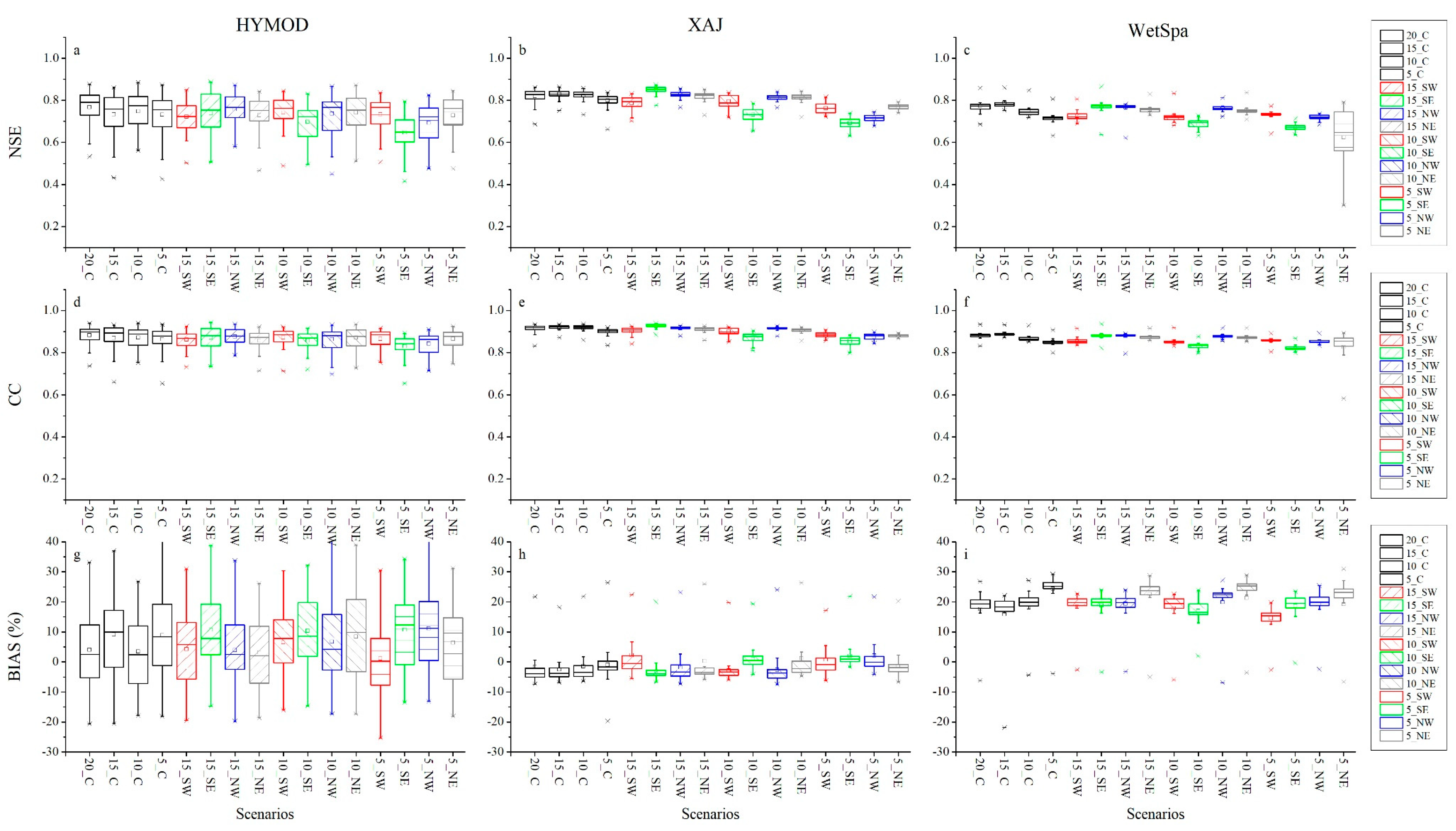
To compare model performance between HYMOD, XAJ, and WetSpa for the 16 rain gauge scenarios, the statistical criteria in the calibration and validation period are provided in

Table 3. HYMOD model performance in the calibration and validation periods.

Scenarios	Calibration									Validation
	Nash–Sutcliffe Efficiency (NSE)			CC			Relative bias (BIAS) (%)			NSE			CC			BIAS (%)
	Mean *	Q1 **	Q3 ***	Mean	Q1	Q3	Mean	Q1	Q3	Mean	Q1	Q3	Mean	Q1	Q3	Mean	Q1	Q3
20_C **	0.773	0.739	0.835	0.888	0.868	0.919	19.003	8.889	26.535	0.768	0.732	0.823	0.883	0.862	0.909	4.020	−4.890	12.174
15_C	0.735	0.674	0.815	0.870	0.856	0.915	22.206	12.316	33.722	0.735	0.676	0.815	0.871	0.855	0.916	9.154	−1.015	17.154
10_C	0.748	0.681	0.818	0.876	0.842	0.914	17.914	8.661	27.312	0.748	0.691	0.818	0.871	0.837	0.907	3.471	−6.971	11.868
5_C	0.751	0.695	0.823	0.876	0.852	0.917	20.961	9.556	32.543	0.732	0.677	0.799	0.864	0.845	0.901	8.857	−0.621	18.546
15_SW	0.734	0.666	0.797	0.869	0.836	0.901	17.086	5.113	27.538	0.723	0.670	0.775	0.861	0.834	0.888	4.292	−5.733	13.162
15_SE	0.739	0.685	0.828	0.870	0.833	0.918	25.110	14.905	32.557	0.738	0.675	0.829	0.871	0.835	0.914	10.662	2.633	18.726
15_NW	0.763	0.721	0.830	0.881	0.860	0.915	19.716	9.529	28.525	0.758	0.719	0.817	0.877	0.850	0.909	3.906	−2.408	12.315
15_NE	0.745	0.721	0.810	0.868	0.855	0.905	17.639	7.819	23.752	0.730	0.703	0.796	0.857	0.842	0.892	3.095	−7.043	11.833
10_SW	0.770	0.743	0.829	0.887	0.870	0.917	18.232	10.583	26.310	0.743	0.715	0.801	0.871	0.852	0.901	6.524	0.183	13.724
10_SE	0.742	0.689	0.814	0.871	0.851	0.907	24.799	13.924	34.437	0.698	0.634	0.751	0.858	0.834	0.888	10.390	1.893	19.676
10_NW	0.725	0.657	0.797	0.861	0.829	0.900	28.033	19.387	38.300	0.737	0.672	0.792	0.863	0.830	0.896	6.797	−2.554	15.573
10_NE	0.759	0.702	0.824	0.881	0.847	0.920	22.330	12.071	34.628	0.742	0.684	0.810	0.871	0.836	0.907	8.496	−2.363	20.696
5_SW	0.730	0.684	0.789	0.861	0.837	0.892	12.749	5.435	19.056	0.734	0.688	0.789	0.864	0.839	0.899	1.092	−7.768	7.817
5_SE	0.718	0.690	0.795	0.857	0.843	0.903	27.811	14.713	37.411	0.647	0.603	0.707	0.829	0.817	0.865	10.722	−0.366	18.679
5_NW	0.685	0.635	0.764	0.843	0.817	0.890	33.136	22.002	42.193	0.693	0.627	0.760	0.842	0.807	0.879	11.204	1.114	19.273
5_NE	0.747	0.716	0.817	0.872	0.855	0.911	20.740	8.448	29.119	0.729	0.683	0.802	0.866	0.836	0.897	6.427	−5.730	14.650

* Mean refers to the arithmetic average value; ** Q1 refers to the 1st quartile value; *** Q3 refers to the 3rd quartile value.

,

Table 4. XAJ model performance in the calibration and validation periods.

Scenarios	Calibration									Validation
	NSE			CC			BIAS (%)			NSE			CC			BIAS (%)
	Mean	Q1	Q3	Mean	Q1	Q3	Mean	Q1	Q3	Mean	Q1	Q3	Mean	Q1	Q3	Mean	Q1	Q3
20_C	0.805	0.796	0.832	0.899	0.893	0.913	14.042	8.603	14.491	0.821	0.809	0.842	0.914	0.910	0.926	−1.604	−5.024	−2.210
15_C	0.811	0.806	0.830	0.903	0.899	0.912	11.314	7.758	12.817	0.829	0.822	0.843	0.919	0.915	0.927	−2.446	−4.804	−1.964
10_C	0.812	0.811	0.831	0.905	0.903	0.914	12.109	8.325	12.440	0.823	0.816	0.840	0.917	0.915	0.927	−1.447	−4.769	−1.340
5_C	0.782	0.772	0.806	0.886	0.879	0.898	11.608	9.602	13.865	0.800	0.788	0.818	0.900	0.895	0.909	−0.904	−2.673	0.318
15_SW	0.791	0.787	0.818	0.893	0.887	0.906	15.946	11.028	14.928	0.787	0.773	0.812	0.900	0.898	0.915	2.202	−2.183	1.754
15_SE	0.827	0.821	0.843	0.911	0.907	0.919	10.877	8.629	11.750	0.848	0.843	0.861	0.926	0.924	0.934	−2.908	−4.482	−2.859
15_NW	0.801	0.791	0.821	0.897	0.889	0.907	12.844	8.187	14.691	0.827	0.822	0.837	0.915	0.914	0.922	−1.877	−4.747	−1.036
15_NE	0.804	0.800	0.824	0.899	0.895	0.908	14.371	9.922	13.640	0.815	0.813	0.831	0.908	0.907	0.917	0.270	−4.015	−2.031
10_SW	0.783	0.768	0.803	0.887	0.879	0.898	9.549	7.081	10.841	0.795	0.774	0.823	0.900	0.890	0.916	−2.834	−4.469	−2.588
10_SE	0.804	0.787	0.824	0.898	0.889	0.910	15.185	11.525	17.249	0.731	0.712	0.755	0.872	0.858	0.887	0.933	−0.783	1.984
10_NW	0.795	0.789	0.814	0.893	0.889	0.903	15.176	10.870	16.050	0.810	0.806	0.821	0.913	0.913	0.919	−2.662	−5.331	−2.555
10_NE	0.809	0.806	0.833	0.901	0.899	0.915	14.417	10.269	14.019	0.810	0.806	0.825	0.904	0.902	0.913	1.236	−3.459	0.220
5_SW	0.700	0.681	0.722	0.838	0.826	0.850	15.713	11.123	17.517	0.764	0.740	0.783	0.883	0.875	0.893	0.763	−2.717	1.300
5_SE	0.818	0.809	0.838	0.906	0.900	0.917	17.197	14.761	18.063	0.692	0.675	0.710	0.853	0.840	0.869	2.038	0.162	1.821
5_NW	0.765	0.765	0.794	0.880	0.875	0.893	22.487	18.422	20.941	0.715	0.705	0.728	0.876	0.866	0.887	2.164	−1.466	1.757
5_NE	0.767	0.752	0.786	0.876	0.867	0.887	13.463	11.373	14.930	0.769	0.761	0.778	0.881	0.876	0.885	−1.531	−2.978	−0.898

and

Table 5. WetSpa model performance in the calibration and validation periods.

Scenarios	Calibration									Validation
	NSE			CC			BIAS (%)			NSE			CC			BIAS (%)
	Mean	Q1	Q3	Mean	Q1	Q3	Mean	Q1	Q3	Mean	Q1	Q3	Mean	Q1	Q3	Mean	Q1	Q3
20_C	0.736	0.726	0.738	0.873	0.867	0.877	37.173	37.888	41.076	0.773	0.761	0.781	0.883	0.877	0.886	17.625	17.879	20.637
15_C	0.739	0.723	0.737	0.874	0.867	0.873	32.699	35.497	37.932	0.787	0.773	0.789	0.890	0.883	0.890	15.920	16.891	20.185
10_C	0.722	0.707	0.724	0.870	0.862	0.870	38.330	39.602	42.736	0.751	0.733	0.756	0.870	0.860	0.872	18.092	18.701	21.349
5_C	0.661	0.645	0.664	0.839	0.831	0.843	38.849	38.624	41.266	0.716	0.709	0.722	0.850	0.845	0.854	24.333	24.460	26.359
15_SW	0.702	0.678	0.709	0.860	0.854	0.863	35.191	35.874	38.798	0.726	0.713	0.734	0.856	0.847	0.860	18.333	18.784	21.025
15_SE	0.726	0.722	0.733	0.869	0.866	0.874	36.658	36.733	39.689	0.772	0.765	0.778	0.882	0.878	0.885	18.837	18.737	21.060
15_NW	0.703	0.701	0.714	0.860	0.860	0.866	39.389	38.772	41.964	0.767	0.767	0.775	0.880	0.880	0.885	19.420	18.159	21.041
15_NE	0.734	0.726	0.737	0.874	0.869	0.877	39.874	40.299	42.661	0.756	0.747	0.761	0.874	0.867	0.877	22.542	22.429	25.017
10_SW	0.727	0.713	0.731	0.865	0.860	0.869	34.026	34.220	37.596	0.723	0.710	0.726	0.853	0.846	0.855	17.859	17.903	20.967
10_SE	0.706	0.696	0.715	0.864	0.859	0.867	38.548	37.182	40.586	0.687	0.676	0.702	0.831	0.824	0.839	17.035	15.835	19.296
10_NW	0.692	0.675	0.696	0.855	0.848	0.859	43.935	45.957	47.672	0.763	0.757	0.770	0.879	0.874	0.882	19.956	21.523	22.941
10_NE	0.726	0.710	0.726	0.869	0.862	0.870	36.227	38.853	41.945	0.754	0.744	0.755	0.874	0.868	0.876	21.285	23.789	25.982
5_SW	0.647	0.650	0.655	0.814	0.817	0.819	31.600	31.541	33.406	0.733	0.730	0.737	0.858	0.856	0.860	14.480	13.847	16.308
5_SE	0.718	0.704	0.722	0.872	0.866	0.875	40.607	40.459	42.972	0.673	0.663	0.679	0.823	0.816	0.826	18.699	18.012	21.161
5_NW	0.651	0.635	0.654	0.837	0.829	0.840	46.650	47.065	50.304	0.720	0.714	0.729	0.854	0.848	0.857	19.128	18.735	21.488
5_NE	0.615	0.617	0.666	0.799	0.811	0.831	36.948	36.992	43.946	0.624	0.564	0.746	0.827	0.834	0.868	19.305	21.478	24.260

. Boxplots for the validation period are shown in Figure 2.

Table 3 indicates stable NSE and CC values between the calibration and validation periods for HYMOD in all 16 scenarios. However, there is an clear improvement in the BIAS value from the calibration to validation period. XAJ shows similar behavior (Table 4). WetSpa shows a slight improvement in NSE and CC values in most scenarios (Table 5).

Figure 2a–c illustrates the accuracy of the streamflow simulations, as indicated by NSE. Generally, metrics for the validation period are acceptable for all three models despite different pluviometer selection scenarios; average NSE values are greater than 0.6. In more detail, results for XAJ are better than those for HYMOD and WetSpa, and the latter two are comparable in most scenarios. Notably, there are discrepancies between the NSE values for the three models. Interquartile ranges for HYMOD are significantly larger than those for XAJ, followed by those for WetSpa, which has the narrowest interquartile NSE range. WetSpa shows the best stability in model performance in every calibration trial, while HYMOD has the largest uncertainty.

When rain gauge selections are taken into consideration, results for all three models perform consistently. With the reduction in rain gauge numbers (scenario 20_C, 15_C, 10_C and 5_C), the mean NSE values for all models show lower variability. The NSE amplitudes for HYMOD and XAJ are rather small, showing robustness for a simple decline in the quantity of udometers. In contrast, the values for WetSpa show greater sensitivity toward changes in rain gauge quantity.

The impacts of the spatial distribution of rain gauges show similar trends in terms of NSE metrics for all models. With the same number of rain gauges (15), all models in scenario 15_SE and 15_NW perform comparably with those in 15_C. However, the accuracy of the results in scenario 15_SW is generally lower. Unexpectedly, model performances for 10_SE and 5_SE are poorest among scenarios with the same number of rain gauges. Similarly, model performance worsens with a decrease in rain gauges from 15 to 5 when the rain gauges are concentrated in the north-west part of the basin (scenarios 15_NW, 10_NW, and 5_NW). Furthermore, variations in the number of rain gauges concentrated in the south-west and north-east has few impacts on streamflow simulations, except for WetSpa in scenario 5_NE, which shows a dramatic reduction in both average and variation in NSE values. Similar results are found for the CC values, as illustrated in Figure 2d–f.

Figure 2g–h shows the ability of the three models to recreate the water balance for the 16 rain gauge scenarios. Generally, HYMOD and XAJ exhibit better performance in water balance simulations; HYMOD overestimates and XAJ underestimates the average within about 5%. WetSpa poorly estimates water balance with a BIAS of approximately 20%. Interquartile ranges for BIAS indicate that WetSpa has most stable model performance, while HYMOD has the lowest under multiple calibrations, as indicated previously.

3.2. Monthly Analysis for 2012

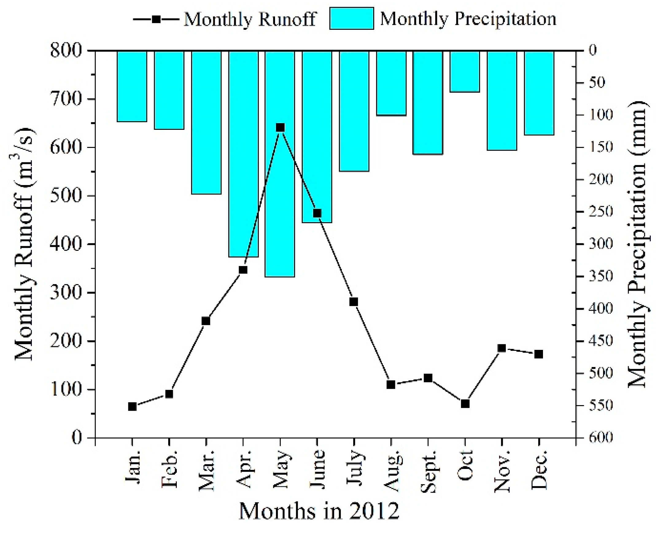
Monthly performance is another important mechanism for comparing models’ responses due to different rain gauge distributions. Figure 3 illustrates the monthly average runoff and precipitation in the Jinjiang River Basin. Clearly, the wet season in 2012 ranges from March to July, resulting in a flood season with average flow above 200 m³/s. However, dry seasons are not particularly dry; most months, except for August and October, have average precipitation over 100 mm per month.

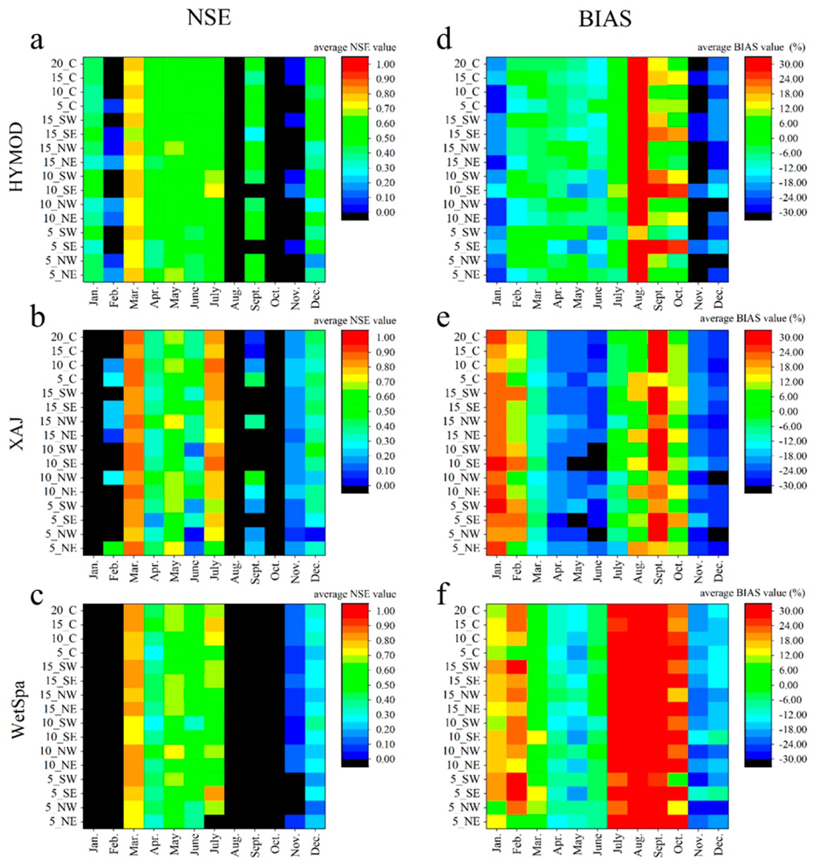
Monthly comparisons for HYMOD, XAJ, and WetSpa are shown in Figure 4. As shown in Figure 4a–c, all three models tend to simulate streamflow in the flood season better, but poorly reproduce runoff in the dry season, especially in August and October. Specifically, HYMOD shows better adaptability than XAJ and WetSpa, achieving acceptable NSE values in more months, especially in January and September. However, WetSpa performs worse than the other models in March, May, July, and November. In addition, HYMOD monthly performances show no distinct trends indicating an impact of rain gauge distributions. XAJ demonstrates higher usability in the flood season. However, it is more likely to be affected by the distribution of rain gauges. June, for example, has the highest NSE value (0.50) in scenario 15_SE, but the lowest NSE value (0) in 5_NW. Finally, WetSpa only achieves acceptable results in the flood season. NSE values in the dry season are no higher than 0.1, except for December, in which NSE values are about 0.3.

The overall deviations for all three models vary significantly from month to month (Figure 4d–f). Of the three models, HYMOD generates relatively accurate overall estimates in most months. However, it overestimates total flood volume in August and underestimates total flood volume in January, November, and December. XAJ produces results that vary between overestimates and underestimates. The WetSpa model achieves the best performance in March, but produces more than 30% overestimates from July to October, which confirms the results in Figure 4c.

3.3. Model Performance in June 2012

To investigate the performance of three models based on data precision for different precipitation values, daily time series of the simulated and observed hydrographs in a typical wet season month in the Jinjiang River basin (June 2012) are compared. June 2012 has two complete flood peaks, and the two peak flows are neither too high nor too low. Therefore, analyzing model performance in June 2012 is appropriate.

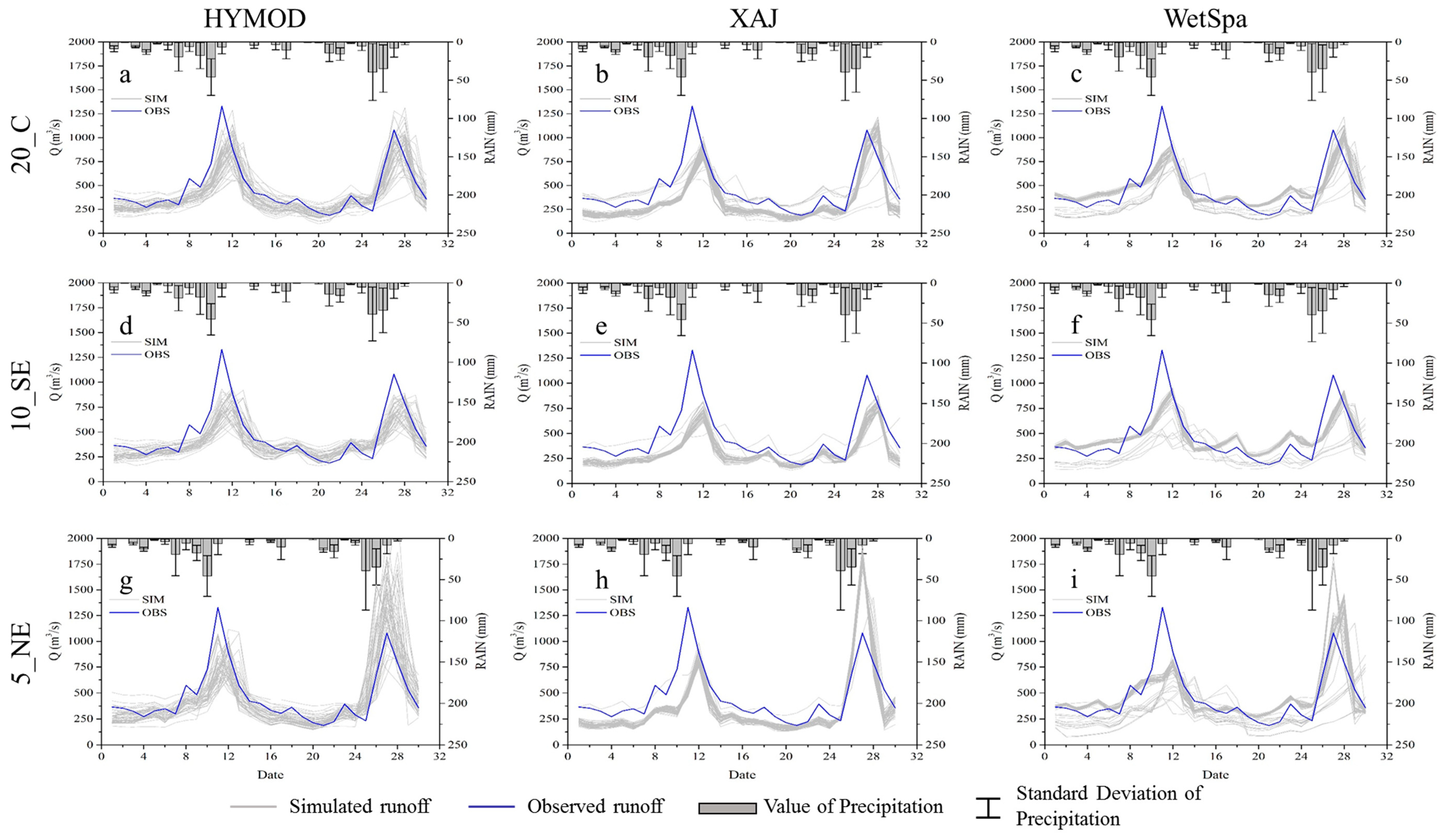
As presented in Figure 5, the accumulative precipitation in June 2012 ranges from 187.1 mm to 355.3 mm. The rain center is located in the central area of the basin captured by rain gauge LC. Therefore, three scenarios, 20_C as a benchmark, 10_SE absent LC, and 5_NE with LC (see Table 2), are investigated as LC presence could be a critical factor affecting runoff modeling.

Figure 6a indicates that in scenario 20_C, HYMOD results generally agree with daily observed streamflow in June 2012. However, hydrographs in every trial range widely compared with XAJ (Figure 6b) and WetSpa (Figure 6c). XAJ and WetSpa misrepresent the first peak flow in June, while capturing the second. XAJ underestimates the lower streamflow, while WetSpa slightly overestimates them.

Absent the key rain gauge LC in scenario 10_SE (Figure 6d–f), the standard deviations in measured rain data on 25 June 2012 are clearly smaller than in 20_C. The remaining rain gauges do not correctly reflect the spatial variability in actual precipitation for the entire basin. All three models underestimate the second peak flow that they precisely captured in 20_C. For 5_NE, all models overestimate the second peak flow as the rainfall data from LC are assumed to represent the areal rainfall input from most sub-watersheds (Figure 6g–i).

Meanwhile, variations in simulated second peak flow for WetSpa increase notably and the simulated runoff time series can be divided into three groups. Most hydrographs in one group tend to appreciably overestimate the second peak flow. While those in another group tend to significantly overestimate the second peak flow, e.g., XAJ. The remainder in the third group tend to miss the second peak flow.

4. Discussion

The sensitivity of HYMOD, XAJ, and WetSpa models is compared to characterize the spatial distribution of rainfall in a medium scale semi-humid watershed in southeast China. The NSE, CC, and BIAS values for 16 rain gauge distribution scenarios are used to assess the performance of hydrological models with varying rain gauge deployment locations. The HYMOD and XAJ models can be regarded as representative conceptual models with different complexity, while the WetSpa model is considered a typical process-based distributed model.

4.1. Influence of Rain Gauge Distribution

For all three models, runoff varied slightly with a decreasing number of rain gauges (from 20 to 5). This result differs from the previous studies of Andreassian et al. [27] and Xu et al. [23], which showed that model efficiency declines with loss of rainfall spatial knowledge. However, it agrees with Chaplot et al. [26], who found that model performance remains stable despite decreasing gauge concentration. One explanation is that former studies used lumped hydrological models that applied average surface rainfall as input while the SWAT used in Chaplot et al. [26] is a distributed model that takes advantage of rainfall data interpolated into each sub-catchment. In this study, all three models are applied as semi-distributed models, and thus rainfall spatial variety is captured with a limited number of rain gauges. While all models are able to cope with a restricted number of rain gauges, their distribution is more likely to result in uncertainty in simulated streamflow. These results suggest that appropriate rain gauge configuration is of higher importance than the number or density of rain gauges in a certain catchment.

4.2. Comparing Different Model Structures

Because all three models are regarded as semi-distributed models that operate on sub-basins with distributed rainfall data, differences in simulated runoff between them is likely derived from model complexity and the rationality of parameterization. The general model precision and uncertainty performance in scenario 20_C is consistent with multiple studies [52,61,62,63,64].

The factor leading to larger uncertainty in model calibration for HYMOD and smaller uncertainty for WetSpa can be attributed to model structure complexity. In the model calibration process, optimization algorithms are supposed to reach optimal values. However, reaching the global optimal value requires significant computing resources and time. Therefore, most trials in the calibration period just reach local optimal values. It is possible that a higher complexity model structure could result in local optimal values closer to global optimal values according to the concept of equifinality introduced by Beven [59]. However, HYMOD has a simpler structure than XAJ and WetSpa with fewer parameters, leading to a parameter space consisting of fewer dimensions and fewer parameter combinations that can reach the ‘best’ performance, i.e., the global optimal value, during calibration. Most local optimal values are worse than the global optimal values, but the corresponding parameter sets are possibly reached during calibration. Therefore, HYMOD performance varies widely for each calibration trial.

Different performances in the water balance simulations are a more complex problem. As illustrated in Figure 2h, XAJ tends to underestimate total water volume in general. Sun et al. [65] reported similar results and concluded that underestimates of free water storage lead to underestimates of total water volume. In addition, WetSpa systematically overestimates total runoff volume. This behavior may be due to a consistent overestimate of low flows and an underestimate of high flows, where the total volume of low flows is higher than that of high flows (see Figure 4c,f,g).

4.3. Detailed Discussion on Model Performance

Finally, it is important to examine the inconsistent simulation of the two floods in June 2012. As illustrated in Figure 6, it is clear that observed streamflow is sensitive to rainfall; for example, small flood peaks on 8 and 18 June were obtained after relatively small rainfall events, showing that basin storage (including soil and groundwater) is rather limited and thus surface flow can be generated directly. When verifying the simulated flow from XAJ and WetSpa, however, responses to small rainfall events are systematically underestimated. While in the two major floods, the simulated streamflow increases and reaches the flood peaks with a one-day delay compared with the observed data, but decreases back to normal at the same day, or even earlier. Similar behavior appears in other flood simulations, as presented in

Table 6. Detailed model performances for sample floods in scenario 20_C.

Selected Flood			Total Average Rainfall (mm)	HYMOD			XAJ			WetSpa
Start Date	End Date	Actual Peak Flow (m3/s)		Delay 1 (day)	BIASp 2 (%)	BIASv 3 (%)	Delay (day)	BIASp (%)	BIASv (%)	Delay (day)	BIASp (%)	BIASv (%)
29 February 2012	13 March 2012	842	148.3	0	−4.9	−9.8	0	−6.5	−12.7	0	−2.5	−8.3
9 June 2012	14 June 2012	1330	74.3	1	−32.1	−21.1	1	−37.4	−33.3	1	−36.3	−21.3
25 June 2012	1 July 2012	1080	83.0	1	−12.2	−4.1	1	−2.7	−14.7	1	−7.0	−4.9
4 April 2013	9 April 2013	726	62.9	0	−9.8	−10.6	0	−12.1	−11.9	0	−9.2	−6.0
14 May 2013	21 May 2013	772	96.3	0	−11.2	1.8	0	−11.5	−8.6	1	−5.9	2.8

¹ Denotes the delay days that the simulated flood peak occurs in 30 trials minus the date of the observed flood peak; ² refers to the mean BIAS calculated using the simulated flood peak volume versus observed flood peak volume; ³ denotes the mean BIAS calculated using the simulated total flood volume versus observed total flood volume.

. These deviations are likely due to overestimating the water storage capacity of the basin. Hence, in the first flood period with rainfall concentrated in a single day, more precipitation turns into storage and generates streamflows with a longer delay, resulting in an average underestimation of −32.1%, −37.4%, and −36.3% in peak flow and −21.1%, −33.3%, and −21.3% in total volume for HYMOD, XAJ, and WetSpa, respectively (see Table 6). In the second flood period, with rainfall scattered over two days, precipitation in the first day fulfills the water storage and thus precipitation on the following day generates surface flow directly, resulting in a better reproduction of the second peak flow. The underestimation drops remarkably to −12.2%, −2.7%, and −7.0% in peak flow and −4.1%, −14.7%, and −4.9% in total volume (shown in Table 6). Such uncertainty derived from the model structure or model parameters needs to be addressed in further studies.

5. Conclusions

This study compared the performance and uncertainties of the HYMOD, XAJ, and WetSpa conceptual and process-based models with varying rain gauge numbers and distributions in the Jinjiang River Basin, China. Long time series, monthly, and daily performance was analyzed using several statistical indicators.

The results for all three models showed that a reduction in the number of rain gauges only resulted in worse performance when the rain gauge distribution was inhomogeneous. This observation demonstrates that appropriate rain gauge configuration is of greater importance than their deployment density in a certain catchment. Furthermore, the stable performance between different model structures indicates that rainfall spatial variability does not impact model performance due to the model mechanism.

The analyses also show that the simpler conceptual model HYMOD suffers from greater variations during multiple calibrations, while the complex process-based model WetSpa is more stable across different calibration trials. This behavior indicates that the uncertainty in the model calibration is more related to model structure than rainfall spatial variability.

Notably, this study was conducted for a middle-scale semi-humid river basin, which is suitable for rainfall runoff simulation. Future work should build on these results by extending the types of study areas encompassing a range of climates, surface areas, and environmental conditions.

References

- Syed, K.H.; Goodrich, D.C.; Myers, D.E.; Sorooshian, S. Spatial characteristics of thunderstorm rainfall fields and their relation to runoff. J. Hydrol. 2003, 271, 1–21. [Google Scholar] [CrossRef]
- Zehe, E.; Becker, R.; Bardossy, A.; Plate, E. Uncertainty of simulated catchment runoff response in the presence of threshold processes: Role of initial soil moisture and precipitation. J. Hydrol. 2005, 315, 183–202. [Google Scholar] [CrossRef]
- Bardossy, A.; Plate, E.J. Space-time model for daily rainfall using atmospheric circulation patterns. Water Resour. Res. 1992, 28, 1247–1259. [Google Scholar] [CrossRef]
- Krajewski, W.F.; Ciach, G.J.; Habib, E. An analysis of small-scale rainfall variability in different climatic regimes. Hydrol. Sci. J. 2003, 48, 151–162. [Google Scholar] [CrossRef] [Green Version]
- Ben Daoud, A.; Sauquet, E.; Bontron, G.; Obled, C.; Lang, M. Daily quantitative precipitation forecasts based on the analogue method: Improvements and application to a French large river basin. Atmos. Res. 2016, 169, 147–159. [Google Scholar] [CrossRef] [Green Version]
- Fu, G.; Charles, S.P.; Chiew, F.H.S.; Ekstrom, M.; Potter, N.J. Uncertainties of statistical downscaling from predictor selection: Equifinality and transferability. Atmos. Res. 2018, 203, 130–140. [Google Scholar] [CrossRef]
- Wen, X.; Liu, Z.; Lei, X.; Lin, R.; Fang, G.; Tan, Q.; Wang, C.; Tian, Y.; Quan, J. Future changes in Yuan River ecohydrology: Individual and cumulative impacts of climates change and cascade hydropower development on runoff and aquatic habitat quality. Sci. Total Environ. 2018, 633, 1403–1417. [Google Scholar] [CrossRef] [PubMed]
- Wilson, C.B.; Valdes, J.B.; Rodriguez-Iturbe, I. INFLUENCE OF THE SPATIAL-DISTRIBUTION OF RAINFALL ON STORM RUNOFF. Water Resour. Res. 1979, 15, 321–328. [Google Scholar] [CrossRef]
- Singh, V.P. Effect of spatial and temporal variability in rainfall and watershed characteristics on stream flow hydrograph. Hydrol. Process. 1997, 11, 1649–1669. [Google Scholar] [CrossRef]
- Sun, H.; Cornish, P.S.; Daniell, T.M. Spatial variability in hydrologic modeling using rainfall-runoff model and digital elevation model. J. Hydrol. Eng. 2002, 7, 404–412. [Google Scholar] [CrossRef]
- Shen, Z.; Chen, L.; Liao, Q.; Liu, R.; Hong, Q. Impact of spatial rainfall variability on hydrology and nonpoint source pollution modeling. J. Hydrol. 2012, 472–473, 205–215. [Google Scholar] [CrossRef]
- Emmanuel, I.; Payrastre, O.; Andrieu, H.; Zuber, F. A method for assessing the influence of rainfall spatial variability on hydrograph modeling. First case study in the Cevennes Region, southern France. J. Hydrol. 2017, 555, 314–322. [Google Scholar] [CrossRef]
- Li, D.; Christakos, G.; Ding, X.; Wu, J. Adequacy of TRMM satellite rainfall data in driving the SWAT modeling of Tiaoxi catchment (Taihu lake basin, China). J. Hydrol. 2018, 556, 1139–1152. [Google Scholar] [CrossRef]
- Sikorska, A.E.; Seibert, J. Value of different precipitation data for flood prediction in an alpine catchment: A Bayesian approach. J. Hydrol. 2018, 556, 961–971. [Google Scholar] [CrossRef]
- Lei, X.; Liao, W.; Wang, Y.; Jiang, Y.; Wang, H.; Tian, Y. Development and Application of a Distributed Hydrological Model: EasyDHM. J. Hydrol. Eng. 2014, 19, 44–59. [Google Scholar] [CrossRef]
- Huang, X.; Liao, W.; Lei, X.; Jia, Y.; Wang, Y.; Wang, X.; Jiang, Y.; Wang, H. Parameter optimization of distributed hydrological model with a modified dynamically dimensioned search algorithm. Environ. Model. Softw. 2014, 52, 98–110. [Google Scholar] [CrossRef]
- Anache, J.A.A.; Flanagan, D.C.; Srivastava, A.; Wendland, E.C. Land use and climate change impacts on runoff and soil erosion at the hillslope scale in the Brazilian Cerrado. Sci. Total Environ. 2018, 622, 140–151. [Google Scholar] [CrossRef] [PubMed]
- Brown, P.E.; Diggle, P.J.; Lord, M.E.; Young, P.C. Space-time calibration of radar rainfall data. J. R. Stat. Soc. Ser. C Appl. Stat. 2001, 50, 221–241. [Google Scholar] [CrossRef]
- Brussolo, E.; Von Hardenberg, J.; Ferraris, L.; Rebora, N.; Provenzale, A. Verification of Quantitative Precipitation Forecasts via Stochastic Downscaling. J. Hydrometeorol. 2008, 9, 1084–1094. [Google Scholar] [CrossRef]
- Xie, P.; Yatagai, A.; Chen, M.; Hayasaka, T.; Fukushima, Y.; Liu, C.; Yang, S. A Gauge-based analysis of daily precipitation over East Asia. J. Hydrometeorol. 2007, 8, 607–626. [Google Scholar] [CrossRef]
- Pardo-Iguzquiza, E. Optimal selection of number and location of rainfall gauges for areal rainfall estimation using geostatistics and simulated annealing. J. Hydrol. 1998, 210, 206–220. [Google Scholar] [CrossRef]
- Chen, D.; Ou, T.; Gong, L.; Xu, C.-Y.; Li, W.; Ho, C.-H.; Qian, W. Spatial Interpolation of Daily Precipitation in China: 1951–2005. Adv. Atmos. Sci. 2010, 27, 1221–1232. [Google Scholar] [CrossRef]
- Xu, H.; Xu, C.-Y.; Chen, H.; Zhang, Z.; Li, L. Assessing the influence of rain gauge density and distribution on hydrological model performance in a humid region of China. J. Hydrol. 2013, 505, 1–12. [Google Scholar] [CrossRef]
- Girons Lopez, M.; Wennerstrom, H.; Norden, L.-A.; Seibert, J. Location and density of rain gauges for the estimation of spatial varying precipitation. Geogr. Ann. Ser. A Phys. Geogr. 2015, 97, 167–179. [Google Scholar] [CrossRef] [Green Version]
- Michaud, J.D.; Sorooshian, S. Effect of rainfall-sampling errors on simulations of desert flash floods. Water Resour. Res. 1994, 30, 2765–2775. [Google Scholar] [CrossRef]
- Chaplot, V.; Saleh, A.; Jaynes, D.B. Effect of the accuracy of spatial rainfall information on the modeling of water, sediment, and NO3–N loads at the watershed level. J. Hydrol. 2005, 312, 223–234. [Google Scholar] [CrossRef]
- Andreassian, V.; Perrin, C.; Michel, C.; Usart-Sanchez, I.; Lavabre, J. Impact of imperfect rainfall knowledge on the efficiency and the parameters of watershed models. J. Hydrol. 2001, 250, 206–223. [Google Scholar] [CrossRef]
- Anctil, F.; Lauzon, N.; Andréassian, V.; Oudin, L.; Perrin, C. Improvement of rainfall-runoff forecasts through mean areal rainfall optimization. J. Hydrol. 2006, 328, 717–725. [Google Scholar] [CrossRef]
- Drogue, G.; Ben Khediri, W. Catchment model regionalization approach based on spatial proximity: Does a neighbor catchment-based rainfall input strengthen the method? J. Hydrol. Reg. Stud. 2016, 8, 26–42. [Google Scholar] [CrossRef]
- Bardossy, A.; Das, T. Influence of rainfall observation network on model calibration and application. Hydrol. Earth Syst. Sci. 2008, 12, 77–89. [Google Scholar] [CrossRef] [Green Version]
- Chang, C.L.; Chao, Y.C. Effects of spatial data resolution on runoff predictions by the BASINS model. Int. J. Environ. Sci. Technol. 2013, 11, 1563–1570. [Google Scholar] [CrossRef] [Green Version]
- Zhang, J.; Han, D. Assessment of rainfall spatial variability and its influence on runoff modelling: A case study in the Brue catchment, UK. Hydrol. Process. 2017, 31, 2972–2981. [Google Scholar] [CrossRef]
- Xu, H.; Xu, C.-Y.; Sælthun, N.R.; Xu, Y.; Zhou, B.; Chen, H. Entropy theory based multi-criteria resampling of rain gauge networks for hydrological modelling—A case study of humid area in southern China. J. Hydrol. 2015, 525, 138–151. [Google Scholar] [CrossRef]
- Thiessen, A.H. Precipitation Averages for Large Areas. Mon. Weather Rev. 1911, 39, 1082–1084. [Google Scholar] [CrossRef]
- Meng, X. China Meteorological Assimilation Driving Datasets for the SWAT Model, 1st ed.; version 1; Cold and Arid Regions Science Data Center at Lanzhou: Lanzhou, China, 2016. [Google Scholar] [CrossRef]
- Meng, X.; Wang, H. Significance of the China Meteorological Assimilation Driving Datasets for the SWAT Model (CMADS) of East Asia. Water 2017, 9, 765. [Google Scholar] [CrossRef]
- Meng, X.-Y.; Wang, H.; Cai, S.-Y.; Zhang, X.-S.; Leng, G.-Y.; Lei, X.-H.; Shi, C.-X.; Liu, S.-Y.; Shang, Y. The China Meteorological Assimilation Driving Datasets for the SWAT Model (CMADS) Application in China: A Case Study in Heihe River Basin. PearlRiver 2016. [Google Scholar] [CrossRef]
- Meng, X.; Wang, H.; Lei, X.; Cai, S.; Wu, H.; Ji, X.; Wang, J. Hydrological modeling in the Manas River Basin using soil and water assessment tool driven by CMADS. Teh. Vjesn. 2017, 24, 525–534. [Google Scholar]
- Zhang, L.; Wang, H.; Meng, X. Application of SWAT Model Driven by CMADS in Hunhe River Basin in Liaoning Province. J. North China Univ. Water Resour. Electr. Power 2017, 5, 1–9. [Google Scholar]
- Moore, R.J. The probability-distributed principle and runoff production at point and basin scales. Hydrol. Sci. J. 1985, 30, 273–297. [Google Scholar] [CrossRef] [Green Version]
- Zhao, R.J.; Zhang, Y.L.; Fang, L.R.; Liu, X.R.; Zhang, Q.S. The Xinanjiang model. Proc. Oxf. Symp. Hydrol. Forecast. Iahs Publ. 1980, 135, 371–381. [Google Scholar]
- Wang, Z.M.; Batelaan, O.; DeSmedt, F. A Distributed Model for Water and Energy Transfer between Soil, Plants and Atmosphere (WetSpa); Pergamon Press Ltd.: Oxford, UK, 1996; Volume 21, pp. 189–193. [Google Scholar]
- Wagener, T.; Boyle, D.P.; Lees, M.J.; Wheater, H.S.; Gupta, H.V.; Sorooshian, S. A framework for development and application of hydrological models. Hydrol. Earth Syst. Sci. 2001, 5, 13–26. [Google Scholar] [CrossRef] [Green Version]
- Vrugt, J.A.; Diks, C.G.H.; Gupta, H.V.; Bouten, W.; Verstraten, J.M. Improved treatment of uncertainty in hydrologic modeling: Combining the strengths of global optimization and data assimilation. Water Resour. Res. 2005, 41. [Google Scholar] [CrossRef] [Green Version]
- Moradkhani, H.; Hsu, K.-L.; Gupta, H.; Sorooshian, S. Uncertainty assessment of hydrologic model states and parameters: Sequential data assimilation using the particle filter. Water Resour. Res. 2005, 41. [Google Scholar] [CrossRef] [Green Version]
- Quan, Z.; Teng, J.; Sun, W.; Cheng, T.; Zhang, J. Evaluation of the HYMOD model for rainfall–runoff simulation using the GLUE method. Proc. Int. Assoc. Hydrol. Sci. 2015, 368, 180–185. [Google Scholar] [CrossRef] [Green Version]
- Ren-Jun, Z. The Xinanjiang model applied in China. J. Hydrol. 1992, 135, 371–381. [Google Scholar] [CrossRef]
- Lu, J.; Guo, J.; Yang, L.; Xu, X. Research of reservoir watershed fine zoning and flood forecasting method. Nat. Hazards 2017, 89, 1291–1306. [Google Scholar] [CrossRef]
- Jie, M.-X.; Chen, H.; Xu, C.-Y.; Zeng, Q.; Chen, J.; Kim, J.-S.; Guo, S.-l.; Guo, F.-Q. Transferability of Conceptual Hydrological Models Across Temporal Resolutions: Approach and Application. Water Resour. Manag. 2017, 32, 1367–1381. [Google Scholar] [CrossRef]
- Li, H.; Zhang, Y.; Chiew, F.H.S.; Xu, S. Predicting runoff in ungauged catchments by using Xinanjiang model with MODIS leaf area index. J. Hydrol. 2009, 370, 155–162. [Google Scholar] [CrossRef]
- De Smedt, F.; Yongbo, L.; Gebremeskel, S. Hydrologic modelling on a catchment scale using GIS and remote sensed land use information. In Risk Analysis Ii; Brebbia, C.A., Ed.; Wit Press: Southampton, UK, 2000; Volume 3, pp. 295–304. [Google Scholar]
- Safari, A.; De Smedt, F.; Moreda, F. WetSpa model application in the Distributed Model Intercomparison Project (DMIP2). J. Hydrol. 2012, 418–419, 78–89. [Google Scholar] [CrossRef]
- Tavakoli, M.; De Smedt, F. Validation of soil moisture simulation with a distributed hydrologic model (WetSpa). Environ. Earth Sci. 2012, 69, 739–747. [Google Scholar] [CrossRef]
- Safari, A.; De Smedt, F. Improving WetSpa model to predict streamflows for gaged and ungaged catchments. J. Hydroinform. 2014, 16, 758–771. [Google Scholar] [CrossRef]
- Tolson, B.A.; Shoemaker, C.A. Dynamically dimensioned search algorithm for computationally efficient watershed model calibration. Water Resour. Res. 2007, 43. [Google Scholar] [CrossRef] [Green Version]
- Clark, M.P.; Rupp, D.E.; Woods, R.A.; Zheng, X.; Ibbitt, R.P.; Slater, A.G.; Schmidt, J.; Uddstrom, M.J. Hydrological data assimilation with the ensemble Kalman filter: Use of streamflow observations to update states in a distributed hydrological model. Adv. Water Resour. 2008, 31, 1309–1324. [Google Scholar] [CrossRef]
- Gaborit, É.; Fortin, V.; Xu, X.; Seglenieks, F.; Tolson, B.; Fry, L.M.; Hunter, T.; Anctil, F.; Gronewold, A.D. A hydrological prediction system based on the SVS land-surface scheme: Efficient calibration of GEM-Hydro for streamflow simulation over the Lake Ontario basin. Hydrol. Earth Syst. Sci. 2017, 21, 4825–4839. [Google Scholar] [CrossRef]
- Nash, J.E.; Sutcliffe, J.V. River flow forecasting through conceptual models part I—A discussion of principles. J. Hydrol. 1970, 10, 282–290. [Google Scholar] [CrossRef]
- Lü, H.; Hou, T.; Horton, R.; Zhu, Y.; Chen, X.; Jia, Y.; Wang, W.; Fu, X. The streamflow estimation using the Xinanjiang rainfall runoff model and dual state-parameter estimation method. J. Hydrol. 2013, 480, 102–114. [Google Scholar] [CrossRef]
- Shafii, M.; De Smedt, F. Multi-objective calibration of a distributed hydrological model (WetSpa) using a genetic algorithm. Hydrol. Earth Syst. Sci. 2009, 13, 2137–2149. [Google Scholar] [CrossRef] [Green Version]
- Beven, K. A manifesto for the equifinality thesis. J. Hydrol. 2006, 320, 18–36. [Google Scholar] [CrossRef] [Green Version]
- Tang, Y.; Marshall, L.; Sharma, A.; Ajami, H. A Bayesian alternative for multi-objective ecohydrological model specification. J. Hydrol. 2018, 556, 25–38. [Google Scholar] [CrossRef]
- Jung, D.; Choi, Y.; Kim, J. Multiobjective Automatic Parameter Calibration of a Hydrological Model. Water 2017, 9, 187. [Google Scholar] [CrossRef]
- Wu, Q.; Liu, S.; Cai, Y.; Li, X.; Jiang, Y. Improvement of hydrological model calibration by selecting multiple parameter ranges. Hydrol. Earth Syst. Sci. 2017, 21, 393–407. [Google Scholar] [CrossRef]
- Sun, Y.; Bao, W.; Jiang, P.; Si, W.; Zhou, J.; Zhang, Q. Development of a Regularized Dynamic System Response Curve for Real-Time Flood Forecasting Correction. Water 2018, 10, 450. [Google Scholar] [CrossRef]
Figure 1.
Map of the study area showing the locations of streams, stream gauges, and rainfall gauges overlain on a digital elevation model (DEM) of the Jinjiang River Basin.
Figure 2.
NSE (a–c), CC (d–f), and BIAS (g–i) distributions for HYMOD (a,d,g), XAJ (b,e,h), and WetSpa (e,f,i) for 16 scenarios illustrating performance during the entire validation period. Colors of the boxes indicate the locations of concentrated rain gauges: central (black), south-west (red), south-east (green), north-west (blue), and north-east (gray). Boxplots show the 0.10, 0.25, 0.50, 0.75, and 0.90 percentiles.
Figure 3.
Monthly average runoff and precipitation in the Jinjiang River Basin in 2012.
Figure 4.
Heatmaps of monthly performance for HYMOD (a,d), XAJ (b,e), and WetSpa (c,f) based on NSE (a–c) and BIAS (d–f). For each heatmap, X axes refer to the months in 2012 and Y axes refer to the different rain gauge distribution scenarios. The colors represent the average NSE or BIAS values for all trials in the current scenario and current month.
Figure 5.
Interpolated mean rainfall distribution in June 2012 over the Jinjiang River Basin using 20 rain gauges.
Figure 6.
Comparison of observed and simulated runoff from scenarios 20_C (a–c), 10_SE (d–f), and 5_NE (g–i) in HYMOD (a,d,g), XAJ (b,e,h), and WetSpa (c,f,i) in June 2012. Error bars represent the standard deviation of precipitation data measured by rain gauges in the indicated scenario.