Impact of the Quality of Returned-Used Products on the Optimal Design of a Manufacturing/Remanufacturing System under Carbon Emissions Constraints

Laboratory of Informatics Engineering and Production of Metz, UFR MIM, 3 Rue Augustin Fresnel, F-57070 Metz, France
*
Author to whom correspondence should be addressed.
Sustainability 2018, 10(9), 3197; https://doi.org/10.3390/su10093197
Submission received: 31 July 2018
/
Revised: 5 September 2018
/
Accepted: 5 September 2018
/
Published: 7 September 2018
(This article belongs to the Special Issue Sustainable Supply Chain System Design and Optimization)
Abstract
:Due to environmental legislation pressure and the competition between manufacturing firms, a high number of production firms are obliged to collect and remanufacture used products. As a result, firm leaders and academic researchers are devoted to developing and managing new sustainable supply chains. Most of the published works in the literature assume that new and remanufactured products are of the same quality, and that all of the returned-used products are remanufacturable. However, in practice, new products are perceived as being of higher quality than remanufactured ones, and the remanufacturing depends on the quality of the returned-used products. This paper aims to bridge this gap in the literature by providing an optimal design for a manufacturing/remanufacturing system that differentiates between new and remanufactured products and sorts the used products into three quality levels. The objective is to determine the optimal storage capacities and production decisions regarding new and remanufactured products while considering carbon emissions. A model is developed to consider the above issues and determine the total profit. An evolutionary algorithm is developed to find the optimal values regarding store capacities and the remanufacturing periods of new and remanufactured products that maximize the total profit. Numerical results are provided to study the impact of the quantity and quality of returned-used products on the optimal values of store capacities, the remanufacturing periods of new and remanufactured products, and carbon emissions.
1. Introduction
Due to legislation pressure, environmental regulations, and potential economic benefits, manufacturing firms are obliged to commit to the development of sustainable supply chains [1,2]. Today, the design and the management of sustainable supply chains has attracted the attention of firm leaders and academic researchers. Moreover, to withstand competition in the industrial world, the optimization of the sustainable systems becomes more and more crucial. Several firm leaders are working hard to propose the optimal design of the sustainable supply chain in order to respect the environment constraints and maximize profit. In academia, a large number of research papers in the literature have dealt with the optimization of the sustainable systems. Liu et al. [3] have treated the problem of operational decision making for a single-machine system while considering sustainable performance. The authors have developed a bi-objective optimization model to minimize the total completion time and carbon emissions. The obtained results help a firm leader implement sustainable manufacturing and enrich the related theories regarding manufacturing/remanufacturing decisions. Kim and Lee [4] studied a sustainable supply chain that produces smartphones. The authors identified the relationship between the role of the customer, the customer’s perception, and participation in sustainable smartphones system management. The study notes that firms should adopt policies that enhance customers’ perceptions of its sustainable systems and offer customers suitable opportunities to participate in the practice of sustainable supply chain management. Turki et al. [5] studied a manufacturing/remanufacturing system that was composed of stores for new products, recovery inventories, and two parallel machines. The study aimed to analyze the impact of the returned-used products on the optimal new store level. Indeed, manufacturing/remanufacturing systems are very prominent in the sustainable supply chain literature, as they recover and remanufacture used products that will be then reused by the customers. Therefore, in this work we will consider and study a manufacturing/remanufacturing system within a sustainable environment. Moreover, the proposed study differs from the existing work in the consideration of the quality of the returned-used products. Indeed, the rate and the quality of the returned-used products certainly have an impact on the design and management of manufacturing/remanufacturing systems.
Traditionally, consumers dispose of the used products at their end-of-life. Thus, the recovery of the used end-of-life products is economically and ecologically more attractive than disposal. Nowadays, producers aim to manage well the return of used products according to their industrial needs. Indeed, remanufacturing recovered products is more profitable than producing products from raw material. Several research papers have studied the management of used products return. Huang and Shi [6] explored optimal strategies for a retailer sustainable supply chain with triple recycling flows within a construction machinery manufacturing/remanufacturing context. The authors analyzed the impacts of coefficients for reverse logistics cost, competing coefficient, and buy-back price coefficient on the closed-loop supply chain performance. Also, Turki and Rezg [7] studied a manufacturing/remanufacturing supply chain, taking into account the withdrawn products and the return of the used products from the market. The authors have studied the influence of withdrawn and used products on the value of the optimal serviceable inventory level. However, most of works that study manufacturing/remanufacturing supply chain systems assume that the number of returned-used products is proportional to market demand. This assumption is not within reason, as the returned-used products are derived from sales, rather than market demand. Of course, the number of products that were sold in previous periods is lower than market demand when a portion or all of the latter is not satisfied. In the literature, only a few papers have considered the number of returned-used products to be proportional to sales in past periods and not to market demand, such as Turki et al. [8] and Xu et al. [9]. One of the study objectives in this paper is to consider a real-life system and propose a model that is closer to real-life system behavior. Therefore, in order to make the study of manufacturing/remanufacturing more realistic, we will consider the number of returned-used products to be proportional to the demand for new products. Furthermore, we will consider an important constraint in the sustainable supply chains, such as carbon emissions.
Political and sustainability agreements are increasingly in place in order to prevent major negative consequences from the human economic impact and weather effects such as storms, droughts, and flooding. The most known contracts that have been set are the five climate change agreements: the United Nations Framework Convention on Climate Change, 1992; the Kyoto Protocol, 1998, the Copenhagen Accord, 2009, the Doha Amendment, 2012; and the Paris Agreement, 2015. These agreements have an impact on the manufacturing/remanufacturing supply chains [10,11,12,13]. Thus, manufacturing firms are working hard to reduce carbon emissions. Nowadays, firm leaders are involved in realizing the optimal design and management of their production systems in order to reduce carbon emissions. The objective for reducing the emissions is not only to respect environmental regulations; it is also to increase profit, as some governments have imposed carbon taxes [14,15,16]. Jin et al. [17] studied government strategy decisions, which involved finding the optimal carbon tax rate in consideration of companies’ pricing strategies. A decision-making problem is developed to reduce carbon emissions, decrease government expenditure, and increase revenue. Yuan et al. [18] determined the optimal decisions for a sustainable supply chain under cap-and-trade policy. To improve supply chain performance, the authors studied the impacts of carbon price, carbon emissions, and carbon quotas on the supply chain design. Their work showed how Finland, Australia, Sweden, and Norway have imposed a carbon tax policy, which is a very efficient way of reducing the carbon emissions. Therefore, in this work, in order to consider carbon constraints in practice, we will adopt the carbon tax policy. Furthermore, we will assume that the carbon emissions from producing new products is different from those of remanufactured products.
Nowadays, customers are becoming more and more demanding. In the manufacturing/remanufacturing domain, customers perceive that new products (products produced from raw materials) have higher quality than remanufactured ones (products produced from used ones). Although this issue is one of the most considered in the real-life sustainable supply chain, only a few works in the literature have considered that new and remanufactured products are different in quality. Chang et al. [19] proposed a hybrid manufacturing/remanufacturing supply chain with a monopolist manufacturer over two periods. In the first period, the manufacturer produces new products from raw materials. In the second one, the manufacturer collects used products from the first period to manufacture remanufactured products. The authors have supposed that new and remanufactured products have different characteristics. This assumption is well known in practice, and it makes more sense. As we consider a real-life system that produces new and remanufactured turbochargers, we will consider that new and remanufactured products are different in quality and sold in different markets.
Although the aforementioned studies take into account several issues in manufacturing/remanufacturing domain, they do not take into account the quality of the returned-used products. Indeed, in practices such as the manufacturing/remanufacturing of car turbochargers (as in our case study), the returned-used products are inspected and sorted according to quality. Usually, there are three levels: the first level concerns the returned-used products without defaults and which are identified as used products with high quality. After renovation processing (remanufacturing), the used products with high quality are assumed to be on par with new products. The second level concerns the returned-used products with minor defaults, which are identified as used products with average quality. In the remanufacturing process, the minor defaults are perfectly repaired, but they are ultimately considered products with lower quality than of new ones. The third level concerns the returned-used products with major defaults, and which are identified as used products with poor quality. The remanufacturing of such used products is very expensive. Thus, it is better to sell them to the recycler. Although there are several works that consider the quality of returned products in the literature, there has not been any work that considers three quality levels such as those discussed above. Indeed, in the literature, we have found several works that consider the quality of returned-used products, but most of them have studied the impact of quality on the returns and remanufacturing costs [20,21,22]. The works that distinguish new and remanufacturing products and consider the quality of returned-used products are rare. For example, Moshtagh and Taleizadeh [23] studied a sustainable manufacturing/remanufacturing system with two distinguishable markets related to customers’ demands: the first customer demand, which is for the primary market, is satisfied by new products. The second demand, which is for the secondary market, is satisfied by remanufactured products. It is supposed that in the secondary market, the remanufactured products have a lower quality and are sold with a lower price. The authors have considered the quality of returned products as a stochastic variable, and based on this assumption, the salvage value, remanufacturing cost, and buy-back cost depend on the quality level of the returned products. Therefore, in this paper, we aim to bridge this gap by considering a real manufacturing/remanufacturing supply chain that distinguishes between new and remanufactured products, and sorts the used products into three quality levels. Furthermore, we will propose a novel design for a manufacturing/remanufacturing system that can produce three types of products: new products produced from raw materials, remanufactured products produced from used products of high quality and that are considered on part with new ones, and remanufactured products that have been produced from used products of average quality.
As it is known in the literature, a manufacturing/remanufacturing system can be composed either of two parallel machines. The first is for the manufacturing of new products, and the second is for the remanufacturing of used products [24,25]. Alternatively, a single machine can alternate between the production of new and remanufacturing products [14,15,16]. In this paper, we will propose a manufacturing/remanufacturing system that is composed of two parallel machines. The first produces new products from raw materials, as in existing works. Compared to the existing works, we propose that the second machine alternates between the production of new products from used ones of high quality, and remanufactures products from used ones of average quality. Furthermore, we will take into account the failures and repairs of both machines, as they have an impact on the production of different product types [26]. According to our knowledge, there has been no published work that proposes such a system to date. Besides, the modeling of such a manufacturing/remanufacturing supply chain requires the use of a realistic model called the discrete flow model [27].
The discrete flow model is the most proposed model for modeling manufacturing/remanufacturing supply chain systems, as its advantage is to faithfully describe the system evolution over the studied period [28]. Furthermore, compared to the continuous flow model [29], the discrete flow model is more realistic and easier to define and simulate. Although the simulation of the discrete flow model is easy, its optimization is still painful, as the solution research consumes a very large amount of time. Thus, in this work, we will develop an optimization method based on an evolutionary algorithm [30]. Indeed, this type of algorithm is very efficient at finding the optimal solution such as in our case, where we have four decision variables. Moreover, this type of algorithm is used for hard optimization problems and converges quickly to the optimal or near-optimal solutions.
This paper contributes in three ways. First, it proposes a novel design of a manufacturing/remanufacturing system, which recovers used products based on three quality levels and produces new and remanufactured products. Furthermore, the originality of this contribution lies in modeling the proposed system, while considering real-life issues that make the model more realistic. The considered issues are: remanufactured products are distinguishable from new ones, both machines are subject to random repairs and failures, demands for new products and remanufactured ones are stochastic, the quantity of returned-used products is proportional to the sales in the previous periods, returned-used products are sorted in three quality levels, and carbon emissions. The second contribution is to provide an optimal manufacturing/remanufacturing system design and optimal production decisions. This contribution lies in determining simultaneously the optimal decisions variables: the optimal store’s capacities for new and remanufactured products, and the optimal remanufacturing periods, which defines the periods when the remanufacturing machine alternates between the production of new and remanufactured products. Indeed, the optimal system design ensures the optimal coordination between production machines, the storage of new and remanufactured products, and the inventories of returned-used products. The third contribution lies in studying the impact of the returned-used products’ quantity and quality on the optimal values of a store’s capacities and the remanufacturing periods of new and remanufactured products. Furthermore, the novelty in this paper is to study the impact of the returned-used products quality and quantity on the total carbon emissions and reparation of the carbon emissions according to product type.
The paper is organized as follows: the system description is in Section 2. In Section 3, the model formulation is presented and explained. The developed optimization method based on an evolutionary algorithm is in Section 4. The numerical results are in Section 5. Finally, we conclude in Section 6 and give work perspectives.
2. Problem Descriptions and Assumptions
2.1. Notation
| H | total simulation time |
| t | instant time |
| ∆t | time period length |
| x(t) | new products store (Sn) level at time t |
| X | new products store capacity |
| X* | optimal new products store capacity |
| y(t) | remanufacturing products store (Sr) level at time t |
| Y | remanufacturing products store capacity |
| Y* | optimal remanufacturing products store capacity |
| PN | new products production period |
| PN* | optimal new products production period |
| PR | remanufactured products production period |
| PR* | optimal remanufactured products production period |
| η(t) | state of the machine M1 at time t |
| ξ(t) | state of the machine M2 at time t |
| V1 | maximum production rate of the machine M1 |
| V2 | maximum production rate of the machine M2 |
| vn1(t) | production rate of M1 for new products at time t |
| vn2(t) | production rate of M2 for new products at time t |
| vn(t) | total production rate for new products at time t |
| vr(t) | production rate of M2 for remanufactured products at time t |
| MTBF1 | mean time between failures for machine M1 |
| MTBF2 | mean time between failures for machine M2 |
| MTTR1 | mean time to repair for machine M1 |
| MTTR2 | mean time to repair for machine M2 |
| Dn(t) | primary market demand (demand for new products) at time t |
| Dr(t) | secondary market demand (demand for remanufactured products) at time t |
| an(t) | number of new products sold at time t |
| ar(t) | number of remanufactured products sold at time t |
| bn(t) | number of unsatisfied demand for primary market at time t |
| br(t) | number of unsatisfied demand for secondary market at time t |
| ω | service life of one product |
| θ | percentage of products relative to sales |
| q(t) | number of returned-used products at time t |
| α | percentages of used products of high quality |
| β | percentages of used products of average quality |
| λ | percentages of used products of poor quality |
| wh(t) | number of returned products of high quality at time t |
| wa(t) | number of returned products of average quality at time t |
| wp(t) | number of returned products of poor quality at time t |
| rh(t) | inventory level of returned products of high quality at time t |
| ra(t) | inventory level of returned products of average quality at time t |
| EN | state variable of the machine M2 in the period PN |
| ER | state variable of the machine M2 in the period PR |
| en1 | unit carbon emission of a new product produced from raw materials |
| en2 | unit carbon emission of a new product produced from used materials |
| er | unit carbon emission of a remanufactured product |
| can | unit selling price of a new product |
| car | unit selling price of a remanufactured product |
| cun1 | unit production cost of a new product from raw materials |
| cun2 | unit production cost of a new product from used materials |
| cur | unit production cost of a remanufactured product |
| cx | unit storage cost for the new products’ store |
| cy | unit storage cost for the remanufactured products’ store |
| cbn | unit lost sales cost for new products |
| cbr | unit lost sales cost for remanufactured products |
| cq | unit return cost of used products |
| cp | unit selling price for returned products of poor quality at time t |
| crh | unit inventory holding cost for returned products of high quality at time t |
| cra | unit inventory holding cost for returned products of average quality at time t |
| ce | unit carbon emission cost |
| G(T) | total profit function |
| G*(T) | optimal value of G(T) |
In this paper, the decision variables are X, Y, PN, and PR. We aim to find the optimal values of the decision variables (X*, Y*, PN* and PR*) that maximize the total profits G(T). The optimal total profits G*(T) correspond to the values of X*, Y*, PN*, and PR*.
2.2. Description of the System
In this subsection, we will describe the system, and then we will present the different equations of the proposed mathematical model. Let us firstly present the time horizon discretization that we will use to explain the proposed system and the model. In Figure 1, we present the discretization of the horizon [0, H] into periods of time Δt. In terms of simulation, the period Δt represents the simulation time step. Thus, if we assume that the horizon [0, H] is partitioned into m time periods Δt, we have then
The proposed model system is conceived from a real case of a manufacturing/remanufacturing firm, which manufactures car spare parts, such as injectors or turbochargers. Therefore, we propose a system (see Figure 2) composed of two parallel machines, M1 and M2, two stores (denoted Sn and Sr for new products and remanufactured products, respectively), a primary market that requires new products, a quality inspection center that inspects the quality of returned-used products from the primary market, a recovery inventory of returned products of high quality, a recovery inventory of returned products of average quality, a secondary market that requires remanufactured products, and a tertiary market for the unremanufacturable products (returned products of poor quality).
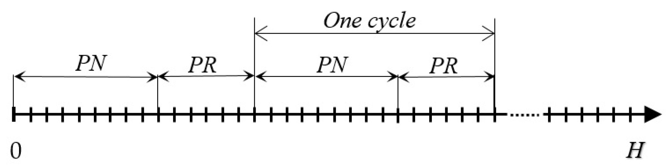
The machines M1 and M2 are subject to stochastic failures and repairs. Machine M1 manufactures new products from raw materials at a variable rate vn1(t). Machine M2 produces new and remanufactured products from returned-used ones. Indeed, M2 alternates between the production of new and remanufactured products according to a two-period plan. In the first period, which is denoted PN, the machine M2 produces new products from returned-used products of high quality at a variable rate, vn2(t). In the second period, which is denoted PR, the machine M2 produces remanufactured products from returned-used products of average quality at a variable rate, vr(t). These two periods are planned by the manufacturer. When the machine M2 switches between PN and PR, a set-up action is required. In this work, it assumed that the set-up period and cost are negligible. Thus, the machine M2 repeats a cycle that is consisted of PN and PR until the horizon will be reached (see Figure 3).
The store Sn is replenished by the machine M1 and the machine M2 when it manufactures over the period PN. The store Sr is replenished by the machine M2 when it manufactures over the period PR. The stores Sn and Sr satisfy the demands Dn(t) and Dr(t), respectively. The sold products for the primary market will be collected and returned to the manufacturer when they reach the end of their service life, θ. In the quality inspection center, the returned products will be inspected and sorted according to their quality. The returned-used products of high quality are stored in the recovery inventory Rh, and then transformed to new products by the machine M2. The returned-used products of average quality are stored in the recovery inventory Ra, and then remanufactured by the machine M2. The returned-used products of poor quality will be sold immediately to the recycler with a low price. It is supposed that the sold products for the secondary market (remanufactured products) will be destroyed when they reach the end of their service life. The number of returned-used products q(t) depends on the sales of new products in past periods. The return of used products generates the return cost cq, which includes the collecting and transporting costs of the used products.
The production of new or remanufactured products causes carbon emissions. To assess the impact of the sustainable supply chain design on the environment, this paper takes into account the carbon emissions for producing both types of products.
To simplify the writing, we define the following abbreviations:
- -
- New products from raw materials (NPFRM)
- -
- New products from used products (NPFUP)
- -
- Remanufactured products from used products (RPFUP)
Moreover, we consider the following assumptions:
- (1)
- To simplify writing and calculation, it assumed that Δt = 1.
- (2)
- It is assumed that NPFUP have same quality as for NPFRM. Thus, they are sold at the same price in the primary market.
- (3)
- Remanufactured products have lower quality than new ones. Thus, they are sold at a lower price (i.e., can > car) in the secondary market.
- (4)
- It is supposed that the machine M1 is always supplied by raw materials.
- (5)
- The demands Dn(t) and Dr(t) are distinct and stochastic.
- (6)
- When the demand either for manufactured or remanufactured products is not satisfied, it is lost with the occurrence of a lost sales cost.
- (7)
- The production cost of a NPFRM is higher than that of NPFUP (i.e., cun1 > cun2).
- (8)
- The production cost of a NPFUM is higher than that of RPFUP (i.e., cun2 > cur).
- (9)
- The lost sales cost for remanufactured products is lower than that for new ones (i.e., cbn < cbr).
- (10)
- The quantity of returned-used products q(t) depends on the new products sales in past periods.
- (11)
- As q(t) depends on the new products sales in past periods, it is supposed that the average demand for new products is higher than that for remanufactured ones.
- (12)
- The maximum production rate V1 satisfies the new products demand (i.e., V1 ≥ max (Dn(t))). This assumption ensures store Sn building.
- (13)
- The maximum production rate V2 is higher than the quantity of returned-used products, (i.e., V2 > max (q(t))). This assumption avoids having Rh or Ra always full.
- (14)
- The unit carbon emission from producing NPFRM is higher than that for NPFUM and RPFUP (i.e., en1 > en2 and en1 > er).
- (15)
- The units carbon emission from producing NPFUM and RPFUP are near each other (i.e., en2 ≈ er).
- (16)
- The unit selling price for returned products with poor quality is lower than the unit return cost of used products (i.e., cq > cp).
- (17)
- At time t = 0, there are enough products in the stores to satisfy the demands.
3. Model Formulation
It assumed that machine M1 is always replenished by raw materials. The machine M1 state is either operating or down, and it is given by:
The machine M2 state is given by:
The generation of time to repair (MTBF1 and MTBF2) and time between failures (MTTR1 and MTTR2) are exponentially distributed. When M1 is operating, the rate vn1(t) is between 0 and its maximum V1, i.e., 0 vn1(t) V1. When M1 is down, vn1(t) = 0. The machine M2 switches between the production of NPFUP and RPFUP with rates vn2(t) and vr(t), respectively, and its maximum production rate is V2.
The demands Dn(t) and Dr(t) are supplied at the beginning of each period of time, so they are satisfied from the stores at the previous period x(t − ∆t) and y(t − ∆t), respectively. Thus, when Dn(t) ≤ x(t − ∆t) and Dr(t) ≤ y(t − ∆t), the demands are totally satisfied, and then an(t) = Dn(t) and ar(t) = Dr(t). Otherwise, Dn(t) > x(t − ∆t) and Dr(t) > y(t − ∆t), a portion of the demand is satisfied, which corresponds to the store level (i.e., an(t) = x(t − ∆t) and ar(t) = y(t − ∆t)). Thus, the numbers of new and remanufactured products sold at time t are given by:
The numbers of unsatisfied demands for new and remanufactured products are determined by subtracting an(t) and ar(t) from Dn(t) and Dr(t), respectively. Thus, the numbers of unsatisfied demands for new and remanufactured products are given by the following equations:
The new and remanufactured products produced by the machines replenish the stores Sn and Sr, respectively. The stores levels x(t) and y(t)) at time t are given by:
The number of returned-used products at time t is proportional to the number of sold products at time t − ω. We denote by θ the percentage of products, relative to sales, that return from the primary market. Of course, in the case when (t − ω) < 0, there are no returns.
The returned-used products are inspected and then sorted into three categories based on their quality. The first category contains the returned-used products of high quality; the second contains the ones of average quality, and the third contains the ones of poor quality. We denote by α, β, and λ, percentages of used products of high, average, and poor qualities, respectively (with α + β + λ = 1). Thus, the number of returned products of high quality at time t is given by:
The number of returned products of average quality at time t is given by:
The number of returned products of poor quality at time t is given by:
The returned products of high quality are stored in the recovery inventory Rh that supplies the machine M2 when the period is PN. The level of the recovery inventory Rh at time t is given by:
The returned products of average quality are stored in the recovery inventory Ra that supplies the machine M2 when the period is PR. The level of the recovery inventory Ra at time t is given by:
To simplify the written equations of the production rates, we defined two variables, EN(t) and ER(t), which represent the states of M2 when it produces in PN and PR, respectively.
The stores Sn is replenished by the machines M1 and M2. The total production rate for new products is given by:
In what follows, we present the production control of both machines. Based on the machine’s states and store level, the total production rate for new products is determined. Indeed, this proposed policy controls both machines while preserving the coordination between the production of NPFUP and NPFRM, storing the products, and the return of used products.
Transforming the previous equations, we can determine the production rates of M1 and M2 separately:
The carbon emission quantity at time t equals the total of the carbon emissions from producing NPFRM, NPFUP, and RPFUP.
We determine the total profit function over the horizon [0, T] by computing the difference between the total sales revenues and the total costs.
4. Evolutionary Algorithm for Optimization
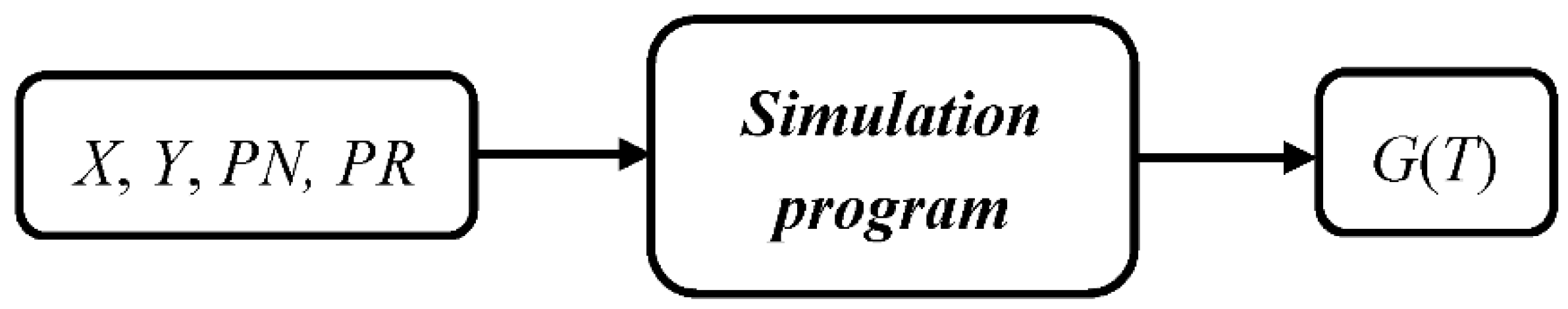
In this section, we present the proposed optimization method, which is based on an evolutionary algorithm. The general principle of the method is to gradually drive the algorithm to the optimal solution by comparing and evaluating the different solutions found by simulation. Indeed, the developed algorithm uses a simulation program, which determinates the total profit function for the values of given decision variables X, Y, PN, and PR (see Figure 4). As the total profit is determined by a stochastic function, the simulation time horizon is fixed to 107 time units. This value is chosen after a simulation experience, which allows finding a not-fluctuating value of the total profit. Furthermore, in order to obtain efficient simulation values during the optimization running, the algorithm calculates the average of 10 simulations.
The proposed evolutionary algorithm returns optimal values of decision variables (X*, Y*, PN* and PR*) that maximize the profit function. The variables PN* and PR* can vary in [1; 100,000], and for X* and Y*, it can vary in [1; 1000]. In what follows, we present a flowchart that presents the steps that the evolutionary algorithm follows.
The proposed algorithm is composed of two sub-algorithms (please see Figure 5). The first is based on an optimization method that determines one optimum by stochastically trying the values of X, Y, PN, and PR, and then compares the profit values of all of the trials. Indeed, for each try, the first sub-algorithm calls on a simulation program to determine the corresponding profit value. This value is then memorized and compared to the values of the other trials. We have chosen a suitable number of trials that is equal to 500. Indeed, as it is known in the optimization theory, the higher the trial number; the better the quality of the result. However, when the trial number is very high, the optimization method takes a long period of time. Thus, it is important to find the suitable number of trials that allows the sub-algorithm to find a good result in a reasonable amount of time. The found solution by the first sub-algorithm is considered a pseudo-optimal solution. The role of the second sub-algorithm is to improve the pseudo-optimum by testing neighborhood sets. Indeed, the second sub-algorithm stochastically tries neighbor values to that of the pseudo-optimum, and then calls on the simulation program to determine the profit values that correspond to the neighbor values. The found values are compared to the pseudo-optimum, and when a better solution is found (profit greater than the pseudo-optimum), it will be taken as a new pseudo-optimum. The second sub-algorithm repeats the trials and improves the solution by finding new pseudo-optimum and mutating the best solutions. This sub-algorithm finds the optimum after a determined trial number of neighbor values. In our study, we have fixed the trial number of neighbor values to 50 tries.
5. Results and Discussion
In this section, we conduct interesting experimental studies that are useful in practice. The proposed model is exploited to study the effect of some parameters on X*, Y*, PN*, PR*, and the environment (carbon emission). Firstly, the numerical data are introduced above. Then, we present the studies of the impact of the percentage of returned-used products and unit carbon emission cost on X*, Y*, PN* and PR*, as well as on the carbon emission.
The numerical data that we use for the simulation are presented in what follows:
- H = 107 periods
- MTBF1 = seven periods
- MTTR1 = two periods
- MTBF2 = nine periods
- MTTR2 = three periods
- V1 = 100 products/period
- V2 = 50 products/period
- ω= 1000 periods
- en1 = 25 carbon units
- en2 = seven carbon units
- er = six carbon units
- can = 90 monetary units
- car = 55 monetary units
- cun1= 25 monetary units
- cun2= 10 monetary units
- cur = eight monetary units
- cx = 0.002 monetary units
- cy = 0.001 monetary units
- cbn = 900 monetary units
- cbr = 550 monetary units
- cq = three monetary units
- cp = one monetary unit
- crh = 0.0001 monetary units
- cra = 0.0001 monetary units
- ce = one monetary unit
- α = 20%
- β = 70%
- λ = 10%
- The demand Dn(t) is generated by truncated normal distribution, in which the average = 100 and the standard deviation = 50.
- The same distribution is used for the demand Dr(t), in which the average = 25 and the standard deviation = 13.
5.1. Effect of θ on X*, Y*, PN*, PR*, and G*(T)
In this subsection, we present experiment results to show the effect of θ on X*, Y*, PN*, and PR*. The study consists of varying the value of θ (please see Table 1), and by using the evolutionary algorithm, we determine the corresponding values of X*, Y*, PN*, PR*, and G*(T). The objective of this study is to analyze the evolution of the optimal supply chain design when the quantity of returned-used products changes. Furthermore, through this study, the firm leader can perform a return strategy that maximizes the profit. By exploiting the evolutionary algorithm, we have obtained the following results:
By observing the obtained results in the table above, there are three interesting observations. The first is that the period for producing NPFUP (PN) increases when the quantity of returned-used products increases. As the NPFUP consists of new products produced from returned-used ones, it is more beneficial for producing NPFUP than producing new products from raw materials (NPFRM). Indeed, when the quantity of returned-used products increases, the number of returned products of high quality increases (wh(t)); then, to take advantage, it shall increase the production of NPFUP to increase the profit. However, in our case, when θ exceeds 40%, the profit starts to decrease, despite the increasing of NPFUP. Indeed, the optimal value of the profit G*(T) has a maximum, which is our second observation. To explain this aspect, we need to observe the number of returned products of average quality (wa(t)). In our case, we have the percentage of returned products of average quality β = 70%, and when θ = 40%, that means that = (see Equation (11)), in which is the number of new products sold in the previous periods. Also, when θ = 40%, we have = . Thus, when θ = 40%, the demand for new products are well satisfied as the NPFUP enhances the level of the new products’ store. Consequently, increases and can be near to the value of the new product demand. Thus, the , as the average of the remanufactured products demand (Dr(t)) is equal to 25. Thus, this demand is mostly satisfied. Consequently, when θ exceeds 40%, the remanufactured products demand is more satisfied. However, as the proposed production politic limits the production in order to respect the store capacity, the returned products of average quality, which are counted within the recovery inventory Ra, are accumulating, in which case the inventory cost becomes very important. Consequently, the total profit decreases, even as NPFUP increases. In addition, when θ is less than 40%, we have observed that the period PR* is higher than PN*. In this case, the demand for remanufactured products is poorly satisfied, but for the new ones, the demand is almost satisfied, as the system can provide NPFRM when NPFUP is low. As the lost sale costs are high, thus, the optimal strategy is to favor the production of RPFUP over the production of NPFUP. The third observation is that when θ exceeds 40%, the optimal period PR* becomes almost constant. Indeed, as in this case, when the remanufactured products demand is satisfied, the production of NPFUP should be almost constant to avoid the increasing storage of remanufactured products. In conclusion, this study is useful for a firm leader that has the option to manage the return of used products. Indeed, in practice, the used products, such as the car turbochargers, are collected according to the firm needs. Thus, this study is useful for finding the optimal design of a manufacturing/remanufacturing firm while considering the storage, production politic, and return of used products.
5.2. Impact of Returned-Used Products Quality on X*, Y*, PN*, PR*, and G*(T)
In this subsection, we present experiment results to show the effect of returned-used products quality on X*, Y*, PN*, PR*, and G*(T). The study consists of varying the values of α, β, and λ, and by using the evolutionary algorithm, we determine the corresponding values of X*, Y*, PN*, PR*, and G*(T). The objective of this study is to find the optimal design when the quality of the returned-used products changes. We use the same data that was used in the previous subsection, and the value of θ is fixed to 40%. In addition, to focus on the quality study, we have fixed the value of the lost sales cbn and cbr to 90 and 55 monetary units, respectively. By exploiting the evolutionary algorithm, we have obtained the following results.
By observing the obtained results in Table 2, the first observation is that when the number of returned products of high quality increases, the profit increases. Of course, when the number of returned products of high quality increases, the producer increases the production of NPFUP and decreases the production of NPFRM, as the cost for producing one NPFUP is cheaper than for NPFRM. Indeed, the carbon emissions from producing NPFRM are more important than for NPFUP, as it makes the production of NPFRM more expensive. Thus, in order to take advantage of the increasing of the returned products of high quality, it is obvious to produce NPFUP rather than NPFRM. Consequently, as the machine switches between PN and PR, the period PN increases, but PR decreases. Indeed, in this, the producer should favor the production of NPFUP over RPFUP. The values of the optimal capacity are related to the production periods. In general, when PN or PR increases, X* or Y* increases. In lines 6 and 7 of Table 2, we have increased the number of returned products of poor quality while keeping the same proportionality for returned products of high and average qualities. As observed, when the number of returned products of poor quality increases, the total profit decreases. Indeed, the returned products of poor quality are losses for the firm, as they cannot be used for producing either new or remanufactured products. Furthermore, the producer is obliged to sell them to a tertiary market at a lower price than its purchase price. In conclusion, this study shows that the higher the quality of the returned-used products, the more the manufacturing/remanufacturing firm increases its profits. In practice, the firm leader needs to find an optimal arrangement with the collector that can provide returned-used products of good quality, but at a higher price. Thus, according to the customer demand, the firm leader shall find a compromise between the quality and the price of the returned-used products. In the next study, we are interested in studying the impact of the quality of the returned-used products on the environment.
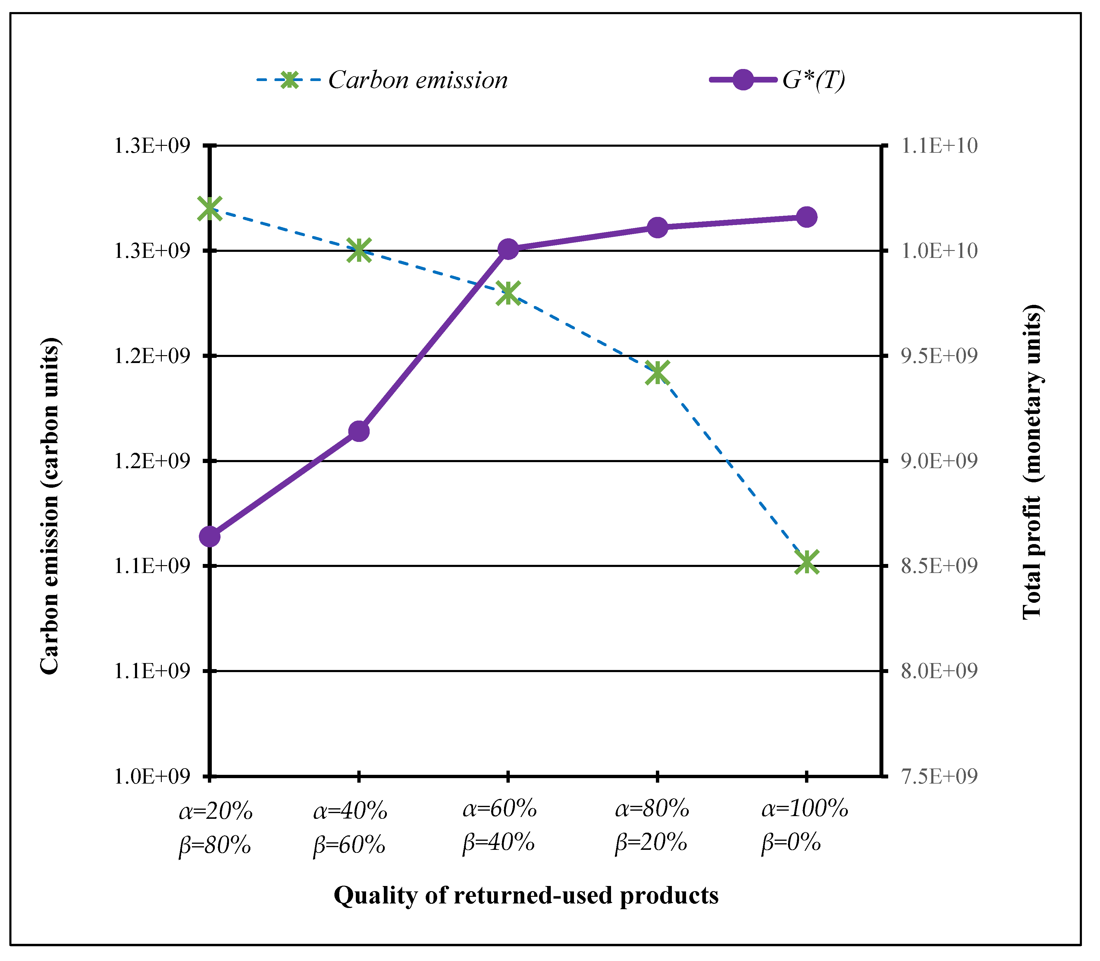
5.3. Impact of Returned-Used Products Quality on Carbon Emission and G*(T)
In this subsection, we present experiment results to show the effect of the quality of the returned-used products on carbon emissions and the optimal profit. As it was found in the previous subsection that the returned products of poor quality are useless for the firm, in this study, we have an interest in focusing on the impact of returned products of high and average quality. Thus, we consider that the number of returned products of poor quality is equal to zero. This study consists of varying the value of α and β, and by using the evolutionary algorithm, we determine the corresponding values for carbon emissions (Equation (22)) and G*(T). We use the same data that was used in the previous subsection, and the value of λ is fixed to 0%. Based on carbon emissions regulations, this study helps the firm leader make a decision on the return rate according to the quality of the used products. The result are presented in the following figure.
By observing the obtained results in Figure 6 the first observation is that when the number of returned products of high quality increases, the carbon emission decreases, and the optimal total profit increases. Indeed, when the number of returned products of high quality increases, the producer increases the production of NPFUP and decreases the production of NPFRM. Since the carbon emissions from producing NPFRM are more important than for NPFUP, it makes the total carbon emission low, and at the same time decreases the emission cost. Furthermore, as the cost for producing one NPFUP is cheaper than for NPFRM, the total profit of course increases. The second observation is that the increase in the total profit becomes low when α exceeds 60% (i.e., β < 60%). Indeed, when the number of returned products of average quality decreases, the demand for remanufactured products is poorly satisfied, and the lost sales costs increase, which has an impact on the increasing of the total profit. Thus, for the case in which the lost sales costs are high, the profit may decrease (i.e., the curve of the total profit may reverse). In conclusion, the production of NPFUP or of RPFUP has the same impact on the environment. However, the production of NPFUP has a greater potential impact on the environment, because the NPFUP products are considered as new one, and since the production of NPFRM emits a high quantity of carbon compared to NPFUP, the production of NPFRM potentially decreases carbon emissions. Therefore, as the proposed manufacturing/remanufacturing system has two demands for new and remanufactured products, the producer should increase the return of used products in order to increase the production of NPFUP and satisfy the demand of RPFUP. Furthermore, the production of RPFUP may have a potential impact on the environment if the customers prefer buying remanufactured products instead of new ones. Therefore, we have an interest in studying the carbon emissions emitted by each type of returned-used product, which is what we will study in the next subsection.
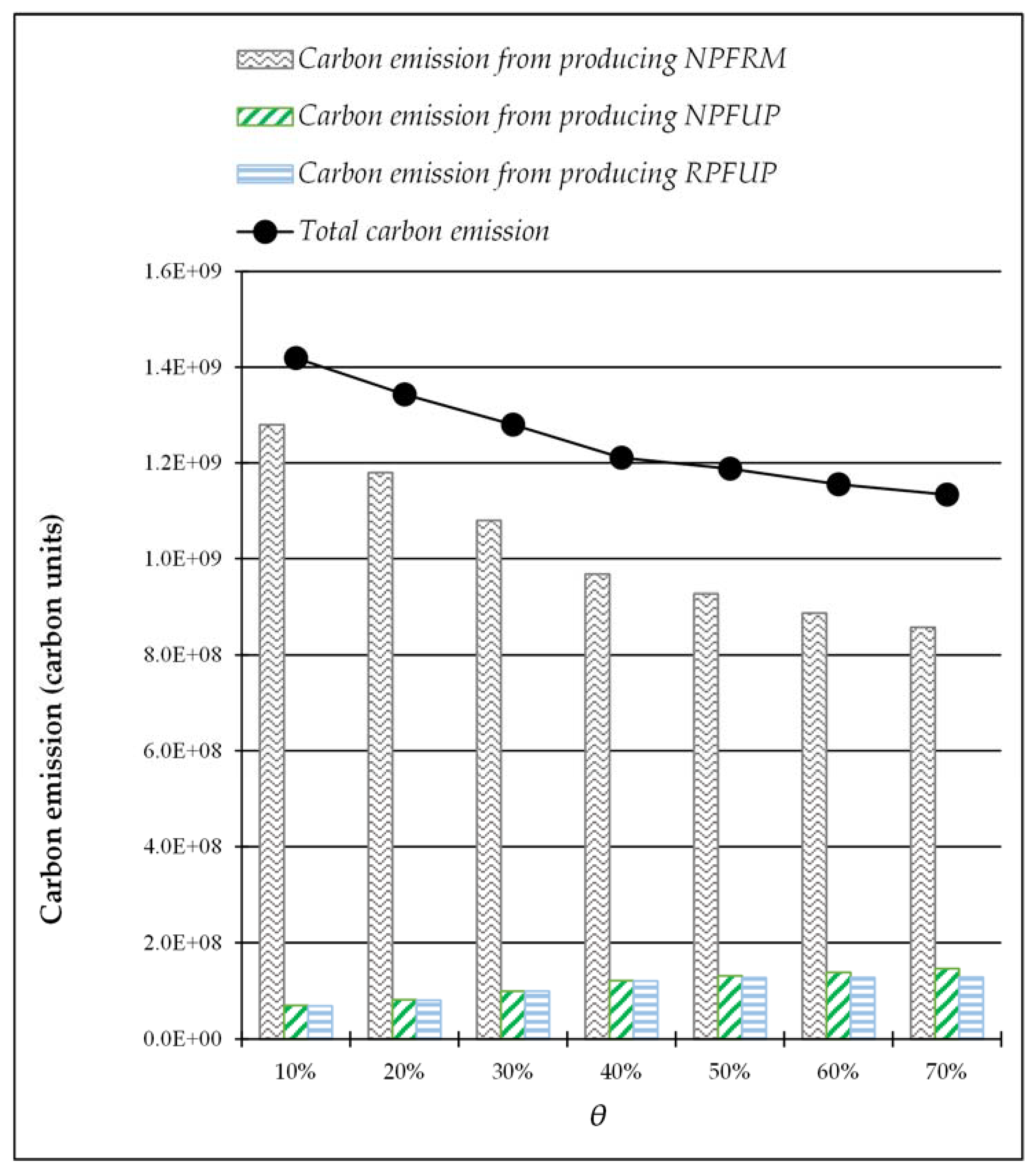
5.4. Impact of Returned-Used Products Quantity on Carbon Emission
In this subsection, we present experimental results to show the effect of the quantity of returned-used products on the carbon emissions. The objective is to study the reparation of the carbon emissions from producing each type of product (NPFRM, NPFUP, and RPFUP). As in the previous subsection, we consider that the number of returned products of poor quality is equal to zero. In this subsection, we vary the value of θ, and we determine the corresponding values of carbon emissions for each type of product. We use the same data that was used in the previous subsection, both values of α and β are fixed to 50%, and for the carbon emissions, en2 = er = 6 carbon units. The results are presented in the following figure.
By observing the obtained results in Figure 7, the first observation is that when the quantity of returned-used products increases, the total carbon emissions decrease. This observation is already explained in the previous subsection. Indeed, when the quantity of returned-used products increases, the number of returned products of high quality increase, and then the number of NPFRM decreases and the number of NPFUP increases. Thus, the carbon emissions decrease, since the carbon emissions from producing NPFRM is very high compared to that for NPFUP. The second observation is that the carbon emissions from producing NPFUP increase when the returned-used products quantity increases, which is obvious, as the producer increases the production of NPFUP to maximize the total profit. Also, the carbon emissions from producing RPFUP increase. However, when θ exceeds 40%, the emissions seem to be constant. As we have explained in Section 5.1, the production of RPFUP becomes constant when θ exceeds 40%. This is due to the production politic that limits the production according to the store capacity and the demand of remanufactured products.
In conclusion, the return of used products decreases the carbon emissions. To increase the total profit and decrease the carbon emissions, the firm leader needs to attract more customers to buy remanufactured products instead of new ones, at a low price compared to new ones. Furthermore, in practice, the firm leader needs to explore the possibility of finding an arrangement with the collector in order to receive used products of high quality. This is dependent on the price of the collected used products.
6. Conclusions
This work proposes a new design for a manufacturing/remanufacturing system that distinguishes new and remanufacturing products, and considers the quality of returned-used products. The proposed manufacturing/remanufacturing system is composed of two parallel machines. The first machine produces new products from raw materials, and the second one alternates the production of new products from used ones of high quality with remanufactured products from used ones of average quality. The new and remanufactured products are destined for the primary and secondary market, respectively. The used products of poor quality are sold to the tertiary market at a low price. To make the proposed system more realistic, it assumed that both machines are subject to random repairs and failures, the demands for new products and remanufactured ones are stochastic, the quantity of returned-used products is proportional to the sales in the previous periods. Furthermore, the returned-used products are sorted in three quality levels, and carbon emissions are also considered. A model that is based on discrete modeling is developed to describe the system and consider the above issues. An optimization method based on an evolutionary algorithm is developed to find the optimal values of the store’s capacities and the ideal remanufacturing periods of new and remanufactured products. Finally, the developed model and the optimization method are exploited to obtain numerical results within different case studies. The results show the impact of the quantity and quality of the returned-used products on the optimal values for store capacities and the remanufacturing periods of new and remanufactured products. In addition, the optimal total profit, the total carbon emissions, and the emissions emitted by each type of product are determined according to the quantity and quality of the returned-used products.
This work is not exempt from limitations. First, the machines’ maintenance costs are not considered. However, they usually have an impact on the total profit. Second, the quality levels of the returned-used products are supposed to be constant. However, in practice, the quality levels are random.
In future research, we will consider the quantity and quality of returned-used products to be stochastic. Furthermore, we will assume a multi-level quality of used products. In addition, we will consider the machine degradation according to the quality level of the used products. We will also consider transport vehicles between stores and markets when considering carbon emissions.
Author Contributions
S.T. is the responsible for conducting this research. S.T. proposed the main paper contribution and developed the mathematical model and the optimization method. N.R. supervised this work and contributed to revise this paper.
Funding
This research received no external funding.
Conflicts of Interest
The authors declare no conflict of interest.
References
- Turki, S.; Rezg, N. Optimization of manufacturing supply chain with stochastic demand and planned delivery time. J. Traffic Transp. Eng. 2017, 5, 32–43. [Google Scholar]
- Son, D.; Kim, S.; Park, H.; Jeong, B. Closed-Loop Supply Chain Planning Model of Rare Metals. Sustainability 2018, 10, 1061. [Google Scholar] [CrossRef]
- Liu, C.; Yang, J.; Lian, J.; Li, W.; Evans, S.; Yin, Y. Sustainable performance oriented operational decision-making of single machine systems with deterministic product arrival time. J. Clean. Prod. 2014, 85, 318–330. [Google Scholar] [CrossRef]
- Kim, H.; Lee, C.W. The Effects of Customer Perception and Participation in Sustainable Supply Chain Management: A Smartphone Industry Study. Sustainability 2018, 10, 2271. [Google Scholar] [CrossRef]
- Turki, S.; Bistorin, O.; Rezg, N. Infinitesimal perturbation analysis based optimization for a manufacturing-remanufacturing system. In Proceedings of the 2013 IEEE 18th Conference on Emerging Technologies & Factory Automation (ETFA), Cagliari, Italy, 10–13 September 2013; pp. 1–8. [Google Scholar] [CrossRef]
- Huang, M.; Yi, P.; Shi, T. Triple recycling channel strategies for remanufacturing of construction machinery in a retailer-dominated closed-loop supply chain. Sustainability 2017, 9, 2167. [Google Scholar] [CrossRef]
- Turki, S.; Rezg, N. Unreliable manufacturing supply chain optimisation based on an infinitesimal perturbation analysis. Int. J. Syst. Sci. Oper. Logist. 2016. [Google Scholar] [CrossRef]
- Turki, S.; Didukh, S.; Sauvey, C.; Rezg, N. Optimization and Analysis of a Manufacturing–Remanufacturing–Transport–Warehousing System within a Closed-Loop Supply Chain. Sustainability 2017, 9, 561. [Google Scholar] [CrossRef]
- Xu, Z.; Pokharel, S.; Elomri, A.; Mutlu, F. Emission policies and their analysis for the design of hybrid and dedicated closed-loop supply chains. J. Clean. Prod. 2017, 142, 4152–4168. [Google Scholar] [CrossRef]
- Klumpp, M. How to Achieve Supply Chain Sustainability Efficiently? Taming the Triple Bottom Line Split Business Cycle. Sustainability 2018, 10, 397. [Google Scholar] [CrossRef]
- Fulton, L.; Mejia, A.; Arioli, M.; Dematera, K.; Lah, O. Climate change mitigation pathways for Southeast Asia: CO2 emissions reduction policies for the energy and transport sectors. Sustainability 2017, 9, 1160. [Google Scholar] [CrossRef]
- Centobelli, P.; Cerchione, R.; Esposito, E. Environmental sustainability in the service industry of transportation and logistics service providers: Systematic literature review and research directions. Transp. Res. Part D Transp. Environ. 2017, 53, 454–470. [Google Scholar] [CrossRef]
- Centobelli, P.; Cerchione, R.; Esposito, E. Environmental sustainability and energy-efficient supply chain management: A review of research trends and proposed guidelines. Energies 2018, 11, 275. [Google Scholar] [CrossRef]
- Turki, S.; Sauvey, C.; Rezg, N. Modelling and optimization of a manufacturing/remanufacturing system with storage facility under carbon cap and trade policy. J. Clean. Prod. 2018, 193, 441–458. [Google Scholar] [CrossRef]
- Zhang, L.; Yang, W.; Yuan, Y.; Zhou, R. An integrated carbon policy-based interactive strategy for carbon reduction and economic development in a construction material supply chain. Sustainability 2107, 9, 2107. [Google Scholar] [CrossRef]
- Wang, J.; Huang, X. The Optimal Carbon Reduction and Return Strategies under Carbon Tax Policy. Sustainability 2018, 10, 2471. [Google Scholar] [CrossRef]
- Jin, M.; Shi, X.; Emrouznejad, A.; Yang, F. Determining the optimal carbon tax rate based on data envelopment analysis. J. Clean. Prod. 2018, 172, 900–908. [Google Scholar] [CrossRef]
- Yuan, B.; Gu, B.; Guo, J.; Xia, L.; Xu, C. The optimal decisions for a sustainable supply chain with carbon information asymmetry under cap-and-trade. Sustainability 2018, 10, 1002. [Google Scholar] [CrossRef]
- Chang, X.; Li, Y.; Zhao, Y.; Liu, W.; Wu, J. Effects of carbon permits allocation methods on remanufacturing production decisions. J. Clean. Prod. 2017, 152, 281–294. [Google Scholar] [CrossRef]
- Cai, X.; Lai, M.; Li, X.; Li, Y.; Wu, X. Optimal acquisition and production policy in a hybrid manufacturing/remanufacturing system with core acquisition at different quality levels. Eur. J. Oper. Res. 2014, 233, 374–382. [Google Scholar] [CrossRef]
- Shu, T.; Xu, J.; Chen, S.; Wang, S.; Lai, K.K. Remanufacturing Decisions with WTP Discrepancy and Uncertain Quality of Product Returns. Sustainability 2018, 10, 2123. [Google Scholar] [CrossRef]
- Zhang, Z.; Zhang, Q.; Liu, Z.; Zheng, X. Static and Dynamic Pricing Strategies in a Closed-Loop Supply Chain with Reference Quality Effects. Sustainability 2018, 10, 157. [Google Scholar] [CrossRef]
- Moshtagh, M.S.; Taleizadeh, A.A. Stochastic integrated manufacturing and remanufacturing model with shortage, rework and quality based return rate in a closed loop supply chain. J. Clean. Prod. 2017, 141, 1548–1573. [Google Scholar] [CrossRef]
- Turki, S.; Bistorin, O.; Rezg, N. Optimization of stochastic fluid model using perturbation analysis: A manufacturingremanufacturing system with stochastic demand and stochastic returned products. In Proceedings of the 2014 IEEE 11th International Conference on Networking, Sensing and Control (ICNSC), Miami, FL, USA, 7–9 April 2014; pp. 1–6. [Google Scholar]
- Song, B.D.; Ko, Y.D. Effect of inspection policies and residual value of collected used products: A mathematical model and genetic algorithm for a closed-loop green manufacturing system. Sustainability 2017, 9, 1589. [Google Scholar] [CrossRef]
- Turki, S.; Hennequin, S.; Sauer, N. Performance evaluation of a failure-prone manufacturing system with time to delivery and stochastic demand. IFAC Proc. Vol. 2009, 42, 516–521. [Google Scholar]
- Turki, S.; Hennequin, S.; Sauer, N. Perturbation analysis for continuous and discrete flow models: A study of the delivery time impact on the optimal buffer level. Int. J. Prod. Res. 2013, 51, 4011–4044. [Google Scholar] [CrossRef]
- Turki, S.; Hennequin, S.; Sauer, N. Perturbation analysis-based optimisation for a failure-prone manufacturing system with constant delivery time and stochastic demand. Int. J. Adv. Oper. Manag. 2012, 4, 124–153. [Google Scholar] [CrossRef]
- Turki, S.; Bistorin, O.; Rezg, N. Infinitesimal perturbation analysis based optimization for a manufacturing system with delivery time. In Proceedings of the 2012 IEEE 17th Conference on Emerging Technologies & Factory Automation (ETFA), Krakow, Poland, 17–21 September 2012; pp. 1–8. [Google Scholar]
- Trabelsi, W.; Sauvey, C.; Sauer, N. Heuristics and metaheuristics for mixed blocking constraints flowshop scheduling problems. Comput. Oper. Res. 2012, 39, 2520–2527. [Google Scholar] [CrossRef]
Figure 1.
Time horizon discretization.
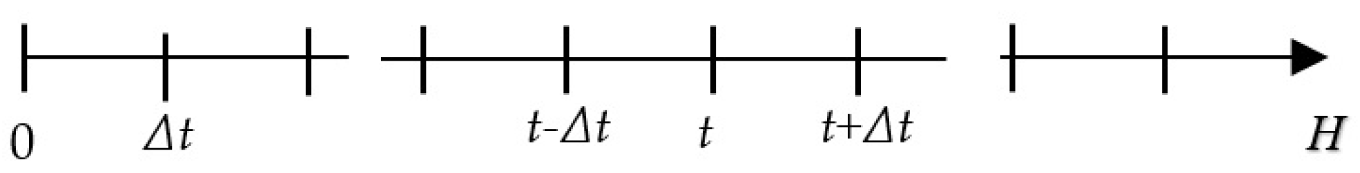
Figure 2.
Manufacturing/remanufacturing system.
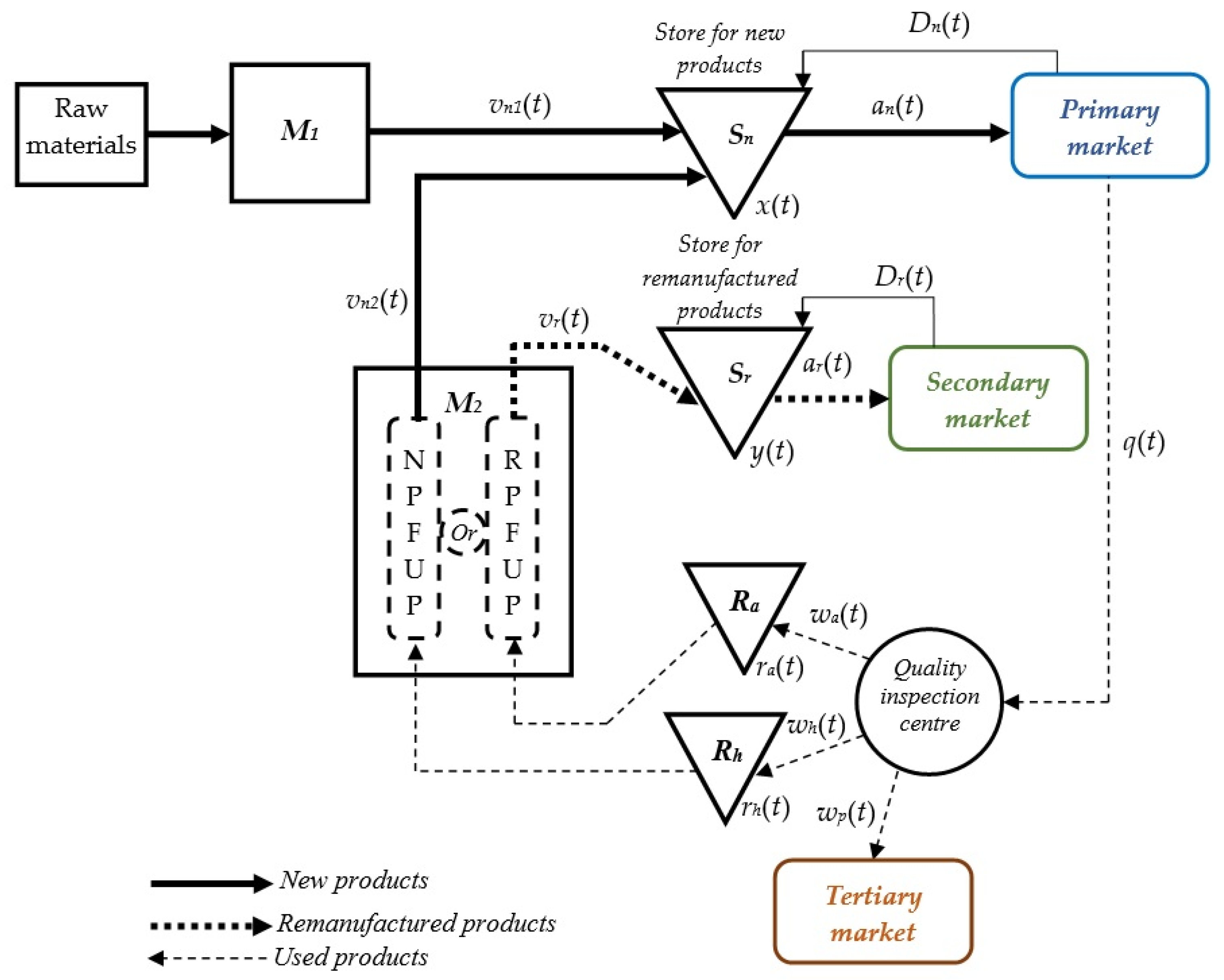
Figure 3.
First (PN) and second (PR) periods.

Figure 4.
Simulation program.

Figure 5.
Evolutionary algorithm.
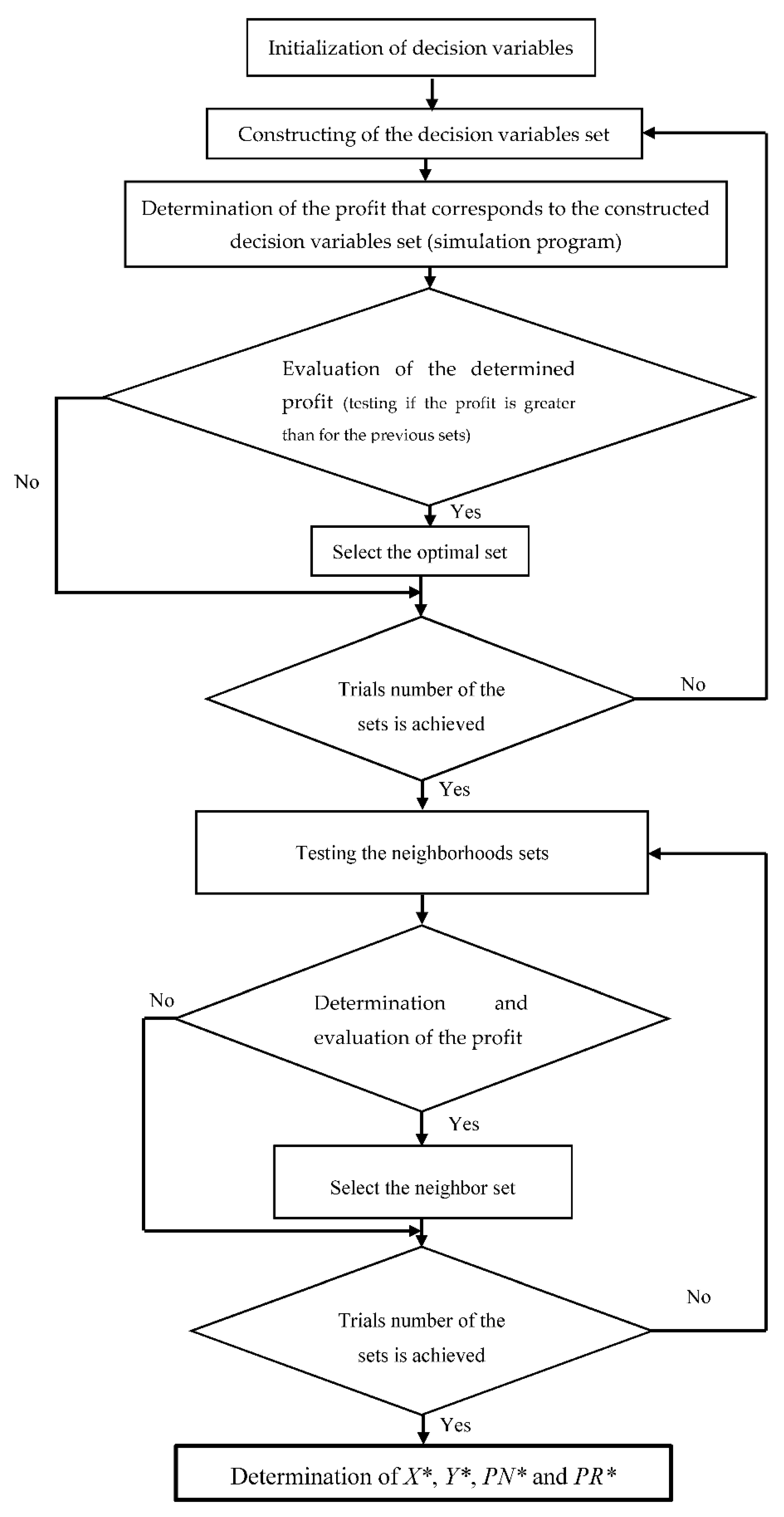
Figure 6.
Impact of returned-used products quality on carbon emission and G*(T).

Figure 7.
Reparation of the carbon emissions according to product type.


Table 1.
Effect of returned-used products on X*, Y*, PN*, PR*, and G*(T).
| θ | PN* | PR* | X* | Y* | G*(T) |
|---|---|---|---|---|---|
| 10% | 282 | 1804 | 107 | 13 | 4.83510 × 10⁹ |
| 20% | 334 | 1681 | 135 | 19 | 5.32092 × 10⁹ |
| 30% | 407 | 1473 | 163 | 24 | 5.80944 × 10⁹ |
| 40% | 682 | 1249 | 186 | 49 | 6.12112 × 10⁹ |
| 50% | 809 | 1262 | 189 | 52 | 5.99288 × 10⁹ |
| 60% | 1083 | 1266 | 192 | 58 | 5.84654 × 10⁹ |
Table 2.
Impact of returned-used products quality on X*, Y*, PN*, PR*, and G*(T).
| α | β | λ | PN* | PR* | X* | Y* | G*(T) |
|---|---|---|---|---|---|---|---|
| 10% | 80% | 10% | 544 | 1301 | 153 | 63 | 7.43982 × 10⁹ |
| 20% | 70% | 10% | 683 | 1164 | 168 | 59 | 7.88543 × 10⁹ |
| 30% | 60% | 10% | 802 | 1011 | 179 | 54 | 8.64020 × 10⁹ |
| 40% | 50% | 10% | 961 | 903 | 183 | 49 | 9.30825 × 10⁹ |
| 50% | 40% | 10% | 1092 | 812 | 183 | 43 | 9.89530 × 10⁹ |
| 40% | 40% | 20% | 898 | 872 | 180 | 50 | 9.13204 × 10⁹ |
| 35% | 35% | 30% | 861 | 848 | 178 | 51 | 8.99081 × 10⁹ |
© 2018 by the authors. Licensee MDPI, Basel, Switzerland. This article is an open access article distributed under the terms and conditions of the Creative Commons Attribution (CC BY) license (http://creativecommons.org/licenses/by/4.0/).
Share and Cite
MDPI and ACS Style
Turki, S.; Rezg, N. Impact of the Quality of Returned-Used Products on the Optimal Design of a Manufacturing/Remanufacturing System under Carbon Emissions Constraints. Sustainability 2018, 10, 3197. https://doi.org/10.3390/su10093197
AMA Style
Turki S, Rezg N. Impact of the Quality of Returned-Used Products on the Optimal Design of a Manufacturing/Remanufacturing System under Carbon Emissions Constraints. Sustainability. 2018; 10(9):3197. https://doi.org/10.3390/su10093197
Chicago/Turabian StyleTurki, Sadok, and Nidhal Rezg. 2018. "Impact of the Quality of Returned-Used Products on the Optimal Design of a Manufacturing/Remanufacturing System under Carbon Emissions Constraints" Sustainability 10, no. 9: 3197. https://doi.org/10.3390/su10093197
Note that from the first issue of 2016, this journal uses article numbers instead of page numbers. See further details here.