Re-Planning the Intermodal Transportation of Emergency Medical Supplies with Updated Transfer Centers


1
College of Economics and Management, Northwest A & F University, Yangling 712100, China
2
Department of Industrial and Systems Engineering, The Hong Kong Polytechnic University, Hung Hom, Hong Kong, China
3
School of Management Engineering and Business, Hebei University of Engineering, Handan 056038, China
*
Author to whom correspondence should be addressed.
Sustainability 2018, 10(8), 2827; https://doi.org/10.3390/su10082827
Submission received: 30 June 2018
/
Revised: 30 July 2018
/
Accepted: 30 July 2018
/
Published: 9 August 2018
(This article belongs to the Section Sustainable Transportation)
Abstract
:Helicopters and vehicles are often jointly used to transport key relief supplies and respond to disaster situations when supply nodes are far away from demand nodes or the key roads to affected areas are cut off. Emergency transfer centers (ETCs) are often changed due to secondary disasters and further rescue, so the extant intermodal transportation plan of helicopters and vehicles needs to be adjusted accordingly. Disruption management is used to re-plan emergency intermodal transportation with updated ETCs in this study. The basic idea of disruption management is to minimize the negative impact resulting from unexpected events. To measure the impact of updated ETCs on the extant plan, the authors consider three kinds of rescue participators, that is, supply recipients, rescue drivers, and transport schedulers, whose main concerns are supply arrival time, intermodal routes and transportation capacity, respectively. Based on the measurement, the authors develop a recovery model for minimizing the disturbance caused by the updated ETCs and design an improved genetic algorithm to generate solutions for the recovery model. Numerical experiments verify the effectiveness of this model and algorithm and discern that this disruption management method could produce recovery plans with shorter average waiting times, smaller disturbances for all the supply arrival times, intermodal routes and transportation capacity, and shorter running times. The comparison shows the advantage of this disruption management method over the rescheduling method.
1. Introduction
To respond to large-scale disasters, the transportation of relief supplies is important but has many kinds of challenges, particularly for key resources such as medical supplies [1,2,3,4]. Since victims have pressing and urgent demands, the timely delivery of medical supplies plays an important role in reducing loss of life caused by disasters [5,6]. Many studies have contributed to the location and distribution of emergency medical services and supplies, such as the medical service location [6,7,8,9] and medical supply distribution [5,10,11]. Differing from these extant studies, the current authors are concerned with the emergency intermodal transportation of medical supplies using helicopters and vehicles (ambulance and other road transportation are called “vehicles”, for convenience, which are used to transport medical supplies by road in response to disasters).
Erdemir et al. [12] stated that the advantages of each transportation mode depend on specific factors such as the distance, disaster types and locations. When the number of helicopters is limited in response to large-scale disasters or the key roads to mountain towns are cut off, the joint transportation of helicopters and vehicles is often conducted. During the 2008 Sichuan earthquake and the 2013 Shantou flood, some key roads to affected areas were cut off, and in 2010, the Yushu earthquake affected towns that were far away from supply points, so helicopters were used jointly with vehicles.
To deal with this kind of specific emergency situation, Ruan et al. [13,14] developed clustering-based optimization models to generate the location of transfer points and intermodal transportation routes. The authors continue to focus on this kind of specific situation, as shown in Figure 1: The inbound relief supplies are collected at the large collecting and distributing hub (LCDH), then transported to emergency transfer centers (ETCs) by helicopters, and finally delivered to medical aid points (MAPs) by vehicles. The authors assume that the disaster command center can coordinate all the rescue resources used in the intermodal transportation, such as helicopters and vehicles.
The decision objective of the authors’ previous work [13,14] was to produce intermodal transportation plans, that is, to determine the locations of ETCs and the intermodal routes from the LCDH to ETCs and then to MAPs. However, in the iterative implementation of intermodal transportation plans, there are often some changes that occur in the intermodal network, such as the adding or cancelling of transportation nodes. LCDH, which is usually set up at the airport closest to the affected areas, has a low probability for change due to huge assembly costs and long construction time. The change of a specific MAP often has subtle effects on intermodal routes, especially for helicopters. Conversely, a change of ETCs often occurs with the development of secondary disasters and rescue works, and the cancelling or adding of a specific ETC might have a larger impact on both helicopter and vehicle routes, as Figure 1 shows. Motivated by this observation, the authors are concerned with how to re-plan intermodal transportation when some ETCs are cancelled or added.
To deal with the above problem, the authors use the disruption management idea to formulate recovery plans for intermodal transportation with updated ETCs. To summarize, the contributions of the work include:
- A disruption measurement method to quantify the effects of updated ETCs on intermodal transportation from three aspects: Supply arrival time, intermodal routes and transportation capacity. Supply arrival time involves the receiving arrangement at ETCs and MAPs, and probably has impact on both the efficiency of intermodal transportation and the utility of medical supplies. Intermodal routes impact the delivery plan and driving behavior because drivers traveling more familiar routes often take less time and make more smooth transitions. Transportation capacity impacts the service efficiency of helicopters and vehicles, since different helicopter and vehicle capacities may serve different numbers of ETCs and MAPs.
- Based on disruption measurement, the authors formulate a recovery model of intermodal transportation, aiming at minimizing the effects of updated ETCs on the original intermodal plan. The optimization model is built according to the disruption management idea, that is, to minimize the negative impact of unexpected events on the original plans. Since supply arrival time, intermodal routes and transportation capacity in the disruption measurement are considered, this recovery model is constructed to obtain adjusted transportation routes with higher efficiency and utility.
- A genetic algorithm (GA)-based solving algorithm of the recovery model is designed. Using the algorithm, a multilevel encoding method and simplification strategies are applied. The multilevel encoding method can clearly represent each intermodal route with only three real numbers. The simplification strategies are also designed based on the disruption management idea, aiming at reducing the solution space to the best extent possible. Considering the encoding method and simplification strategies, the algorithm is designed to take as little time as possible to timely produce adjusted intermodal transportation plans in response to disasters.
The rest of the paper is organized as follows. A literature review on related works is presented in the following section. Section 3 presents a disruption measurement method of the intermodal transportation with updated ETCs. Section 4 discusses the formulation of the recovery model based on the disruption measurement. Section 5 presents the improved GA-based solving algorithm. Section 6 examines the experiments conducted to verify the effectiveness and advantage of the work. Section 7 concludes the work with discussions on the limitations and future directions.
2. Literature Review
2.1. Helicopter Transportation in Disaster Rescue
When it is difficult or impossible to timely reach affected areas by land due to damaged roads or long distances between supply and demand nodes, helicopters are often used to transport key relief resources such as medical supplies and personnel [15,16]. Some studies on helicopter emergency operations have been reported.
Barbarosoğlu et al. [17] developed a helicopter planning model in response to disasters, consisting of two steps: The aim of tactical decisions in the first step is to determine the helicopter fleet, pilot assignments to helicopters and the total number of tours, and the aim of operational decisions in the second step is to determine helicopter routes among the operation base and disaster points. Özdamar [18] further contributed a helicopter planning system including a mathematical model and a Route Management Procedure (RMP), aiming at minimizing the total mission time in response to disasters. Erdemir et al. [12] presented two location-coverage models for simultaneously locating ground ambulances, air ambulances and transfer points, which could deal with the situation when the remote incident scenarios do not have suitable areas nearby for helicopters to safely land. Matsumoto et al. [16] observed that one difficulty encountered by doctor-helicopter rescue systems is the operation of the doctor-helicopter fleet during relief activities.
These studies have observed the advantages of helicopter transportation in specific emergency situations, presenting some effective solutions for helicopter emergency planning. However, these models did not consider the joint transportation of multiple transportation modes.
2.2. Techniques on Dealing with Disturbed Transportation
Taken from the literature, two kinds of techniques can be used to deal with such disturbed transportation, that is, the rescheduling method [19,20,21] and the disruption management method [22,23,24]. The rescheduling method aims at reoptimizing the whole system subject to the status when unexpected events occur, so it might produce optimal solutions under specific objectives. However, the solutions probably bring about a large disturbance to make the recovered plans infeasible [23,24]. Disruption management is a kind of emerging idea for dealing with unexpected events, which has been widely used in various areas such as supply chain management [25,26,27,28,29] and machine job scheduling [30,31,32]. These studies have observed the advantages of disruption management in dealing with unexpected events.
The authors of this study try to use the disruption management idea to deal with the updated ETCs in the intermodal transportation of helicopters and vehicles. To the best of the authors’ knowledge, few studies are reported in the literature to apply the disruption management idea to the recovery of intermodal transportation systems. This study provides a different method to re-plan the disturbed intermodal transportation.
3. Disruption Measurement of Updated Emergency Transfer Centers (ETCs)
Disruption measurement refers to quantifying the effects caused by unexpected events, which is the basis of disruption management. During iterative implementations of the intermodal plan of helicopters and vehicles, both adding and cancelling emergency transfer centers (ETCs) will reshape the intermodal transportation network and, consequently, bring about disturbances to the original intermodal plan. Thus, to model the recovery problem of intermodal transportation with updated ETCs, one should first measure the effects caused by updated ETCs.
Since different participants such as supply recipients, rescue drivers, and transport schedulers are involved in emergency intermodal transportation, the disruption measurement should reflect the respective concerns of the related participants. The authors of this work consider the measurement from three aspects: supply arrival time, intermodal routes and transportation capacity, to reflect the receiving arrangement at ETCs and medical aid points (MAPs), the delivery plan and driving behavior, and the service efficiency of helicopters and vehicles, respectively.
3.1. Measurement on Supply Arrival Time
The supply arrival time at emergency transfer centers (ETCs) and medical aid points (MAPs) impacts the receiving arrangement, such as for transfer staff and tools. Thus, it is necessary to consider the changes to supply arrival times when re-planning intermodal transportation.
Let and , respectively, denote the number of ETCs and MAPs in the original intermodal plan, denote the planned supply arrival time of MAP covered by ETC , and denote the recovered arrival time of MAP , , . According to the practical operations, the disturbance of supply arrival time of MAP could be measured by:
where is a symbol variable and denotes time deviation parameter: if , , if , , and if , . The disturbance measurement for all the MAPs on supply arrival time is:
where denotes the unit penalty coefficient of time disturbance and denotes the set of MAPs covered by ETC in the original plan. (Although the number of ETCs and the covered MAPs by each ETC are probably changed, the MAPs are not changed, so the MAPs in the original plan are used as the reference.)
3.2. Measurement on Intermodal Routes
Regarding helicopter and vehicle drivers, disturbance on intermodal routes should be minimized mainly due to the following three reasons. First, in response to disasters, scarce helicopters and vehicles are often in full use, that is, they will be assigned with new delivery tasks when finishing current ones. Second, it often takes less time for drivers delivering equivalent tasks on more familiar routes because most drivers need more time to know new roads and make contact with new medical aid points (MAPs). Third, adjustments of intermodal routes probably cause changes to the loading and flying plans of corresponding helicopters, the transfer plans at emergency transfer centers (ETCs), the delivery plans of corresponding vehicles, and the receiving plans at MAPs.
Here, the disruption measurement of the helicopter flight routes is analyzed. Let and respectively denote the set of ETCs in the original and recovered plans, then the set of original helicopter flight routes can be expressed by , where denotes the large collecting and distributing hub (LCDH) and denotes the number of available helicopters at the LCDH; The set of recovered helicopter flight routes is . The disturbance of helicopter flight routes could then be measured by:
where denotes the unit penalty coefficient of helicopter route disturbance. is the deviation parameter of helicopter routes: When the original helicopter flight route belongs to , , otherwise ; when the recovered helicopter flight route belongs to , , otherwise .
Meanwhile, the updated ETCs might result in a change of vehicle delivery routes in the original intermodal transportation plan. Let the set of original vehicle delivery routes at ETC , denoted as , be , where denotes the union set of and its covered MAPs in the original plan, and is the set of vehicles at ETC in the original plan; The set of recovered vehicle delivery routes at ETC , denoted as , is , where denotes the union set of and its covered MAPs in the recovered plan, and is the set of vehicles at ETC in the recovered plan. Thus, the disturbance of vehicle delivery routes for ETC can be expressed by:
where denotes the penalty coefficient of adding or cancelling one vehicle delivery route. is the deviation parameter of vehicle routes: When , , meaning the vehicle delivery route is included in the original plan but not in the recovered plan; when , , meaning the vehicle delivery route is included in the recovered plan but not in the original plan; when , , meaning the vehicle delivery route is included in both the recovered plan and the original plan. Thus, the disturbance of vehicle delivery routes for all the ETCs is:
To summarize, the disturbance of the intermodal routes is:
3.3. Measurement on Transportation Capacity
To respond to large-scale disasters, it is important to effectively arrange scarce transportation capacity. Updated emergency transfer centers (ETCs) might change the number of helicopters and vehicles used, resulting in a disturbance to the transportation capacity. Assuming that and , respectively, denote the set of helicopters used at the large collecting and distributing hub (LCDH) in the original and recovered intermodal transportation, measurement of the change to the number of helicopters can be expressed by:
where the function returns the number of elements in one given set , and denotes the unit penalty coefficient of adding or cancelling one helicopter.
Similarly, assuming that and respectively denote the set of vehicles used at ETC in the original and recovered intermodal transportation, the measurement of the change in the number of vehicles at ETC can be expressed by:
where denotes the unit penalty coefficient of adding or cancelling one vehicle. Thus, the change to the number of all the used vehicles can be measured by:
To conclude, the disturbance of transportation capacity caused by updated ETCs can be measured by:
4. The Proposed Recovery Model
Based on the disruption measurement in Section 3, the disturbances caused by updated emergency transfer centers (ETCs) on intermodal transportation mainly include three aspects: Supply arrival time, intermodal routes and transportation capacity. The aim of disruption management is to reduce the disturbance caused by unexpected events, so the objective of this recovery model is to minimize the impacts measured in Section 3.
To formulate the recovery model, additional notations are given here: denotes the quantity of medical supplies allocated to medical aid point (MAP) ; denotes the total available quantity of medical supplies at the large collecting and distributing hub (LCDH); denotes the maximum capacity of helicopters, denotes the maximum capacity of vehicles, denotes the helicopter flight speed, and denotes vehicle travel speed. These parameters take the same values in the original and recovered intermodal transportation, so the notations are kept unchanged in the recovery model.
However, other parameters and variables might take different values in the recovered intermodal transportation, as below: denotes the distance from ETC to the LCDH, ; signifies the distance among ETC and its covered MAPs, , ; indicates the set of MAPs covered by ETC (not including ETC ), ; represents the number of elements in , ; denotes the available quantity of medical supplies when vehicle travels from MAP to MAP , , .
The decision variables are as follows: a binary variable , denotes vehicle travels from MAP to MAP , , , , otherwise, ; a binary variable , indicates MAP is served by vehicle , otherwise, . The presented recovery model is as follows.
The objective function of the recovery model is:
The objective function includes three sub-objectives: denotes the disturbance of the supply arrival time, represents the disturbance of the intermodal routes (including helicopter routes and vehicle routes), and expresses the disturbance of transportation capacity (including the change to the number of used helicopters and vehicles).
Constraints of the model are as follows, Constraints (12)–(25):
Constraint (12) defines the deviation parameters of the supply arrival time, whose values are determined by the planned arrival time and the recovered arrival time; Constraint (13) delineates the deviation parameters of helicopter routes, whose values are determined by the added helicopter routes in the recovered plan, the cancelled helicopter routes in the original plan, and the unchanged helicopter routes; Constraint (14) outlines the deviation parameters of vehicle routes, whose values are determined by the added vehicle routes in the recovered plan, the cancelled vehicle routes in the original plan, and the unchanged vehicle routes.
Constraint (15) guarantees that the quantity of medical supplies allocated to all the MAPs does not exceed the total quantity of medical supplies available at the LCDH, where is the number of MAPs (these constraints are not changed before and after the update of ETCs); Constraint (16) assures that the quantity of medical supplies delivered to MAPs in the recovered plan is equal to the quantity allocated to these MAPs; Constraint (17) ensures that the quantity of medical supplies delivered to each ETC in the recovered plan does not exceed the maximum capacity of helicopters.
Constraint (18) promises that each MAP is visited only once by delivery vehicles in the recovered plan; Constraints (19) and (20) guarantee that each vehicle starts from and returns to its ETC in the recovered plan; Constraints (21) and (22) undertakes that each vehicle serving MAP should leave from the MAP in the recovered plan; Constraints (23) and (24) ensure that vehicles cannot load more than the maximum capacity in the recovered plan. Constraint (25) defines the range of related parameters and variables.
5. A Genetic Algorithm Based Solving Algorithm with Multilevel Encoding and Simplification Strategies
The authors design a genetic algorithm (GA) based solving algorithm of the recovery model in Section 4. Using the algorithm, a multilevel encoding method and simplification strategies are proposed to improve the efficiency of classical GAs. Details of the algorithm are presented below, including the problem-orientated multilevel encoding method, constraints judgment and fitness function, population initialization with simplification strategies, and simplification-based operators.
5.1. A Multilevel Encoding Method
Extant genetic algorithm (GA) encoding methods include binary, integer, real number, sequence and hybrid encoding [33]. Concerning vehicle routing, route-based and customer-based encoding methods are widely used and belong to sequence and binary-based methods.
This study’s recovery model deals with the intermodal transportation of helicopters and vehicles, and considers the disturbance information, so extant GA encoding methods fail to express these characteristics. Motivated by this, the authors present a multilevel encoding method to construct solution chromosomes, as follows.
A chromosome consists of genes , representing a solution. Each gene represents the intermodal route of one medical aid point (MAP), including , and . denotes which emergency transfer center (ETC) covers the MAP and which helicopter serves the MAP; signifies which vehicle at the ETC serves the MAP; indicates the service order by the vehicle. The multilevel encoding method clearly can be seen to represent each intermodal route with only three real numbers. Figure 2 shows an example of the multilevel encoding chromosome. The first gene in the example is . Based on the above multilevel encoding method, the MAP represented by the gene is covered by ETC 2 and served by Helicopter 2, visited by Vehicle 3 at the ETC, and service order by the vehicle is 3.
Since the recovery model involves the original intermodal transportation plan, the authors first use the encoding method to represent the original plan by the chromosome . This original chromosome is the reference object in the generation of new intermodal transportation plans by the designed algorithm.
5.2. Constraints Judgment and Fitness Function
Subsequent to determining the chromosome encoding method, one can determine the values of the parameters and variables in the recovery model according the genes in one chromosome (solution), and then judge whether the solution meets the constraints. When all the constraints are met, one can calculate the value of the fitness function.
To make the algorithm search for the optimal solution in a feasible space, every new chromosome generated in the population initialization and genetic operations should undertake the following constraint judgments:
- Encode the chromosome and compare it with the original plan chromosome , to determine the values of related parameters and variables such as , , , , ;
- Based on the encoded values, judge whether Constraints (12)–(25) are met. When all the constraints are met, then judge the chromosome as one feasible solution and conduct subsequent operations; if any of the constraints are not met, then drop the chromosome and generate one new chromosome by population initialization or genetic operations.
As stated above, the recovery model consists of three sub-objectives: the disturbance on supply arrival time ; the disturbance on intermodal routes ; and the disturbance on transportation capacity . These sub-objectives are conflicting and transferable. To respond to different emergency situations, the priorities of these sub-objectives are different. Taking and as an example, if medical supplies are in short supply at medical aid points (MAPs) and extra transportation capacity is available at emergency transfer centers (ETCs), then the priority of is superior to the priority of . Quite the reverse, if sufficient medical supplies are available at MAPs and the transportation capacity has a shortage at ETCs, then the priority of should be superior to the priority of . Thus, the fitness function is set as follows:
where , and denote the weights of the sub-objectives , and , respectively. To respond to practical emergency situations, the priorities of these sub-objectives can be adjusted by weight settings , and .
5.3. Population Initialization with Simplification Strategies
Population initialization refers to selecting initial chromosomes from the solution space. Random selection is one of the common initialization methods, which is simple and can maintain the diversity of chromosomes in the initial population. However, it is difficult to guarantee the quality of initialized chromosomes by random selection.
This study’s recovery model involves disturbance information on added and cancelled emergency transfer centers (ETCs), so it is not feasible to deliver medical supplies to some medical aid points (MAPs) according to the original intermodal transportation plan. To deal with these disturbed MAPs, some partitions and intermodal routes need to be corrected. However, not all the intermodal routes need to be amended since there are some ETCs without any disturbance. Considering the undisturbed intermodal routes, the optimal genes in the solution are still those in the original chromosome. Motivated by this, the authors design a population initialization method with simplification strategies, as detailed below.
5.3.1. Simplification Strategy with Added ETCs
Since some added ETC probably covers the MAPs (denoted by a set ) whose distances to the added ETC are the shortest among all the ETCs, the number of MAPs covered by the adjacent ETCs to the added ETC might be reduced. Then, the intermodal routes by the added ETC and its adjacent ETCs might need to be changed. Here, represents the set of adjacent ETCs that cover the MAPs in . Thus, denotes the set of ETCs impacted by one added ETC , and indicates the set of ETCs disturbed by all the added ETCs. expresses the set of ETCs not disturbed by the added ETCs, whose genes are the same as those of the original plan chromosome in the population initialization.
5.3.2. Simplification Strategy with Cancelled ETCs
Regarding one cancelled ETC , the MAPs covered by the ETC in the original plan (denoted by ) need to be allocated to adjacent ETCs, which will impact the intermodal routes by these adjacent ETCs. Here, the set of adjacent ETCs (symbolized by ) refers to the ETCs to which the MAPs in have the second largest membership degree. Thus, represents the set of ETCs impacted by one cancelled ETC , and stands for the set of ETCs disturbed by all the cancelled ETCs. indicates the set of ETCs not disturbed by the cancelled ETCs, whose genes are the same as those of the original plan chromosome in the population initialization.
As analyzed above, denotes the set of ETCs not disturbed by the updated ETCs, whose genes are the same as those of the original plan chromosome in the population initialization. The genes corresponding to the ETCs in are disturbed genes, which are generated by the common random selection method.
5.4. Genetic Operations
5.4.1. Selection Operator
Most extant studies do not take fitness as the sole selection rule but use the roulette mechanism in the selection operation. Using the roulette-based operation, every individual will have the chance to be selected. This mechanism can reduce the probability of trapping the algorithm into local optimal solutions. However, the roulette-based method might result in the elimination of optimal or suboptimal individuals (although their probabilities of being selected are high), consequently reducing the quality of the next generation. Thus, the authors apply one roulette-based selection with the elitism strategy: The individuals with high fitness values are directly selected into the next generation, and other individuals are selected using the roulette mechanism.
5.4.2. Crossover Operator
The key to crossover operation is to determine how to select crossover points, that is, which genes are selected for the crossover operation. Random crossover is one of the common methods, but the method cannot reflect the characteristics of the specific problems and might result in unnecessary crossover operations. As mentioned in the simplification strategies of population initialization, the optimal genes for the medical aid points (MAPs) covered by unaffected emergency transfer centers (ETCs) are the same with those corresponding genes in the original plan chromosome . When these genes are crossed, no new chromosomes will be generated, that is, these crossover operations are not necessary. Motivated by this, the authors design a localized crossover policy to improve efficiency, as follows:
- Determine the set of affected ETCs based on the simplification strategies in Section 5.3, and label two selected parent chromosomes as affected genes and unaffected genes;
- Randomly select one corresponding affected gene as the crossover point of the two parent chromosomes to generate two new offspring individuals;
- Conduct constraints judgment as in Section 5.2 on the new offspring individuals. When one offspring individual guarantees all the constraints, take it into the new generation; if not, drop the offspring individual;
- Judge whether enough new individuals are obtained according to the given crossover probability. When yes, finish the crossover operation; if no, go to (i).
The above crossover operation is not conducted on all the selected parent individuals. The number of crossed parents is determined by the crossover probability, which is often set in [0.6, 1].
5.4.3. Mutation Operator
Although mutation operation can enhance population diversity, not all the genes need to mutate based on the encoding method and focusing problems, and the mutation ranges can be specified. The mutation operation is as follows:
- Determine the genes of the affected MAPs covered by ETCs in the set ; these genes are selected to mutate;
- Conduct the mutation based on the multilevel chromosomes: When the genes are at mutate, the new gene values take the ETC who has the second largest membership degree to the MAP; when the genes are at mutate, the new gene values take one of the available vehicles at the same ETC; when the genes are at mutate, the new gene values take one of the service orders by the same vehicle.
- Conduct the constraints judgment in Section 5.2 on the mutated individuals. When one mutated individual guarantees all the constraints, take it into the new generation; if not, drop the mutated individual;
- Judge whether enough new individuals are obtained according to the given mutation probability. When yes, finish the mutation operation; if no, go to (i).
The above mutation operation is not conducted on all the selected parent individuals. The number of mutated parents is determined by the mutation probability, which is often set in [0, 0.1].
5.5. The Basic Algorithm Steps
Based the above algorithm design, the basic steps are as follows:
Step 1: Parameter initialization. Initialize the model parameters, including the respective parameters in the original and recovered intermodal plans (such as the set of emergency transfer centers (ETCs) in original and recovered plans, and , the set of medical aid points (MAPs) covered by each ETC, and ), the common parameters by the original and recovered plans (total available quantity of medical supplies at the large collecting and distributing hub (LCDH) , the allocated quantity to each MAP , the maximum capacity of helicopters , the maximum capacity of vehicles …), deviation penalty parameters (, , , and ), and the weights of the sub-objectives (, and ).
Step 2: Generation of original plan chromosome . Using the encoding method in Section 5.1, the authors can generate the original plan chromosome according to the original intermodal transportation routes. The chromosome is the reference chromosome for new chromosomes in the algorithm.
Step 3: Population initialization. Based on the simplification strategies in Section 5.3, the authors determine the set of affected ETCs and the set of unaffected ETCs , respectively. The genes corresponding to the unaffected ETCs are kept with the same values as those of the original plan chromosome , and the genes corresponding to the affected ETCs are determined by the random selection method.
Step 4: Calculating the fitness value. Encode the current chromosome and calculate the value of fitness function using the related parameter values initialized and Constraint (26).
Step 5: Judge whether the stopping criteria are met. Two stopping criteria are used in this work: the population average fitness incremental threshold, , and maximum iterations, . When and (where denotes the current iteration time and denotes the average fitness value of the individuals in the current generation), turn to Step 6; when or , the stopping criteria are met, so turn to Step 7.
Step 6: Conduct genetic operations to produce the next generation, then turn to Step 4. As detailed in Section 5.4, the authors use roulette-based selection with the elitism strategy and localized crossover and mutation policies to create the next generation.
Step 7: Encode the model parameter values from the obtained optimal chromosome to get the recovered intermodal transportation routes and compare with the original intermodal routes to determine the values of related parameters and objectives.
Step 8: Output related variable values and finish the algorithm.
The application of this algorithm in real-world emergency responses is based on original intermodal transportation plans and updated ETCs. Given locations of the LCDH and MAPs, as well as the allocated supply quantity to each MAP, the authors’ previous works [13,14] could be used to determine the number and locations of ETCs as well as the original intermodal transportation routes. When some ETCs are added or disabled, the model and algorithm in this work could be used to produce new intermodal transportation plans.
6. Numerical Experiments
6.1. Emergency Situations and Original Plans
To verify the generality of this work, the authors select one classical capacitated vehicle routing problem (VRP) instance, Breedam’s Benchmark, to produce the experimental situations. Breedam’s Benchmark includes three kinds of datasets: vehicles with capacity equal to 100 (G1, 60 files), vehicles with capacity equal to 50 (G2, 60 files) and vehicles with capacity equal to 200 (G3, 60 files). Considering the representativeness, the authors used four instances in G3 to generate the emergency situations. Figure 3 shows the distributions of the four instances, 1G3, 10G3, 20G3 and 40G3, where the asterisks represent medical aid points (MAPs) and the square at the center (50, 50) is set as the large collecting and distributing hub (LCDH). Considering the small volume of common medical supplies, the demand at each MAP was set as 10.
The four instances in Figure 3 can represent four kinds of residential space structures: 1G3 represents the ideal uniform structure, 10G3 represents the circular radial structure, 20G3 represents the scattered structure with no center, and 40G3 represents the scattered structure with a central zone.
Based on the above emergency situations, the authors applied the previous work [13] to produce original intermodal transportation plans with 6 emergency transfer centers (ETCs), as Figure 4 shows. The related model parameters were set as below: helicopter maximum capacity , vehicle maximum capacity , helicopter travel speed , vehicle travel speed , and vaccine transfer efficiency . The total transportation time of instances 1G3, 10G3, 20G3 and 40G3 was 1078.69, 939.15, 471.72 and 399.87, respectively. The intermodal transportation performed better when affected points were more concentrated.
6.2. Disruption Evens and Recovered Results
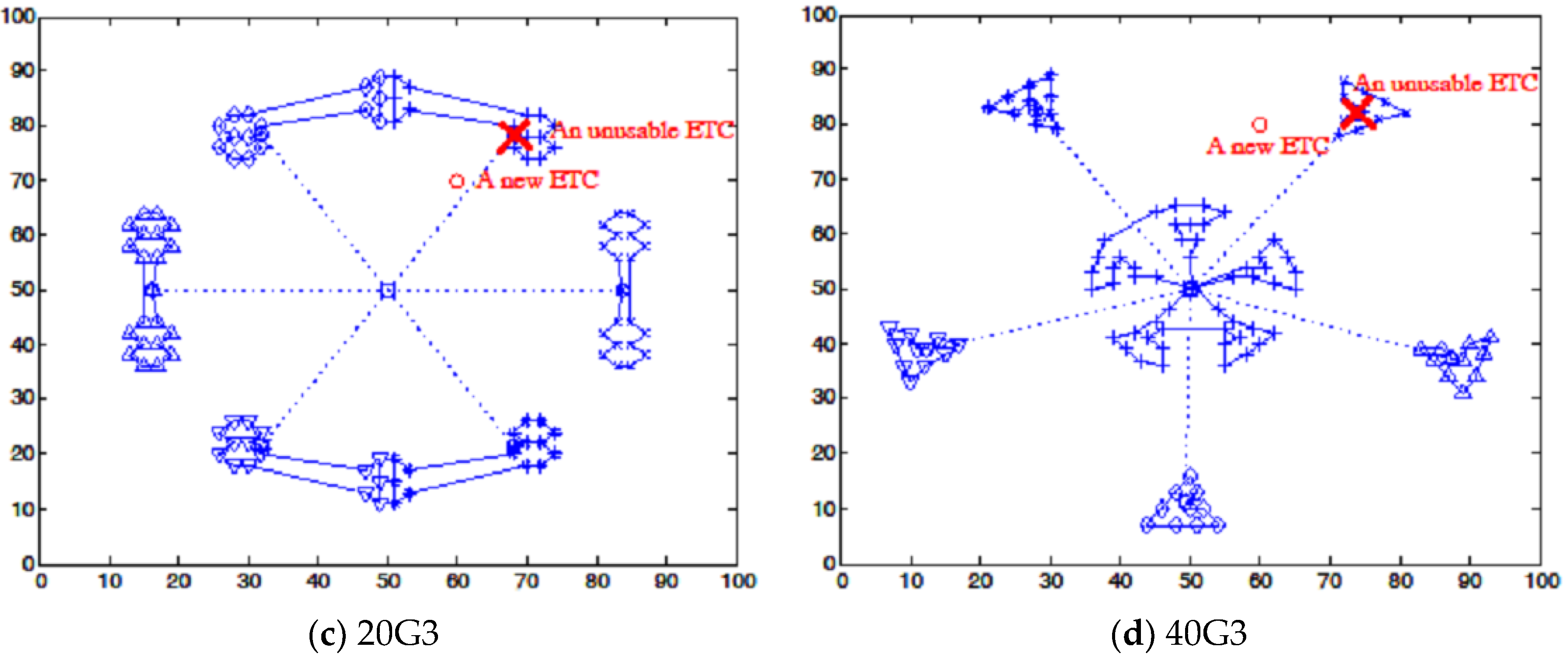
As mentioned above, the scenario of updated emergency transfer centers (ETCs) mainly included two categories: added ETCs and cancelled ETCs. Here, the authors consider the following disruption events for each emergency instance: One new ETC is added, and one extant ETC is cancelled. The detailed disruptions are as Figure 5 shows. The decision problem is to generate new intermodal routes in consideration of the disruption situation.
Subsequent to giving the original transportation routes and disruption situations, one can use the genetic algorithm (GA) based solving algorithm in Section 4 to produce recovered routes. During the implementation, the GA related parameters were set as follows: The population size was 25, the crossover probability was 0.9, and the mutation probability was 0.1. Based on the workload and cost analysis in general practical situations, the unit deviation penalties of helicopter route and quantity were often bigger than those of vehicle route and quantity, and the unit deviation penalty of the relief arrival time was relatively smaller. Thus, the disruption penalty parameters , , , and were set as 1, 100, 10, 100 and 30, respectively.
Since the disturbance was considered from three aspects, the recovered intermodal routes were probably different with different weights. Table 1 and Figure 6 show the recovered results with equivalent weights (the authors selected out the optimal recovered plan from five running results considering the randomness of the genetic algorithm). To show the advantage of this disruption management method, the authors obtained the recovered plan using the rescheduling method [20].
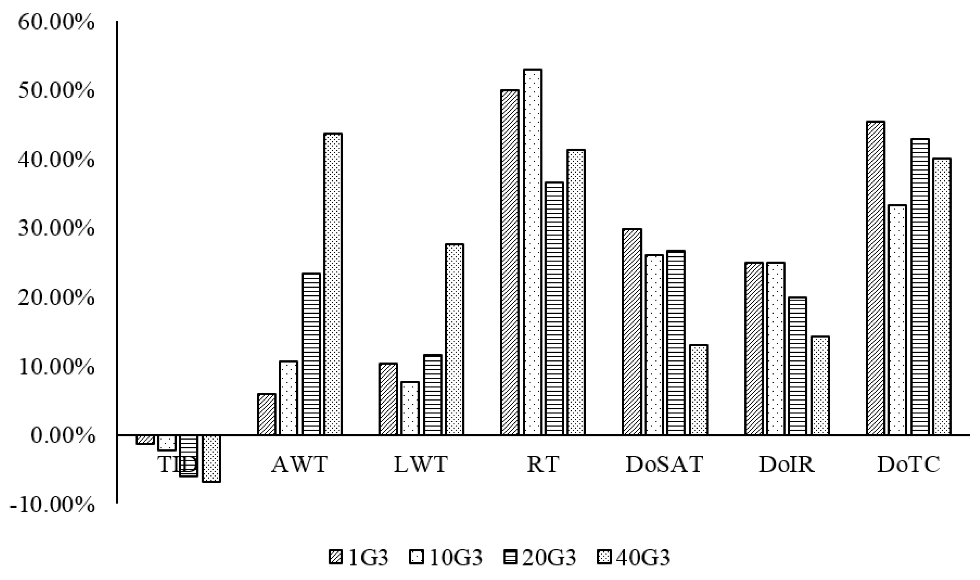
The total intermodal duration, average waiting time, and longest waiting time of the recovered intermodal delivery plan 1G3 were 1239.12, 108.86 and 210.55, respectively; they were 1021.32, 78.69, and 186.27 for 10G3; regarding 20G3, they were 530.37, 41.65, and 88.76; concerning 40G3, they were 440.60, 20.20, and 41.98. To compare with the original plan, the disturbance of supply arrival time was 216.24, 185.20, 154.32 and 120.25, the disturbance of intermodal routes was 220, 190, 180 and 160, and the disturbance of transportation capacity was 60, 60, 40 and 30. The result comparison between the disruption management method and the rescheduling method is as Table 1 and Figure 6 show. Taken from the comparison, the following observations can be made:
(i) Although the total intermodal duration of the recovered plans by the disruption management method was a little longer than those of the recovered plans by the rescheduling method, both the average waiting time and longest waiting time of the former were shorter than those of the latter.
(ii) Compared to the original plan, the disturbances of the supply arrival time, intermodal routes and transportation capacity of the recovered plan by the disruption management method were smaller than those of the recovered plan by the rescheduling method. This shows the advantage of the disruption management method in dealing with unexpected events.
(iii) The running time of the rescheduling method was longer than those of the disruption management method. This was probably because the rescheduling method needed to re-search the whole solution space to produce the recovered plan but the disruption management method only searched part of the solution space. The disruption management method was more suitable to emergency situations since it could narrow the solution space of the recovered routes.
Taken from the above comparison, the disruption management method can produce a recovered intermodal delivery plan with minimum disturbance to original plans in a short time. However, the rescheduling method only aims at minimizing the intermodal transportation duration with no consideration of the disturbance to the original plans, and thus often produces a recovered plan with large disturbance to the original plans.
6.3. Insights
As stated above, the selected four instances represent four kinds of residential space structures. Most big cities are, to some extent, similar to the former two instances, 1G3 and 10G3, and most rural/mountainous areas are to some extent similar to the latter two instances, 20G3 and 40G3. Findings and insights useful to support real-world disaster responses can be obtained, as Table 2 summarizes:
- Seen from the comparison of total intermodal duration (TID) in Figure 6, the disruption management method is more effective in uniform residential areas, that is, more suitable in city areas. Thus, if disasters happen in city areas, the disadvantage of this work over the rescheduling method is weakened.
- Considering average waiting time (AWT) and longest waiting time (LWT), the disruption management method can produce better performances in rural and mountainous areas than in city areas. This competitiveness shows that the intermodal transportation is more effective in scattered residential regions. When disasters happen in rural and mountainous areas, the intermodal transportation and the disruption management method are more advantageous.
- This study’s method shows obvious advantages over the rescheduling method in both cities and rural/mountainous villages. This competitiveness is because the disruption management method, and its corresponding genetic algorithm, effectively, can reduce the solution space by simplification strategy and genetic operations. Most emergency decision-makers might prefer this method due to the need for urgency in response to disasters.
- Regarding the disturbance of supply arrival time (DoSAT) and the disturbance of intermodal routes (DoIR), the current work is more suitable in city areas. When medical aid points (MAPs) were in uniform distribution, the change of emergency transfer centers (ETCs) had less impact on the arrival time and transport routes; When MAPs were in clustered villages, the change of ETCs had more impact. The impact extent is related to the advantage of the disruption management method.
7. Conclusions
The authors were concerned with the recovery of helicopter and vehicle intermodal transportation disturbed by updated emergency transfer centers. The disruption management idea was applied to deal with this problem. Specifically, the authors presented a disruption measurement method to quantify the impact of updated emergency transfer centers (ETCs) on intermodal transportation from three aspects: supply arrival time, intermodal routes and transportation capacity. The authors formulated a recovery model of intermodal transportation, aimed at minimizing the impact of updated ETCs on the original intermodal plan. To solve the recovery model, the authors used a genetic algorithm-type approach with a multilevel encoding method and simplification strategies. Using the algorithm, the disruption management idea also was applied. Experimental results showed the effectiveness and advantages of the disruption management method in comparison with the rescheduling method.
Although the disruption management idea is shown to be effective to adjust intermodal transportation plans when some emergency transfer centers are updated, there are still limitations in the work. First, the model does not fully consider the uncertainty in practical disaster responses. Besides the adding or cancelling of transportation nodes, there may be other kinds of uncertain situations in the iterative implementation of intermodal transportation plans. For example, transportation time and transfer time might not be as precise as was considered in the work. Second, the model only considers one kind of disruption event, updated ETCs, but other kinds of unexpected events, such as damaged vehicles, changed demands, spoiled supplies and surging resources, might happen separately or simultaneously with updated ETCs. Different recovery models will be required to deal with these different kinds of unexpected events. Meanwhile, the application of advanced techniques such as Internet of Things will have great impact on the emergency transportation [34]. Thus, future efforts should be made to extend this work, such as fuzzifying the model by setting the transportation time and transfer time as fuzzy numbers and considering the combination of multiple kinds of unexpected events.
Author Contributions
J.R. and F.T.S.C. designed the work; J.R. and X.Z. performed the experiments; F.T.S.C. contributed introduction/related studies; J.R. wrote the paper; F.T.S.C. proofread the paper.
Funding
This research was funded by [Natural Science Basic Research Project in Shaanxi Province] grant number [2016JQ7005], [Science and Technology Plan Projects of Yangling Demonstration Zone] grant number [2016RKX-04], the [Fundamental Research Funds for the Central Universities] grant number [2018RWSK02], and [The Hong Kong Polytechnic University Internal Project] grant number [G-UADM].
Acknowledgments
We gratefully acknowledge the anonymous referees for their constructive comments on the manuscript. We are so thankful to the English language editing by MDPI.
Conflicts of Interest
The authors declare no conflict of interest.
References
- Qin, J.; Ye, Y.; Cheng, B.-R.; Zhao, X.; Ni, L. The emergency vehicle routing problem with uncertain demand under sustainability environments. Sustainability 2017, 9, 288. [Google Scholar] [CrossRef]
- Yang, Z.; Guo, L.; Yang, Z. Emergency logistics for wildfire suppression based on forecasted disaster evolution. Ann. Oper. Res. 2017. [CrossRef]
- Mohammadi, R.; Fatemi Ghomi, S.M.T.; Jolai, F. Prepositioning emergency earthquake response supplies: A new multi-objective particle swarm optimization algorithm. Appl. Math. Model. 2016, 40, 5183–5199. [Google Scholar] [CrossRef]
- Zokaee, S.; Bozorgi-Amiri, A.; Sadjadi, S.J. A robust optimization model for humanitarian relief chain design under uncertainty. Appl. Math. Model. 2016, 40, 7996–8016. [Google Scholar] [CrossRef]
- Jin, S.; Jeong, S.; Kim, J.; Kim, K. A logistics model for the transport of disaster victims with various injuries and survival probabilities. Ann. Oper. Res. 2015, 230, 17–33. [Google Scholar] [CrossRef]
- Chen, A.Y.; Yu, T.-Y. Network based temporary facility location for the emergency medical services considering the disaster induced demand and the transportation infrastructure in disaster response. Transp. Res. Part B 2016, 91, 408–423. [Google Scholar] [CrossRef]
- Jia, H.; Ordóñez, F.; Dessouky, M.M. Solution approaches for facility location of medical supplies for large-scale emergencies. Comput. Ind. Eng. 2007, 52, 257–276. [Google Scholar] [CrossRef] [Green Version]
- Mete, H.O.; Zabinsky, Z.B. Stochastic optimization of medical supply location and distribution in disaster management. Int. J. Prod. Econ. 2010, 126, 76–84. [Google Scholar] [CrossRef]
- Su, Q.; Luo, Q.; Huang, S.H. Cost-effective analyses for emergency medical services deployment: A case study in Shanghai. Int. J. Prod. Econ. 2015, 163, 112–123. [Google Scholar] [CrossRef]
- Iannoni, A.P.; Morabito, R. A multiple dispatch and partial backup hypercube queuing model to analyze emergency medical systems on highways. Transp. Res. Part E 2007, 43, 755–771. [Google Scholar] [CrossRef]
- Ruan, J.H.; Shi, P.; Lim, C.C.; Wang, X.P. Relief supplies allocation and optimization by interval and fuzzy number approaches. Inf. Sci. 2015, 303, 15–32. [Google Scholar] [CrossRef]
- Erdemir, E.T.; Batta, R.; Rogerson, P.A.; Blatt, A.; Flanigan, M. Joint ground and air emergency medical services coverage models: A greedy heuristic solution approach. Eur. J. Oper. Res. 2010, 207, 736–749. [Google Scholar] [CrossRef]
- Ruan, J.H.; Wang, X.P.; Shi, Y. A two-stage approach for medical supplies intermodal transportation in large-scale disaster responses. Int. J. Environ. Res. Public Health 2014, 11, 11081–11109. [Google Scholar] [CrossRef] [PubMed]
- Ruan, J.H.; Wang, X.P.; Chan, F.T.S.; Shi, Y. Optimizing the intermodal transportation of emergency medical supplies using balanced fuzzy clustering. Int. J. Prod. Res. 2016, 54, 4368–4386. [Google Scholar] [CrossRef]
- Eckstein, M.; Jantos, T.; Kelly, N.; Cardillo, A. Helicopter transport of pediatric trauma patients in an urban emergency medical services system: A critical analysis. J. Trauma 2002, 53, 340–344. [Google Scholar] [CrossRef] [PubMed]
- Matsumoto, H.; Motomura, T.; Hara, Y.; Masuda, Y.; Mashiko, K.; Yokota, H.; Koido, Y. Lessons learned from the aeromedical disaster relief activities following the great East Japan earthquake. Prehosp Disaster Med. 2013, 28, 166–169. [Google Scholar] [CrossRef] [PubMed]
- Barbarosoğlu, G.; Özdamar, L.; Çevik, A. An interactive approach for hierarchical analysis of helicopter logistics in disaster relief operations. Eur. J. Oper. Res. 2002, 140, 118–133. [Google Scholar] [CrossRef]
- Özdamar, L. Planning helicopter logistics in disaster relief. OR Spectr. 2011, 33, 655–672. [Google Scholar] [CrossRef]
- Li, J.Q.; Borenstein, D.; Mirchandani, P.B. A decision support system for the single-depot vehicle rescheduling problem. Comput. Oper. Res. 2007, 34, 1008–1032. [Google Scholar] [CrossRef]
- Li, J.Q.; Pitu, B.M.; Denis, B. A Lagrangian heuristic for the real-time vehicle rescheduling problem. Transp. Res. Part E 2009, 45, 419–433. [Google Scholar] [CrossRef]
- Archetti, C.; Guastaroba, G.; Speranza, M.G. Reoptimizing the rural postman problem. Comput. Oper. Res. 2013, 40, 1306–1313. [Google Scholar] [CrossRef]
- Mu, Q.; Fu, Z.; Lysgaard, J.; Eglese, R. Disruption management of the vehicle routing problem with vehicle breakdown. J. Oper. Res. Soc. 2011, 62, 742–749. [Google Scholar] [CrossRef] [Green Version]
- Wang, X.P.; Ruan, J.H.; Shi, Y. A recovery model for combinational disruptions in logistics delivery: Considering the real-world participators. Int. J. Prod. Econ. 2012, 140, 508–520. [Google Scholar] [CrossRef]
- Hu, X.P.; Sun, L.J.; Liu, L.L. A PAM approach to handling disruptions in real-time vehicle routing problems. Decis. Support Syst. 2013, 54, 1380–1393. [Google Scholar] [CrossRef]
- Qi, X.T.; Bard, J.F.; Yu, G. Supply chain coordination with demand disruptions. Omega Int. J. Manag. 2004, 32, 301–312. [Google Scholar] [CrossRef]
- Xiao, T.; Yu, G.; Sheng, Z.; Xia, Y. Coordination of a supply chain with one-manufacturer and two-retailers under demand promotion and disruption management decisions. Ann. Oper. Res. 2005, 135, 87–109. [Google Scholar] [CrossRef]
- Sarkar, S.; Kumar, S. A behavioral experiment on inventory management with supply chain disruption. Int. J. Prod. Econ. 2015, 169, 169–178. [Google Scholar] [CrossRef]
- Bode, C.; Wagner, S.M. Structural drivers of upstream supply chain complexity and the frequency of supply chain disruptions. J. Oper. Manag. 2015, 36, 215–228. [Google Scholar] [CrossRef]
- Zhang, D.Z.; Zou, F.Z.; Li, S.Y.; Zhou, L.Y. Green supply chain network design with economies of scale and environmental concerns. J. Adv. Transport. 2017, 3, 1–14. [Google Scholar] [CrossRef]
- Yuan, J.J.; Mu, Y.D. Rescheduling with release dates to minimize makespan under a limit on the maximum sequence disruption. Eur. J. Oper. Res. 2007, 182, 936–944. [Google Scholar] [CrossRef]
- Ozlen, M.; Azizoglu, M. Rescheduling unrelated parallel machines with total flow time and total disruption cost criteria. J. Oper. Res. Soc. 2011, 62, 152–164. [Google Scholar] [CrossRef]
- Ahmadi, E.; Zandieh, M.; Farrokh, M.; Emami, S.M. A multi objective optimization approach for flexible job shop scheduling problem under random machine breakdown by evolutionary algorithms. Comput. Oper. Res. 2016, 73, 56–66. [Google Scholar] [CrossRef]
- Mohammadi, M.; Jolai, F.; Moghaddam, R.T. Solving a new stochastic multi-mode p-hub covering location problem considering risk by a novel multi-objective algorithm. Appl. Math. Model. 2013, 37, 10053–10073. [Google Scholar] [CrossRef]
- Ruan, J.H.; Wang, Y.X.; Chan, F.T.S.; Hu, X.P.; Zhao, M.J.; Zhu, F.W.; Shi, B.F.; Shi, Y.; Lin, F. A life-cycle framework of green IoT based agriculture and its finance, operation and management issues. IEEE Commun. Mag. 2018. [Google Scholar] [CrossRef]
Figure 1.
The focus problem in this work (LCDH represents the large collecting and distributing hub, ETCs represent emergency transfer centers, and MAPs represent medical aid points).
Figure 1.
The focus problem in this work (LCDH represents the large collecting and distributing hub, ETCs represent emergency transfer centers, and MAPs represent medical aid points).
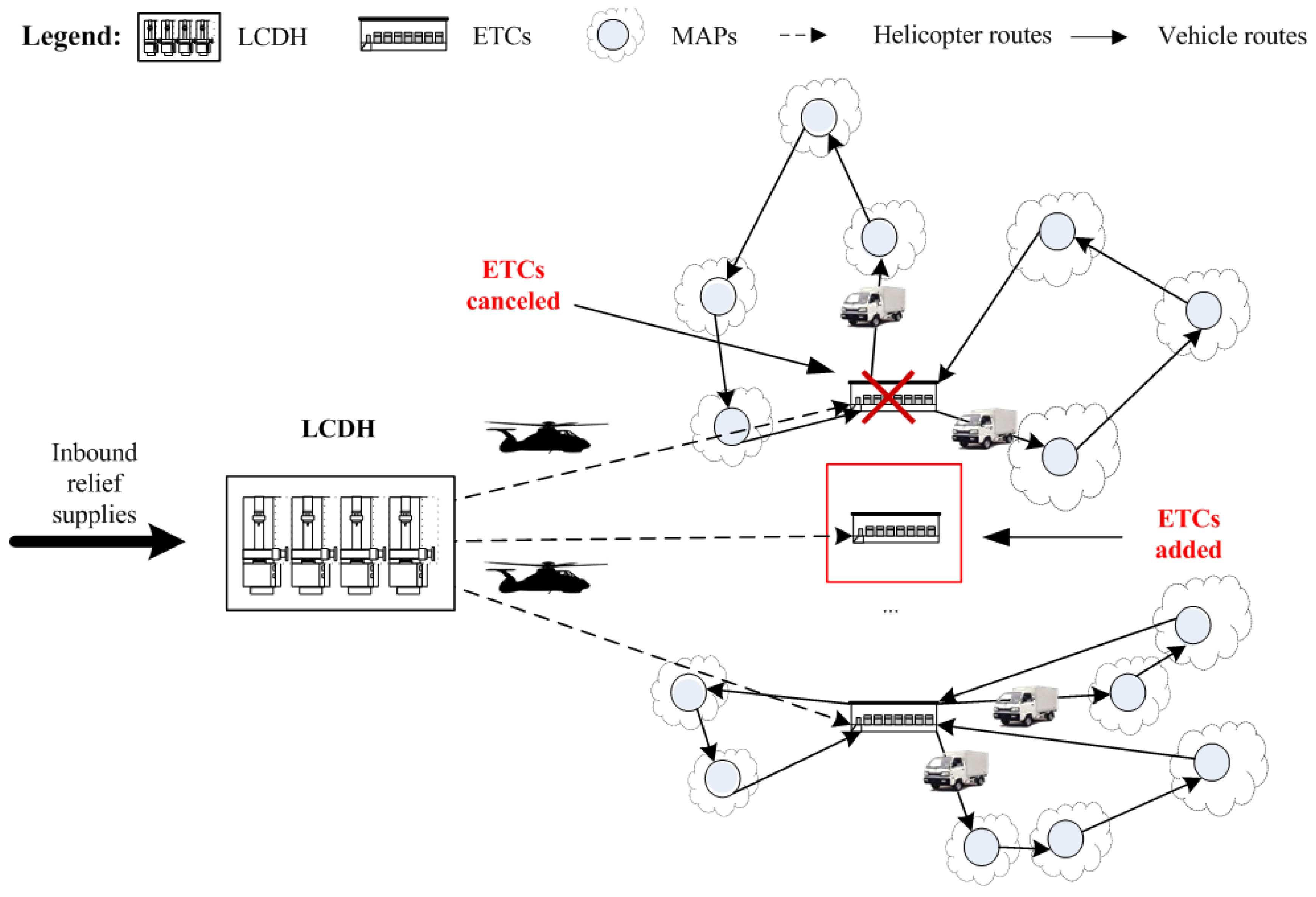
Figure 2.
An example of the multilevel encoding chromosome.
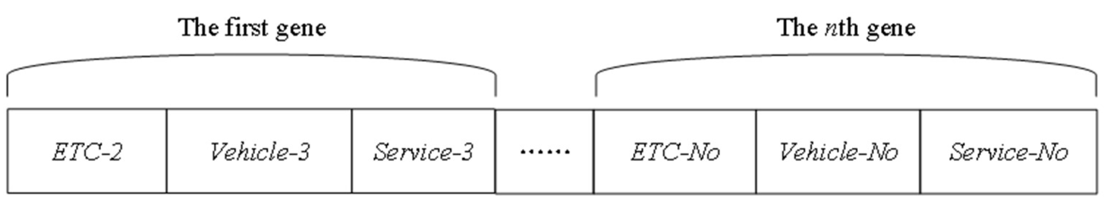
Figure 3.
The distributions of four emergency instances. (a) 1G3 in an ideal uniform structure; (b) 10G3 in a circular radial structure; (c) 20G3 in a scattered structure with no center; (d) 40G3 in a scattered structure with a central zone.
Figure 3.
The distributions of four emergency instances. (a) 1G3 in an ideal uniform structure; (b) 10G3 in a circular radial structure; (c) 20G3 in a scattered structure with no center; (d) 40G3 in a scattered structure with a central zone.
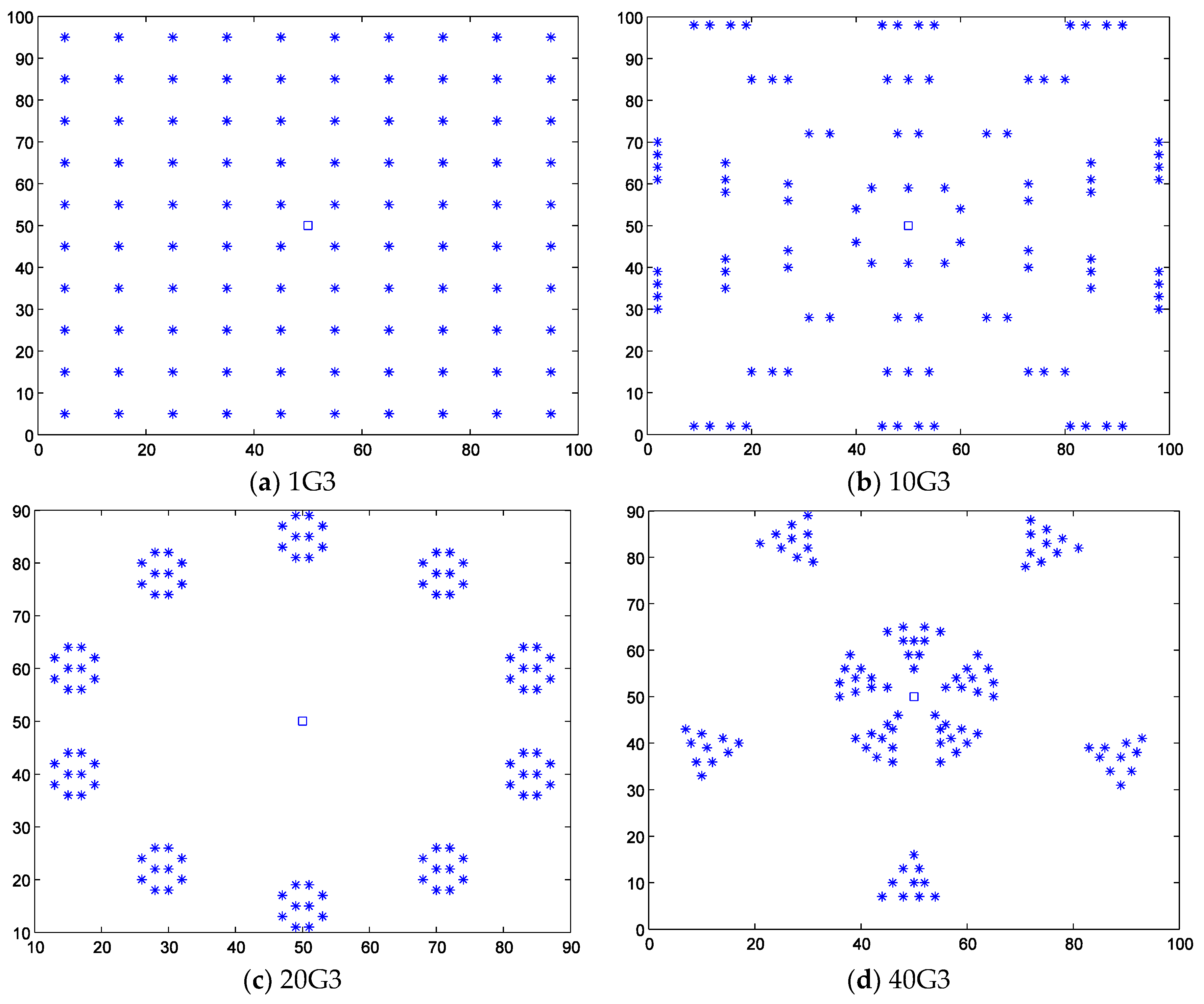
Figure 4.
Original intermodal plans (the dash lines represent helicopter routes and the solid lines represent vehicle routes). (a) The original intermodal plan of the 1G3 instance; (b) The original intermodal plan of the 10G3 instance; (c) The original intermodal plan of the 20G3 instance; (d) The original intermodal plan of the 40G3 instance.
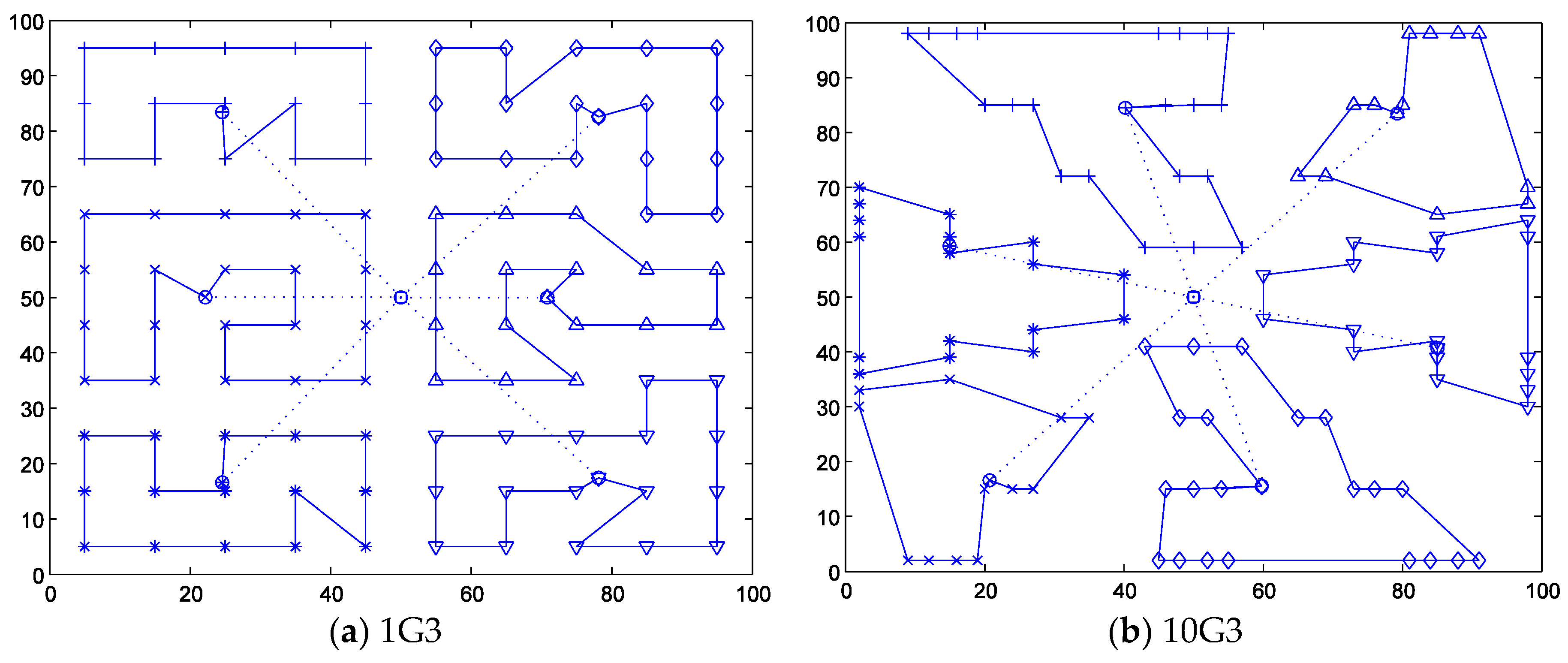
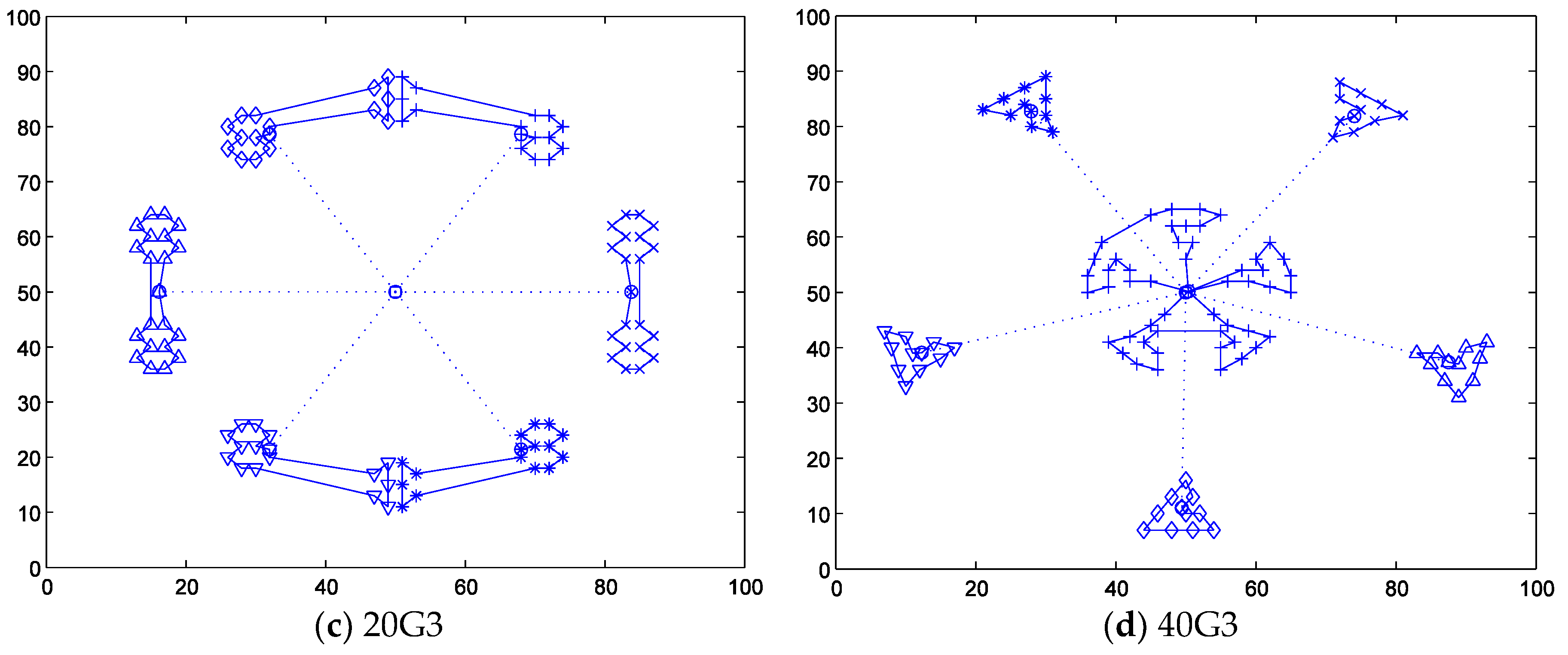
Figure 5.
The disruption situations (the dash lines represent helicopter routes and the solid lines represent vehicle routes). (a) The disruption situation of the 1G3 instance; (b) The disruption situation of the 10G3 instance; (c) The disruption situation of the 20G3 instance; (d) The disruption situation of the 40G3 instance.


Figure 6.
The improved performance of the disruption management method over the rescheduling method.
Figure 6.
The improved performance of the disruption management method over the rescheduling method.


Table 1.
The result comparison between the disruption management method and the rescheduling method (the bold values mean the better).
Table 1.
The result comparison between the disruption management method and the rescheduling method (the bold values mean the better).
| Instances | Performance Metrics | The Disruption Management Method | The Rescheduling Method |
|---|---|---|---|
| 1G3 | Total intermodal duration | 1239.12 | 1223.65 |
| Average waiting time | 108.86 | 115.68 | |
| Longest waiting time | 210.55 | 234.71 | |
| The running time | 8.28 | 16.55 | |
| The disturbance of supply arrival time | 216.24 | 308.17 | |
| The disturbance of intermodal routes | 220 | 160 | |
| The disturbance of transportation capacity | 60 | 110 | |
| 10G3 | Total intermodal duration | 1021.32 | 998.15 |
| Average waiting time | 78.69 | 88.10 | |
| Longest waiting time | 186.27 | 201.86 | |
| The running time | 7.47 | 15.89 | |
| The disturbance of supply arrival time | 185.20 | 250.42 | |
| The disturbance of intermodal routes | 190 | 120 | |
| The disturbance of transportation capacity | 60 | 90 | |
| 20G3 | Total intermodal duration | 530.37 | 500.18 |
| Average waiting time | 41.65 | 54.35 | |
| Longest waiting time | 88.76 | 100.42 | |
| The running time | 5.40 | 8.52 | |
| The disturbance of supply arrival time | 154.32 | 210.64 | |
| The disturbance of intermodal routes | 180 | 100 | |
| The disturbance of transportation capacity | 40 | 70 | |
| 40G3 | Total intermodal duration | 440.60 | 412.14 |
| Average waiting time | 20.20 | 35.89 | |
| Longest waiting time | 41.98 | 58.01 | |
| The running time | 6.11 | 10.42 | |
| The disturbance of supply arrival time | 120.25 | 138.32 | |
| The disturbance of intermodal routes | 160 | 70 | |
| The disturbance of transportation capacity | 30 | 50 |
Table 2.
The more effective areas of this work.
| Metrics | City Areas (1G3 and 10G3) | Rural and Mountainous Areas (20G3 and 40G3) |
|---|---|---|
| Total intermodal duration (TID) | √ | |
| Average waiting time (AWT) | √ | |
| Longest waiting time (LWT) | √ | |
| The running time (RT) | √ | |
| The disturbance of supply arrival time (DoSAT) | √ | |
| The disturbance of intermodal routes (DoIR) | √ | |
| The disturbance of transportation capacity (DoTC) | No effective areas | |
© 2018 by the authors. Licensee MDPI, Basel, Switzerland. This article is an open access article distributed under the terms and conditions of the Creative Commons Attribution (CC BY) license (http://creativecommons.org/licenses/by/4.0/).
Share and Cite
MDPI and ACS Style
Ruan, J.; Chan, F.T.S.; Zhao, X. Re-Planning the Intermodal Transportation of Emergency Medical Supplies with Updated Transfer Centers. Sustainability 2018, 10, 2827. https://doi.org/10.3390/su10082827
AMA Style
Ruan J, Chan FTS, Zhao X. Re-Planning the Intermodal Transportation of Emergency Medical Supplies with Updated Transfer Centers. Sustainability. 2018; 10(8):2827. https://doi.org/10.3390/su10082827
Chicago/Turabian StyleRuan, Junhu, Felix T. S. Chan, and Xiaofeng Zhao. 2018. "Re-Planning the Intermodal Transportation of Emergency Medical Supplies with Updated Transfer Centers" Sustainability 10, no. 8: 2827. https://doi.org/10.3390/su10082827
Note that from the first issue of 2016, this journal uses article numbers instead of page numbers. See further details here.