Assessment of Agri-Environmental Externalities in Spanish Socio-Ecological Landscapes of Olive Groves

Abstract

Traditional agricultural systems and their spatial context constitute socio-ecological landscapes for their long co-evolutionary history. However, these systems not only generate positive but also negative agri-environmental externalities, such as soil erosion, diffuse pollution and potential wild biodiversity degradation. In this paper, we present a methodological approach for developing and testing indicators to estimate the effects of these externalities, especially designed to be used to help guide land-use policy changes. Our results show that the indicators proposed can recognize the different environmental situations posed by the three selected study areas, in terms of potential erosion and diffuse pollution, as well as in the actual agri-environmental externalities assessment. As expected, they also respond to the changes in land use and management introduced by two scenarios, ecological and productive. Although the erosion and diffuse pollution indicators showed a linear response, the diversity indicator showed a non-linear response, which highlights the importance of the spatial structure of landscape in agri-environmental assessment. In fact, several ecological processes can be affected by landscape spatial structure, potentially giving unexpected results both in terms of indicators and of real impact of agri-environmental externalities. Therefore, some landscape structure assessment should accompany that of externalities when considering land-use policy objectives.

1. Introduction

Historically, the essential role of agriculture has been the provision of food. However, in recent years, its multifunctional value to society has been assumed [1]. This means that in addition to producing food, it must also contribute to economic and social development. In addition, at present the way that food is produced and consumed is vital for a sustainable food future. Therefore, one of the greatest global challenges is to increase agricultural production reducing its current impact on climate, water, and ecosystems, and maintaining the supply of ecosystem services (i.e., soil productivity, water purification, carbon uptake, landscape quality) and biodiversity [2]. In the European Union (EU), the Common Agricultural Policy (CAP) is the key element to determine rural policies for agriculture and environmental management [3]. The early stages of CAP implementation in the 1960s were especially focused on two aspects: farm income through a system of fixed common price, and agricultural production efficiency through structural changes in traditional farms [4]. This productivist and economic-oriented agricultural approach had a direct impact on agriculture management. Farmers intensified their management with the undesirable side-effect of increasing pressure on the environment. For this reason, CAP reforms since 1992 have aimed to progressively reduce the pressure of agriculture on the environment. Specifically, the changes could be described as a sequential evolution from a productivity phase between the 1960s to the 1980s; a competitiveness phase from the 1980s to the 1990s; and a sustainability phase from the 1990s to the present [5].

Several instruments and tools have been developed and made available to farmers to mitigate the environmental impact of agriculture. Agri-environment schemes (AES), one of these policy tools, provide financial support for the EU countries to design and implement different agricultural and environmental measures. The environmental measures, that involve paying to farmers who adopt specific environmental management practices, include organic farming, integrated production, reducing inputs (i.e., fertilisers and pesticides), crop rotation, maintaining habitats for wildlife, introducing buffer strips, and conserving genetic resources in agriculture. Currently, close to 25% of the EU’s agricultural area is under AES contracts with farmers. However, several authors corroborate farmer resistance to AESs [6] or are skeptical about the success of AES objectives [7]. In this sense, a recent report [8] evaluates the results and adaptation of EU Rural Development Programmes, which constitute the second pillar of the EU’s CAP. This report emphasizes the importance of conducting periodic assessments at different levels (e.g., the national level) to detect deficiencies in the existing laws and measures related to rural development and, consequently, to identify what can be improved or simplified in order to achieve the stated objectives. In other words, there should be a feedback between evaluations and policies in order to improve the measures, standards and objectives for rural development.

In this sense, the “sustainability phase” would take into account the evidence for landscape effects on ecological and farming systems [9,10], opening the way for AES to be implemented at a landscape level. This means preserving also the rural landscapes from which they come, highly valued by society in areas where “natural” ecosystems have a long history of coexistence with agroecosystems [11]. Moreover, this scale would be the basis for the planning of the objectives of rural development, and farming systems should be considered in the context of rural landscapes. The functionality of these landscapes depends on the interactions among natural ecosystems, agroecosystems, and the social and cultural characteristics of the people that create and manage them [12]. Therefore, rural landscapes constitute socio-ecological landscapes, not only of high environmental and economic value, but also with important social and aesthetic functions [13], i.e., they produce a series of externalities, both positive and negative. Besides high-quality products, the viability of rural areas, maintenance of rural population and provision of cultural and aesthetic services are among the positive socio-economic externalities. Different environmental benefits derive from them, such as the regulation of ecological processes, or provision of new or intermediate habitats for many species. However, important negative agri-environmental externalities can also be detected associated with these systems, usually grouped by the affected media, i.e., soil, air and water, together with biodiversity and landscape [12,13]. Soil degradation, erosion or contamination, greenhouse gas emissions, water pollution or eutrophication, are some of the potential environmental effects associated with agriculture. In addition, local and regional biodiversity can be affected in a negative way, as well as different properties of landscapes, which in turn could jeopardize the provision of goods and services of socio-ecological landscapes. Soil degradation by runoff is one of the most important processes in the loss of land productive capacity [14]. Pollution from diffuse agricultural sources is the main cause of deterioration of surface freshwater and groundwater quality affecting drinking water supplies and contributing to the process of eutrophication [15]. In relation to biodiversity, its current rate of loss is considered an environmental risk at the planetary scale, and even dangerous for human well-being [16]. If more complex and, therefore, better decisions are to be taken, the agri-environmental externalities should be properly quantified and incorporated in the framework of a cost-benefit analysis of the public or private decisions of society [17]. In this context, the quantification of the negative externalities associated with farming systems at the landscape scale is crucial and requires adequate indicators [18].

The Spanish socio-ecological landscape of olive groves, due to its extent, economic importance, cultural and social values, and data available, constitutes a paradigmatic case study in which to define and test the performance of indicators for these environmental externalities. Despite its obvious relevance at the national level, paradoxically it has produced very few quantitative studies [19,20,21]. In addition, at the regional level, the Regional Government of Andalusia has enacted the Andalusian Act for the Olive Grove (2011) and corresponding financial allocation through the Master Plan (2015). Specifically, it established financial support for farmers that apply herbaceous ground cover and the preservation of stone walls and hedges to reduce soil erosion, increase water retention, and benefit biodiversity. Quantification of the negative externalities would allow assigning correctly these economic supports along with other local or regional payments. Therefore, given the growing interest in quantifying environmental externalities to minimize their negative impacts on production and improve profitability for farmers, the development of objective indicators of these externalities has become essential. With this in mind, the aims of this paper are:

• To propose indicators to adequately assess the impact of the agri-environmental externalities of soil erosion, diffuse pollution and biodiversity, at a landscape level.
• To illustrate their performance by proposing scenarios of possible changes in olive grove management for two olive oil Protected Denominations of Origin (PDOs).

2. Materials and Methods

2.1. Agri-Environmental Indicators

The European Environment Agency (EEA) defines an indicator as “a measure, generally quantitative, that can be used to illustrate and communicate complex environmental phenomena simply, including trends and progress over time—and thus helps provide insight into the state of the environment” [22]. The pioneering work of the Organisation for Economic Co-operation and Development (OECD) set the criteria for indicator selection [23]. Both from the EEA definition and the OECD criteria, we highlight several characteristics as leading criteria to organise and propose a conceptual framework [24] for selecting environmental indicators to be used as a guide in land planning and socio-ecological landscape management. These should be:

• Quantitative [22], and in equation form, to be computable for each specific situation or case study (which complies with “being either national in scope or applicable to regional environmental issues of national significance” [23]).
• Be simple, easy to interpret [23], (i.e., based on “canonical”, not synthetic or compound) variables. To “communicate complex environmental phenomena simply” [22], those variables should be related to clear physical or biological processes.
• Straightforward, of easy interpretation, and if possible they should enable the assessment of potentialities or risks as well as, or rather than, net quantities. In other words, whenever possible they should distinguish between the physical or ecological properties of the environmental systems in which socio-cultural landscapes develop, and the variable part, specific (and more contingent) entities such as land-cover/land-use types. In this way, “their response to changes in the environment and related human activities” [23] would be made more clear, and the structure would better accommodate hypothesis testing (e.g., comparing alternative scenarios of change by “linking indicators to economic models, forecasting and information systems” [23]).
• Appropriate to the scale and resolution of initial data. To be useful in the context of productive systems, indicators must be calculated at the appropriate spatial scale, set by the size of the most abundant individual production unit. Depending on the externality assessed, indicators calculated at a coarser scale could render an image too fuzzy to be considered as a basis for management. In addition, depending on the use to be given to the indicators, initial data resolution is highly relevant. Bottom-up approaches such as those revised by Payraudeau and van der Werf [25], in which data are directly obtained from individual exploitation units, can be costly and very time consuming. Top-down as well as bottom-up approaches are needed to reach the desirable integration between land planning and socio-cultural landscape management. An appropriate selection of compatible indicators calculated for each approach, based on initial data referring to common “canonical” processes, could help in this.

Needless to say, the remaining characteristics stated by the OECD [23] (e.g., “be theoretically well-founded in technical and scientific terms”, “have a threshold or reference value”, “be based on international standards”, “provide a basis for international comparisons”) can be derived from these leading criteria.

On the other hand, our three agri-environmental externalities—soil erosion, diffuse pollution and biodiversity—can be associated with existing agri-environmental indicators among those proposed by the European Commission [26], with varying degrees of compliance with framework criteria and aims. For soil erosion the use of the Revised Universal Soil Loss Equation (RUSLE) is proposed, which directly measures soil loss by runoff, and thus fully fits into the framework. However, in the case of diffuse pollution, among the several indicators (Risk of pollution by phosphorus, Pesticide risk, Mineral fertiliser consumption, Consumption of pesticides, Gross nitrogen balance) some are not fully developed (Pesticide risk), or do not fully match the stated framework (e.g., in spatial scale, data availability) or aim (see discussion below about the source and sink issue) under its present definition. Similar considerations could be made about those related to biodiversity (Agricultural areas under Natura 2000, High nature value farmland, Population trends of farmland birds, Landscape state and diversity).

In this context, we propose the following indicators, which according to the details stated in each section below must be considered proxy indicators [24]:

Soil erosion: In accordance with the EEA, we propose for our framework the RUSLE [27] as the soil erosion indicator. Although calculations of soil erosion using an improved version of the RUSLE have been made for the EU, at a spatial scale of 1 ha (RUSLE2015 [26]), as our framework demands, it is not available for Spain. Therefore, we need to calculate soil erosion for this paper, with the following equation:

ErI = [R·K·LS]·[C·P]

(1)

where ErI is the annual soil loss in t·ha⁻¹·yr⁻¹. This equation is widely used and meets criteria 1, 2 and 3 (square brackets differentiate between physical and variable parts). Its detailed consideration of all processes involved in soil erosion by runoff, however, implies the need for data that cannot be obtained without an appropriate sampling at farm level, mainly regarding soil properties and management practices. Therefore, to meet criterion 4 we made some simplifications regarding factors K and C. The soil erodibility factor (K), given the lack of a general consistent soil cartographic database for the whole of Spain, was derived from the parent material (geologic map 1:50,000, [28]), using tables from [29] and expert confirmation. For the cover management factor (C), we used general tables compiled by the Nature Conservation Institute [30]. As regards the remaining parameters, the rainfall erosivity factor R was obtained from the Spanish Meteorological Agency, and the slope length and steepness factor LS was calculated following the method of McCool et al. [31] and the Calsite approximation [32] for λ calculation. Computation of the first part gave the Potential Erosion Map (considered invariable at short time scales as it depends only on climatic, geologic and topographic variables), and its combination with factors C and P (support practices factor) the final value for the erosion indicator, the Estimated Erosion Map.

Diffuse pollution: Diffuse pollution has three components according to the paths pollutants can take: atmospheric, land surface and subterranean. Given the complexities inherent to atmospheric and subterranean circulation models, we concentrate on pollution carried by runoff fluxes. In addition, the problem of diffuse pollution in a given piece of land can be considered from two viewpoints, sink or source of pollutants. In our context of agri-environmental externalities, the detection of areas with a high risk of becoming strong sources of pollutants is a priority. Most indicators are devised to assess diffuse pollution in target areas from the sink perspective, by collecting data from a framework of assessment stations. This is the proper thing to do to evaluate the result of pollution-control policies, but it is not enough when designing policies and focusing measures on specific territories and landowners. Thus, we propose the following indicator:

DPoI = [(1-I)·Rt·Ar]·[Po]

(2)

where the physical part is mainly a function of runoff (as a fraction, 1-I) and the area to which that runoff can reach (downslope watershed, Ar). I represents the infiltration rate, calculated as a function of slope (Slp):

I = Pe·Exp(−0.041·Slp)

(3)

This was derived from a regression function (R² = 0.98) adjusted to the relativized data provided by the experiments of Nassif and Wilson [33].

The edaphic parameters, permeability (Pe, Equation (2)) and pollutant retention coefficient (Rt, Equation (1)), take into account the different characteristics of substrate, and were derived from the geologic map as proportions (0–1). The proportion (%) of total area affected by emissions on a given territory unit (Ar) was computed as the surface area of the downslope watershed in ha, and relativized by the total area considered in the study.

The physical part resulted in a Potential Diffuse Pollution Map, to which the variable part (pollutant emission from each territory unit, Po) was incorporated to get a final Diffuse Pollution Emission Risk Map. Within the proposed conceptual framework, this final map could be specific for a given pollutant (organic such as any given pesticide, or mineral such as N or P), if the appropriate parameters (regarding half life or degradation/metabolism rates, water solubility, interaction with substrate, etc.) are incorporated in the indicator’s equation. Indicator units would then be pollutant net quantities, mass or concentration, depending on input units. Conversely, the final map could be a general one if, for example, the aim is the detection of critical source areas where the use of agro-chemicals should be discouraged, or when comparing management practices for a given crop type, for which treatments can vary in number and/or intensity but not composition. This is the case illustrated in this paper, in which pollutant emission is quantified as the number of agro-chemical treatments involved in each olive grove type [34]. Consequently, in our case the DPoI has no units. If no agro-chemical treatment is applied, although the indicator would give a 0 value, this would only mean the return to the basal situation, in which a certain amount of soil content (N, P, etc.) is transferred between ecosystems/land-covers.

Biodiversity: Impact assessment of agriculture on biodiversity is an issue of great relevance [35] but also difficult to address at landscape scale, due to the extremely high diversity of taxonomic groups, life forms, body sizes, biological cycles, home ranges and dispersion distances involved, making it unmanageable to quantify without extensive and multidisciplinary sampling at farm level. That is, from the ecological point of view biodiversity at landscape scale should be addressed considering as many biological groups as possible, not only birds (as the Population trends of farmland birds indicator does), and also all land-use/land-cover types, not only agricultural ones (as the Agricultural areas under Natura 2000, High nature value farmland, Landscape state and diversity indicators do). Due to the problem of data availability, the usual approach in landscape ecology is to quantify diversity of land-cover types by means of different landscape metrics, based on the scientifically grounded principle that each land-cover type has its own cohort of species. In this way, a greater biodiversity can be inferred from a greater number of land-cover types (habitat diversity and matrix effects, see [36]). Broadly, natural and semi-natural land covers are considered as reservoirs for potential restoration and as refuges (and habitats), as well as stepping stones for wild and agriculturally sensitive species, beneficial to the biodiversity of an area [37,38]). Following this approach, we chose the Interspersion and Juxtaposition Index (IJI) [39] as a spatial diversity index:

$$\mathrm{DvI}=100·\left[{\displaystyle \sum }_{\mathrm{i}=1}^{\mathrm{m}}{\displaystyle \sum }_{\mathrm{k}=\mathrm{i}+1}^{\mathrm{m}}\left[\left({\mathrm{e}}_{\mathrm{ik}}/\mathrm{E}\right)\right]·\ln \left({\mathrm{e}}_{\mathrm{ik}}/\mathrm{E}\right)\right]/\ln \left(0.5·\left[\mathrm{m}·\left(\mathrm{m}-1\right)\right]\right)$$

(4)

where m is the number of land-cover types in the landscape, e_ik is the length of edge between uses i and k (i.e., contact), and E is total edge length in the landscape. This index is based on information theory, and is analogous to the Shannon–Wiener index of diversity [40], but instead of relative abundance of species, it computes relative abundance of edges between pairs of land-cover types. In this way, a landscape composed of a patch surrounded by only another land cover, would attain the lowest value (0), while a landscape composed of several patches, each one belonging to a different land-cover type and equally in contact with the rest of patches (equal edge length) would reach the maximum value (100). The IJI index was chosen instead of other indices because it considers explicitly edge length between pairs of land covers, which can be considered as a measure of probability of species interchange.

2.2. Study Area

In Spain, the production of olive oil from (mainly) monospecific stands of Olea europaea L., has a great economic importance (olive oil contributes €5600 million, almost 6% of the total production of the Spanish agro-food industry) and territorial extent (approximately 2,600,000 ha). Olive crops have historically been exploited in rain-fed extensive regimes in all types of terrains (even on sloping land), with the Andalusia region being the main area occupied by these crops [41,42]. The Spanish olive oil socio-ecological landscapes have an essential multifunctional role: a multi-habitat agricultural landscape with high values of biodiversity [43], a basic component of the economy representing close to 10% of national agricultural income, and a social cohesion factor, considering that more than 10% of the agricultural sector is employed in olive crops [44].

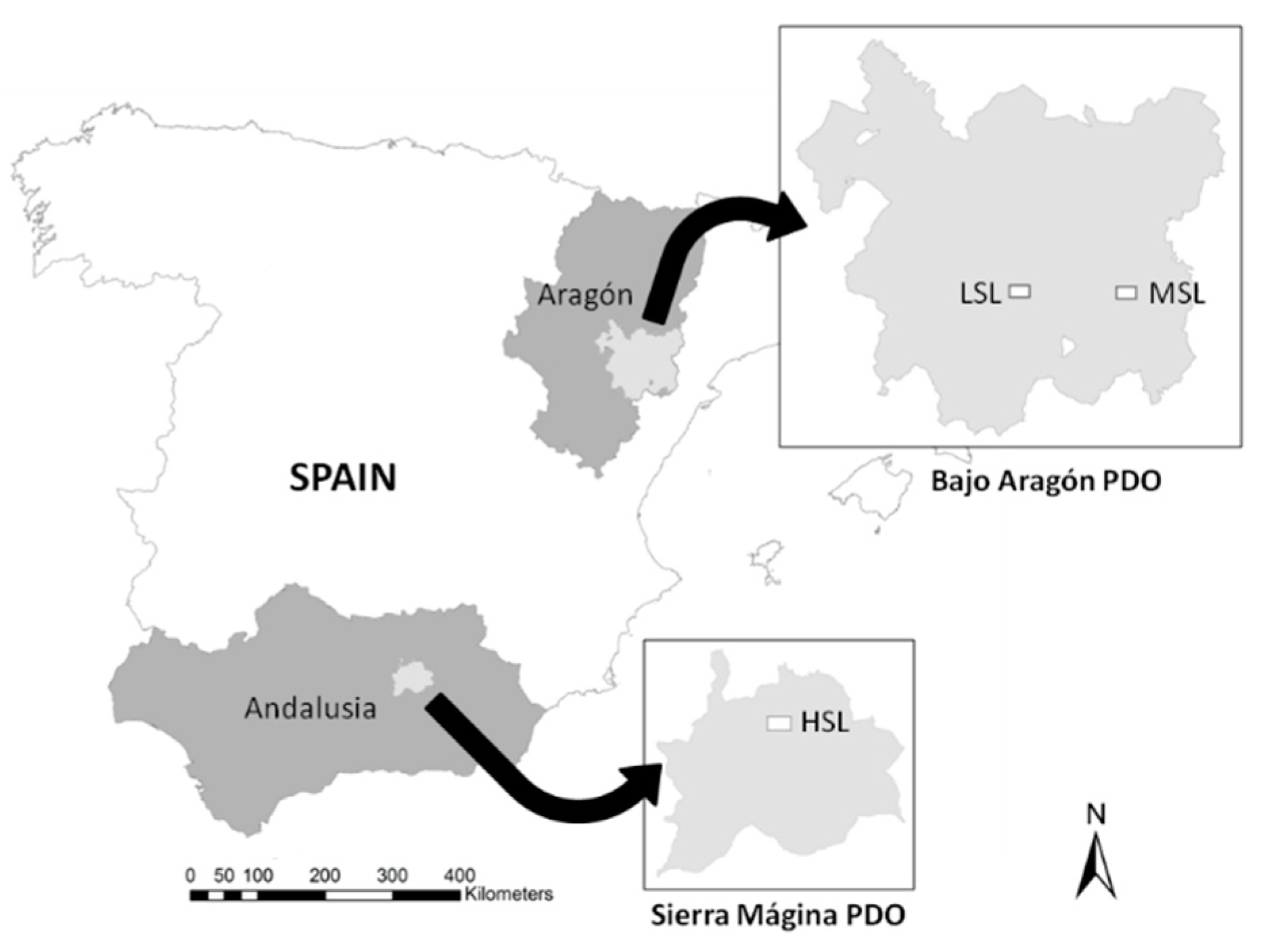
Two Protected Designations of Origin (PDOs) were selected to illustrate the performance of the agri-environmental indicators proposed. The first one, Sierra Mágina, is located in Jaén province (Andalusia, southern Spain, Figure 1), the main olive oil productive region in Spain. It has a continental Mediterranean climate with mountain influence, with mean annual temperature of 14.7 °C, and mean annual precipitation of 530.5 mm. Sierra Mágina comprises nearly 150,000 ha, with 60,000 ha devoted to olive groves, mainly on sloping land (>15%) due to its mountainous character, with a quite even distribution of rain-fed and irrigated olive groves. Inside the PDO is located the Sierra Mágina Natural Park, an area of 19,960 ha that includes the main ecosystems associated to its altitudinal gradient. The second one is Bajo Aragón, located to the north-east of Spain (Figure 1). It has a continental Mediterranean climate, with mean annual temperature of 15.9 °C and mean annual precipitation of around 417 mm. Bajo Aragón comprises more than 627,000 ha of medium to low slope terrain, mainly devoted to agriculture and pasture. Olive groves are not as widespread as in Andalusia (just 45,000 ha, less than 10%), and management practices and history are also somewhat different. From these PDOs three rectangular windows of 5 × 3 km were selected to have three different situations of olive grove cultivation: a high slope landscape (HSL, from Sierra Mágina); a medium slope landscape (MSL, from Bajo Aragón) corresponding to the region of Matarraña, often compared to the Italian Tuscany in relation to geomorphology and olive grove cultivation; and a low slope landscape (LSL, from Bajo Aragón).

2.3. Data Collection and Analysis

The base map for all analyses was the Spanish Land Registry Office map (Catastro), the official cartography of non-urban properties, as the land unit for olive grove management is the estate. Information on land-cover/land-use types was obtained from two datasets: for Sierra Mágina, the Andalusian Map of Land-Use and Vegetation Cover (MUCVA), and for Bajo Aragón the Spanish System of Land Occupation (SIOSE) map. To make both areas comparable, the SIOSE was reclassified into the categories of MUCVA, and the information of both datasets subsequently transferred to the Catastro base map. A slope map was derived from the 5-m resolution digital elevation model (DEM), and a slope mean value assigned to each polygon in the base map. The environmental data were completed with RUSLE factors C and P, obtained as explained above and assigned to each land-use type.

Estates devoted to olive cultivation were confirmed using official data [45], and their current number of olive trees was incorporated to the base map. Polygons were then classified according to slope and olive density into the olive grove types defined by the Spanish Association of Olive grove Municipalities ([34]; see

Table 1. Olive grove types in the study areas (HSL, MSL and LSL: high, medium and low slope landscape), according to the criteria of the Spanish Association of Olive grove Municipalities (AEMO). AEMO code: OTNMS = Sloped traditional rain-fed olive groves; OTMS = Traditional rain-fed olive groves; OIS = Intensive rain-fed olive groves; OISP = Sloped intensive rain-fed olive groves; OTNMR = Sloped traditional irrigated olive groves; OTMR = Traditional irrigated olive groves; OIR = Intensive irrigated olive groves; OIRP = Sloped intensive irrigated olive groves; OES = Ecological rain-fed olive grove; OER = Ecological irrigated olive groves.

	AEMO Characteristics			Olive Grove Types in the Study Areas
Landscapes	Code	Slope Range (%)	Density of Olive Trees	Area (ha)	% Total Area	% Olive Grove Area	Olive Trees/ha (x ± SD)	Slope (x)
HSL	OTNMS	≥20	<200	195.03	13.00	17.08	132.79 ± 31.51	32.02
	OTMS	<20	<200	191.46	12.76	16.77	121.6 ± 28.42	13.47
	OIS	<20	200–1000	2.08	0.14	0.18	229.21 ± 26.28	14.57
	OISP	≥20	200–1000	3.04	0.20	0.27	233.67 ± 42.69	36.47
	OTNMR	<20	<200	309.96	20.66	27.15	132.45 ± 32.37	28.37
	OTMR	<20	<200	424.65	28.31	37.20	124.35 ± 28.95	13.67
	OIR	<20	200–1000	7.68	0.51	0.67	233.28 ± 42.69	12.77
	OIRP	≥20	200–1000	7.68	0.51	0.67	243.76 ± 53.56	33.35
			Olive grove total	1141.57	76.10	100.00
			Total Area	1500.00
MSL	OTNMS	≥20	<200	0.85	0.06	0.23	54.62 ± 17.05	23.85
	OTMS	<20	<200	363.86	24.26	99.66	53.98 ± 25.03	6.60
	OTMR	<20	<200	0.38	0.03	0.10	91.71 ± 0.00	4.90
			Olive grove total	365.08	24.34	100.00
			Total Area	1500.00
LSL	OTMS	<20	<200	361.22	24.08	97.88	55.38 ± 16.97	2.41
	OTMR	<20	<200	7.84	0.52	2.12	55.17 ± 35.69	2.54
			Olive grove total	369.06	24.60	100.00
			Total Area	1500.00

). Olive grove polygons were then extracted as an independent map for agri-environmental indicator sampling.

In addition to the current situation, two alternative management scenarios were proposed to illustrate the indicators’ performance. Scenarios usually imply several management changes, not only one, in the general direction indicated by scenario name:

• Ecological scenario: olive groves on high slope terrain are transformed into ecological production (keeping herbaceous natural cover and no use of agro-chemicals, either pesticides or inorganic fertilizers). The new olive grove types implies a different factor C for the RUSLE equation, a change in the number of agro-chemical treatments, and a new set of land-use types, thus potentially changing the agri-environmental indicators.
• Productive scenario: all rain-fed olive groves are transformed into irrigated, and tree density is increased for those currently irrigated. The main objective for this management shift would be to increase production as much as possible at the lowest possible cost (only one change). In this case the number of agro-chemical treatments changes with intensification, and a whole set of land-use type is lost (rain-fed olive groves).

For each landscape and management scenario, all agri-environmental indicator maps were obtained on a 10 × 10 m grid basis from the data stated in the indicators section, applying the corresponding formula to each grid cell. All calculations were made using ArcGIS 10.3 software (ESRI, Redlands, CA, USA). To further illustrate indicator performance, a repeated measures analysis of variance (ANOVA) was applied to compare each proposed scenario and the current situation, for each landscape. IBM SSPS Statistics 22.0 software was used (IBM Corp., Armonk, NY, USA, 1989–2013). For each indicator, scenario (current vs. proposed) was used as the between-subjects factor, and olive grove type as inter-subject factor.

3. Results

3.1. Current Situation

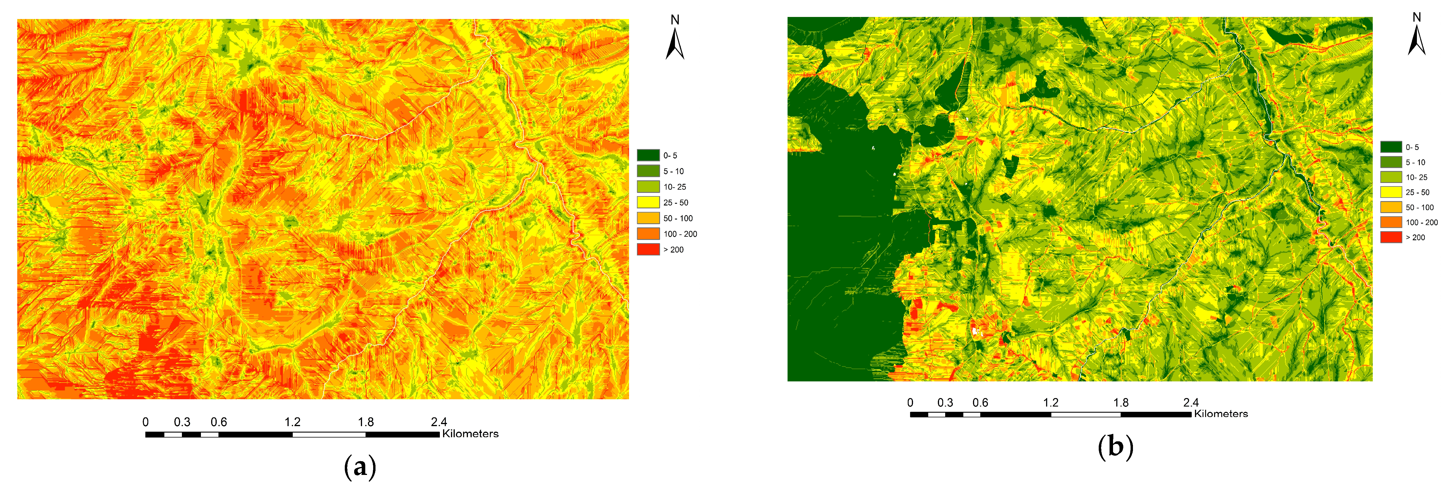
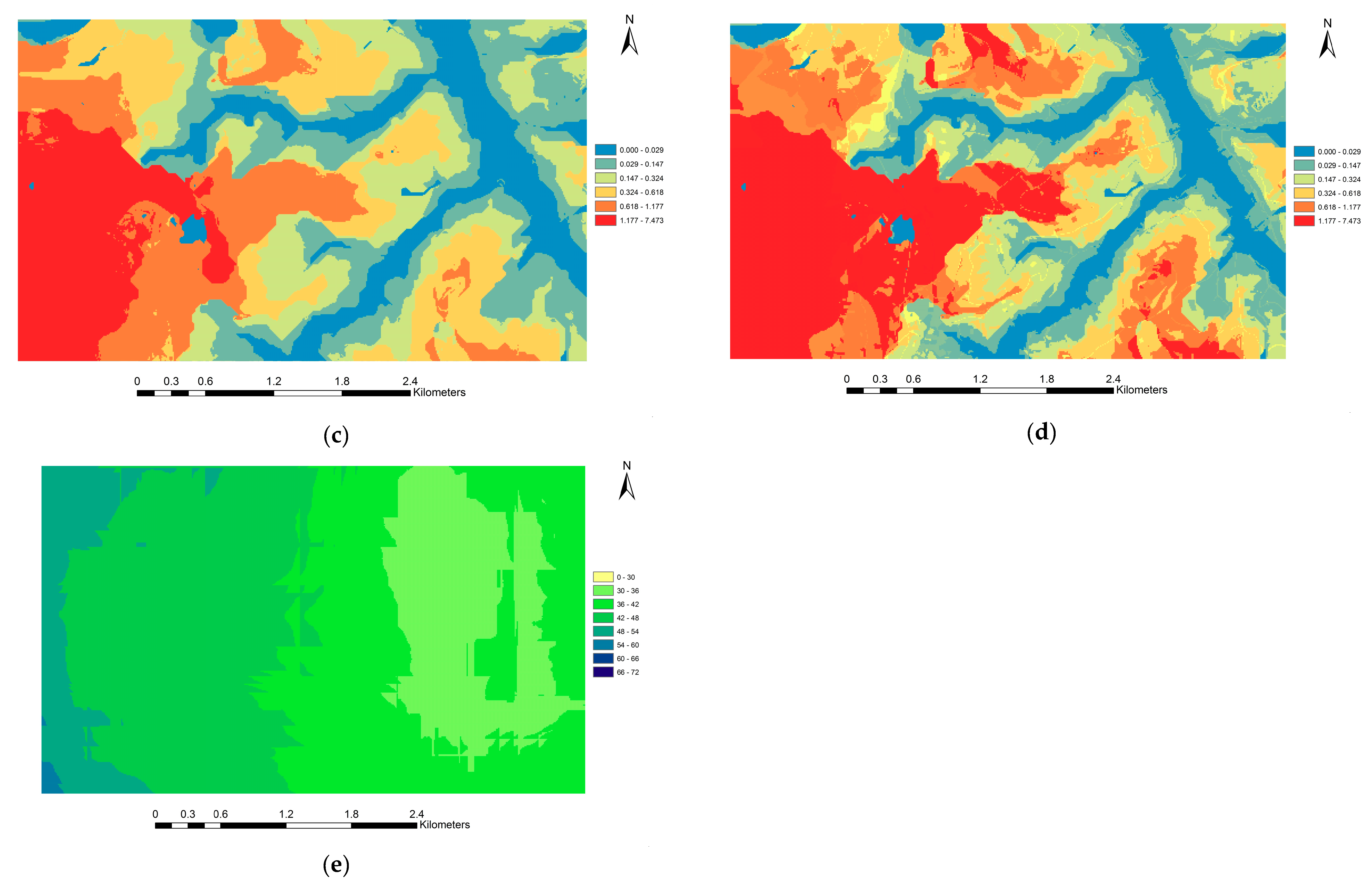
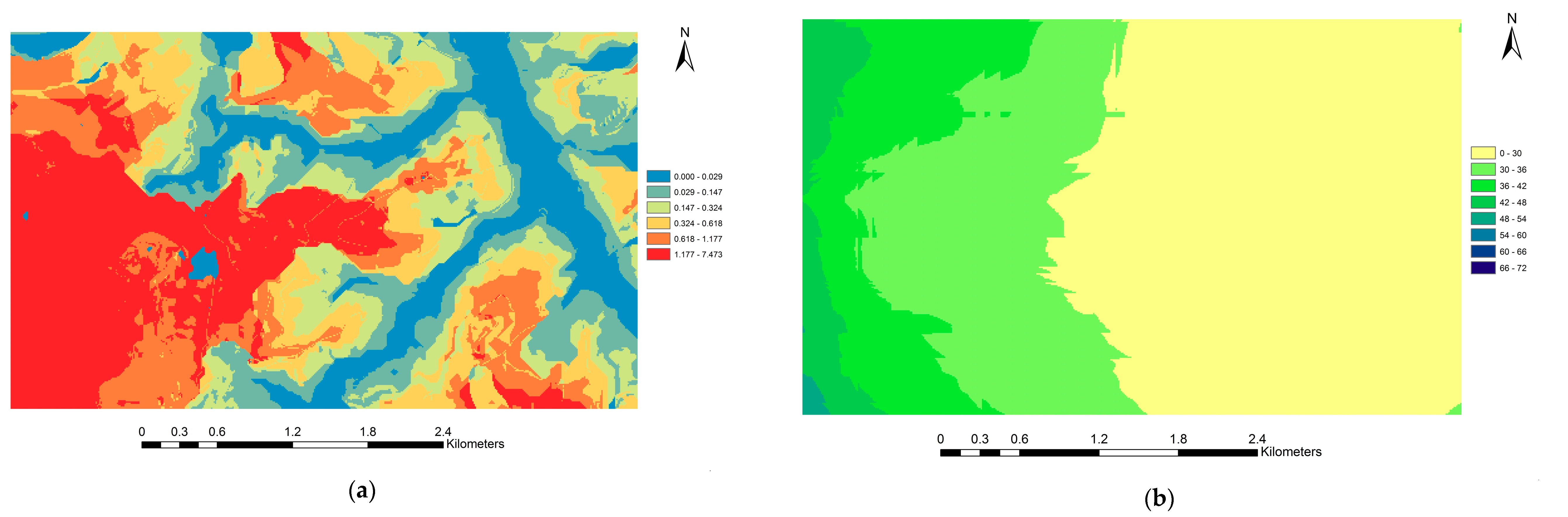
It can be observed (

Table 2. Agri-environmental indicators for each olive grove type in HSL (high slope landscape, Sierra Mágina) corresponding to the current situation (0). All values are means ± SD. N = total number of estates devoted to olive cultivation; ErPot = Potential erosion; ErI = Erosion indicator; DPoPot = Potential diffuse pollution; Dslpe. = Downslope area potentially affected by diffuse pollution; N.Tr. = Number of agro-chemical treatments; DPoI = Diffuse pollution indicator; DvI = Diversity indicator.

HSL-0
AEMO Code*	N	ErPot (x ± SD)	ErI (x ± SD)	DPoPot (x ± SD)	Dslp. Area (ha)	N. Tr.	DPoI (x ± SD)	DvI (x ± SD)
OTNMS	477	142.43 ± 82.11	36.14 ± 22.49	0.453 ± 0.359	122.06 ± 102.01	2	0.907 ± 0.717	43.45 ± 3.92
OTMS	390	55.29 ± 23.92	14.2 ± 6.51	0.42 ± 0.397	105.03 ± 92.69	3	1.259 ± 1.191	42.07 ± 4.58
OIS	20	51.28 ± 24.12	13.02 ± 5.63	0.509 ± 0.469	121.18 ± 109.54	4	2.035 ± 1.876	41.67 ± 3.13
OISP	30	190.11 ± 126.17	48.03 ± 32.71	0.688 ± 0.413	189.06 ± 117.00	4	2.751 ± 1.65	43.58 ± 3.06
OTNMR	785	111.73 ± 42.79	28.46 ± 11.96	0.119 ± 0.151	26.51 ± 33.18	2	0.238 ± 0.301	39.83 ± 3.37
OTMR	1041	63.47 ± 25.35	17.44 ± 7.78	0.149 ± 0.199	36.53 ± 45.94	3	0.448 ± 0.596	37.52 ± 3.12
OIR	63	64.78 ± 27.81	19.39 ± 9.82	0.134 ± 0.198	32.16 ± 46.03	4	0.535 ± 0.793	37.61 ± 3.08
OIRP	59	133.33 ± 59.61	35.36 ± 16.64	0.097 ± 0.145	21.28 ± 31.92	4	0.388 ± 0.58	41.12 ± 2.47
Total	2865	91.44 ± 57.96	23.83 ± 15.44	0.235 ± 0.300	59.41 ± 77.12	2.62 ± 0.6	0.613 ± 0.828	39.93 ± 4.20

AEMO code*: OTNMS: Sloped traditional rain-fed olive groves; OTMS: Traditional rain-fed olive groves; OIS: Intensive rain-fed olive groves; OISP: Sloped intensive rain-fed olive groves; OTNMR: Sloped traditional irrigated olive groves; OTMR: Traditional irrigated olive groves; OIR: Intensive irrigated olive groves; OIRP: Sloped intensive irrigated olive groves; OES: Rain-fed ecological olive grove; OER: Irrigated ecological olive grove.

) that HSL, consistently with its stronger altitudinal gradient, presented the highest values of potential erosion (91.44 t·ha⁻¹·yr⁻¹, Figure 2a), and of estimated erosion (23.83 t·ha⁻¹·yr⁻¹, Figure 2b). In addition, it showed an intermediate to high potential for diffuse pollution risk (DPoPot = 0.235, Figure 2c), and a low spatial diversity (DvI = 39.93%, Figure 2e). The high slope characteristic could be observed also from the individual olive grove type perspective, with high slope olive grove types showing the highest values for both potential and estimated erosion. Potential diffuse pollution showed a different trend, with higher values for rain-fed olive groves (0.42–0.688) and lower for those irrigated (0.097–0.149). This trend was still retained when the number of agro-chemical treatments was taken into account (Figure 2d), as the dominant parameter for DPoI is downslope area potentially affected by runoff pollution, and that was always higher for rain-fed olive groves (105.03–189.06 ha) than for irrigated (21.28–36.53 ha).

The values obtained for MSL (

Table 3. Agri-environmental indicators for each olive grove type in MSL (medium slope landscape, Bajo Aragón) corresponding to the current situation (0). All values are means ± SD. N = total number of estates devoted to olive cultivation; ErPot = Potential erosion; ErI = Erosion indicator; DPoPot = Potential diffuse pollution; Dslpe. = Downslope area potentially affected by diffuse pollution; N.Tr. = Number of agro-chemical treatments; DPoI = Diffuse pollution indicator; DvI = Diversity indicator.

MSL-0
AEMO Code*	N	ErPot (x ± SD)	ErI (x ± SD)	DPoPot (x ± SD)	Dslp. Area (ha)	N. Tr.	DPoI (x ± SD)	DvI (x ± SD)
OTNMS	3	159.67 ± 26.38	44.88 ± 25.72	0.060 ± 0.084	13.99 ± 19.74	2	0.119 ± 0.168	58.95 ± 1.99
OTMS	432	53.48 ± 24.49	10.58 ± 7.22	0.073 ± 0.071	19.06 ± 18.36	3	0.219 ± 0.212	59.07 ± 2.85
OTMR	1	39.7	8.16	0.064	16.81	3	0.193	60.74
Total	436	54.18 ± 25.99	10.81 ± 7.92	0.073 ± 0.071	19.02 ± 18.33	2.99 ± 0.08	0.218 ± 0.212	59.07 ± 2.84

AEMO code*: OTNMS: Sloped traditional rain-fed olive groves; OTMS: Traditional rain-fed olive groves; OIS: Intensive rain-fed olive groves; OISP: Sloped intensive rain-fed olive groves; OTNMR: Sloped traditional irrigated olive groves; OTMR: Traditional irrigated olive groves; OIR: Intensive irrigated olive groves; OIRP: Sloped intensive irrigated olive groves; OES: Rain-fed ecological olive grove; OER: Irrigated ecological olive grove.

), showed its intermediate character for potential and estimated erosion (ErPot = 54.18 t·ha⁻¹·yr⁻¹, ErI = 10.81 t·ha⁻¹·yr⁻¹ respectively), and also for spatial diversity (DvI = 59.07 %). In contrast, MSL attained the lowest values for the risk of potential diffused pollution (DPoPot = 0.073), following the trend of the downslope area potentially affected by runoff pollution (range 13.99–19.06 ha). In this landscape high slope olive groves are scarce, but even so the expected sequence regarding potential and estimated erosion was still observable. Spatial diversity was very similar among olive grove types.

LSL had the lowest values of potential and estimated erosion (29.51 t·ha⁻¹·yr⁻¹ and 6.65 t·ha⁻¹·yr⁻¹, respectively; see

Table 4. Agri-environmental indicators for each olive grove type in LSL (low slope landscape, Bajo Aragón) corresponding to the current situation (0). All values are means ± SD. N = total number of estates devoted to olive cultivation; ErPot = Potential erosion; ErI = Erosion indicator; DPoPot = Potential diffuse pollution; Dslpe. = Downslope area potentially affected by diffuse pollution; N.Tr. = Number of agro-chemical treatments; DPoI = Diffuse pollution indicator; DvI = Diversity indicator.

LSL-0
AEMO Code*	N	ErPot (x ± SD)	ErI (x ± SD)	DPoPot (x ± SD)	Dslp. Area (ha)	N. Tr.	DPoI (x ± SD)	DvI (x ± SD)
OTMS	305	29.48 ± 12.65	6.64 ± 2.4	0.42 ± 0.367	226.98 ± 193.22	3	1.261 ± 1.102	64.03 ± 2.86
OTMR	6	31.08 ± 8.34	7.05 ± 1.29	0.211 ± 0.343	70.49 ± 113.04	3	0.634 ± 1.028	67.29 ± 2.66
Total	311	29.51 ± 12.57	6.65 ± 2.39	0.416 ± 0.367	222.69 ± 193.08	3.00 ± 0.00	1.249 ± 1.102	64.09 ± 2.88

AEMO code*: OTNMS: Sloped traditional rain-fed olive groves; OTMS: Traditional rain-fed olive groves; OIS: Intensive rain-fed olive groves; OISP: Sloped intensive rain-fed olive groves; OTNMR: Sloped traditional irrigated olive groves; OTMR: Traditional irrigated olive groves; OIR: Intensive irrigated olive groves; OIRP: Sloped intensive irrigated olive groves; OES: Rain-fed ecological olive grove; OER: Irrigated ecological olive grove.

). In addition, it showed the highest values for diffuse pollution risk (DPoPot = 0.416, DPoI = 1.249), and spatial diversity (DvI = 64.09%). In this landscape only traditional olive groves were present (both rain-fed and irrigated, OTMS and OTMR), without high slope or intensive types. Consequently, potential and estimated erosion were the lowest, with only slight differences between olive groves (highly overlapping intervals). In contrast, potential and estimated diffuse pollution risks were the highest of all study areas (again with highly overlapping intervals between types). Values for downslope area potentially affected by runoff pollution followed the same trend, with similar high variance (226.98 ± 193.22 ha for OTMS; 70.49 ± 113.04 ha for OTMR). Spatial diversity attained also the highest values of all, without great differences between olive grove types.

3.2. Management Scenarios

The changes assumed by the ecological scenario (high slope to ecological production), mean a clear decrease in agro-chemical treatments (no use for those olive grove types), and both a reduction in RUSLE factor C (by keeping herbaceous natural cover) and a potentially more intricate landscape. This is attained by the replacement of up to four olive grove types by four new ones in which the herbaceous natural cover somehow implies the introduction of natural elements into agricultural ground. This mixture has a positive effect on biodiversity, and changes the spatial configuration of land uses.

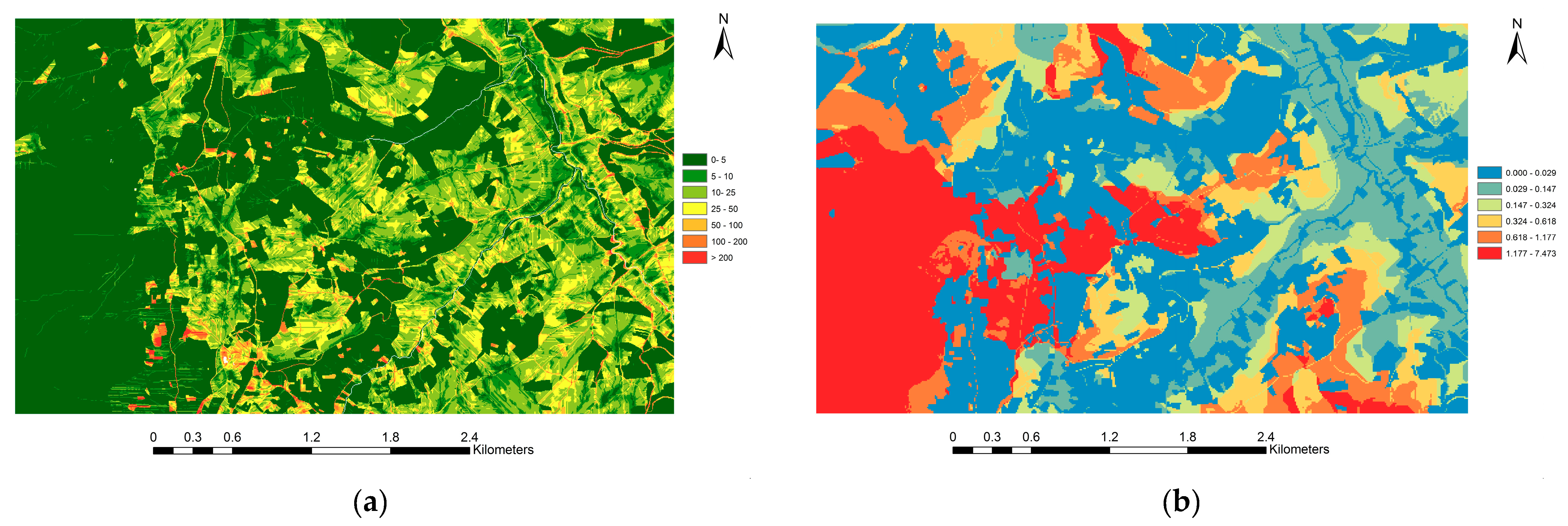
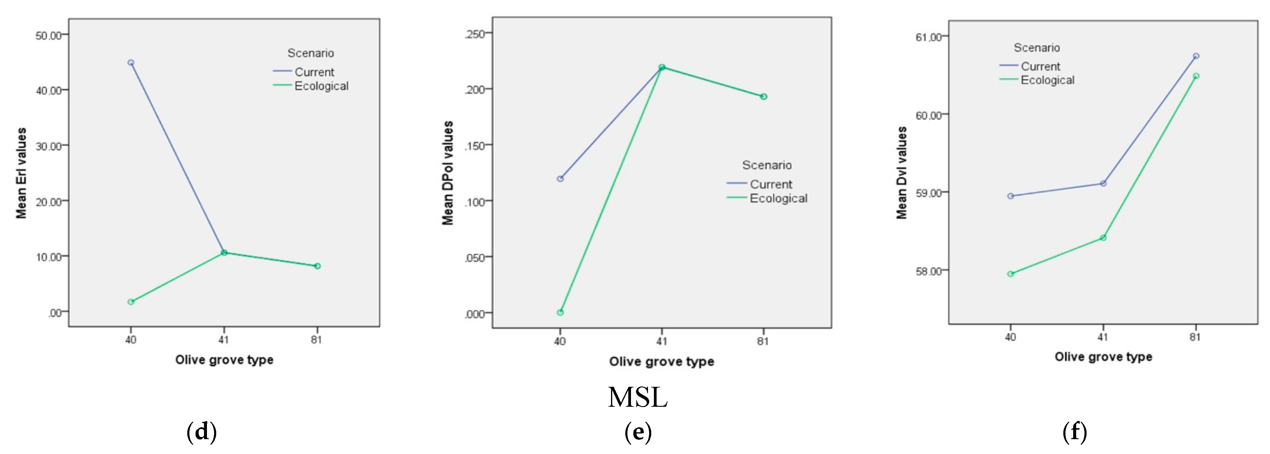
An ecological scenario that involved applying these ‘greener’ measures to high slope olive groves would affect our study areas differently: HSL would be the most sensitive landscape (35% of its area is devoted to the target management type), and Bajo Aragón the least affected (MSL had only 0.06%, and LSL 0%). According to these expectations,

Table 5. Agri-environmental indicators for each olive grove type in HSL (high slope landscape, Sierra Mágina) corresponding to the ecological scenario (1). All values are means ± SD. N = total number of estates devoted to olive cultivation; ErPot = Potential erosion; ErI = Erosion indicator; DPoPot = Potential diffuse pollution; Dslpe. = Downslope area potentially affected by diffuse pollution; N.Tr. = Number of agro-chemical treatments; DPoI = Diffuse pollution indicator; DvI = Diversity indicator.

HSL-1
AEMO Code* (Initial)	N	ErPot (x ± SD)	DPoPot (x ± SD)	Dslp. Area (ha)	AEMO Code* (Final)	ErI (x ± SD)	N. Tr.	DPoI (x ± SD)	DvI (x ± SD)
OTNMS	477	142.43 ± 82.11	0.453 ± 0.359	122.06 ± 102.01	OES	2.06 ± 1.25	0	0.00 ± 0.00	54.66 ± 2.81
OTMS	390	55.29 ± 23.92	0.42 ± 0.397	105.03 ± 92.69	OTMS	14.2 ± 6.51	3	1.259 ± 1.191	54.3 ± 3.44
OIS	20	51.28 ± 24.12	0.509 ± 0.469	121.18 ± 109.54	OIS	13.02 ± 5.63	4	2.035 ± 1.876	53.3 ± 2.72
OISP	30	190.11 ± 126.17	0.688 ± 0.413	189.06 ± 117	OEISP	2.81 ± 1.88	0	0.00 ± 0.00	54.45 ± 1.95
OTNMR	785	111.73 ± 42.79	0.119 ± 0.151	26.51 ± 33.18	OER	1.59 ± 0.66	0	0.00 ± 0.00	52.73 ± 2.76
OTMR	1,041	63.47 ± 25.35	0.149 ± 0.199	36.53 ± 45.94	OTMR	17.44 ± 7.78	3	0.448 ± 0.596	51.17 ± 2.67
OIR	63	64.78 ± 27.81	0.134 ± 0.198	32.16 ± 46.03	OIR	19.39 ± 9.82	4	0.535 ± 0.793	51.33 ± 2.62
OIRP	59	133.33 ± 59.61	0.097 ± 0.145	21.28 ± 31.92	OEIRP	1.93 ± 0.9	0	0.00 ± 0.00	53.22 ± 2.04
Total	2,865	91.44 ± 57.96	0.235 ± 0.300	59.41 ± 77.12	Total	9.64 ± 9.31	1.61 ± 1.53	0.360 ± 0.743	52.7 ± 3.13

AEMO code*: OTNMS: Sloped traditional rain-fed olive groves; OTMS: Traditional rain-fed olive groves; OIS: Intensive rain-fed olive groves; OISP: Sloped intensive rain-fed olive groves; OTNMR: Sloped traditional irrigated olive groves; OTMR: Traditional irrigated olive groves; OIR: Intensive irrigated olive groves; OIRP: Sloped intensive irrigated olive groves; OES: Sloped rain-fed ecological olive groves; OEISP: Sloped intensive ecological rain-fed olive groves; OER: Sloped irrigated ecological olive groves; OEIRP: Sloped intensive irrigated ecological olive groves.

shows a highly reduced erosion for HSL (global ErI diminished even below MSL, 9.64 vs. 10.62 t·ha⁻¹·yr⁻¹, respectively; see Figure 3a), a reduction of almost 50% in global DPoI for HSL (Figure 3b), and an increase in global DvI almost to Bajo Aragón levels (52.7%, Figure 3c). Changes in Bajo Aragón were small for MSL, and non-existent for LSL (

Table 6. Agri-environmental indicators for each olive grove type in MSL (medium slope landscape, Bajo Aragón) corresponding to the ecological scenario (1). All values are means ± SD. N = total number of estates devoted to olive cultivation; ErPot = Potential erosion; ErI = Erosion indicator; DPoPot = Potential diffuse pollution; Dslpe. = Downslope area potentially affected by diffuse pollution; N.Tr. = Number of agro-chemical treatments; DPoI = Diffuse pollution indicator; DvI = Diversity indicator.

MSL-1
AEMO Code* (Initial)	N	ErPot (x ± SD)	DPoPot (x ± SD)	Dslp. Area(ha)	AEMO Code* (Final)	ErI (x ± SD)	N. Tr.	DPoI (x ± SD)	DvI (x ± SD)
OTNMS	3	159.67 ± 26.38	0.060 ± 0.084	13.99 ± 19.74	OES	1.68 ± 0.96	0	0.00 ± 0.00	57.95 ± 1.76
OTMS	432	53.48 ± 24.49	0.073 ± 0.071	19.06 ± 18.36	OTMS	10.58 ± 7.22	3	0.219 ± 0.212	58.35 ± 3.03
OTMR	1	39.7	0.064	16.81	OTMR	8.16	3	0.193	60.45
Total	436	54.18 ± 25.99	0.073 ± 0.071	19.02 ± 18.33	Total	10.52 ± 7.23	2.98 ± 0.25	0.218 ± 0.212	58.35 ± 3.02

AEMO code*: OTNMS: Sloped traditional rain-fed olive groves; OTMS: Traditional rain-fed olive groves; OIS: Intensive rain-fed olive groves; OISP: Sloped intensive rain-fed olive groves; OTNMR: Sloped traditional irrigated olive groves; OTMR: Traditional irrigated olive groves; OIR: Intensive irrigated olive groves; OIRP: Sloped intensive irrigated olive groves; OES: Rain-fed ecological olive grove.

and

Table 7. Agri-environmental indicators for each olive grove type in LSL (low slope landscape, Bajo Aragón) corresponding to the ecological scenario (1). All values are means ± SD. N = total number of estates devoted to olive cultivation; ErPot = Potential erosion; ErI = Erosion indicator; DPoPot = Potential diffuse pollution; Dslpe. = Downslope area potentially affected by diffuse pollution; N.Tr. = Number of agro-chemical treatments; DPoI = Diffuse pollution indicator; DvI = Diversity indicator.

LSL-1
AEMO Code* (Initial)	N	ErPot (x ± SD)	DPoPot (x ± SD)	Dslp. Area (ha)	AEMO Code* (Final)	ErI (x ± SD)	N. Tr.	DPoI (x ± SD)	DvI (x ± SD)
OTMS	305	29.48 ± 12.65	0.42 ± 0.367	226.98 ± 193.22	OTMS	6.64 ± 2.4	3	1.261 ± 1.102	64.03 ± 2.86
OTMR	6	31.08 ± 8.34	0.211 ± 0.343	70.49 ± 113.04	OTMR	7.05 ± 1.29	3	0.634 ± 1.028	67.29 ± 2.66
Total	311	29.51 ± 12.57	0.416 ± 0.367	222.69 ± 193.08	Total	6.65 ± 2.39	3.00 ± 0.00	1.249 ± 1.102	64.09 ± 2.88

AEMO code*: OTNMS: Sloped traditional rain-fed olive groves; OTMS: Traditional rain-fed olive groves; OIS: Intensive rain-fed olive groves; OISP: Sloped intensive rain-fed olive groves; OTNMR: Sloped traditional irrigated olive groves; OTMR: Traditional irrigated olive groves; OIR: Intensive irrigated olive groves; OIRP: Sloped intensive irrigated olive groves.

). The repeated measures ANOVAs confirmed that the changes registered by the three indicators were statistically significant. For HSL, the landscape most affected by the ecological scenario, there were overall differences between current and ecological values for all three indicators (between-subjects factor p < 0.001), and for the overall set of olive grove types (inter-subjects factor, p < 0.001). Furthermore, in spite of the fact that indicator values were only different for the affected olive grove types (4 out of 8), the interaction between scenario and olive grove type was also highly significant for all three indicators (p < 0.001). Figure 4a–c show the interaction graphs, from which it is to be noted the different behavior of DvI; whereas ErI and DPoI only change for those olive grove types targeted by the ecological scenario, DvI changes remarkably for all olive grove types. Results for MSL, although affected by the low abundance of farms with the target olive grove types, also showed significant effects of scenario (p < 0.001), management type (p < 0.001) and their interaction (p < 0.001) for ErI and DPoI. The exception was the DvI, for which the interaction was not significant (p = 0.087). Figure 4d–f show the interaction graphs for the three indicators. For the LSL landscape, as there were no target olive grove types, indicator values did not change for the ecological scenario.

The changes assumed by the productive scenario (rain-fed to irrigated, and traditional to intensive if currently irrigated) mean a clear increase in agro-chemical treatments with intensification, and both a landscape simplification, and different spatial configuration of land uses. There is a landscape simplification because rain-fed olive grove types disappear (potentially 4 out of 8), but no new intensive olive grove type is gained to compensate for the loss, so the overall result is the loss of 1–4 olive grove types in all study areas. Therefore all study areas are expected to respond to the changes involved, although again in a decreasing way due to overall area occupied by olive groves (highest in HSL) and proportion of irrigated relative to rain-fed types (lowest in Bajo Aragón).

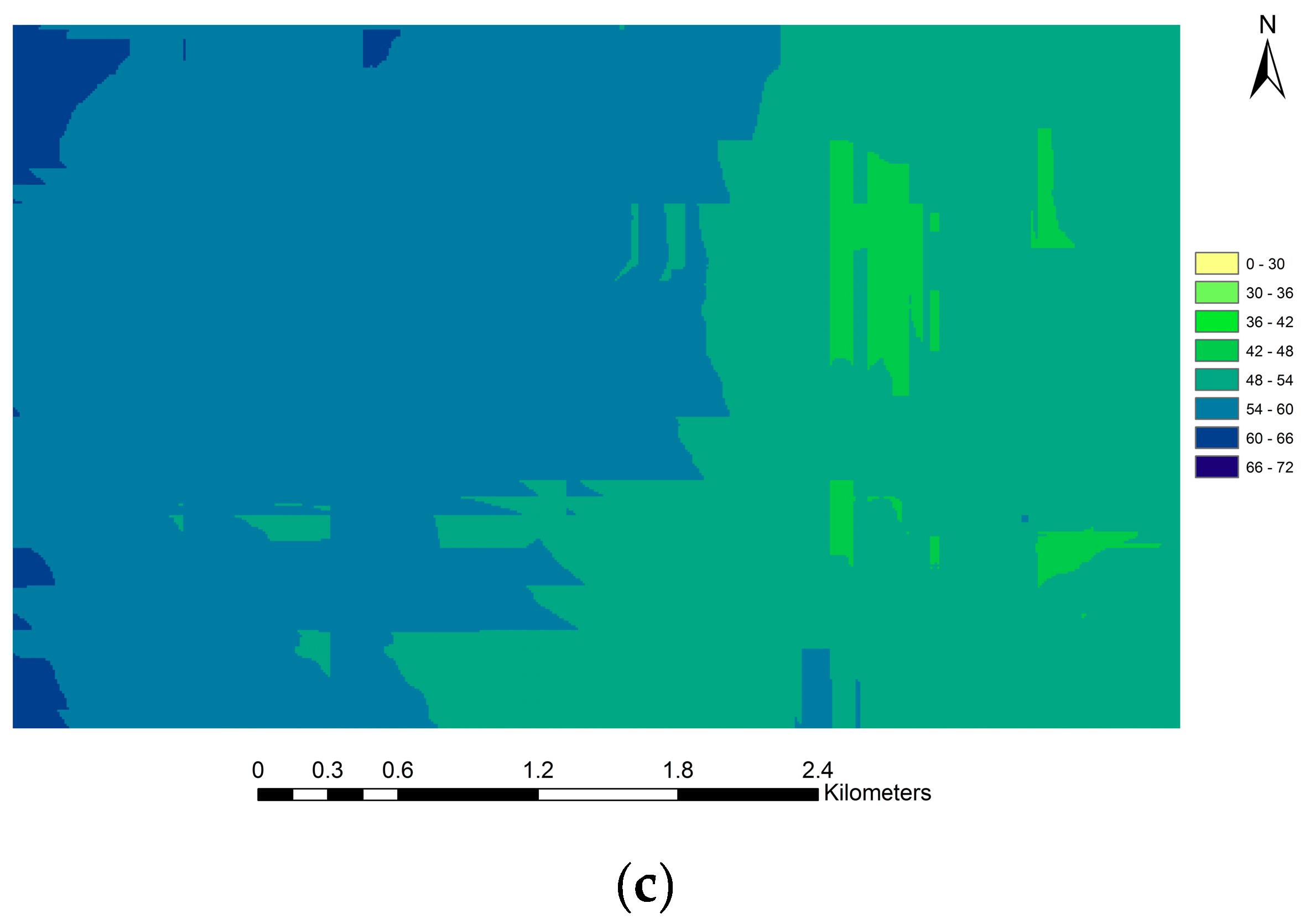
In this scenario (see

Table 8. Agri-environmental indicators for each olive grove type in HSL (high slope landscape, Sierra Mágina) corresponding to the productive scenario (2). All values are means ± SD. N = total number of estates devoted to olive cultivation; ErPot = Potential erosion; ErI = Erosion indicator; DPoPot = Potential diffuse pollution; Dslpe. = Downslope area potentially affected by diffuse pollution; N.Tr. = Number of agro-chemical treatments; DPoI = Diffuse pollution indicator; DvI = Diversity indicator.

HSL-2
AEMO Code* (Initial)	N	ErPot (x ± SD)	DPoPot (x ± SD)	Dslp. Area (ha)	AEMO Code* (Final)	ErI (x ± SD)	N. Tr.	DPoI (x ± SD)	DvI (x ± SD)
OTNMS	477	142.43 ± 82.11	0.453 ± 0.359	122.06 ± 102.01	OTNMR	36.14 ± 22.49	2	0.907 ± 0.717	32.25 ± 5.17
OTMS	390	55.29 ± 23.92	0.42 ± 0.397	105.03 ± 92.69	OTMR	14.2 ± 6.51	3	1.259 ± 1.191	30.02 ± 5.68
OIS	20	51.28 ± 24.12	0.509 ± 0.469	121.18 ± 109.54	OIR	13.02 ± 5.63	4	2.035 ± 1.876	29.97 ± 3.31
OISP	30	190.11 ± 126.17	0.688 ± 0.413	189.06 ± 117	OIRP	48.03 ± 32.71	4	2.751 ± 1.650	32.44 ± 4.26
OTNMR	785	111.73 ± 42.79	0.119 ± 0.151	26.51 ± 33.18	OIRP	28.46 ± 11.96	4	0.477 ± 0.602	27.13 ± 4.23
OTMR	1041	63.47 ± 25.35	0.149 ± 0.199	36.53 ± 45.94	OIR	17.44 ± 7.78	4	0.598 ± 0.794	24.37 ± 3.56
OIR	63	64.78 ± 27.81	0.134 ± 0.198	32.16 ± 46.03	OIR	19.39 ± 9.82	4	0.535 ± 0.793	24.31 ± 3.4
OIRP	59	133.33 ± 59.61	0.097 ± 0.145	21.28 ± 31.92	OIRP	35.36 ± 16.64	4	0.388 ± 0.58	29.02 ± 3.46
Total	2865	91.44 ± 57.96	0.235 ± 0.300	59.41 ± 77.12	Total	23.83 ± 15.44	3.53 ± 0.76	0.733 ± 0.896	27.42 ± 5.28

AEMO code*: OTNMS: Sloped traditional rain-fed olive groves; OTMS: Traditional rain-fed olive groves; OIS: Intensive rain-fed olive groves; OISP: Sloped intensive rain-fed olive groves; OTNMR: Sloped traditional irrigated olive groves; OTMR: Traditional irrigated olive groves; OIR: Intensive irrigated olive groves; OIRP: Sloped intensive irrigated olive groves; OES: Rain-fed ecological olive grove; OER: Irrigated ecological olive grove.

), there was no change in ErI for the three landscapes, as there was no change of plant covers relative to the current situation. In contrast, DPoI and DvI did reflect the management change mainly in HSL, increasing in the first case (0.630 to 0.733, Figure 5a) due to intensification of irrigated olive groves, and decreasing in the second (39.93% to 27.42%, Figure 5b), due to the loss of the rain-fed type and the related changes in spatial configuration. MSL and LSL also showed differences, but very slight due to the reduced areas involved (see

Table 9. Agri-environmental indicators for each olive grove type in MSL (medium slope landscape, Bajo Aragón) corresponding to the productive scenario (2). All values are means ± SD. N = total number of estates devoted to olive cultivation; ErPot = Potential erosion; ErI = Erosion indicator; DPoPot = Potential diffuse pollution; Dslpe. = Downslope area potentially affected by diffuse pollution; N.Tr. = Number of agro-chemical treatments; DPoI = Diffuse pollution indicator; DvI = Diversity indicator.

MSL-2
AEMO Code* (Initial)	N	ErPot (x ± SD)	DPoPot (x ± SD)	Dslp. Area (ha)	AEMO Code* (Final)	ErI (x ± SD)	N. Tr.	DPoI (x ± SD)	DvI (x ± SD)
OTNMS	3	159.67 ± 26.38	0.060 ± 0.084	13.99 ± 19.74	OTNMR	44.88 ± 25.72	2	0.119 ± 0.168	59.15 ± 1.85
OTMS	432	53.48 ± 24.49	0.073 ± 0.071	19.06 ± 18.36	OTMR	10.58 ± 7.22	3	0.219 ± 0.212	59.17 ± 2.85
OTMR	1	39.7	0.064	16.81	OIR	8.16	4	0.256	60.4768
Total	436	54.18 ± 25.99	0.073 ± 0.071	19.02 ± 18.33	Total	10.81 ± 7.92	3.00 ± 0.1	0.219 ± 0.211	59.17 ± 2.85

AEMO code*: OTNMS: Sloped traditional rain-fed olive groves; OTMS: Traditional rain-fed olive groves; OIS: Intensive rain-fed olive groves; OISP: Sloped intensive rain-fed olive groves; OTNMR: Sloped traditional irrigated olive groves; OTMR: Traditional irrigated olive groves; OIR: Intensive irrigated olive groves; OIRP: Sloped intensive irrigated olive groves; OES: Rain-fed ecological olive grove; OER: Irrigated ecological olive grove.

and

Table 10. Agri-environmental indicators for each olive grove type in LSL (low slope landscape, Bajo Aragón) corresponding to the productive scenario (2). All values are means ± SD. N = total number of estates devoted to olive cultivation; ErPot = Potential erosion; ErI = Erosion indicator; DPoPot = Potential diffuse pollution; Dslpe. = Downslope area potentially affected by diffuse pollution; N.Tr. = Number of agro-chemical treatments; DPoI = Diffuse pollution indicator; DvI = Diversity indicator.

LSL-2
AEMO Code* (Initial)	N	ErPot (x ± SD)	DPoPot (x ± SD)	Dslp. Area (ha)	AEMO Code* (Final)	ErI (x ± SD)	N. Tr.	DPoI (x ± SD)	DvI (x ± SD)
OTMS	305	29.48 ± 12.65	0.42 ± 0.367	226.98 ± 193.22	OTMR	6.64 ± 2.4	3	1.261 ± 1.102	64.2 ± 3.47
OTMR	6	31.08 ± 8.34	0.211 ± 0.343	70.49 ± 113.04	OIR	7.05 ± 1.29	4	0.845 ± 1.37	63.3 ± 3.03
Total	311	29.51 ± 12.57	0.416 ± 0.367	222.69 ± 193.08	Total	6.65 ± 2.39	3.02 ± 0.14	1.253 ± 1.106	64.19 ± 3.46

AEMO code*: OTNMS: Sloped traditional rain-fed olive groves; OTMS: Traditional rain-fed olive groves; OIS: Intensive rain-fed olive groves; OISP: Sloped intensive rain-fed olive groves; OTNMR: Sloped traditional irrigated olive groves; OTMR: Traditional irrigated olive groves; OIR: Intensive irrigated olive groves; OIRP: Sloped intensive irrigated olive groves; OES: Rain-fed ecological olive grove; OER: Irrigated ecological olive grove.

).

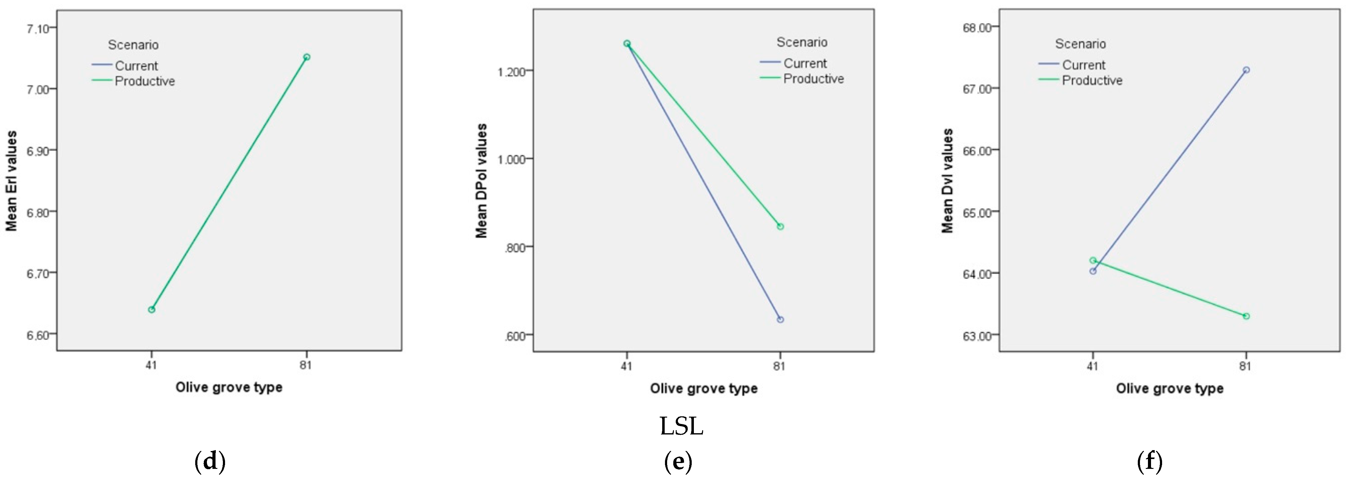
For HSL, the repeated measures ANOVAs showed that there were overall differences between current and productive values for DPoI and DvI indicators (between-subjects factor p < 0.001), and for the overall set of olive grove types (inter-subjects factor, p < 0.001). As there was no change in RUSLE factor C, ErI did not change. Consequently, the interaction between scenario and management type was only significant for DPoI and DvI (p < 0.001). Figure 6a–c show the interaction graphs, from which it is again to be noted the different behavior of DvI; whereas DPoI only changed for the irrigated olive grove types, (2 out of 8), DvI changed remarkably for all olive grove types. In contrast, due to the high predominance of only one olive grove type, ANOVA results for MSL only showed significant effects of scenario (p < 0.001), management type (p < 0.001) and their interaction (p < 0.001) for DPoI. For LSL landscape, indicator values responded significantly to scenario (p < 0.001), management type (p < 0.001) and to their interaction (p < 0.001) for DPoI and DvI. Again, as Figure 6f shows, the response of DvI was remarkable in magnitude.

4. Discussion

Our results showed that agri-environmental externalities studied can be assessed with the indicators proposed, because they are able to distinguish among different environmental and management situations, and respond significantly to their changes in a way directly relatable to the mechanisms underlying each indicator. Several studies [46,47] agree on the importance of improving indicators to quantify these environmental externalities, to be used as a guiding tool both at farm management and environmental policy design levels. In Spain, traditional olive groves are usually located in semi-arid and arid climatic conditions, associated with degraded soils and complex geology and relief [20], with agricultural diffuse pollution being an especially troubling issue [21,48].

The environmental indicators proposed were able to identify the different landscapes by their mean values of potential erosion (HSL > MSL > LSL) and diffuse pollution (LSL > HSL > MSL). Slope was the key parameter behind potential erosion, and total potentially affected downslope area for diffuse pollution. Higher slope values are associated with higher values of potential erosion, both considering landscapes separately and averaging across landscapes (high slope olive groves: 125.33 ± 65.09; low slope olive groves: 55.39 ± 26.13 t·ha⁻¹·yr⁻¹). Downslope area is not that intuitive, as size and shape of micro-watersheds depend on current geomorphologic and topographical characteristics, which in turn are a function of geology, slope and environmental history (including past land uses that could have conditioned present erosion land forms).

An essential part of the methodology proposed is the substitution of non-available data (mainly measurements at farm level) with available surrogates that could constitute accurate enough approximations to be used in environmental externalities assessment. In the present study this is represented mainly by the use of geologic maps to derive edaphic parameters. The available data we found was only comparable with the erosion indicator (ErI), and it showed that our results were completely in the range of those obtained by other authors (e.g., [49,50,51]). Specifically, Vanwalleghem and coworkers [52] measured an average soil erosion rate between 29 and 47 t·ha⁻¹·yr⁻¹, for three medium-high slope sites in southern Spain, over a 250-year period. For a slope range of 12.75–36.46%, we obtained a comparable range of 19.39–48.03 t·ha⁻¹·yr⁻¹. Similarly, studying low slope olive groves in Córdoba (southern Spain), Gomez and coworkers [50] estimated an average of 12.47 t·ha⁻¹·yr⁻¹ for conventional rain-fed olive crops, and 1.95 t·ha⁻¹·yr⁻¹ for the complete herbaceous cover alternative. As the rest of the edaphic parameters are based mainly in the same parent material characteristics as factor K, the procedure can be considered valid for the purpose of agro-environmental externalities assessment.

The agri-environmental indicators also showed a good response to the management changes introduced by the different scenarios proposed. In general, this response implied a change in indicator values of similar magnitude to that of the corresponding driving variable. Thus, for example, a reduction of 96% in factor C for the ecological scenario gave a reduction of 93.94–96.25% in estimated erosion, or an increase of 33.33% in the number of agro-chemical treatments gave a similar increase in the diffuse pollution indicator.

In contrast, the spatial diversity indicator showed a different behavior regarding response level: instead of being linear, it was several times greater or lower than the change in its driving variable (in this case, the number of land-use types), depending on landscape. For HSL, an increment or decrement of 8.33% in the number of land uses brought about a change of the same sign ranging from 25.89–36.83% in spatial diversity, for all olive grove types. Conversely, in MSL an increase of 7.14% gave a decrease of 1.2%, and a similar decrease produced an increase of 0.2%. For LSL, the same decrease induced both a positive (0.27%) and a negative response (−5.91%) depending on olive grove type considered. This was further confirmed by the statistical results: although scenario changes involved only a part of the potential olive grove types, the response given by the DvI affected all of them (Figure 4c and Figure 6c,f). Only in those cases where the number of the target olive grove types was insufficient for statistical detection (MSL), scenario and management interaction was not significant. Therefore, the spatial diversity indicator did respond to the changes in its driving variable, and this response could be said to be non-linear. This fact reveals the importance of spatial configuration for landscape function: the gain or loss of a land-use has different consequences depending on where that change takes place (i.e., the landscape context).

Landscape configuration can affect the processes involved in the agri-environmental externalities considered, buffering or amplifying the management effects on agro-ecosystem function. For example, different plant covers interact differently with pollutants and sediments in runoff water, whose flow they can also modify, thus altering the final outcome of diffuse pollution and erosion [53,54]. The spatial configuration of land-covers can affect biodiversity, modifying individual patch size and connectivity with similar patches [55], acting as ecological barriers or corridors for species dispersal [56], thus potentially increasing or decreasing α and β diversity [57], and favoring or deterring phenomena like plague susceptibility [58]. Therefore, to better address the question of biodiversity at landscape scale, it is clear that some empirical data about the species composition of each land-cover would improve the performance of any landscape metric used as an indicator of agri-environmental impact on biodiversity.

5. Conclusions

Indicators play an essential role in objectively assessing actions and processes involved in the ecological, economic, and social aspects of sustainable agriculture. Available indicators allow the farmers to contrast their farming practices related to nutrient balances, energy efficiency or productivity [59]. However, regarding some of the agri-environmental externalities examined in this paper (namely diffuse pollution and biodiversity), work is still needed to improve existing indicators if they are intended to be used a guide in land planning and socio-ecological landscapes management.

Our results showed that the indicators proposed can be used to assess these agri-environmental externalities, because they are able to distinguish among different environmental and management situations, and show a good response to their changes in the different scenarios proposed, in a way directly relatable to the mechanisms underlying each indicator. In addition, our findings highlight the importance of landscape structure (composition and configuration), that could even play an important role in the behavior of the environmental externalities. This suggests the necessity of incorporating some kind of landscape evaluation in the agri-environmental indicators employed to assess agri-environmental externalities.

References

- Van Huylenbroeck, G.; Vandermeulen, V.; Mettepenningen, E.; Verspecht, A. Multifunctionality of Agriculture: A Review of Definitions, Evidence and Instruments. Living Rev. Landsc. Res. 2007, 3. [Google Scholar] [CrossRef]
- Schouten, M.; Polman, N.; Westerhof, E.; Opdam, P. Landscape cohesion and the conservation potential of landscapes for biodiversity: evaluating agri-environment schemes using a spatially explicit agent-based modeling approach. In Proceedings of the OECD Workshop on Evaluation of Agri-Environmental Policies, Braunschweig, Germany, 20–22 June 2011. [Google Scholar]
- Agriculture and Rural Development. Available online: http://ec.europa.eu/agriculture/ (accessed on 30 June 2018).
- CABI. CAP Regimes and the European Countryside: Prospects for Integration between Agricultural, Regional, and Environmental Policies; Brouwer, F., Lowe, P., Eds.; CABI: Wallingford, Oxfordshire, UK, 2000. [Google Scholar]
- Piorr, H.P. Environmental policy, agri-environmental indicators and landscape indicators. Agric. Ecosyst. Environ. 2003, 98, 17–33. [Google Scholar] [CrossRef] [Green Version]
- De Krom, M.P. Farmer participation in agri-environmental schemes: Regionalisation and the role of bridging social capital. Land Use Policy 2017, 60, 352–361. [Google Scholar] [CrossRef]
- Concepción, E.D.; Díaz, M.; Kleijn, D.; Báldi, A.; Batáry, P.; Clough, Y.; Gabriel, D.; Herzog, F.; Holzschuh, A.; Knop, E.; et al. Interactive effects of landscape context constrain the effectiveness of local agri-environmental management. J. Appl. Ecol. 2012, 49, 695–705. [Google Scholar] [CrossRef]
- Andersson, A.; Höjgård, S.; Rabinowicz, E. Evaluation of results and adaptation of EU Rural Development Programmes. Land Use Policy 2017, 67, 298–314. [Google Scholar] [CrossRef]
- Fahrig, L.; Baudry, J.; Brotons, L.; Burel, F.G.; Crist, T.O.; Fuller, R.J.; Sirami, C.; Siriwardena, G.M.; Martin, J.L. Functional landscape heterogeneity and animal biodiversity in agricultural landscapes. Ecol. Lett. 2011, 14, 101–112. [Google Scholar] [CrossRef] [PubMed]
- Torras, O.; Gil-Tena, A.; Saura, S. How does forest landscape structure explain tree species richness in a Mediterranean context? Biodivers. Conserv. 2008, 17, 1227–1240. [Google Scholar] [CrossRef]
- Benton, T. Managing agricultural landscapes for production of multiple services: The policy challenge. Int. Agric. Policy 2012, 1, 1–17. [Google Scholar]
- European Centre for Nature Conservation. Agri-Environmental Indicators for Sustainable Agriculture in Europe; Wascher, D.W., Ed.; European Centre for Nature Conservation: Tilburg, The Netherlands, 2000. [Google Scholar]
- Zurlini, G.; Petrosillo, I.; Aretano, R.; Castorini, I.; D’Arpa, S.; De Marco, A.; Pasimeni, M.R.; Semeraro, T.; Zaccarelli, N. Key fundamental aspects for mapping and assessing ecosystem services: Predictability of ecosystem service providers at scales from local to global. Ann. Bot. (Roma) 2014, 4, 53–63. [Google Scholar]
- Montgomery, D.R. Soil erosion and agricultural sustainability. Proc. Natl. Acad. Sci. USA 2007, 104, 13268–13272. [Google Scholar] [CrossRef] [PubMed] [Green Version]
- Berka, C.; Schreier, H.; Hall, K. Linking water quality with agricultural intensification in a rural watershed. Water Air Soil Pollut. 2001, 127, 389–401. [Google Scholar] [CrossRef]
- Rockstrom, J.; Steffen, W.; Noone, K.; Persson, A.; Chapin, F.S.; Lambin, E.; Lenton, T.M.; Scheffer, M.; Folke, C.; Schellnhuber, H.J.; et al. Planetary Boundaries: Exploring the Safe Operating Space for Humanity. Ecol. Soc. 2009, 14, 32. [Google Scholar] [CrossRef]
- Delacámara, G. Guía Para Decisores: Análisis económico de externalidades ambientales; Documentos de Proyectos, LC/W 200; CEPAL: Santiago, Chile, 2008. (In Spanish) [Google Scholar]
- Rasul, G.; Thapa, G.B. Sustainability of ecological and conventional agricultural systems in Bangladesh: An assessment based on environmental, economic and social perspectives. Agric. Syst. 2004, 79, 327–351. [Google Scholar] [CrossRef]
- Castro-Caro, J.C.; Barrio, I.C.; Tortosa, F.S. Is the effect of farming practices on songbird communities landscape dependent? A case study of olive groves in southern Spain. J. Ornithol. 2014, 155, 357–365. [Google Scholar] [CrossRef]
- Gómez, J.A.; Infante-Amate, J.; González de Molina, M.; Vanwalleghem, T.; Taguas, E.; Lorite, I. Olive cultivation, its impact on soil erosion and its progression into yield impacts in southern Spain in the past as a key to a future of increasing climate uncertainty. Agriculture 2014, 4, 170–198. [Google Scholar] [CrossRef]
- Rodriguez-Lizana, A.; Ordonez, R.; Espejo-Perez, A.J.; Gonzalez, P. Plant cover and control of diffuse pollution from P in olive groves. Water Air Soil Pollut. 2007, 181, 17–34. [Google Scholar] [CrossRef]
- European Environment Agency (EEA). EEA Core Set of Indicators; Technical Report, 1/2005; European Environment Agency: Luxemburg, 2005. [Google Scholar]
- OECD. OECD Core Set of Indicators for Environmental Performance Reviews a Synthesis Report by the Group on the State of the Environment; OECD Publishing: Paris, France, 1993. [Google Scholar]
- Maguire, C.; Martin, J.; Hoogeveen, Y.; Pignatelli, R.; Cryan, S.; Hristova, G.; Bogdanovic Milutinovic, J.; Petersen, J.-E.; Panja, G. Digest of EEA Indicators 2014; Technical report, No 8/2014; European Environment Agency: Luxemburg, 2014. [Google Scholar]
- Payraudeau, S.; van der Werf, H.M.G. Environmental impact assessment for a farming region: A review of methods. Agric. Ecosyst. Environ. 2005, 107, 1–19. [Google Scholar] [CrossRef]
- Eurostats. Agri-environmental Indicators. Available online: http://ec.europa.eu/eurostat/web/agri-environmental-indicators/indicators (accessed on 30 June 2018).
- Renard, K.G.; Foster, G.R.; Weesies, G.A.; McCool, D.K.; Yoder, D.C. Predicting Soil Erosion by Water: A Guide to Conservation Planning with the Revised Universal Soil Loss Equation (RUSLE); USDA, Department of Agriculture: Washington, DC, USA, 1997.
- IGME. MAGNA Mapa Geológico de España a escala 1:50000, 2a serie; IGME: Madrid, España, 1975–2000. (In Spanish) [Google Scholar]
- Gisbert, J.M.; Ibáñez, S. Procesos erosivos en la provincia de alicante; Conselleria de MediAmbient: Alicante, Spain, 2003. (In Spanish)
- ICONA. Mapa de estados erosivos. Cuenca hidrográfica del Guadalquivir. In mapa de estados erosivos; ICONA, Ministerio de Agricultura, Pesca y Alimentación: Madrid, España, 1987. (In Spanish) [Google Scholar]
- McCool, D.K.; Foster, G.R.; Mutchler, C.K.; Meyer, L.D. Revised slope length factor for the Universal Soil Loss Equation. Trans. ASAE 1989, 32, 1571–1576. [Google Scholar] [CrossRef]
- Bolton, P.; Bradbury, P.A.; Lawrence, P.; Atkinson, E. Calsite V-3.1—User Manual; HR Wallingford Ltd.: Wallinford, UK, 1995. [Google Scholar]
- Nassif, S.H.; Wilson, E.M. The influence of slope and rain intensity on runoff and infiltration. Hydrol. Sci. Bull. 1975, 20, 539–553. [Google Scholar] [CrossRef]
- AEMO. aproximación a Los costes del cultivo del olivo; AEMO (Asociación Española de Municipios del Olivo): Córdoba, España, 2012. (In Spanish) [Google Scholar]
- Henle, K.; Alard, D.; Clitherow, J.; Cobb, P.; Firbank, L.; Kull, T.; McCracken, D.; Moritz, R.F.A.; Niemela, J.; Rebane, M.; et al. Identifying and managing the conflicts between agriculture and biodiversity conservation in Europe—A review. Agric. Ecosyst. Environ. 2008, 124, 60–71. [Google Scholar] [CrossRef]
- Cunningham, R.B.; Lindenmayer, D.B.; Crane, M.; Michael, D.; MacGregor, C.; Montague-Drake, R.; Fischer, J. The combined effects of remnant vegetation and tree planting on farmland birds. Conserv. Biol. 2008, 22, 742–752. [Google Scholar] [CrossRef] [PubMed]
- Letourneau, D.K.; Armbrecht, I.; Salguero-Rivera, B.; Montoya Lerma, J.; Jiménez Carmona, E.; Daza, M.C.; Escobar, S.; Gutiérrez, V.; Gutiérrez, C.; Duque López, S.; et al. Does plant diversity benefit agroecosystems? A synthetic review. Ecol. Appl. 2011, 21, 9–21. [Google Scholar] [CrossRef] [PubMed]
- Nekhay, O.; Arriaza, M.; Guzmán-Álvarez, J.R. Spatial analysis of the suitability of olive plantations for wildlife habitat restoration. Comput. Electron. Agric. 2009, 65, 49–64. [Google Scholar] [CrossRef]
- McGarigal, K.; Marks, B.J. FRAGSTATS: Spatial Pattern Analysis Program for Quantifying Landscape Structure; Pacific Northwest Research Station: Portland, OR, USA, 1995. [Google Scholar]
- Shannon, E.C.; Weaver, W. Mathematical Theory of Communication; University of lllinois Press, Urbana: Urbana, IL, USA, 1949. [Google Scholar]
- Duarte, F.; Jones, N.; Fleskens, L. Traditional olive orchards on sloping land: Sustainability or abandonment? J. Environ. Manag. 2008, 89, 86–98. [Google Scholar] [CrossRef] [PubMed]
- Stroosnijder, L.; Mansinho, M.I.; Palese, A.M. OLIVERO: The project analysing the future of olive production systems on sloping land in the Mediterranean basin. J. Environ. Manag. 2008, 89, 75–85. [Google Scholar] [CrossRef] [PubMed]
- Bartolomé, J.; Fuentelsaz, F.; Hernández, L.; Peiteado, C. olivares de montaña: pendientes de biodiversidad; WWF/Adena: Madrid, Spain, 2015. (In Spanish) [Google Scholar]
- INE. españa en cifras 2013; INE, Agricultura, ganadería, silvicultura y pesca: Madrid, Spain, 2013. (In Spanish) [Google Scholar]
- MAGRAMA. SIGPAC Oleícola; MAGRAMA: Madrid, España, 2009. (In Spanish) [Google Scholar]
- Makowski, D.; Tichit, M.; Guichard, L.; Van Keulen, H.; Beaudoin, N. Measuring the accuracy of agro-environmental indicators. J. Environ. Manag. 2009, 90, S139–S146. [Google Scholar] [CrossRef] [PubMed]
- Purvis, G.; Louwagie, G.; Northey, G.; Mortimer, S.; Park, J.; Mauchline, A.; Finn, J.; Primdahl, J.; Vejre, H.; Vesterager, J.P.; et al. Conceptual development of a harmonised method for tracking change and evaluating policy in the agri-environment: The Agri-environmental Footprint Index. Environ. Sci. Policy 2009, 12, 321–337. [Google Scholar] [CrossRef]
- Custodio, E.; Garrido, A.; Coleto, C.; Salmoral, G. The challenges of agricultural diffuse pollution. In Water, Agriculture and the Environment in Spain: Can We Square the Circle? De Stefano, L., Llamas, M., Eds.; CRC Press/Balkema: Leiden, The Netherlands, 2013; pp. 153–164. [Google Scholar]
- Gallego, F.J.; Cobo, M.D.; Navarrete, L.J.; Valderrama, J.M.; Jiménez, R. determinación de riesgos de erosión en la comarca olivarera de “sierra mágina” (jaén) mediante técnicas sig y teledetección. In Proceedings of the XIV Congreso Internacional de Ingeniería Gráfica, Santander, España, 5–7 June 2002. (In Spanish). [Google Scholar]
- Gomez, J.A.; Guzman, M.G.; Giraldez, J.V.; Fereres, E. The influence of cover crops and tillage on water and sediment yield, and on nutrient, and organic matter losses in an olive orchard on a sandy loam soil. Soil Tillage Res. 2009, 106, 137–144. [Google Scholar] [CrossRef]
- MAPAMA (Ministerio de Agricultura, P., Alimentación y Medio Ambiente). Inventario Nacional de Erosión de Suelos. Provincia de Jaén. In inventario nacional de erosión de suelos; MAPAMA (Ministerio de Agricultura, Pesca, Alimentación y Medioambiente): Madrid, España, 2006. (In Spanish) [Google Scholar]
- Vanwalleghem, T.; Amate, J.I.; de Molina, M.G.; Fernandez, D.S.; Gomez, J.A. Quantifying the effect of historical soil management on soil erosion rates in Mediterranean olive orchards. Agric. Ecosyst. Environ. 2011, 142, 341–351. [Google Scholar] [CrossRef] [Green Version]
- Giráldez, J.V. La cubierta vegetal en el olivar como protectora del suelo frente a los agentes erosivos. In Cubiertas Vegetales en Olivar; Rodríguez-Lizana, A., Ordóñez-Fernández, R., Gil-Ribes, J., Eds.; Junta de Andalucía, Consejería de Agricultura y Pesca: Sevilla, Spain, 2007; pp. 125–131. (In Spanish) [Google Scholar]
- Sharpley, A.; Foy, B.; Withers, P. Practical and innovative measures for the control of agricultural phosphorus losses to water: An overview. J. Environ. Qual. 2000, 29, 1–9. [Google Scholar] [CrossRef]
- Auffret, A.G.; Plue, J.; Cousins, S.A.O. The spatial and temporal components of functional connectivity in fragmented landscapes. Ambio 2015, 44, S51–S59. [Google Scholar] [CrossRef] [PubMed]
- Veres, A.; Petit, S.; Conord, C.; Lavigne, C. Does landscape composition affect pest abundance and their control by natural enemies? A review. Agric. Ecosyst. Environ. 2013, 166, 110–117. [Google Scholar] [CrossRef]
- Buhk, C.; Alt, M.; Steinbauer, M.J.; Beierkuhnlein, C.; Warren, S.D.; Jentsch, A. Homogenizing and diversifying effects of intensive agricultural land-use on plant species beta diversity in Central Europe—A call to adapt our conservation measures. Sci. Total Environ. 2017, 576, 225–233. [Google Scholar] [CrossRef] [PubMed]
- Ortega, M.; Pascual, S.; Rescia, A.J. Spatial structure of olive groves and scrublands affects Bactroceraoleae abundance: a multi-scale analysis. Basic Appl. Ecol. 2016, 17, 696–705. [Google Scholar] [CrossRef]
- Christen, O.; O’Halloranetholtz, Z. Indicators for a sustainable development in agriculture. In European Initiative for Sustainable Development in Agriculture (EISA); Fragenberg, D.A., Ed.; Institute for Agriculture and Environment (ilu): Bonn, Germany, 2002; p. 22. [Google Scholar]
Figure 1.
Location of study areas, showing the Protected Designations of Origin (PDOs) selected, Sierra Mágina and Bajo Aragón, and the windows of 5 × 3 km selected (HSL, MSL and LSL: high, medium and low slope landscape, respectively).
Figure 2.
Maps of indicators corresponding to the current situation (0) in HSL (high slope landscape, Sierra Mágina). (a) Potential erosion (ErPot-0); (b) Erosion indicator (ErI-0); (c) Potential diffuse pollution risk (DPoPot-0); (d) Diffuse pollution indicator (DPoI-0); (e) Diversity indicator (DvI-0).
Figure 3.
Maps of indicators corresponding to the ecological scenario (1) in HSL (high slope landscape, Sierra Mágina). (a) Erosion indicator (ErI-1); (b) Diffuse pollution indicator (DPoI-1); (c) Diversity indicator (DvI-1).
Figure 4.
Interaction graphs for repeated measures analysis of variance (ANOVA) belonging to HSL and MSL landscapes. (a) HSL ErI; (b) HSL DPoI; (c) HSL DvI; (d) MSL ErI; (e) MSL DPoI; (f) MSL DvI. Olive grove codes: 40 = Sloped traditional rain-fed olive groves; 41 = Traditional rain-fed olive groves; 42 = Intensive rain-fed olive groves; 43 = Sloped intensive rain-fed olive groves, 80 = Sloped traditional irrigated olive groves; 81 = Traditional irrigated olive groves; 82 = Intensive irrigated olive groves; 83 = Sloped intensive irrigated olive groves.
Figure 5.
Maps of indicators corresponding to the productive scenario (2) for HSL (high slope landscape, Sierra Mágina). (a) Diffuse pollution indicator (DPoI-2); (b) Diversity indicator (DvI-2).
Figure 6.
Interaction graphs for repeated measures ANOVAs belonging to HSL and LSL (a) HSL ErI; (b) HSL DPoI; (c) HSL DvI; (d) LSL ErI; (e) LSL DPoI; (f) LSL DvI. Olive grove codes: 40 = Sloped traditional rain-fed olive groves; 41 = Traditional rain-fed olive groves; 42 = Intensive rain-fed olive groves; 43 = Sloped intensive rain-fed olive groves, 80 = Sloped traditional irrigated olive groves; 81 = Traditional irrigated olive groves; 82 = Intensive irrigated olive groves; 83 = Sloped intensive irrigated olive groves.