Impact of Spatial Aggregation Level of Climate Indicators on a National-Level Selection for Representative Climate Change Scenarios


1
Institute of Engineering Research, Seoul National University, Seoul 08826, Korea
2
Department of Civil and Environmental Engineering, Seoul National University, Seoul 08826, Korea
*
Author to whom correspondence should be addressed.
Sustainability 2018, 10(7), 2409; https://doi.org/10.3390/su10072409
Submission received: 30 May 2018
/
Revised: 5 July 2018
/
Accepted: 5 July 2018
/
Published: 10 July 2018
(This article belongs to the Section Sustainable Engineering and Science)
Abstract
:For sustainable management of water resources, adaptive decisions should be determined considering future climate change. Since decision makers have difficulty in formulating a decision when they should consider a large number of climate change scenarios, selecting a subset of Global Circulation Models (GCM) outputs for climate change impact studies is required. In this study, the Katsavounidis-Kuo-Zhang (KKZ) algorithm was used for representative climate change scenarios selection and a comprehensive analysis has been done through a national-level case study of South Korea. The KKZ algorithm was applied to select a subset of GCMs for each subbasin in South Korea. To evaluate impacts of spatial aggregation level of climate data sets on preserving inter-model variability of hydrologic variables, three different scales (national level, river region level, subbasin level) were tested. It was found that only five GCMs selected by KKZ algorithm can explain almost of whole inter-model variability driven by all the 27 GCMs under Representative Concentration Pathways (RCP) 4.5 and 8.5. Furthermore, a single set of representative GCMs selected for national level was able to explain inter-model variability on almost the whole subbasins. In case of low flow variable, however, use of finer scale of climate data sets was recommended.
1. Introduction
For sustainable management of water resources, future climate change impacts should be assessed for adaptive decision making. For climate change impact studies, projections driven by a group of Global Circulation Models (GCMs) are generally used to capture a plausible range of changes in future climate conditions. Although it is considered desirable to employ as many GCMs as possible to quantify the inter-model variability (i.e., the variability across all the GCMs outputs), this task can be complicated due to large computational costs [1]. Further, decision-makers have difficulty in formulating a decision when they should consider a large number of climate change scenarios [1]. In this regard, a variety of researchers have developed optimum techniques to select a subset of GCMs for climate change impact studies [2,3,4,5,6,7,8]. In this paper, the term “GCMs” is used to synonymous with “climate change scenarios”.
According to the agreement of many experts, a subset of GCMs should achieve the following: (1) favor models that accurately reproduce patterns of historical climate (e.g., mean monthly values and annual cycles) [9,10], thus enhancing the plausibility of results for future projections in the target regions, and (2) incorporate a potential range of future climate conditions in terms of the key variables related to the climate change impact under investigation [3,4,6,7,8,11,12]. However, it does not necessarily imply that the GCMs with the optimum performance will provide the most reliable climate projection [1]. Many researchers have therefore focused on selecting techniques that can capture as an extensive range of inter-model variability in the future as possible while maintaining the number of GCMs at a minimum [3,4,6,7,8,12]. Further, several studies proposed selecting method that considers both the GCMs performance and the ability to capture inter-model variability [1,2,5]. Nonetheless, since the worst-performing GCMs might underestimate inter-model variability, it still remains a matter of debate whether subsets from all available GCMs outputs should be selected [1].
Majority of the previous studies have used clustering-based approaches such as k-mean clustering [3,13] and hierarchical clustering [6,7,8] for capturing inter-model variability. However, Cannon [12] addressed the limitation of the clustering-based approaches and proposed the Katsavounidis–Kuo–Zhang (KKZ) algorithm [14] for selecting a subset of GCMs that capture a range of variability in the 27 climate extremes indices. The KKZ algorithm selects members in a recursive manner that cover a spread of multivariate space comprehensively [1,12]. Cannon [12] and Chen et al. [15] demonstrated the superiority of the KKZ algorithm over the clustering-based approaches in terms of preserving the entire inter-model variability by a case study.
Nonetheless, there are a limited number of studies that evaluate the transferability of selected GCMs to uncertainty in hydrologic impacts studies such as streamflow. Chen et al. [15] analyzed the capability of selected GCMs to preserve the uncertainty in regional hydrological projections using the KKZ algorithm. However, they did not consider climate extreme indices for selecting GCMs and address the dependency between optimal climate indices and the hydrologic variables. Seo et al. [1] employed the KKZ algorithm to select a subset of GCMs based on climate extreme indices. Further, they discussed that key climate indices, which are dependent on the hydrologic extremes to be projected, must be determined prior to the selection of a subset of GCMs. Nonetheless, they have tested only a few target basins and not addressed potential impacts of different spatial scales of climate variables on the hydrologic variables.
Though it has been proved that the KKZ algorithm is a strong technique to select a subset of GCMs for handy climate change impact studies, there has been little efforts on selecting representative climate scenarios for national-level application. Since decision makers (e.g., government employees) and stakeholders have difficulties in making decisions pertaining to an ensemble of climate change scenarios, providing a subset of an ensemble (i.e., representative climate change scenarios) is practically beneficial for national-wide water resources planning. In this regard, this study aims at selecting national-level representative climate scenarios. On the other hand, since climate patterns can vary across all the regions, in-depth analysis on appropriate spatial aggregation level of climate variables for representative scenarios would be necessary. If a single set of spatially aggregated climate data is considered for selecting the climate scenarios for the entire country as like United States (US), spatial heterogeneity of climate pattern would be overlooked. For instance, in the US, it is common practice to have different models for different regions. On the other hand, if different sets of climate scenarios are required for each sub-region, it might lead huge confusion to decision makers especially in a small country, such as South Korea [1,3]. Many decision makers who are not specialized in climate or water resources field can be frustrated if they are advised to use different sets of climate scenarios for each region of interest. Hence, appropriate spatial aggregation level for representative scenarios also need to be analyzed in terms of various climate indicators.
Therefore, the objective of this study is to introduce a selection method for representative climate scenarios for national-level application. Furthermore, this study also evaluates appropriate spatial aggregation level for the representative climate scenarios for each group of climate indicators from a national-level case study.
The rest of this paper is organized as follows. Section 2 describes theoretical background of key methods. In Section 3, background for a national-level case study is provided along with the details of the proposed evaluation framework. In Section 4, results of a case study are demonstrated as a form of selected climate scenarios and explained uncertainties in hydrologic variables. Finally, discussions and conclusions are presented in Section 5, respectively.
2. Methods
2.1. Scenario Selection: KKZ Algorithm
The KKZ algorithm is adopted to select the representative climate change scenarios in this study. Unlike k-mean clustering, the KKZ algorithm recursively selects models that best span the spread of an ensemble that best characterize high-density regions of multivariate space [1,12]. Given the number of GCMs, N, and the number of climate variables, P, the KKZ algorithm is applied as follows:
- (1)
- For the first GCM selection, the model that lies closest to the ensemble centroid, i.e., the GCM with the lowest sum of squared errors (SSE) to the centroid across all the climate variables is selected, as illustrated in Equation (1).where represents the value of the pth climate variable for the ith GCM, and forms the centroid value of the pth climate variable across all GCMs.
- (2)
- For the second GCM selection, the GCM that lies farthest from the first GCM is selected. The Euclidean (P-space) distance is applied to calculate the distance, d(i,j), between two GCMs (the ith and jth GCMs).
- (3)
- For the selection of the following GCMs (from the 3rd till the last selection),
- (i)
- the distances from each remaining GCM to the previously selected GCMs are calculated (“each remaining GCM” becomes from the 3rd till the last selection sequentially);
- (ii)
- only the lowest distance among those calculated in step 3(i) for each remaining GCM is retained;
- (iii)
- the GCM with the maximum distance among those determined in step 3(ii) is selected as the next GCM.
- (4)
- Step 3 is repeated until all GCMs have been placed in order.
Figure 1 illustrates an example of the step-by-step procedure with a simple bi-variates case.
2.2. Climate Indices
Seo et al. [1] demonstrated that a group of key climate indices must be determined prior to the selection of a group of GCMs. Hence, it is not necessary to consider many climate indicators for selection of representative climate scenarios. Based on dependency of each hydrologic variable to climate indicators, three different pairs of climate indices were determined for the three hydrologic variables of interest, annual mean flow, three-day peak flow, and seven-day low flow, which represent mean, high, and low flow regimes, respectively. Three-day peak flow and seven-day low flow have been widely used for high-flow and low-flow variables in US [16,17,18,19]. Table 1 presents the selected climate indices. They are applied to this study based on previous study [1]. Changes in these climate indices for a certain future period are then used as values in the KKZ algorithm.
2.3. Explained Variability
To evaluate capability of capturing inter-model variability, “explained variability” is defined as the proportion of the variability that are identified by the selected GCMs to the entire variability driven by all the GCMs. For instance, if the “explained variability” of the selected six models among all the 27 models is 1 (i.e., 100%), it means that we do not need to use others than the five models (6/27, 22% of the entire models) in order to explain all the inter-model variability obtained by all the 27 models. In this study, explained variability across changes in climate indices is calculated to assess the ability of the KKZ algorithm for capturing inter-model variability. Furthermore, explained variability in changes in each hydrologic variable (three categories in Table 1) is also estimated to evaluate transferability of the selected GCMs to uncertainty in hydrologic variables.
2.4. Rainfall-Runoff Model: Tank Model
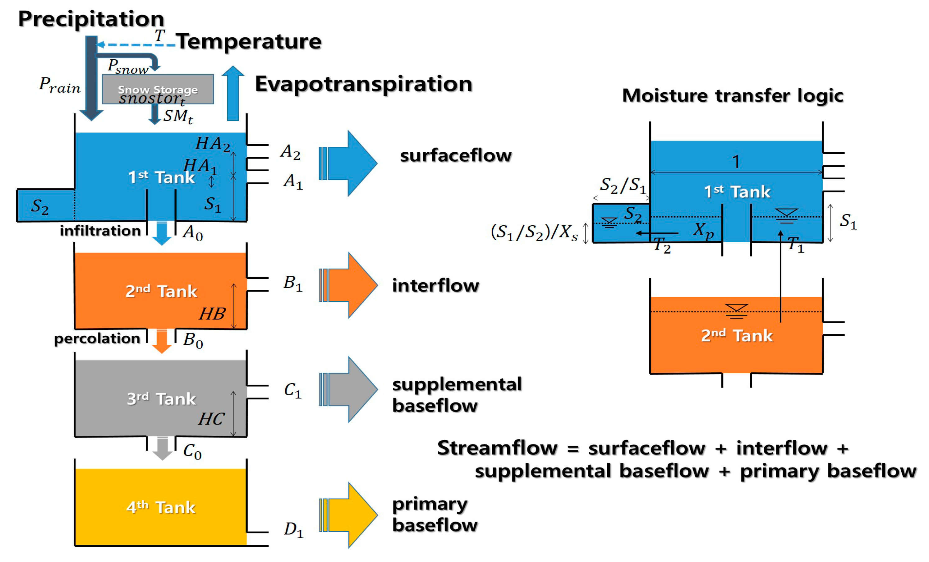
A modified conceptual rainfall-runoff model, Tank model [20] with soil moisture structure, was used as a hydrologic model for runoff simulation in this study. Having four tanks along with a soil moisture structure, the model simulates the net stream discharge as the sum of the discharges from the side outlets of the tanks. Mean areal precipitation, temperature and potential-evapotranspiration series are inputted into the model to simulate streamflow at outlet. In this study, Penman-Monteith equation was used to estimate potential-evapotranspiration [21]. Climatological records of solar radiation and humidity and wind speed are used along with temperature data. In order to consider the snow accumulation-melting module, the modified Tank model developed by McCabe and Markstrom [22] was used. Readers are referred to Sugawara [20] and McCabe and Markstrom [22] for details in terminologies and equations for all the processes. The parameters of the model are estimated using the shuffled complex evolution algorithm, one of the population-evolution-based global optimization methods [23]. Figure 2 illustrated the schematic diagram of the Tank model.
3. Application
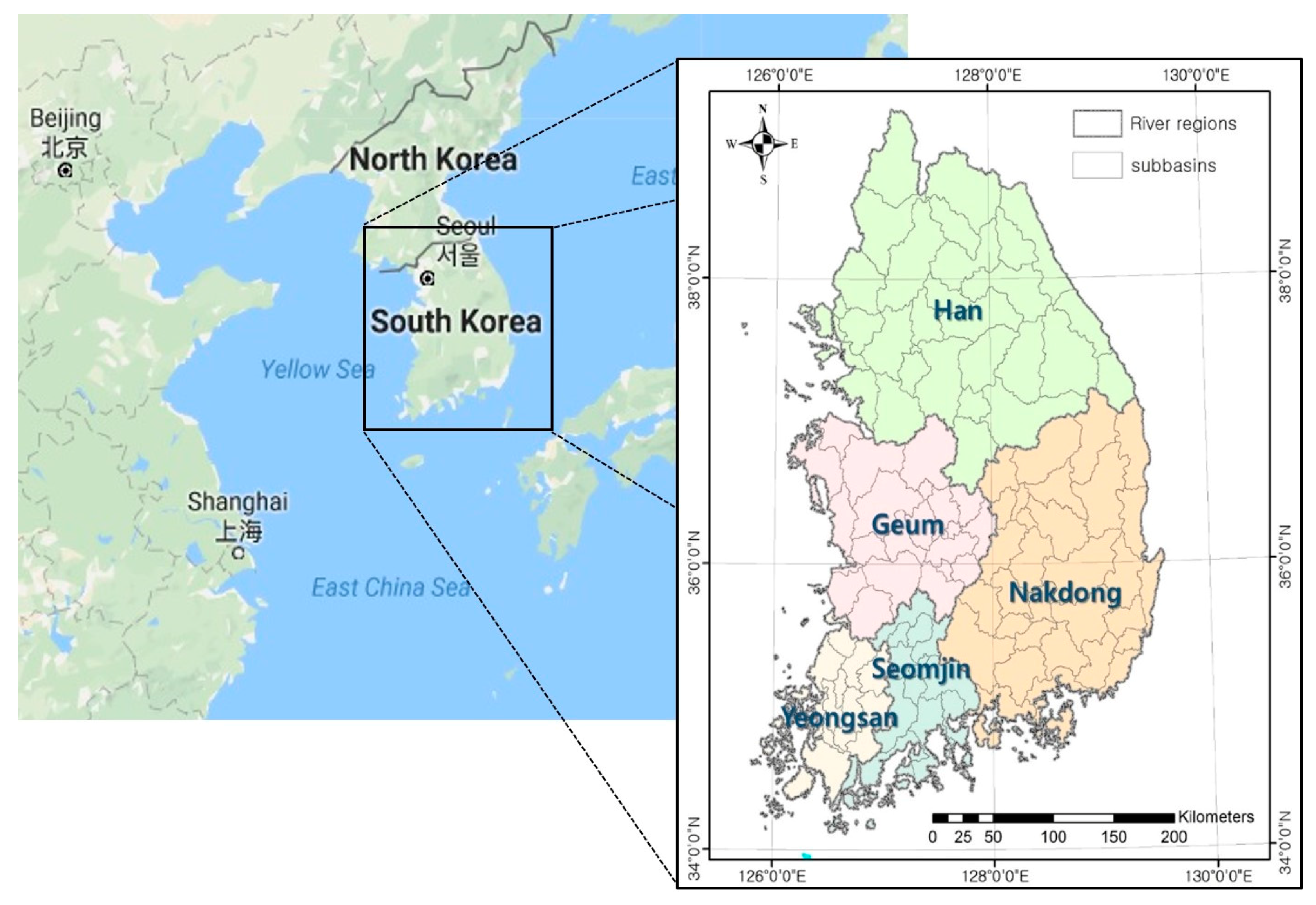
3.1. Study Area: South Korea
For a national-level application of the proposed methodology, South Korea was tested. South Korea covers an area of approximately 100,000 km2 and has a population of almost 52 million. The climatic conditions of South Korea are dominated by the Asian monsoon; therefore, approximately two-thirds of annual precipitation and runoff take place during the summer season that spans from July to September. Monsoons form the major driver behind the timing, magnitude, and distribution of wet season rainfall, rainfall inter-annual variability, and rainfall extremes in South Korea [5]. As shown in Figure 3, South Korea includes 5 major river regions and 113 subbasins (except Jeju Province). For assessment of spatial scale impacts, representative GCMs were selected for South Korea, each river region, and each subbasin separately. In other words, a single set of GCMs is selected for South Korea, five different sets of GCMs are selected for each river region, and 113 different sets of GCMs are selected for each subbasin. Mean areal climate data sets for South Korea, river regions, and subbasins are applied, respectively.
3.2. Data Sets
3.2.1. Observed Meteorological Data Sets
Observed meteorological data sets from 1976 to 2015 were obtained. Daily series of mean areal precipitation and temperature for all the subbasins were calculated using the Thiessen polygons [24] from 60 of the Korea Meteorological Administration’s Automated Surface Observing System (ASOS) gauges (https://data.kma.go.kr/data/grnd/selectAsosList.do?pgmNo=34).
3.2.2. GCM Data Sets
Historical simulation (1976–2005) and future projections, 2030s (2016–2045) and 2060s (2046–2075), of daily precipitation and temperature series were obtained from 27 GCMs of the Coupled Model Intercomparison Project Phase 5 (CMIP5) with the RCP 4.5 and 8.5 scenarios. As part of a national Research and Development (R&D) project in South Korea—“Climate Change Adaptation for Water Resources”—Asia-Pacific Economic Cooperation (APEC) Climate Center provided 27 GCMs data sets for this study. Table 2 lists the 27 GCMs applied in this study.
The coarse spatial scale of the GCMs was first interpolated to the resolution of the ASOS gauges spacing (≈45 km) based on an inverse distance weighting scheme. Mean areal values for the subbasins were subsequently calculated with the Thiessen polygons as the same as done for observed meteorological data sets. Systematic biases in these GCMs forcing data sets were corrected with Quantile Delta Mapping (QDM) approach [44]. Readers should refer to Eum and Cannon [45] for the specific steps involved in the QDM algorithm implemented for precipitation and temperature series in this study. Through the implementation of the QDM algorithm, bias-corrected values preserve relative changes in all quantiles modeled through GCMs.
3.3. Modelling Framework
Climate data sets (27 GCMs) are first pre-processed to obtain mean areal precipitation and temperature series for the three different spatial scales (national, river region, and subbasin). Then the rank of GCMs is estimated by the KKZ algorithm using the pair of climate indices for each hydrologic variable. Next, explained variabilities on climate indicators corresponding to the selected GCMs are calculated. Impacts of selected GCMs on hydrologic variables are then evaluated for the three different spatial scales as a form of explained variability of changes in hydrologic variables. Since the KKZ algorithm gives the rank of GCMs based on selection priority, by increasing the number of GCMs, corresponding explained variability are estimated. Figure 4 comprises a modelling framework of this study that illustrates the way in which the climate indices, KKZ algorithm, GCMs, Tank model, and hydrologic variables are associated and sequenced in the modelling process.
4. Results
4.1. Tank Model Parameter Estimation
Parameters of the Tank model were estimated using the observed data sets from 1976 to 2000, and the model performance was validated comparing simulated streamflow to the observed streamflow from 2001 to 2015. Daily observed streamflow (dam inflow) series from 1966 to 2016 at 35 dam sites were collected from the K-water Institute. These observed dam inflow series were used to calibrate parameters of the Tank model and the simulated streamflow series driven by the calibrated parameters were validated by comparing to the observed series. NSE values for the 35 watersheds ranged from 0.68 to 0.91, and Percent BIAS values ranged from −1.57 to 8.93.
To simulate long term streamflow for ungauged watersheds (in other words, to estimate parameters for ungauged watersheds in which observed streamflow data set does not exist), multiple regression equations were derived to estimate regional parameters of the Tank Model [46]. The six watershed characteristic factors were used as predictor variables of the regression equations. The correlation coefficients of the regional regression equations ranged from 0.64 to 0.78 [46]. As a result of the regionalization, we could be able to obtain the parameter values for all the 113 subbasins.
4.2. Selection of Representative Scenarios
GCMs were placed into different orders by the KKZ algorithm corresponding to the three hydrologic variables as introduced in Table 1. Further, these GCMs ranks were also placed differently corresponding to the three different spatial scales of climate data sets as shown in Figure 4. Table 3 and Table 4 present the rank from 1st to 5th GCMs for the three different hydrologic variables and two different spatial scales under RCP 4.5 and 8.5, respectively. Two periods of future projections, 2030s and 2060s, are presented. The GCMs rank for the subbasin scale is excluded due to difficulty in enumeration of all the subbasins.
In Table 3, bold symbols in the five river regions represent the same GCMs that are also included in the rank for national level (South Korea). Underline symbols in 2060s represents the same GCMs that are also included in 2030s. It is found that several GCMs, in general, were overlapped across different spatial scales and locations. Especially in the 2030s period, three or four out of five GCMs were overlapped. Thus, it would be anticipated that uncertainties in climate indices of finer spatial level (i.e., river region level) can be explained at some extent by the GCMs selected for coarser spatial level (i.e., national level). This premise is further discussed in Section 4.4.
Table 4 shows the rank from 1st to 5th GCMs under RCP 8.5, which are presented based on the same fashion in Table 3, but red-colored symbols represent the same GCMs that are also included under RCP 4.5. Interestingly, only a few GCMs (one or two GCMs out of the five) were overlapped between RCP 4.5 and 8.5. There was no general agreement on selected GCMs between RCP 4.5 and 8.5. Given that RCP 8.5 represents the business as usual scenario whereas RCP 4.5 represents the possible mitigation measure scenario, the selection of representative climate scenarios should be carefully implemented under various hypotheses on the future adaptation strategies.
4.3. Explained Variability on Climate Indices
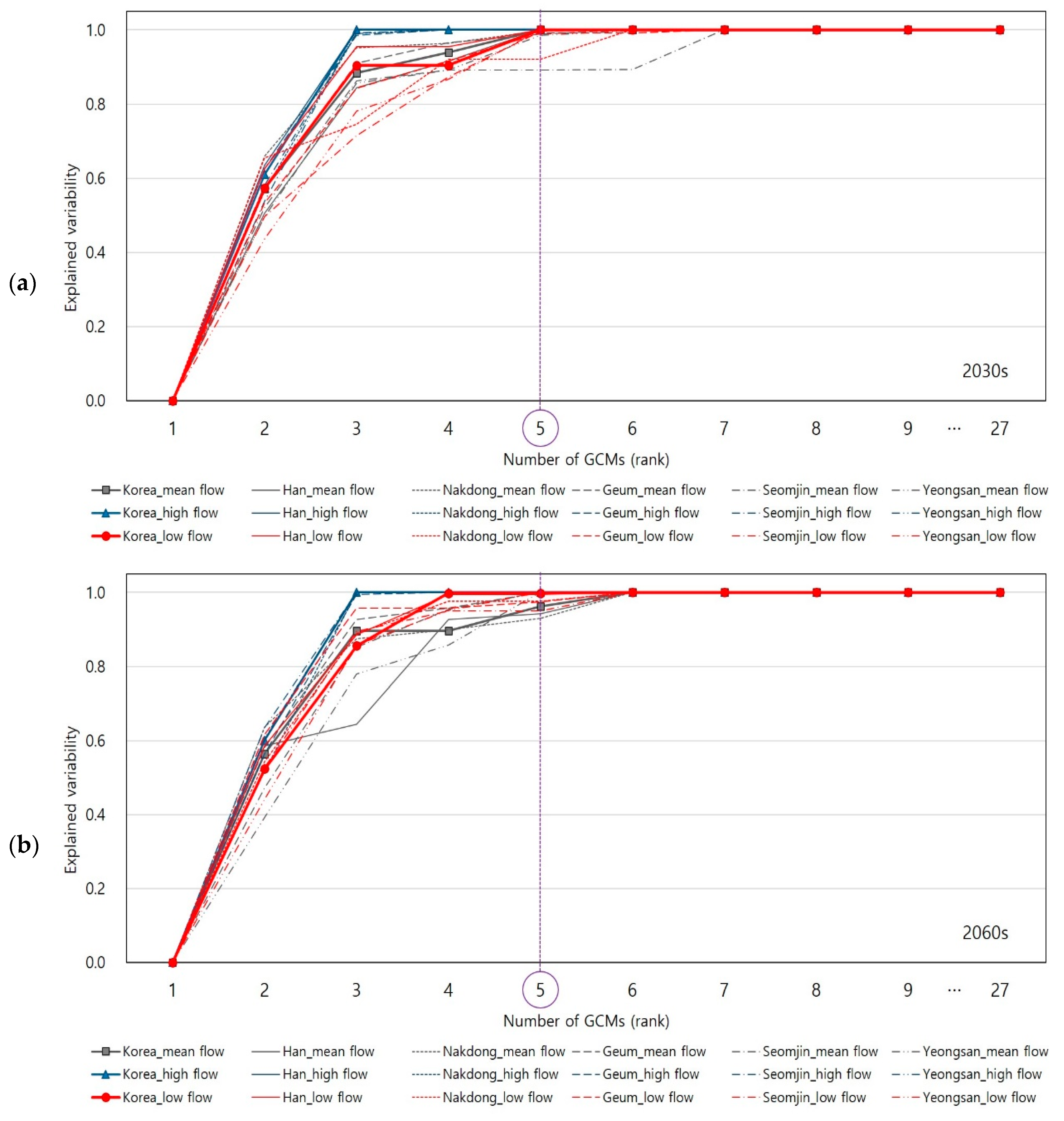
Although Table 3 and Table 4 only show the selected GCMs to the 5th rank, the KKZ algorithm makes the entire GCMs ordered according to their priority. Figure 5 and Figure 6 present explained variability of changes in climate indices for 2030s and 2060s periods under RCP 4.5 and RCP 8.5 scenarios, respectively.
As shown in Figure 5 and Figure 6, it is found that total 80% of explained variability (presented on y-axis) was quickly arrived by only the three of four GCMs (presented on x-axis). Further, the majority (close to 100% of) of explained variability was arrived by the five GCMs in most cases. Thus, the KKZ algorithm successfully identified the top five GCMs (among 27) that are able to explain the majority of inter-model variability from all the GCMs.
4.4. Explained Variability on Hydrologic Variables
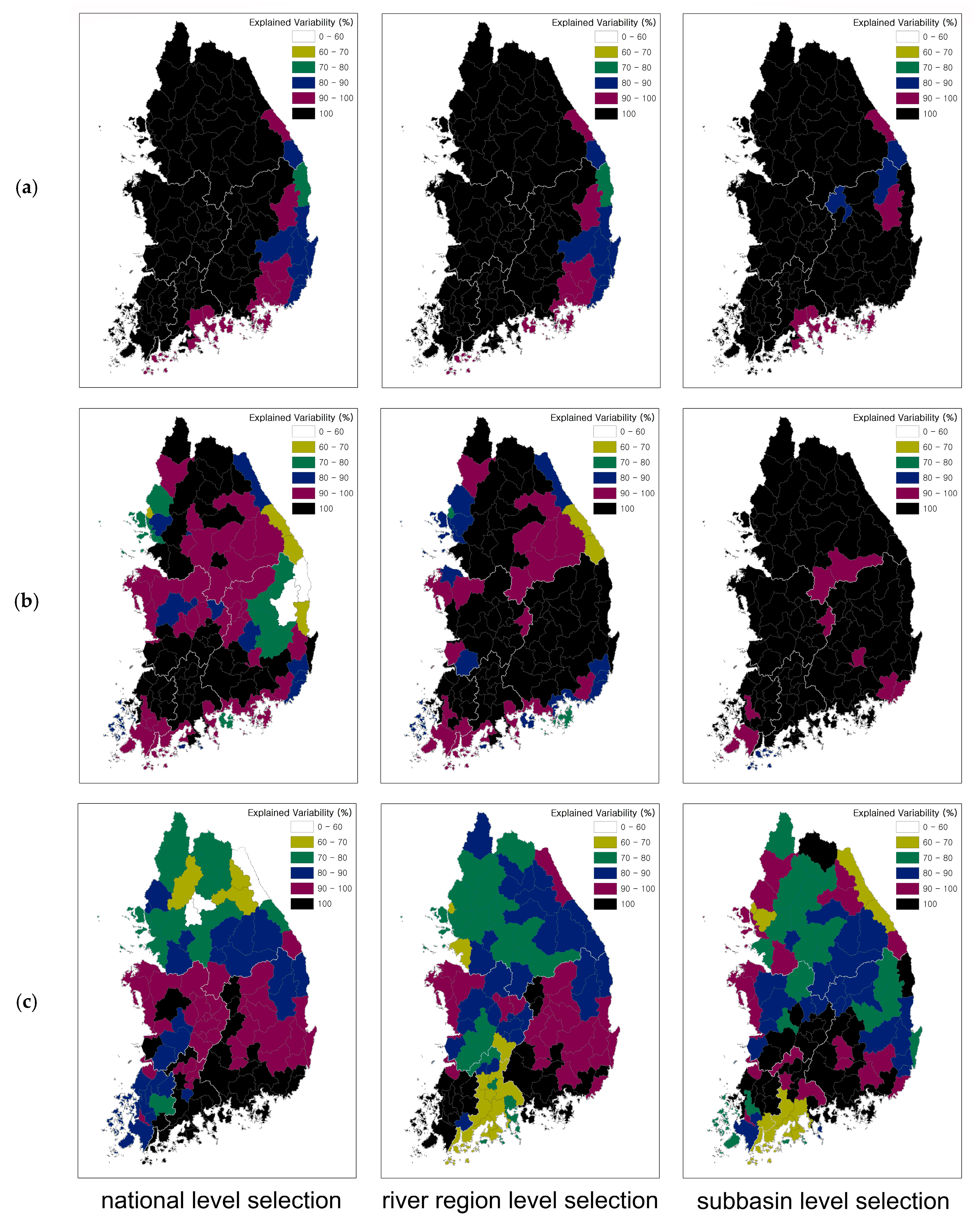
Since the majority (more than 80%) of inter-model variability from all the GCMs were successfully explained under both the RCP 4.5 and 8.5, the results of explained variability on hydrologic variables under RCP 4.5 are presented in this section. We do not present the results from RCP 8.5 because the both RCP 4.5 and 8.5 output very similar results. Figure 7 presents the explained variabilities of changes in three hydrologic variables (mean flow, high flow, and low flow) in the 2030s period under RCP 4.5. The explained variabilities were calculated for all the 113 subbasins using the top five GCMs that are ranked by the KKZ algorithm. The explained variabilities in the figures on the left, middle, and right were estimated by the GCMs ranked by the national, river region, and subbasin level of climate data sets, respectively. In other words, the explained variabilities of all the subbasins were estimated by the same set of top five GCMs ranked by the national level selection (on the left) while the explained variability of each subbasin was estimated by each set of top five GCMs ranked by the subbasin level selection (on the right). The explained variabilities of all the subbasins that consist of the same river region were estimated by the same set of top five GCMs ranked by the river region level selection (on the middle).
In general, explained variablilities of changes in mean flow (Figure 7a) was well preserved by the top five GCMs regardless of spatial scale of climate data sets. It is found that only one set of 5 GCMs has capability of capturing almost the whole inter-model variability driven by the 27 GCMs. In case of high flow (Figure 7b), although inter-model variabilities were not sufficiently explained by the national level selection in a few subbasins (on the left), when it comes to the subbasin level selection (on the right), most of inter-model variabilities were successfully explained. There was similar pattern in Figure 7c though the explained variabilities were relatively lesser then the above two variables (Figure 7a,b). Thus, when we used finer scale of climate data sets for the KKZ algorithm, the transferability of the selected GCMs to uncertainty in hydrological impacts was increased. Nonetheless, note that a single set of GCMs ranked by the national level selection also has remarkable ability to explain inter-model variability of changes in hydrologic variables on each subbasin.
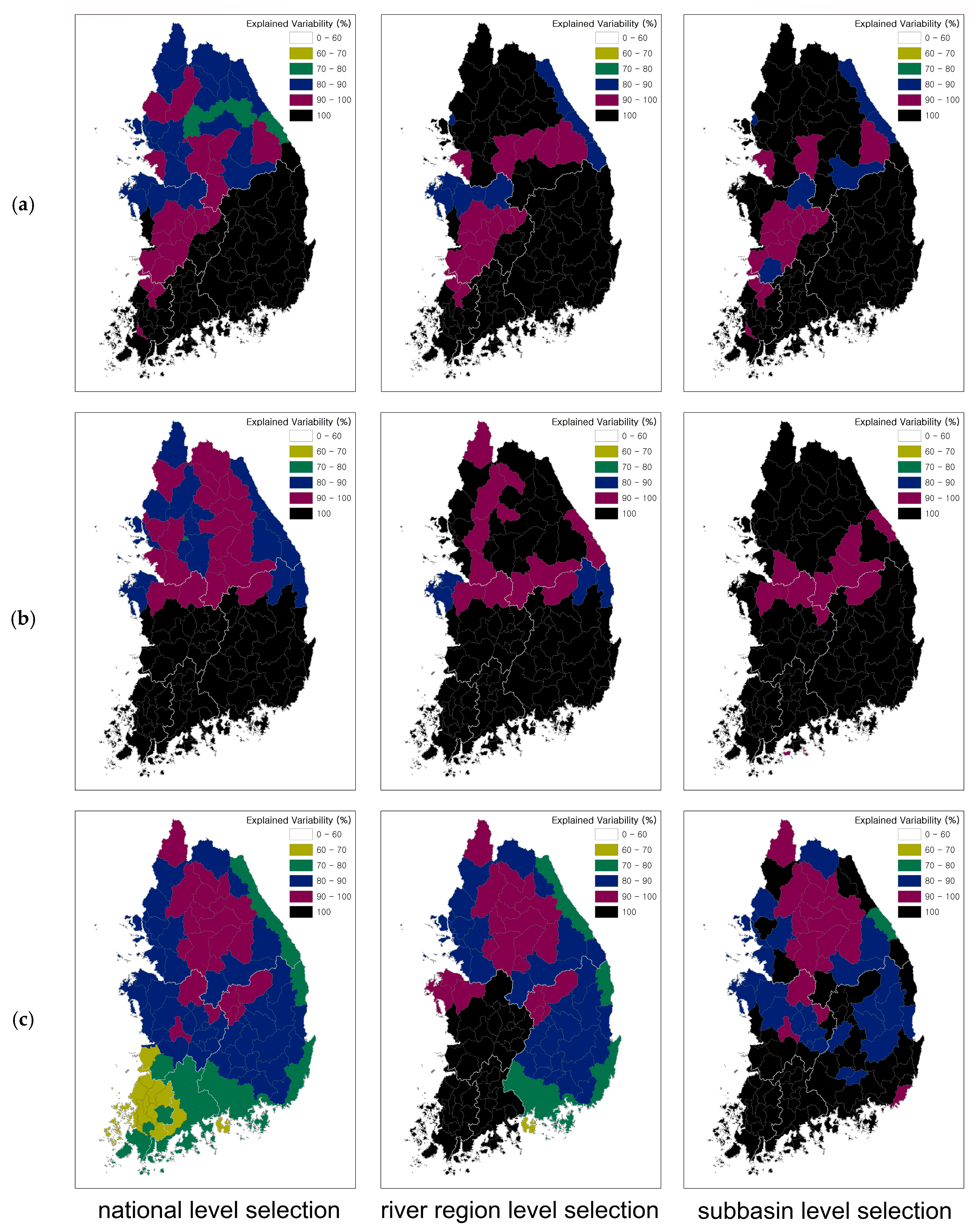
Figure 8 shows the explained variabilities of changes in three hydrologic variables (mean flow, high flow, and low flow) in the 2060s period under RCP 4.5 for the 113 subbasins. Similar to the 2030s period, the explained variabilities of changes in mean flow and high flow (Figure 8a,b) were well preserved by the top five GCMs regardless of spatial scale of climate data sets except the Han river region. Nonetheless, explained variabilities of changes in mean flow and high flow in the Han river region were also well preserved under river region and subbasin level selection. Similarly, in case of changes in low flow, although explained variabilities were relatively low in the Seomjin and Yeongsan river regions, they were also well preserved under river region and subbasin level selections. Thus, it shows that the transferability of the selected GCMs to uncertainty in local-scale hydrological impacts studies can be improved by using finer scale of climate data sets for the KKZ algorithm. In terms of spatial scale of climate data sets for selection of GCMs, it is found that a single set of top five GCMs (i.e., the five GCMs selected for national level, South Korea) can explain almost the whole range of inter-model variabilities except a few subbasins in case of changes in mean and high flow although it may not be applicable to changes in low flow.
Regarding the findings, final suggestion on the representative climate change scenarios for South Korea were determined as shown in Table 5 and Table 6 for 2030s and 2060s future period, respectively, under RCP 4.5. Note that we chose the RCP 4.5 as a realistic future scenario since it represent the possible mitigation measure unlike the RCP 8.5, which represents the worst case for the climate change adaptation. For climate change impact studies on mean flow and high flow variables, a single set of GCMs was assigned for all the 113 subbasins for each future period. For low flow variable, on the other hand, the five different sets of GCMs were assigned to the subbasins belonging to the five river regions, respectively. Based on the selecting process of the KKZ algorithm, the 1st GCM represents the centroid across all the ensemble members so that the first GCM can represent the median of changes in the hydrologic variable. From the second selection, on the other hand, since the GCM that lies farthest from the previous selection(s) is selected, the 2nd to the 5th GCMs represent the values close to either the maximum or minimum changes in the hydrologic variable. Thus, by considering these top five GCMs selected by the KKZ algorithm, almost the whole inter-model variabilities of changes in hydrologic variables can be explained.
5. Conclusions
Appropriate spatial scales for the selection of representative climate scenarios were analyzed in this study with a case study for South Korea. Overall, in case of such a small country like South Korea (approximately 0.1 million km2), a single set of representative GCMs would be able to capture inter-model variabilities of hydrologic variables for local-level impact studies. However, for low flow variable, finer scale of GCMs selection would be required considering different sets for each local-level case studies. Furthermore, the representative GCMs need to be selected separately for different future periods since uncertainties in GCMs get larger with lead time, which is consistent with the previous study by Hawkins and Sutton [47].
We found that the inter-model variabilities of changes in hydrologic variables are well preserved by only a single set of GCMs (i.e., the top five GCMs from the total 27 in this study). This can certainly reduce computational burden on water resources planning and management studies for which potential uncertainties in climate change should be addressed [48]. However, for local-scale hydrologic impact studies (i.e., subbasin level in this study), decision makers may have difficulty in determining which set of GCMs they should use. If only a single set of GCMs is provided, they do not have to worry about which scenarios to use. On the contrary, different sets of GCMs are provided for each subbasin, which would hinder easy implementation of GCMs for local-scale studies.
Nonetheless, given that a single set of GCMs ranked by the national level selection has the remarkable ability to capture potential inter-model variabilities of changes in mean and high flow variables, the single set of representative climate scenarios can provide sufficient information on uncertainties in future changes in mean- and high-flow regimes. Only for low flow variables would a certain set of GCMs selected by finer spatial scale of climate data sets that are specified for local basins of interest be required for better understanding of uncertainties in future changes in the low flow regimes.
Furthermore, we found that different sets of GCMs were selected for the two different future periods (the 2030s and 2060s in this study). This implies that utilization of the same set of GCMs selected for near-term future would not be reliable for long-term future. Since relative importance of uncertainties in GCMs increases with time [47], it seems reasonable that different sets of GCMs have to be selected for the near-term and long-term future period separately. In addition, different sets of GCMs were selected under two different RCP scenarios (4.5 and 8.5). This implies that different sets of representative GCMs can be selected according to what assumption on the future adaptation strategy would be considered.
We should note that the area of national-level application tested in this study, South Korea, is relatively small. When a national-level application is implemented on much wider nations, such as United States (USA), China, and Australia, spatial heterogeneity on climate data sets would diminish due to smoothing impact driven by averaging climate data sets on multiple locations. In these cases, sub-national level (e.g., states in USA) selection can be recommended for the selection of representative climate change scenarios.
Author Contributions
S.B.S. mainly contributed to the design and development of this manuscript. The manuscript has written by S.B.S. with contribution from Y.-O.K.
Funding
This research was funded by the National Research Foundation of Korea (grant number is NRF-2017R1A6A3A11031800).
Acknowledgments
This research was supported by a grant (NRF-2017R1A6A3A11031800) through the Young Researchers program funded by the National Research Foundation of Korea. This research was also supported by a grant (2014001310007) from the Climate Change Correspondence Program funded by the Ministry of Environment in Korea. The authors thank the Climate Change Adaptation for Water Resources (CCAW) research center and the APEC Climate Center for providing the 27 GCMs data sets.
Conflicts of Interest
The authors declare no conflict of interest.
References
- Seo, S.B.; Kim, Y.-O.; Kim, Y.; Eum, H.-I. Selecting climate change scenarios for regional hydrologic impact studies based on climate extreme indices. Clim. Dyn. 2018. [Google Scholar] [CrossRef]
- Dubrovsky, M.; Trnka, M.; Holman, I.P.; Svobodova, E.; Harrison, P.A. Developing a reduced-form ensemble of climate change scenarios for Europe and its application to selected impact indicators. Clim. Chang. 2015, 128, 169–186. [Google Scholar] [CrossRef]
- Lee, J.-K.; Kim, Y.-O. Selecting climate change scenarios reflecting uncertainties. Atmosphere 2012, 22, 149–161. [Google Scholar] [CrossRef]
- Knutti, R.; Masson, D.; Gettelman, A. Climate model genealogy: Generation CMIP5 and how we got there. Geophys. Res. Lett. 2013, 40, 1194–1199. [Google Scholar] [CrossRef] [Green Version]
- McSweeney, C.F.; Jones, R.G.; Booth, B.B.B. Selecting ensemble members to provide regional climate change information. J. Clim. 2012, 25, 7100–7121. [Google Scholar] [CrossRef]
- Masson, D.; Knutti, R. Climate model genealogy. Geophys. Res. Lett. 2011, 38, L08703. [Google Scholar] [CrossRef]
- Mendlik, T.; Gobiet, A. Selecting climate simulations for impact studies based on multivariate patterns of climate change. Clim. Chang. 2016, 135, 381–393. [Google Scholar] [CrossRef] [PubMed]
- Wilcke, R.A.I.; Bärring, L. Selecting regional climate scenarios for impact modelling studies. Environ. Model. Softw. 2016, 78, 191–201. [Google Scholar] [CrossRef]
- Mote, P.W.; Salathé, E.P. Future climate in the Pacific Northwest. Clim. Chang. 2010, 102, 29–50. [Google Scholar] [CrossRef] [Green Version]
- Rupp, D.E.; Abatzoglou, J.T.; Hegewisch, K.C.; Mote, P.W. Evaluation of CMIP5 20th century climate simulations for the Pacific Northwest USA. J. Geophys. Res. Atmos. 2013, 118, 10884–10906. [Google Scholar] [CrossRef]
- Vano, J.A.; Kim, J.B.; Rupp, D.E.; Mote, P.W. Selecting climate change scenarios using impact-relevant sensitivities. Geophys. Res. Lett. 2015, 42, 5516–5525. [Google Scholar] [CrossRef] [Green Version]
- Cannon, A.J. Selecting GCM scenarios that span the range of changes in a multimodel ensemble: Application to CMIP5 climate extremes indices. J. Clim. 2015, 28, 1260–1267. [Google Scholar] [CrossRef]
- Houle, D.; Bouffard, A.; Duchesne, L.; Logan, T.; Harvey, R. Projections of future soil temperature and water content for three southern quebec forested sites. J. Clim. 2012, 25, 7690–7701. [Google Scholar] [CrossRef]
- Katsavounidis, I.; Kuo, C.C.J.; Zhang, Z. A new initialization technique for generalized Lloyd iteration. IEEE Signal Process. Lett. 1994, 1, 144–146. [Google Scholar] [CrossRef]
- Chen, J.; Brissette, F.P.; Lucas-Picher, P. Transferability of optimally-selected climate models in the quantification of climate change impacts on hydrology. Clim. Dyn. 2016, 47, 3359–3372. [Google Scholar] [CrossRef]
- Zhang, X.; Alexander, L.; Hegerl, G.C.; Jones, P.; Tank, A.K.; Peterson, T.C.; Trewin, B.; Zwiers, F.W. Indices for monitoring changes in extremes based on daily temperature and precipitation data. WIREs Clim. Chang. 2011, 2, 851–870. [Google Scholar] [CrossRef]
- Kustu, M.D.; Fan, Y.; Robock, A. Large-scale water cycle perturbation due to irrigation pumping in the US High Plains: A synthesis of observed streamflow changes. J. Hydrol. 2010, 390, 222–244. [Google Scholar] [CrossRef]
- Wang, H.; Brill, E.D.; Ranjithan, R.S.; Sankarasubramanian, A. A framework for incorporating ecological releases in single reservoir operation. Adv. Water Resour. 2015, 78, 9–21. [Google Scholar] [CrossRef]
- Woolfenden, R.; Nishikawa, T. Simulation of Groundwater and Surface-Water Resources of the Santa Rosa Plain Watershed, Sonoma County, California; Scientific Investigations Report; US Geological Survey: Reston, VA, USA, 2014.
- Sugawara, M. Tank model. In Computer Models of Watershed Hydrology; Water Resources Publications: Littleton, CO, USA, 1995. [Google Scholar]
- Cai, J.; Liu, Y.; Lei, T.; Pereira, L.S. Estimating reference evapotranspiration with the FAO Penman–Monteith equation using daily weather forecast messages. Agric. For. Meteorol. 2007, 145, 22–35. [Google Scholar] [CrossRef]
- McCabe, G.J.; Markstrom, S.L. A Monthly Water-Balance Model Driven by a Graphical User Interface (No. 2007-1088); Geological Survey (US): Reston, VA, USA, 2007.
- Duan, Q.; Sorooshian, S.; Gupta, V. Effective and efficient global optimization for conceptual rainfall-runoff models. Water Resour. Res. 1992, 28, 1015–1031. [Google Scholar] [CrossRef]
- Thiessen, A. Precipitations averages for large areas. Mon. Weather Rev. 1911, 39, 1082–1089. [Google Scholar] [CrossRef]
- Wu, T. A mass-flux cumulus parameterization scheme for large-scale models: Description and test with observations. Clim. Dyn. 2012, 38, 725–744. [Google Scholar] [CrossRef]
- Chylek, P.; Li, J.; Dubey, M.K.; Wang, M.; Lesins, G. Observed and model simulated 20th century Arctic temperature variability: Canadian Earth System Model CanESM2. Atmos. Chem. Phys. Discuss. 2011, 11, 22893–22907. [Google Scholar] [CrossRef]
- Gent, P.R.; Danabasoglu, G.; Donner, L.J.; Holland, M.M.; Hunke, E.C.; Jayne, S.R.; Lawrence, D.M.; Neale, R.B.; Rasch, P.J.; Vertenstein, M.; et al. The Community Climate System Model Version 4. J. Clim. 2011, 24, 4973–4991. [Google Scholar] [CrossRef] [Green Version]
- Moore, J.K.; Lindsay, K.; Doney, S.C.; Long, M.C.; Misumi, K. Marine ecosystem dynamics and biogeochemical cycling in the Community Earth System Model [CESM1(BGC)]: Comparison of the 1990s with the 2090s under the RCP4.5 and RCP8.5 Scenarios. J. Clim. 2013, 26, 9291–9312. [Google Scholar] [CrossRef]
- Meehl, G.A.; Washington, W.M.; Arblaster, J.M.; Hu, A.; Teng, H.; Kay, J.E.; Gettelman, A.; Lawrence, D.M.; Sanderson, B.M.; Strand, W.G. Climate change projections in CESM1(CAM5) compared to CCSM4. J. Clim. 2013, 26, 6287–6308. [Google Scholar] [CrossRef]
- Scoccimarro, E.; Gualdi, S.; Bellucci, A.; Sanna, A.; Giuseppe Fogli, P.; Manzini, E.; Vichi, M.; Oddo, P.; Navarra, A. Effects of tropical cyclones on ocean heat transport in a high-resolution coupled general circulation model. J. Clim. 2011, 24, 4368–4384. [Google Scholar] [CrossRef]
- Davini, P.; Cagnazzo, C.; Fogli, P.G.; Manzini, E.; Gualdi, S.; Navarra, A. European blocking and Atlantic jet stream variability in the NCEP/NCAR reanalysis and the CMCC-CMS climate model. Clim. Dyn. 2014, 43, 71–85. [Google Scholar] [CrossRef]
- Voldoire, A.; Sanchez-Gomez, E.; Salas y Mélia, D.; Decharme, B.; Cassou, C.; Sénési, S.; Valcke, S.; Beau, I.; Alias, A.; Chevallier, M.; et al. The CNRM-CM5.1 global climate model: Description and basic evaluation. Clim. Dyn. 2013, 40, 2091–2121. [Google Scholar] [CrossRef] [Green Version]
- Bao, Q.; Lin, P.; Zhou, T.; Liu, Y.; Yu, Y.; Wu, G.; He, B.; He, J.; Li, L.; Li, J.; et al. The Flexible Global Ocean-Atmosphere-Land system model, Spectral Version 2: FGOALS-s2. Adv. Atmos. Sci. 2013, 30, 561–576. [Google Scholar] [CrossRef]
- Dunne, J.P.; John, J.G.; Adcroft, A.J.; Griffies, S.M.; Hallberg, R.W.; Shevliakova, E.; Stouffer, R.J.; Cooke, W.; Dunne, K.A.; Harrison, M.J.; et al. GFDL’s ESM2 Global Coupled Climate–Carbon Earth System Models. Part I: Physical formulation and baseline simulation characteristics. J. Clim. 2012, 25, 6646–6665. [Google Scholar] [CrossRef]
- Schmidt, G.A.; Kelley, M.; Nazarenko, L.; Ruedy, R.; Russell, G.L.; Aleinov, I.; Bauer, M.; Bauer, S.E.; Bhat, M.K.; Bleck, R.; et al. Configuration and assessment of the GISS ModelE2 contributions to the CMIP5 archive. J. Adv. Model Earth Syst. 2014, 6, 141–184. [Google Scholar] [CrossRef] [Green Version]
- Collins, W.J.; Bellouin, N.; Doutriaux-Boucher, M.; Gedney, N.; Halloran, P.; Hinton, T.; Hughes, J.; Jones, C.D.; Joshi, M.; Liddicoat, S.; et al. Development and evaluation of an Earth-System model—HadGEM2. Geosci. Model Dev. 2011, 4, 1051–1075. [Google Scholar] [CrossRef]
- Volodin, E.M.; Dianskii, N.A.; Gusev, A.V. Simulating present-day climate with the INMCM4.0 coupled model of the atmospheric and oceanic general circulations. Izv. Atmos. Ocean Phys. 2010, 46, 414–431. [Google Scholar] [CrossRef]
- Dufresne, J.-L.; Foujols, M.-A.; Denvil, S.; Caubel, A.; Marti, O.; Aumont, O.; Balkanski, Y.; Bekki, S.; Bellenger, H.; Benshila, R.; et al. Climate change projections using the IPSL-CM5 Earth System Model: From CMIP3 to CMIP5. Clim. Dyn. 2013, 40, 2123–2165. [Google Scholar] [CrossRef] [Green Version]
- Tatebe, H.; Ishii, M.; Mochizuki, T.; Chikamoto, Y.; Sakamoto, T.T.; Komuro, Y.; Mori, M.; Yasunaka, S.; Watanabe, M.; Ogochi, K.; et al. The initialization of the MIROC climate models with hydrographic data assimilation for decadal prediction. J. Meteorol. Soc. Jpn. 2012, 90A, 275–294. [Google Scholar] [CrossRef]
- Watanabe, S.; Hajima, T.; Sudo, K.; Nagashima, T.; Takemura, T.; Okajima, H.; Nozawa, T.; Kawase, H.; Abe, M.; Yokohata, T.; et al. MIROC-ESM 2010: Model description and basic results of CMIP5-20c3m experiments. Geosci. Model Dev. 2011, 4, 845–872. [Google Scholar] [CrossRef]
- Giorgetta, M.A.; Jungclaus, J.; Reick, C.H.; Legutke, S.; Bader, J.; Böttinger, M.; Brovkin, V.; Crueger, T.; Esch, M.; Fieg, K.; et al. Climate and carbon cycle changes from 1850 to 2100 in MPI-ESM simulations for the Coupled Model Intercomparison Project phase 5. J. Adv. Model Earth Syst. 2013, 5, 572–597. [Google Scholar] [CrossRef] [Green Version]
- Yukimoto, S.; Adachi, Y.; Hosaka, M.; Sakami, T.; Yoshimura, H.; Hirabara, M.; TANAKA, T.Y.; Shindo, E.; Tsujino, H.; Deushi, M.; et al. A new global climate model of the Meteorological Research Institute: MRI-CGCM3—Model description and basic performance. J. Meteorol. Soc. Jpn. 2012, 90A, 23–64. [Google Scholar] [CrossRef]
- Bentsen, M.; Bethke, I.; Debernard, J.B.; Iversen, T.; Kirkevåg, A.; Seland, Ø.; Drange, H.; Roelandt, C.; Seierstad, I.A.; Hoose, C.; et al. The Norwegian Earth System Model, NorESM1-M—Part 1: Description and basic evaluation of the physical climate. Geosci. Model Dev. 2013, 6, 687–720. [Google Scholar] [CrossRef]
- Cannon, A.J.; Sobie, S.R.; Murdock, T.Q. Bias correction of GCM precipitation by quantile mapping: How well do methods preserve changes in quantiles and extremes? J. Clim. 2015, 28, 6938–6959. [Google Scholar] [CrossRef]
- Eum, H.-I.; Cannon, A.J. Intercomparison of projected changes in climate extremes for South Korea: Application of trend preserving statistical downscaling methods to the CMIP5 ensemble. Int. J. Climatol. 2017, 37, 3381–3397. [Google Scholar] [CrossRef]
- Lee, S.H.; Kang, S.U. A parameter regionalization study of a modified Tank model using characteristic factors of watersheds. J. Korean Soc. Civ. Eng. 2007, 27, 379–385. [Google Scholar]
- Hawkins, E.; Sutton, R. The potential to narrow uncertainty in regional climate predictions. Bull. Am. Meteorol. Soc. 2009, 90, 1095–1107. [Google Scholar] [CrossRef]
- Seo, S.B.; Sinha, T.; Mahinthakumar, G.; Sankarasubramanian, A.; Kumar, M. Identification of dominant source of errors in developing streamflow and groundwater projections under near-term climate change. J. Geophys. Res. Atmos. 2016, 121, 7652–7672. [Google Scholar] [CrossRef]
Figure 1.
A selection procedure of the Katsavounidis-Kuo-Zhang (KKZ) algorithm with a simple example of two climate variables [1]: (a) Step (3)—select 3rd GCM having the longest distance among a group of shortest distances to either the 1st or 2nd Global Circulation Model (GCM); (b) Step (4)—select 4th GCM having the longest distance among a group of shortest distances to among the 1st to 3rd GCMs; (c) Step (4)—select 5th GCM having the longest distance among a group of shortest distances to among the 1st to 4th GCMs. Here, the gray arrows represent GCMs disregarded by the algorithm.
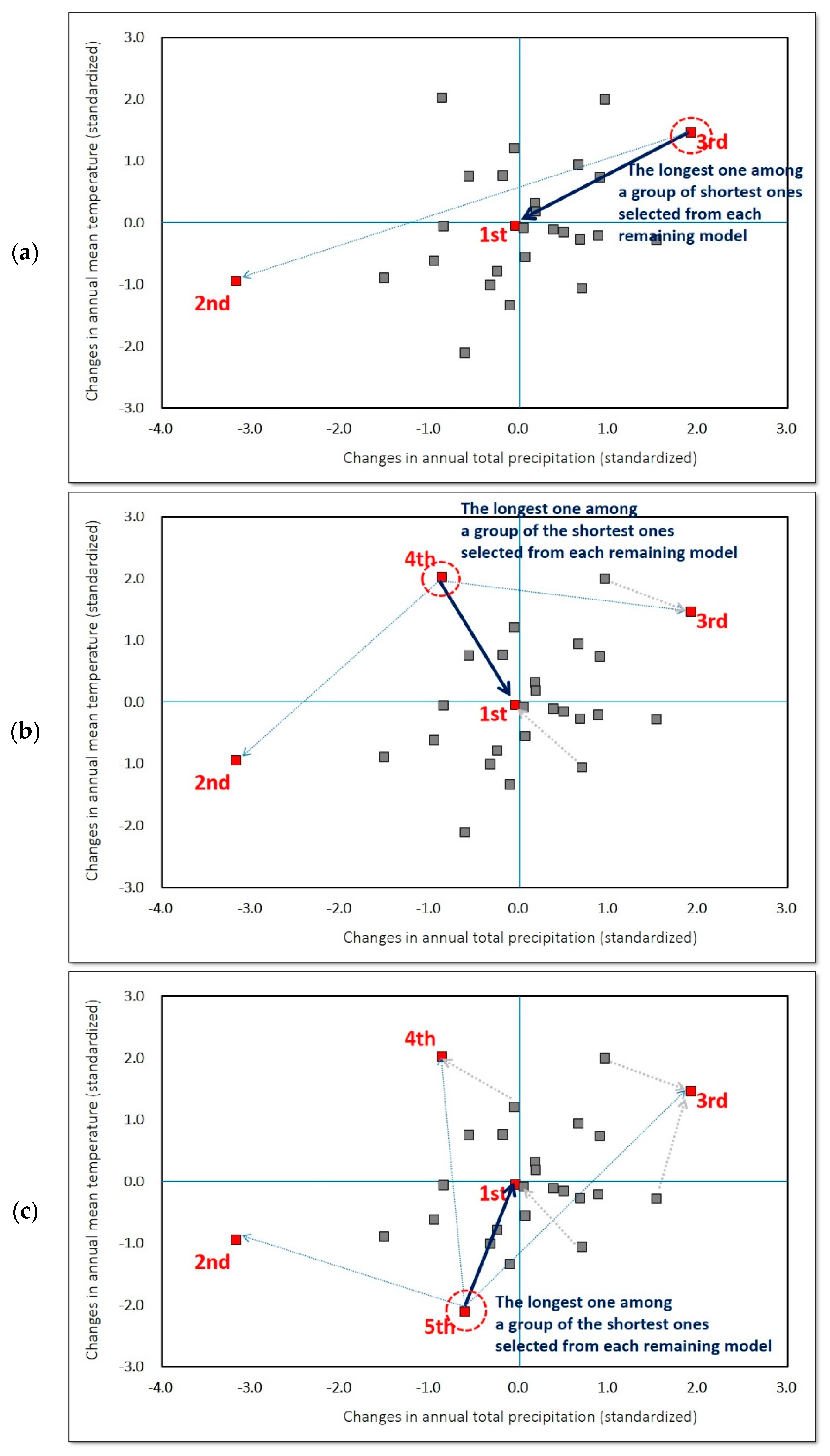
Figure 2.
Schematic diagram of the Tank model. T: temperature; Prain: rainfall; Psnow: snow; snostor: snow storage; SM: snow melt.
Figure 2.
Schematic diagram of the Tank model. T: temperature; Prain: rainfall; Psnow: snow; snostor: snow storage; SM: snow melt.

Figure 3.
A study area: South Korea, which includes 5 river regions and 113 subbasins.

Figure 4.
A diagram of modelling framework of this study. (PRCP: precipitation, TEMP: temperature).
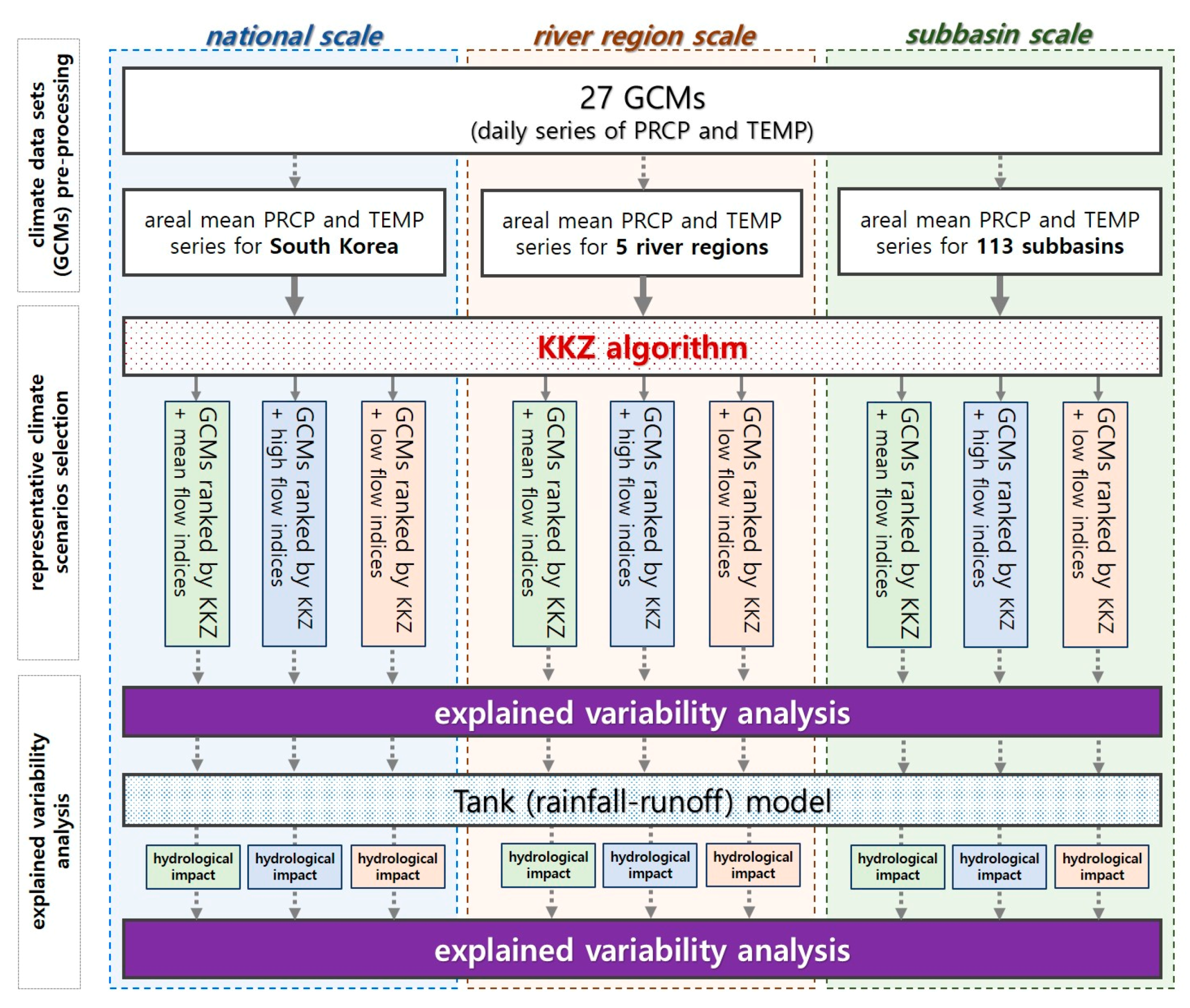
Figure 5.
The explained variability of changes in climate indices according to the number of GCMs that are ranked by the KKZ under RCP 4.5. The thinner lines of each color are estimated using mean areal climate data for each river region, while the thicker lines with markers are estimated using mean areal climate data for national level: (a) explained variability of changes in climate indices for 2030s period under RCP 4.5; (b) explained variability of changes in climate indices for the 2060s period under RCP 4.5.

Figure 6.
The explained variability of changes in climate indices according to the number of GCMs that are ranked by the KKZ under RCP 8.5. The thinner lines of each color are estimated using mean areal climate data for each river region, while the thicker lines with markers are estimated using mean areal climate data for national level: (a) explained variability of changes in climate indices for the 2030s period under RCP 8.5; (b) explained variability of changes in climate indices for the 2060s period under RCP 8.5.
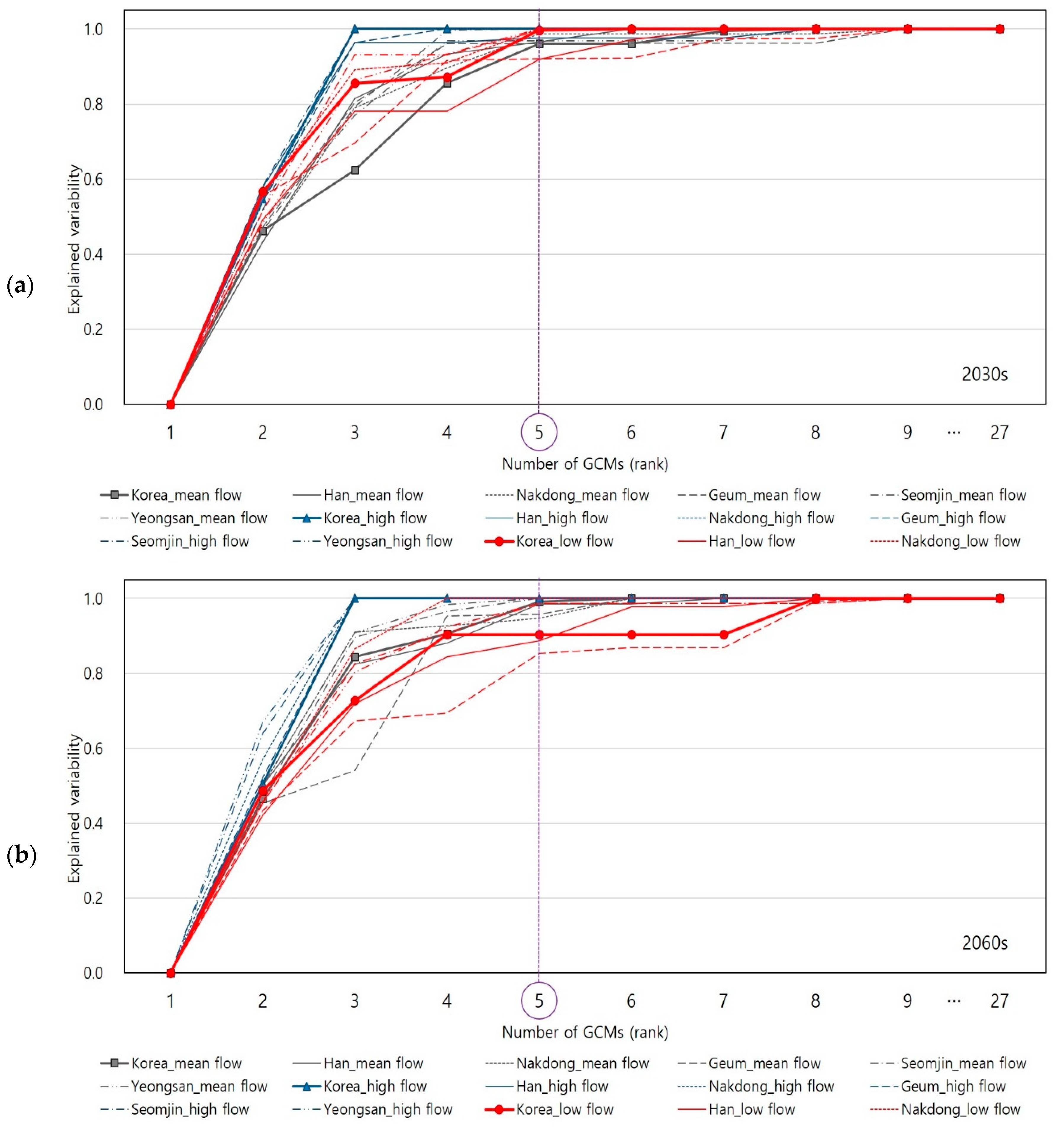
Figure 7.
The explained variabilities of changes in hydrologic variables (mean flow, high flow, and low flow) in the 2030s period under RCP 4.5 for the 113 subbasins. The results in the first, the second, and the third column from the left were estimated by the top five GCMs selected using the national level, river region level, and subbasin level of climate data sets, respectively: (a) mean flow; (b) high flow; (c) low flow.

Figure 8.
The explained variabilities of changes in hydrologic variables (mean flow, high flow, and low flow) in the 2060s period under RCP 4.5 for the 113 subbasins. The results in the first, second, and third column from the left were estimated by the top five GCMs selected using the national level, river region level, and subbasin level of climate data sets, respectively: (a) mean flow; (b) high flow; (c) low flow.


Table 1.
Pairs of climate indices for the three hydrologic categories (variables).
| Category | Index | Description | Change |
|---|---|---|---|
| mean flow | PRCPTOT | Annual total precipitation in wet days | % |
| MEANTEMP | Annual mean temperature (°C) | ||
| high flow | Rx5day PRCP | Annual maximum consecutive 5-day precipitation (mm) | % |
| Rx3day PRCP | Annual maximum consecutive 3-day precipitation (mm) | % | |
| low flow | DTR | Annual mean difference between daily max temperature and min temperature (°C) | |
| Rn30day PRCP | Annual minimum consecutive 30-day precipitation (mm) | % |
Table 2.
The list of climate models used in this study: 27 GCMs under Representative Concentration Pathways (RCP) 4.5 and 8.5.
Table 2.
The list of climate models used in this study: 27 GCMs under Representative Concentration Pathways (RCP) 4.5 and 8.5.
| No. | Model | Resolution [Degrees] | Reference |
|---|---|---|---|
| 1 | BCC-CSM1-1 | 2.813 × 2.791 | Wu [25] |
| 2 | BCC-CSM1-1-M | 1.125 × 1.122 | Wu [25] |
| 3 | CanESM2 | 2.813 × 2.791 | Chylek et al. [26] |
| 4 | CCSM4 | 1.250 × 0.942 | Gent et al. [27] |
| 5 | CESM1-BGC | 1.250 × 0.942 | Moore et al. [28] |
| 6 | CESM1-CAM5 | 1.250 × 0.942 | Meehl et al. [29] |
| 7 | CMCC-CM | 0.750 × 0.748 | Scoccimarro et al. [30] |
| 8 | CMCC-CMS | 1.875 × 1.865 | Davini et al. [31] |
| 9 | CNRM-CM5 | 1.406 × 1.401 | Voldoire et al. [32] |
| 10 | FGOALS-s2 | 2.813 × 1.659 | Bao et al. [33] |
| 11 | GFDL-ESM2G | 2.500 × 2.023 | Dunne et al. [34] |
| 12 | GFDL-ESM2M | 2.500 × 2.023 | Dunne et al. [34] |
| 13 | GISS-E2-R | 2.000 × 2.500 | Schmidt et al. [35] |
| 14 | HadGEM2-AO | 1.875 × 1.250 | Collins et al. [36] |
| 15 | HadGEM2-CC | 1.875 × 1.250 | Collins et al. [36] |
| 16 | HadGEM2-ES | 1.875 × 1.250 | Collins et al. [36] |
| 17 | INM-CM4 | 2.000 × 1.500 | Volodin et al. [37] |
| 18 | IPSL-CM5A-LR | 3.750 × 1.895 | Dufresne et al. [38] |
| 19 | IPSL-CM5A-MR | 1.875 × 1.865 | Dufresne et al. [38] |
| 20 | IPSL-CM5B-LR | 3.750 × 1.895 | Dufresne et al. [38] |
| 21 | MIROC5 | 1.406 × 1.401 | Tatebe et al. [39] |
| 22 | MIROC-ESM | 2.813 × 2.791 | Watanabe et al. [40] |
| 23 | MIROC-ESM-CHEM | 2.813 × 2.791 | Watanabe et al. [40] |
| 24 | MPI-ESM-LR | 1.875 × 1.865 | Giorgetta et al. [41] |
| 25 | MPI-ESM-MR | 1.875 × 1.865 | Giorgetta et al. [41] |
| 26 | MRI-CGCM3 | 1.125 × 1.122 | Yukimoto et al. [42] |
| 27 | NorESM1-M | 2.500 × 1.895 | Bentsen et al. [43] |
Table 3.
The ranks of GCMs selected by the KKZ algorithm for each different hydrologic variable, spatial scale, and future projection period under RCP 4.5 (the numbers inside the table represents the ones listed in Table 1).
Table 3.
The ranks of GCMs selected by the KKZ algorithm for each different hydrologic variable, spatial scale, and future projection period under RCP 4.5 (the numbers inside the table represents the ones listed in Table 1).
| 2030s | 2060s | |||||||||||||
|---|---|---|---|---|---|---|---|---|---|---|---|---|---|---|
| National Level | River Region Level | National Level | River Region Level | |||||||||||
| Rank | Korea | Han | Nak Dong | Geum | Seom jin | Yeong San | Korea | Han | Nak Dong | Geum | Seom Jin | Yeong San | ||
| Mean flow | 1 | 5 | 20 | 2 | 5 | 5 | 5 | 10 | 12 | 9 | 10 | 27 | 27 | |
| 2 | 8 | 8 | 8 | 8 | 8 | 8 | 8 | 8 | 8 | 8 | 8 | 24 | ||
| 3 | 16 | 16 | 16 | 16 | 16 | 16 | 23 | 17 | 23 | 23 | 24 | 8 | ||
| 4 | 23 | 23 | 17 | 23 | 23 | 23 | 16 | 23 | 17 | 17 | 22 | 13 | ||
| 5 | 17 | 17 | 23 | 26 | 14 | 26 | 17 | 16 | 22 | 24 | 13 | 22 | ||
| High flow | 1 | 13 | 2 | 24 | 24 | 17 | 9 | 5 | 11 | 6 | 14 | 7 | 5 | |
| 2 | 8 | 8 | 8 | 8 | 23 | 16 | 8 | 8 | 8 | 8 | 4 | 4 | ||
| 3 | 16 | 16 | 23 | 21 | 8 | 8 | 4 | 21 | 4 | 4 | 8 | 8 | ||
| 4 | 10 | 10 | 1 | 23 | 16 | 23 | 13 | 9 | 19 | 23 | 24 | 24 | ||
| 5 | 23 | 21 | 16 | 10 | 5 | 5 | 23 | 2 | 23 | 6 | 13 | 26 | ||
| Low flow | 1 | 9 | 13 | 9 | 1 | 9 | 17 | 5 | 12 | 7 | 10 | 21 | 15 | |
| 2 | 8 | 8 | 8 | 8 | 8 | 8 | 8 | 8 | 24 | 8 | 8 | 24 | ||
| 3 | 16 | 16 | 25 | 16 | 23 | 16 | 24 | 16 | 8 | 24 | 24 | 8 | ||
| 4 | 24 | 20 | 16 | 19 | 16 | 6 | 16 | 21 | 17 | 19 | 17 | 27 | ||
| 5 | 19 | 19 | 24 | 23 | 19 | 19 | 25 | 18 | 25 | 6 | 27 | 19 | ||
Table 4.
The ranks of GCMs selected by the KKZ algorithm for each different hydrologic variable, spatial scale, and future projection period under RCP 8.5 (the numbers inside the table represents the ones listed in Table 1).
Table 4.
The ranks of GCMs selected by the KKZ algorithm for each different hydrologic variable, spatial scale, and future projection period under RCP 8.5 (the numbers inside the table represents the ones listed in Table 1).
| 2030s | 2060s | ||||||||||||
|---|---|---|---|---|---|---|---|---|---|---|---|---|---|
| National Level | River Region Level | National Level | River Region Level | ||||||||||
| Rank | Korea | Han | Nak Dong | Geum | Seom Jin | Yeong San | Korea | Han | Nak Dong | Geum | Seom Jin | Yeong San | |
| Mean Flow | 1 | 12 | 12 | 7 | 21 | 9 | 9 | 6 | 10 | 27 | 6 | 20 | 20 |
| 2 | 23 | 23 | 6 | 10 | 15 | 15 | 17 | 17 | 17 | 15 | 13 | 13 | |
| 3 | 6 | 26 | 10 | 24 | 24 | 24 | 23 | 23 | 23 | 23 | 23 | 15 | |
| 4 | 10 | 16 | 23 | 23 | 10 | 10 | 13 | 13 | 13 | 13 | 15 | 23 | |
| 5 | 26 | 10 | 26 | 15 | 14 | 19 | 15 | 15 | 3 | 3 | 17 | 17 | |
| High Flow | 1 | 5 | 25 | 5 | 6 | 7 | 18 | 3 | 12 | 4 | 14 | 12 | 19 |
| 2 | 23 | 23 | 23 | 21 | 14 | 23 | 17 | 27 | 23 | 23 | 23 | 23 | |
| 3 | 10 | 14 | 19 | 10 | 10 | 10 | 23 | 17 | 17 | 17 | 17 | 17 | |
| 4 | 16 | 16 | 24 | 24 | 24 | 24 | 13 | 7 | 9 | 9 | 13 | 21 | |
| 5 | 15 | 10 | 10 | 15 | 26 | 19 | 9 | 26 | 13 | 13 | 21 | 11 | |
| Low Flow | 1 | 8 | 4 | 15 | 27 | 4 | 15 | 12 | 7 | 12 | 12 | 5 | 5 |
| 2 | 24 | 20 | 24 | 24 | 24 | 24 | 19 | 17 | 17 | 17 | 19 | 19 | |
| 3 | 10 | 16 | 19 | 20 | 19 | 19 | 3 | 21 | 3 | 10 | 15 | 27 | |
| 4 | 6 | 24 | 6 | 10 | 6 | 6 | 17 | 18 | 19 | 19 | 17 | 23 | |
| 5 | 19 | 10 | 10 | 11 | 10 | 10 | 23 | 19 | 6 | 15 | 3 | 7 | |
Table 5.
Suggestion for the representative climate scenarios (GCMs) for the 2030s future period under RCP 4.5.
Table 5.
Suggestion for the representative climate scenarios (GCMs) for the 2030s future period under RCP 4.5.
| Hydrologic Variable | Spatial Scale | Representative Climate Scenarios (GCMs) | Number of Subbasins | ||||
|---|---|---|---|---|---|---|---|
| 1st | 2nd | 3rd | 4th | 5th | |||
| mean flow | South Korea | CESM1-BGC | CMCC-CMS | HadGEM-ES | MIROC-ESM-CHEM | INM-CM4 | 113 |
| high flow | South Korea | GISS-E2-R | CMCC-CMS | HadGEM-ES | FGOALS-s2 | MIROC-ESM-CHEM | 113 |
| low flow | Han River | GISS-E2-R | CMCC-CMS | HadGEM-ES | IPSL-CM5B-LR | IPSL-CM5A-MR | 30 |
| Nakdong River | CNRM-CM5 | CMCC-CMS | MPI-ESM-MR | HadGEM-ES | MPI-ESM-LR | 33 | |
| Geum River | BCC-CSM1-1 | CMCC-CMS | HadGEM-ES | IPSL-CM5B-MR | MIROC-ESM-CHEM | 21 | |
| Seomjin River | CNRM-CM5 | CMCC-CMS | MIROC-ESM-CHEM | HadGEM-ES | IPSL-CM5A-MR | 15 | |
| Yeongsan River | INM-CM4 | CMCC-CMS | HadGEM-ES | CESM1-CAM5 | IPSL-CM5A-MR | 14 | |
Table 6.
Suggestion for the representative climate scenarios (GCMs) for the 2060s future period under RCP 4.5.
Table 6.
Suggestion for the representative climate scenarios (GCMs) for the 2060s future period under RCP 4.5.
| Hydrologic Variable | Spatial Scale | Representative Climate Scenarios (GCMs) | Number of Subbasins | ||||
|---|---|---|---|---|---|---|---|
| 1st | 2nd | 3rd | 4th | 5th | |||
| mean flow | South Korea | FGOALS-s2 | CMCC-CMS | MIROC-ESM-CHEM | HadGEM-ES | INM-CM4 | 113 |
| high flow | South Korea | CESM1-BGC | CMCC-CMS | CCSM4 | GISS-E2-R | MIROC-ESM-CHEM | 113 |
| low flow | Han River | GFDL-ESM2M | CMCC-CMS | HadGEM-ES | MIROC5 | IPSL-CM5A-LR | 30 |
| Nakdong River | CMCC-CM | MPI-ESM-LR | CMCC-CMS | INM-CM4 | MPI-ESM-MR | 33 | |
| Geum River | FGOALS-s2 | CMCC-CMS | MPI-ESM-LR | IPSL-CM5A-MR | CESM1-CAM5 | 21 | |
| Seomjin River | MIROC5 | CMCC-CMS | MPI-ESM-LR | INM-CM4 | NorESM1-M | 15 | |
| Yeongsan River | HadGEM2-CC | MPI-ESM-LR | CMCC-CMS | NorESM1-M | IPSL-CM5A-MR | 14 | |
© 2018 by the authors. Licensee MDPI, Basel, Switzerland. This article is an open access article distributed under the terms and conditions of the Creative Commons Attribution (CC BY) license (http://creativecommons.org/licenses/by/4.0/).
Share and Cite
MDPI and ACS Style
Seo, S.B.; Kim, Y.-O. Impact of Spatial Aggregation Level of Climate Indicators on a National-Level Selection for Representative Climate Change Scenarios. Sustainability 2018, 10, 2409. https://doi.org/10.3390/su10072409
AMA Style
Seo SB, Kim Y-O. Impact of Spatial Aggregation Level of Climate Indicators on a National-Level Selection for Representative Climate Change Scenarios. Sustainability. 2018; 10(7):2409. https://doi.org/10.3390/su10072409
Chicago/Turabian StyleSeo, Seung Beom, and Young-Oh Kim. 2018. "Impact of Spatial Aggregation Level of Climate Indicators on a National-Level Selection for Representative Climate Change Scenarios" Sustainability 10, no. 7: 2409. https://doi.org/10.3390/su10072409
Note that from the first issue of 2016, this journal uses article numbers instead of page numbers. See further details here.