Quantitative Assessment of Regional Debris-Flow Risk: A Case Study in Southwest China


1
School of Geography and Environmental Engineering, Gannan Normal University, Ganzhou 341000, China
2
Institute of Geographic Sciences and Natural Resources Research, Beijing 100101, China
3
School of Resources and Environmental Science and Engineering, Hubei University of Science and Technology, Xianning 437100, China
4
School of Education Science, Gannan Normal University, Ganzhou 341000, China
*
Author to whom correspondence should be addressed.
Sustainability 2018, 10(7), 2223; https://doi.org/10.3390/su10072223
Submission received: 26 March 2018
/
Revised: 15 June 2018
/
Accepted: 15 June 2018
/
Published: 28 June 2018
(This article belongs to the Special Issue GISc Contributions to the Study and Understanding of Geographies of Change)
Abstract
:This paper uses a comprehensive risk assessment method to investigate the population risk of debris flows in Southwest China. The methodology integrates models from hazard, vulnerability literature and some empirical equations. The main steps include debris-flow disaster-hazard zoning, estimation of the frequency of the disaster, factor identification of population vulnerability, and calculation of the fragility rate. The results demonstrate that the most hazardous regions in Southwest China are primarily observed in the mountains around the Sichuan Basin, the border area between Sichuan and Yunnan Provinces, the eastern and southern regions of Yunnan Province, and the eastern area of Guizhou Province. The extremely high vulnerability zones are characterized by a fragility rate of 3.89 persons per 10,000 people. The comprehensive risk gradually increases from the southeast of the study area to the central region, reaching its highest value (more than 100 persons/year) on the Jiangyou–Zhaotong–Baoshan Line and decreasing thereafter to its lowest in the northwestern region. Extremely large-scale disasters are the major factor of casualties. Appropriate risk management and mitigation solutions should be comprehensively determined based on the combination of debris-hazard levels and fragility rates in the hazardous regions.
1. Introduction
Debris flows are a common but paroxysmal and catastrophic process that suddenly occur after events such as rainstorms, deicing or snow-melting, earthquakes, and dike breaks in mountainous areas. These flows can move quickly within a short duration, with speeds surpassing 10 m/s and sizes reaching 109 m3 [1]. These phenomena can denude slopes and bury floodplains and thus pose a substantial threat to human lives and property. Debris flows are among the most dangerous disasters on the planet [2]. Previous researchers have greatly contributed to the current understanding of the mechanics of debris flows [3], hazard assessment [4,5] and hazard mapping [6]. However, precisely monitoring and predicting debris-flow disasters are still considerably difficult in practice.
Disaster risk signifies the possibility of adverse effects [7]. It is a function of hazard, vulnerability, exposure, or a combination of the three [8]. Hazard, which refers to the possible, future occurrence of disasters, has a positive relationship with the adverse effects that are caused by a disaster [7]. Vulnerability refers to the propensity of at-risk elements when facing disasters and is thus also positively correlated to risk. Exposure is the inventory of at-risk elements that are present in hazard zones. Scientific-risk analysis involving hazard, vulnerability, and exposure can be used to inform authorities and related people of the potential effects of debris flows. More attention and funds for prevention or hazard response could then be allocated to the most dangerous areas, which could help significantly decrease the overall death toll [9]. Currently, most risk analysis focuses on using numerical and semi-quantitative methods [10,11,12]. Calvo and Savi applied a Monte Carlo procedure to quantify debris flow hazard. This mathematical model could characterize the destructive power of debris flow at each point of the alluvial fan [13]. Stancanelli et al. proposed a practical approach integrating the DEM-based spatially-distributed hydrological and slope stability models to derive debris flow inundation maps [14]. The above two numerical models are more likely to be adopted when the study area involves a few square kilometers in one or several gullies. However, direct application of this sophisticated and accurate analysis is not possible in the case of larger areas. With the purpose to map and assess debris flow hazard risk in national scales, Liang et al. used the Bayesian Network and domain knowledge. They selected seven environmental factors such as annual maximum cumulative rainfall of three consecutive days, annual number of days with daily rainfall above 25 mm, vegetation coverage index, fault length, area percentage of slope land with >25° inclination, and maximum elevation difference of the basin gravel index [11]. Liu et al. presented a similarity-based debris-flow hazard assessment model to determine hazard levels of debris flow in regions. The selected factors include variation coefficient of monthly rainfall, human activity, contributions of land use types, mean annual precipitation, geology weathering degrees of rocks, geology rock conditions to form debris flows, area percentage of sloping land, and regional gully density [15]. These two methods start by classifying the factors of the disaster-prone environment and then use mathematical models to classify and zone different levels of hazard and vulnerability in a study area before eventually integrating these levels into a risk-level analysis. Yet it is not suitable to compare the results from these semi-quantitative methods that have been performed in the same area by different researchers because of the different index selection, different methods that were utilized, and the effect of the knowledge of the researchers themselves. Additionally, medium to regional-scale risk analyses are more valuable than those of individual systems in understanding regional patterns of hydro-geomorphic processes [16]. Regional-scale analyses could enable us to identify the most endangered locations and determine where to perform further, more detailed studies [17]. The goal of this paper is to explore and improve the regional-scale risk analysis of debris flows by integrating historical disaster records into current assessment methods. By supplementing these data with historical information, comparable results of potential loss calculation can be simultaneously obtained throughout the entire risk zone.
In this paper, the hazards, vulnerability and risk of Southwest China (SWC) are determined by using semi-quantitative methods; the risk level of each zone is then quantified by using historical disaster records. The results are presented as casualty tolls for each administrative unit.
2. Study Area
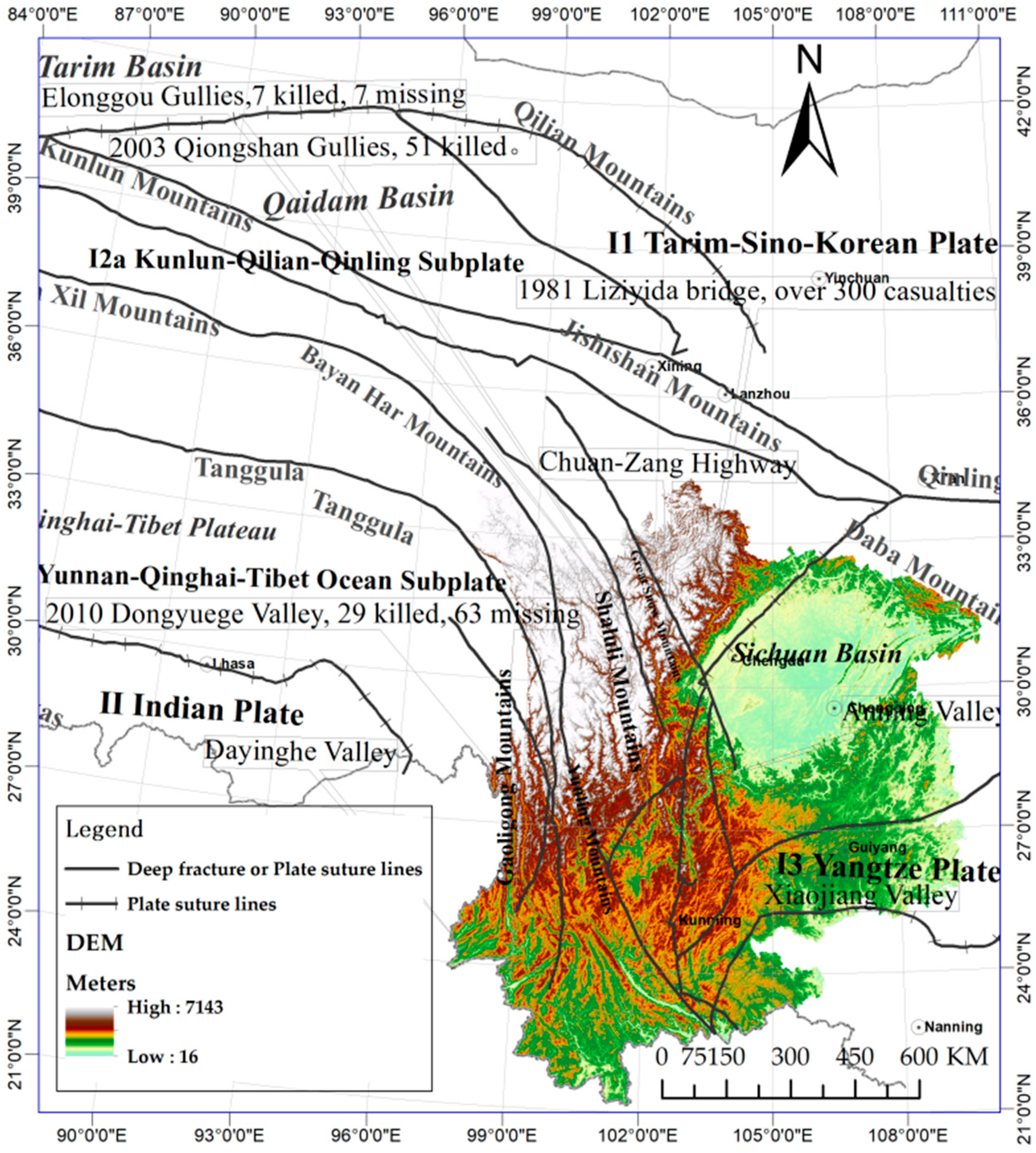
SWC spans an area of approximately 1.14 × 10⁶ km2 and includes Sichuan, Yunnan, Chongqing and Guizhou Provinces according to a comprehensive geographical division of China. This area is located between longitudes 97°28′ E and 110°7′ E and latitudes between 21°18′ N and 34°20′ N (Figure 1), which comprises large terrains that encompass the transitional area between the high Tibetan Plateau and the low alluvial plains. Large differences in neotectonic movements resulted in the creation of diverse topographic forms in this area, including plateaus, high mountains, middle mountains, hills, and basins. The highest point is 7556 m above sea level (a.s.l.) at Gongga Mountain in the northwest, whereas the lowest point is 76.4 m a.s.l. at Hekou County in the southeast. The high relief endows this region’s debris flows with highly dynamic conditions.
This study area is located within the subduction zone between the Eurasian Plate and the Indian Plate (Figure 1). The movements of these continental plates provide this region with a dense distribution of tectonic belts and intense seismic activity, which produces fractured mountain bodies, causes rock debris increase, and supplies the region with abundant debris reserves.
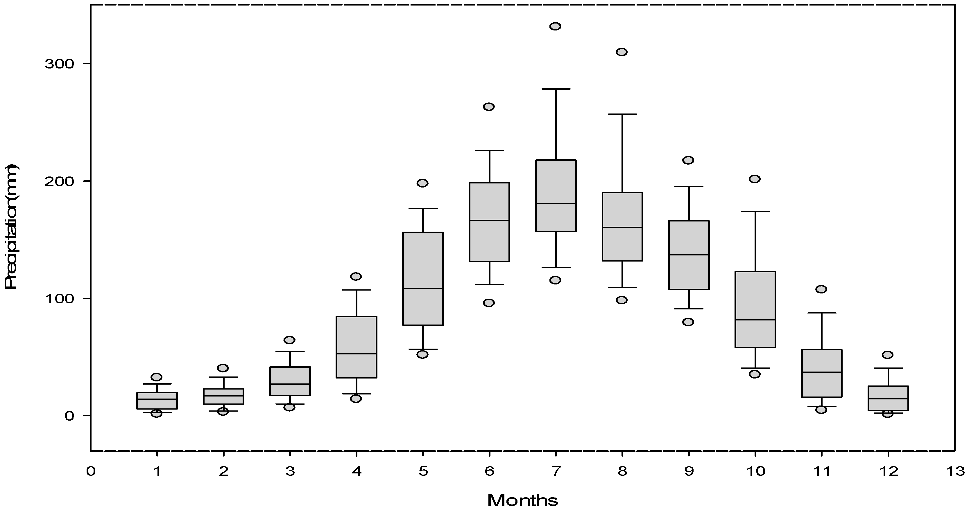
The climate of this area is characterized by subtropical monsoons. Because of series of NS-trending mountains and canyons (Figure 1), monsoons that originate from the Indian Ocean to the southwest and the Pacific Ocean to the southeast can reach far into SWC. The wet, hot monsoons move northward and westward along the canyons, which are prone to forming rainstorms when they are uplifted by mountains. Most locations record an average annual precipitation of 1000–1300 mm, which is mainly concentrated from May to October (Figure 2).
These unique topographic, geomorphic, and meteorological conditions, in addition to the presence of abundant debris, contribute to the high concentration of debris-flow gullies in SWC. The Xiaojiang Valley and Dayinghe Valley in Yunnan Province and the areas along the Anning Valley and Chuan-Zang Highway are all famous around the world for their high-frequency and high-intensity debris flows (Figure 1). Well-developed debris-flow gullies often cause great economic losses and casualties, especially during the storm season from May to August. One such instance occurred in July 1981, when a debris flow washed away the Liziyida Bridge of the Cheng-Kun Railway, causing a train crash with over 300 casualties. The Elonggou Gullies, which are located between Yuezaba and Banong Villages in Yuezha Township, which is located in Danba County in Ganzi, Sichuan Province, experienced a large debris flow on 26 June 2003. Seven people were killed and seven went missing. A debris-flow disaster of similar size occurred in the Qiongshan Gullies in Badi Town on 11 July 2003, in which a village was destroyed completely, and 51 people were killed. On 18 August 2010, a huge debris flow hit Dongyuege in Litoudi Village in Puladi Township, Gongshan County, Nujiang prefecture in Yunnan Province, in which an iron-ore plant was buried, 29 people were killed, and 63 people went missing. Data that were collected from local accounts, news reports and related literature revealed that SWC had experienced 399 debris-flow disasters since 1949, of which nearly 40% were extra-large or large-scale events (i.e., disasters that have killed 10 or more people or caused a loss of more than 5 million Yuan according to the classification criteria from the Ministry of Land and Resources of China). Nearly 1000 deaths from landslides and debris flows are reported each year worldwide [19]. Numerous casualties and economic losses limit socioeconomic development. Therefore, new measures are urgently required to improve disaster prevention and reduce disaster loss.
3. Data and Materials
The data and materials that are analyzed in this paper include debris-flow disaster records, the spatial distributions of debris-flow gullies, and disaster-forming environment and demographic data, which have been comprehensively collected, revised, and corrected from historical records by using GIS tools.
3.1. Records of Debris-Flow Disasters
Records of debris-flow disasters were derived from “Events of debris-flow disasters in China (1949–2008)”, which was published by the Southwest mountainous center of the Data-Sharing Network of Earth System Science (http://www.geodata.cn/). These data were originally collected by the Institute of Mountain Hazards and Environment of the Chinese Academy of Sciences (CAS) in Chengdu, Sichuan Province, from published literature, newspapers, and internet articles. The analyzed events span a range of 60 years from 1949 to 2008. We collated, added and spatially oriented each event again based on the records of SWC-related chronicles and published yearbooks. Three hundred and ninety-nine events were eventually corrected and selected. Data from these events include dates, sites, death tolls, injuries, direct economic losses, and the number of collapsed houses or other buildings. A brief statistical analysis in Table 1 shows that SWC experienced six to seven debris-flow disasters each year from 1949 to 2008, of which 25.4% were extremely large events, 14.6% were large events, 29.9% were medium events, and 34.2% were small events. These disasters caused the deaths of more than 5300 people and a loss of nearly 10 billion Yuan. These data indicate that SWC is the area that is most seriously affected by debris flows in China, with the deaths and direct economic losses in SWC comprising 81.2% and 91.3%, respectively, of those in the entire country.
3.2. Spatial Distribution of Debris-Flow Gullies
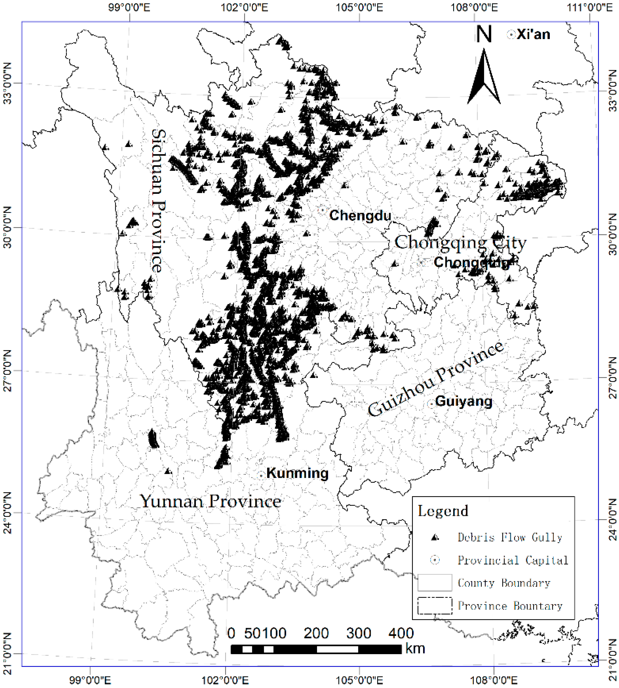
Raw data of the spatial distribution of debris-flow gullies were obtained from surveys of debris flows in China. Three thousand, seven hundred and forty-five gullies were eventually collated; these gullies are mainly situated in counties in central Sichuan Province, northern Yunnan Province and the trans-border areas between Sichuan and Yunnan Provinces (Figure 3). The debris-flow gully density in these regions ranges from a minimum value of 0.24 gully/103 km2 to a maximum value of 24 gullies/103 km2. The data only include limited information regarding positions and do not contain any other characteristics such as drainage areas or length. These data were used to calculate regional debris-flow gully density values, identify the levels of debris-flow hazards and additional environmental factor data to determine debris-flow hazards.
3.3. Disaster-Forming Environmental Data
Disaster-forming environmental data include four categories: geology, topography, meteorology, and human activities. Geological data were digitized from the China Geological Atlas, which was published by the Geological Publishing House in 1996. Factors such as fault density and the distribution and ages of rock strata were extracted, calculated, and used to describe the debris reserve. Topographic data were generated from a Digital Elevation Model (DEM) with a 90 × 90 m resolution. Factors such as slope areas with different degrees, relief, and gully density were from the DEM. Slope areas with different degrees and relief are used to describe the dynamic conditions that formed debris flows. Gully density is used to indicate the breaking conditions of the ground surface. The precipitation from 1951 to 2009 was calculated by using daily records from national meteorological stations in the study area (http://data.cma.cn/). Factors such as the average annual precipitation, monthly variation, and annual number of days with over 25 mm or 50 mm of precipitation were derived and used to describe the water conditions that formed debris flows and their reactivation factors. Human-activity data were processed by using a land-use map with a scale of 1:100,000 and 27 classification types, including cultivated land (8 types), forestland (4 types), grass land (3 types), waters (5 types), urban and rural residential land (2 types), industrial land (1 type), and unused land (4 types) (http://www.resdc.cn). Areas of cultivated land with slopes above 25° were extracted to indicate the influences of human beings on debris flows.
3.4. Demographic Data
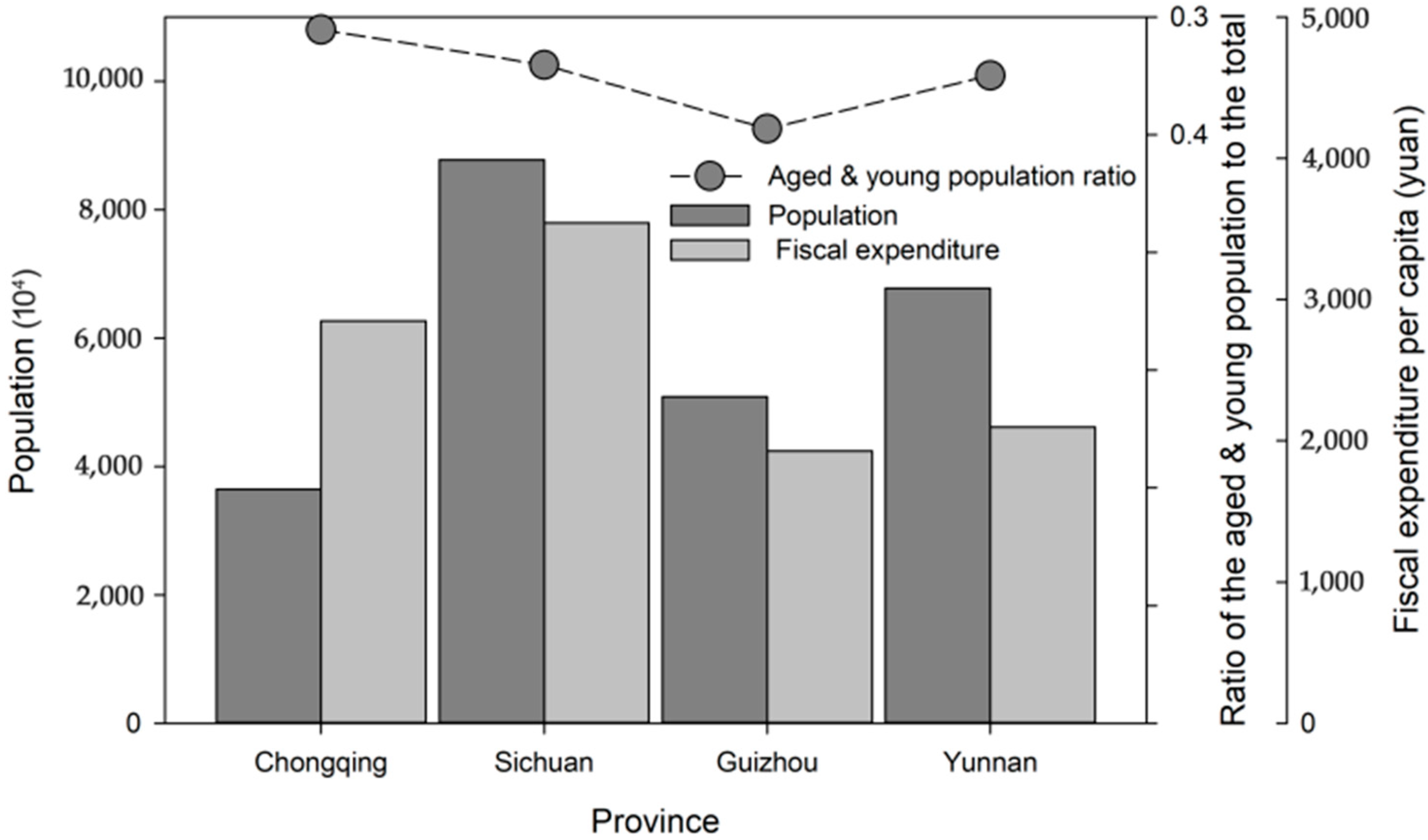
Demographic data that influence vulnerability were collected and calculated from the statistical data of the 2009 yearbooks of provinces such as Sichuan, Yunnan, Guizhou, and Chongqing, alongside the fifth census in China in 2000. These data include the total population, employed and unemployed populations, peasant population, populations of different age groups, number of students in senior high school, fiscal expenditures, GDP, number of beds in hospitals or clinics, etc. A brief statistic shows that Sichuan has the largest population of the four provinces in SWC (Figure 4). The fiscal expenditure per capita in Sichuan province is also the biggest of all, reaching 3543.00 Chinese yuan. Ratio of the population younger than 16 or older than 60 to the total ranges from 0.32 to 0.39. These data were employed to estimate the annual loss of at-risk elements.
4. Methodology
4.1. Risk Estimation Model
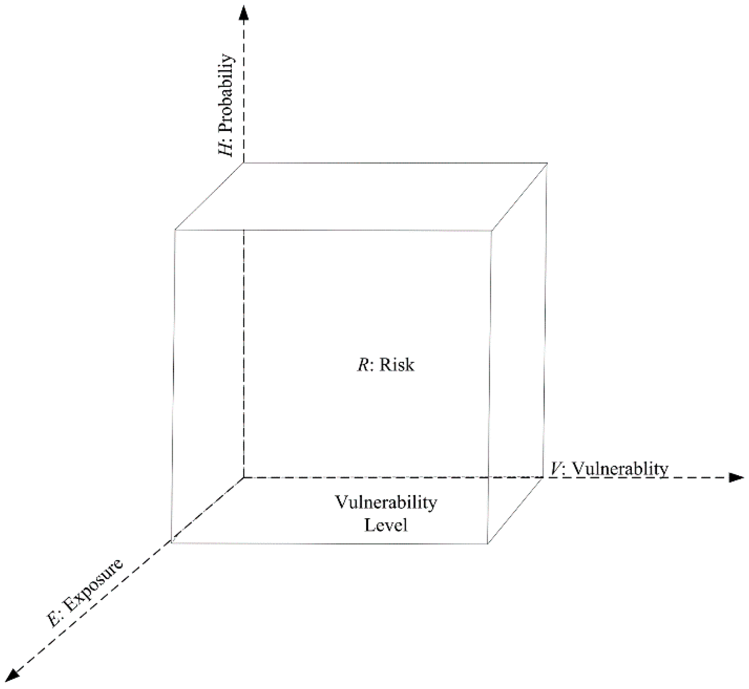
The investigation of debris-flow risk in this paper involves two steps: a hazard assessment and a vulnerability assessment. Three factors are involved in this method, namely, the occurrence probability of debris flows, the vulnerability of an at-risk element and its exposure. We can use the volume of a cuboid to represent the method (Figure 5), in which the rectangular height represents the disaster hazard which varies with the probability and intensity of a specific debris flow; the basal area, which is calculated from the vulnerability and exposure (represented as the width and length, respectively, in Figure 5), expresses the level of vulnerability. According to Figure 5, the following formula was used in our investigations [20,21,22,23]
where Rij (risk) refers to the risk of the i-th at-risk element i from the j-th scale of debris flows; Pj (probability) is the probability or frequency of the j-th scale of debris flows; Vij (vulnerability) is the vulnerability (or fragility rate) of the i-th at-risk element from the j-th scale of debris flows; Ei (exposure) is the amount of exposure of the i-th at-risk element that is influenced by debris flows; i = 1, 2, …, n, where n is the number of types of at-risk elements; and j = 1, 2, …, m, where m is the classification of scales or intensities of disasters.
4.2. Hazard Evaluation Method
Debris-flow disaster events are used in view of the hazard varying with the probability or intensity of debris flows. There are only 399 debris-flow disaster events collected. They might be not enough to calculate probability or intensity of debris flows in SWC directly. Thus an analogy-deductive method combined with an intensity-frequency analysis was purposed to evaluate debris-flow hazards in this study. First, a similarity model was chosen from our previous research [15] to divide the study area into different types of hazard zones. Then, an intensity–frequency analysis from the disaster events was calculated in each type of hazard zones to perform a quantitative assessment.
4.2.1. Factors for Debris-Flow Hazard Zoning
Debris-flow hazard zoning is carried out based on the similarity model with factors that influencing debris hazard indirectly. The similarity-based debris flow hazard model can evaluate regional debris hazard level with the similarity vectors and the hazard levels of standard hazard-level-type regions (HLTR). The steps include determining HLTR, selecting suitable hazard-influencing factors, calculating similarities between the factors of the assessment-pending regions (APR) and those of HLTR, and assessing hazard-level types of APR [15]. This study first chose debris-flow gully density as the criterion to classify HLTR in SWC. Seventy-four counties with debris-flow gully data were thus classified into four HLTRs. The debris-flow gully distributions in each type of HLTR are shown in Table 2. Seven indicators were then selected according to their gray correlation degrees associated with debris-flow gully density in the HLTRs. These factors include the fault density, area percentage of sloping land between 10° and 25°, number of days with precipitation ≥25 mm, monthly precipitation variation, weathering coefficient of rocks, gully density and area percentage of sloped cultivated land ≥25° (Table 3).
4.2.2. Intensity–Frequency Calculation
The hazard-level types of APRs are quantitatively determined with debris-flow frequency of different intensities, which is calculated by using Equation (2)
where Pij is the annual frequency of j-th-level disasters in the i-th evaluation unit; Nij is the number of j-th-level disaster events in the i-th evaluation unit; X is an event or a debris-flow disaster with a higher scale than XT, which is the representative disaster sample according to the classification; and T is the return period of event X beyond event XT in years.
4.3. Vulnerability Evaluation Model
Quantitative approaches for evaluating vulnerability need to be complemented with qualitative approaches considering the full complexity. High vulnerability is an outcome of skewed development processes such as environmental mismanagement, demographic changes, rapid and unplanned urbanization, and the scarcity of livelihood options for the poor [7]. Physical, social, economic, and demographic factors were selected from the literature in this study to qualitatively measure the vulnerability based on the definition of vulnerability from the United Nations International Strategy for Disaster Reduction [25]. Different vulnerability zones were classified according to these factors, and then the fragility rate in each type of zones was analyzed to receive a quantitative result. Therefore, this section includes three models: a vulnerability zoning model, an exposure calculation model, and a fragility-rate statistical model.
4.3.1. Vulnerability Zoning Model
Because of its complexity, vulnerability zoning is often indirectly performed by using a set of indicators such as the population density, popularized rate of senior high school education, per capita income, GDP, and urbanization rate [26,27]. Cutter et al. selected 11 independent composite factors from 42 variables to construct a social vulnerable index (SoVI) with the purpose to assess environmental hazards in USA. The variables involved socioeconomic status (income, political power, and prestige), gender, race and ethnicity, age, commercial and industrial development, employment loss, rural or urban setting, residential property, infrastructure and lifelines, renters, occupation, family structure, education, population growth, medical services, social dependence and special needs populations [28]. Huang et al. introduced a DEA model to assess province-level vulnerability in China. These authors used factors that cover the danger index of regional hazards (DI), exposure of regional socioeconomic systems (EI) and regional natural disaster losses (LI), which included 24 variables [29]. Seventeen factors were employed in this paper, which are related to the economy, society and natural processes, to assess population vulnerability based on the above studies [25,28,29]. These variables are:
- (1)
- Social and economic factors that affect population vulnerability: population (X1), population density (X2), fiscal expenditure per capita (X3), GDP per capita (X5), ratio of the employed population in a rural area to the total population (X6), ratio of the peasant population to the total population (X7), popularized rate of senior high school education (X8), ratio of the population younger than 16 or older than 60 to the total population (X9), urbanization rate (X10), and numbers of beds in hospitals or clinics (X11).
- (2)
- Environmental factors for population vulnerability: annual precipitation (X15), monthly precipitation variation coefficient (X16), number of days with precipitation ≥25 mm (X17), area percentage of land with slopes ≥25° (X18), gully density (X19), and area percentage of cultivated land with slopes ≥25° (X20).
- (3)
- Debris-flow hazard (X21), which is obtained from the results in Section 4.2.
Studies showed that the relationship between the factors and population vulnerability is complex and complicated [27,28]. Factors such as population density positively affect the vulnerability of at-risk elements, while the popularized rate of senior high school education is negatively related to vulnerability. Many other indicators exist whose effects on at-risk elements cannot be expressed by a simple linear relationship. One investigation showed that per capita incomes and disaster risk appear to be correlated by curved lines [30]. Disaster loss increases with per capita income when the per capita GDP is $5044, $3360, or $4688 and then begins to decline. In addition, some indicators in the literature, such as fiscal expenditure per capita and GDP per capita, recorded correlations between themselves. Therefore, this paper utilized the factor analysis method to zone the vulnerability in SWC.
The factor analysis method was first proposed by C. Spearman in 1904 and has been implemented in several statistical analysis programs, such as solutions statistical package for the social sciences (SPSS), since the 1980s. This method is primarily used to remove redundant or highly correlated variables with several independent common factors. A common factor is a linear combination of original variables. The factor analysis method will find the first common factor that accounts for as much variation in the original variables as possible. After the first, another common factor that accounts for as much of the remaining variation as possible and is uncorrelated with the previous common factor will be calculated. The method continues in this way until there are as many common factors as original variables. These common factors can be used to replace the original variables. This method can thereby yield comprehensive and scientific results by integrate variables with complex relationships into several new independent common factors [31].
4.3.2. Exposure Calculation Model
Exposure refers to the populations in areas that are affected by debris flows. If these populations are evenly distributed in an evaluation unit, their exposure can be calculated by using Equation (3) in a GIS environment according to debris flow spatial distribution and census data
where Ei is the exposure of i at-risk elements, Ci is the total amount of i at-risk elements in an evaluation unit, and r is the ratio of the area of the debris-flow to that of the total evaluation unit.
4.3.3. Fragility-Rate Statistical Model
According to the official definition [7], population vulnerability refers to the ratio of casualties (e.g., deaths, disappearances, injuries) to the total exposed population during a disaster. Vulnerability is indicated by fragility rates in this paper, i.e., the expected loss that is caused by disasters of the same scale. The fragility rate is calculated from Equation (4) by using a similar inference method from historical data
where Vij is the fragility rate of the i-th at-risk element when facing debris-flow disasters of the j-th intensity or scale; Lr is the loss rate of the i-th at-risk element from a debris-flow disaster of the j-th intensity; Lij is the loss amount of the i-th at-risk element from a debris-flow disaster of the j-th intensity; Ei is the exposure of the i-th at-risk element; pij is the probability of Lij for the i-th at-risk element when experiencing debris-flow disasters of the j-th intensity; and i and j are the same as in Equation (1).
5. Results and Discussion
5.1. Hazard Evaluation
5.1.1. Hazard Zoning
The debris-flow hazard zoning in SWC was determined by HLTRs and the selected factors in Section 4.2.1 by using a similarity-based assessment model. The results are shown in Figure 6.
Figure 6 shows that high-density debris-flow zones (III- and IV-type zones) are located in mountainous areas that surround the Sichuan Basin, the bordering strip between Sichuan and Yunnan Provinces, northern and eastern Yunnan Province, and eastern Guizhou Province. Counties such as Jinghong and Xichang have very similar debris-flow gully densities as those in the IV-type standard HTLRs. Cracked surface, high relief and concentrated abundant precipitation in these areas are conducive to the development of debris flows [9,32]. According to the selected indicators, these areas should belong to the highest-level debris-flow hazard zone. However, disasters are natural and variable processes that can pose a detrimental effect to human existence or activity. These events are characterized by natural and human properties. Therefore, the occurrence probability in each type of hazardous zone was further estimated by using historical disaster records to more scientifically determine their hazard levels.
5.1.2. Frequency Calculation
The frequencies of debris-flow disasters were calculated from the events of debris-flow disasters in China (1949–2008), which were introduced in Section 3, by using the method in Section 4.2. The annual frequencies of debris-flow disasters in the I~IV types of hazardous zones are listed in Table 4.
Table 4 shows that the III-type zones are extremely high hazard zones. In these areas, small debris-flow disasters occurred every 0.71 years, medium-sized disasters occurred more than once every two years and extremely large disasters occurred every three years. The hazard aggregative index reached 46.59. The II-type zones are characterized as high-level hazard zones and have an annual frequency of extremely large debris-flow disasters of 0.11. The IV and I type of hazardous zones are moderate- and low-level hazard zones, respectively. The hazard levels of the IV-type hazardous areas are lower than those in the II- and III-level zones but have denser debris-flow gullies. This phenomenon was caused by their rugged environmental conditions, which result in low populations. Another reason may be that the people who live in these areas have implemented appropriate disaster-risk management in some locations that are susceptible to debris flows, thus resulting in fewer records.
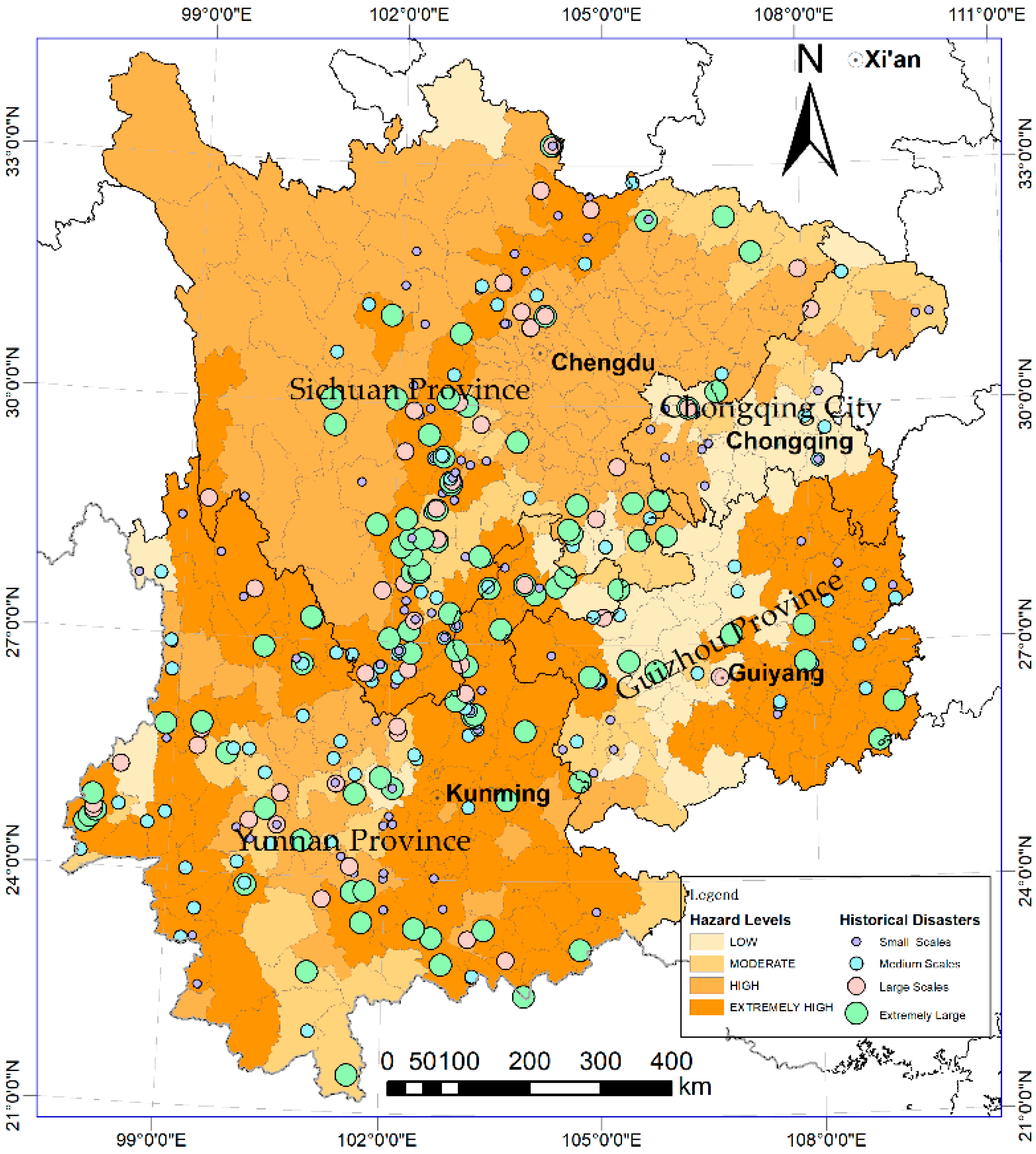
These results can be verified by analyzing the distribution of debris-flow disaster records in Figure 7, which shows that disaster records (especially on large and extremely large scales) are far more likely to be found in extremely high hazard zones. These results have some practical significance. The spatial distributions of debris-flow disaster hazards can also be found in Figure 7, in which the most hazardous locations are the central strip that extends from Qingchuan in the north to Huili in the south, the bordering area between Sichuan and Yunnan, the western and southeastern regions of Yunnan, and the eastern half of Guizhou. Counties in most of Chongqing, the central area of Guizhou and Yunnan, are characterized by low or moderate hazard zones.
5.2. Vulnerability Estimation
5.2.1. Vulnerability Zoning
The selected factors in Section 4.3.1 were analyzed with solutions statistical package for the social sciences (SPSS) based on the methods above. Data verification yielded a KMO (Kaiser–Meyer–Olkim) value of 0.827, indicating that these factors are suited for factor analysis. Five common factors with eigenvalues over 1 were selected, with the cumulative variance contribution ratio reaching 74.009%. The common factor F1 was named as a social-development level because this factor had a higher factor loading in X8, X10, X11, and X5. F2 was chosen as a meteorological factor because of its higher loading in X15 and X17. F3 was chosen as a disaster-resistance factor because of its higher loading in X3. F4 was chosen as a debris-flow hazard factor because of its higher loading in X20 and X21. F5 was chosen as a topographic factor because of its higher loading in X19 (Table 5). These five common factors, which cover the categories of meteorology, debris-flow hazard, social development, disaster resistance and topography, were then integrated to determine the vulnerability zones in SWC.
A many-to-many regression analysis (i.e., least-squares estimation) was used to estimate the score function for each common factor. Their coefficient matrices are listed in Table 6.
Composite scores were calculated from Formula (5) as
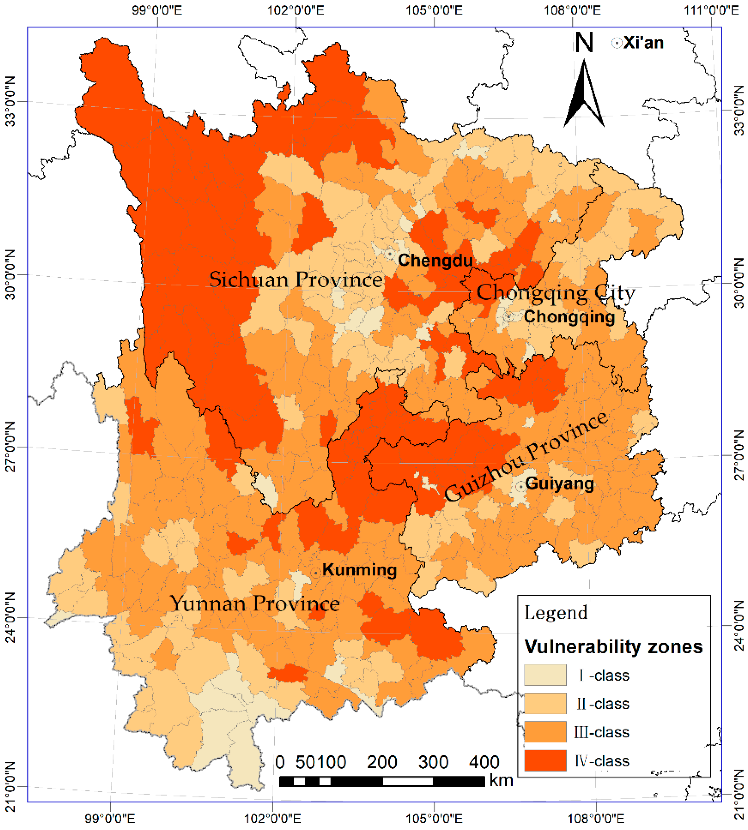
where λi is the factor loadings of the common factors. The population vulnerability in SWC was classified into four types with equal intervals based on the composite scores. The results were mapped and shown in Figure 8.
Figure 8 shows that the I-class vulnerability zones are located in more than 40 counties, such as Mengla, Jinghong, Cuiyun, and Jiangcheng in southern Yunnan and Yuzhong, Chengdu, Jiangbei, Leshan, and Ya’an in the Sichuan Basin. The II-class vulnerability zones are located in the annular regions near the I-class zones, including counties such as Menghai, Menglian, Lancang, and Pu’er in southwestern Yunnan, counties around the Sichuan Basin, and Anshun, Pu’an, and Xingyi in Guizhou. The III-class vulnerability zones are mainly distributed in the central-western region of Yunnan Province, the eastern and northern regions of Guizhou Province, central Chongqing, and the bordering counties among Guizhou, Sichuan, and Yunnan, which span nearly 200 counties. The IV-class vulnerability zones are located in counties in the western and northwestern regions of Sichuan and Zhaotong in Yunnan Province and Bijie in Guizhou Province. This classification ensures that counties of the same type have the most similar features when encountering debris flows. These zones were compared and validated with the historical disaster records, as discussed below.
5.2.2. Fragility Rate Calculation
The ratio of disaster loss to total exposure, i.e., the loss rate of debris-flows of different scales in all classes of vulnerability zones, can be calculated from debris-flow records from 1949 to 2008. One hundred and eighty-nine records of debris flows with casualties were used and visualized to validate the above results (Figure 9).
Eleven records of debris-flow disasters were found in the I-class vulnerability zone (Figure 9). The loss rates (i.e., the ratio of the death toll in a disaster to the total population that was exposed) range from 0.07 to 2.70 persons for every 10 thousand people. A total of 52 records were discovered in the II-class zone, with loss rates ranging from 0.01 to 13.16 persons per 10 thousand people. A total of 94 records were found in the III-class zone, with a minimum loss rate of 0.01 persons per 10 thousand people and a maximum of 8.64 persons per 10 thousand people. A total of 32 records were found in the IV-class zone, with loss rates ranging from 0.01 to 14.67 persons per 10 thousand people. These results demonstrate that more debris-flow disasters are found in III-class and II-class zones than in other zones. Therefore, it is not rigorous to say that the vulnerability level generally increases from the I-class to IV-class zones. The damage-scale curves in Figure 9 yield similar conclusions. The highest R2 value in the I-class zone is only 0.46. The values of the other zones are all lower than 0.4, which reflect much lower reliability. These values fail to directly explain the vulnerability levels. Therefore, fragility rates—i.e., the rates of expected loss, were calculated instead to reflect the vulnerability levels of each zone—which were estimated by using Equation (5) in Section 4.3.3 and are listed in Table 7.
Table 7 indicates that the IV-class zones are extremely high vulnerability zones. Their fragility rate reaches 3.89 persons per 10 thousand people, and their records show that the largest debris-flow disaster could cause as many as 14 casualties per 10 thousand people. The II-class zones are high-level zones. Their population fragility rate is 3.77 persons per 10 thousand people. The III-class zones are medium-level zones and the I-class zones are low-level zones. Their fragility rates are 2.69 and 1.49 persons per 10 thousand people, respectively.
5.3. Risk Estimation
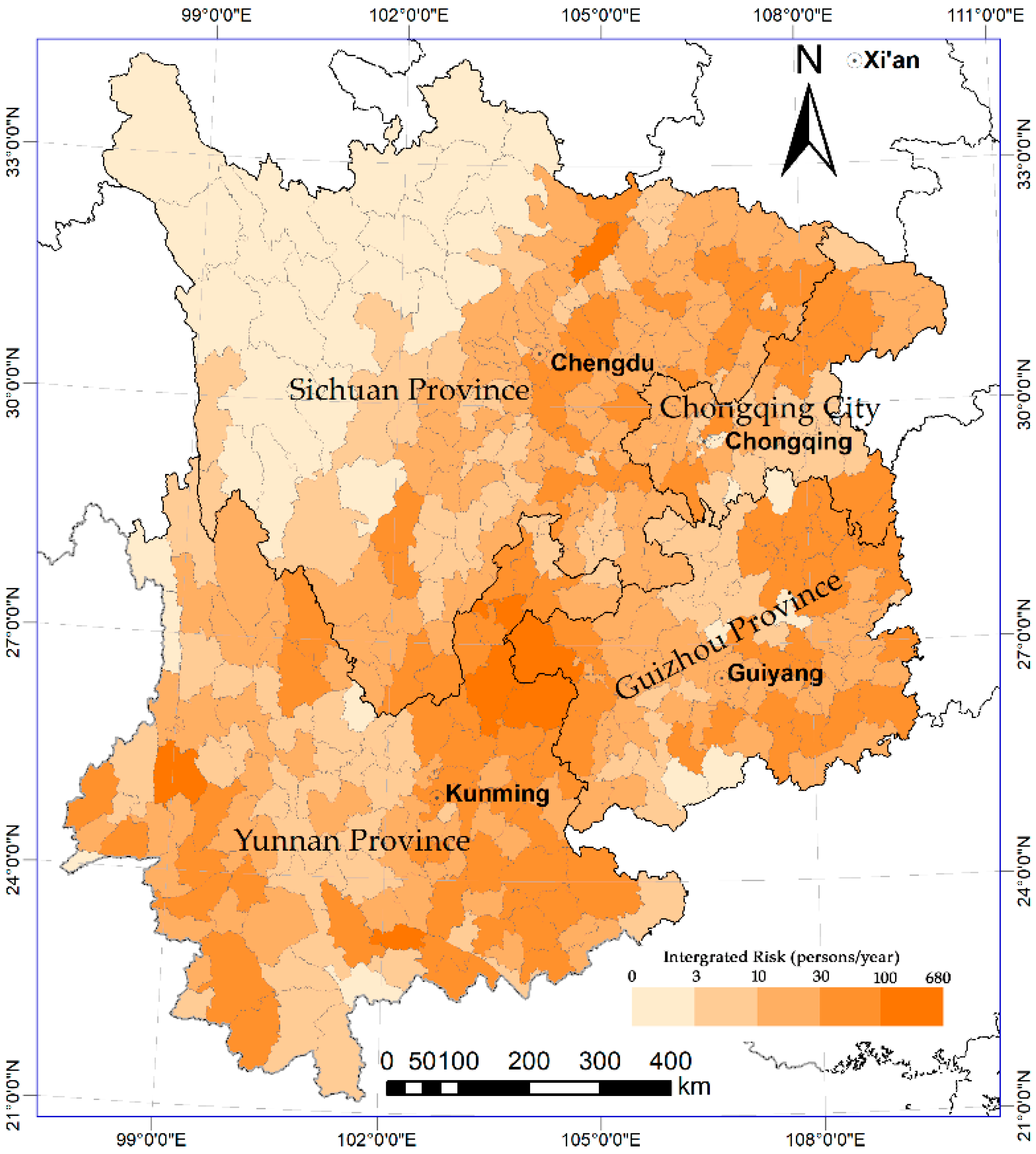
Risk was estimated by using Equation (1) in Section 4. Pj in Equation (1) is from the frequency of each hazard type in Section 5.1.2. In this paper, this value is expressed in units of events/year. Vij was obtained from the fragility rates in Section 5.2 and is expressed in units of persons per 10 thousand people. The exposure (Ei) in counties was calculated from demographic data from 2008. For example, Zhaotong is classified as a III-type debris hazard zone and a IV-class vulnerability zone. This area’s population risk of extremely large disasters was calculated with a frequency of 0.36 event/year, a fragility rate of 2.25 persons per 10 thousand people, and a total exposure of 5,295,000 persons. This area’s casualty risk from extremely large disasters is 429 persons, whereas that from large disasters is 52 persons, that from medium disasters is 110 persons, and that from small disasters is 87 persons. These results can then be integrated into one comprehensive risk of 678 persons. Comprehensive risk values were calculated from different scales of debris-flow disasters in each county in this way and are shown in Figure 10.
Figure 10 shows that this risk gradually increases from the southeastern region of the study area and reaches a maximum value of over 100 persons/year at the Jiangyou–Zhaotong–Baoshan Line before decreasing to the northwest. Of the 4 provinces, Yunnan is characterized by its extremely high risk: 34.4% of its counties (43 of a total 125) have a risk of over 30 persons/year. The risk in Zhaotong and Honghe reaches over 500 persons/year, and the total risk in the entire province reaches 4578 persons/year. Sichuan Province is characterized by high risk, with a total risk of 2800 persons/year. Of the 161 counties that were studied here, nearly one-fifth of these counties yielded a risk of more than 30 people; these counties are scattered in the Sichuan Basin and the border area between Yunnan and Sichuan. Guizhou Province has a moderate risk: counties in its eastern and southeastern region and in the boundary area between Guizhou and Yunnan have a risk of more than 30 persons. Chongqing City is characterized by low risk.
5.4. Discussion
The comprehensive risk-analysis methodology in this paper integrated models from hazard and vulnerability studies. Hazard and vulnerability zoning were indirectly implemented by using variables from the literature. These variables were selected from references [15,28,29], but some differences existed in terms of the unique geological, geomorphological, meteorological, social, and economic conditions in SWC. Liu et al. (2013) found that the rock conditions that form debris flows (in terms of geology) and mean annual precipitation (in terms of meteorology) are closely related to debris-flow gully density [15]; instead of these variables, this research used the fault density and number of days with precipitation ≥25 mm because the latter yielded higher correlation scores in this investigation. Cutter et al. (2003) considered race and ethnicity in their SoVI calculations, while no such issue currently exists in China [28]. Huang et al. (2013) added natural-disaster losses to their vulnerability assessment [29]. The results of this research indicated that vulnerability is an intrinsic characteristic of at-risk elements [27] and that disaster losses result from both hazard and vulnerability. Therefore, disaster records were used to explore vulnerability levels after determining the zoning in this paper. In this assessment, entire populations of counties were used to calculate exposure because of limited data, which can increase risk levels. These changes and issues should be further explored in future studies.
Although risk assessment that is based on these variables cannot entirely avoid these disastrous natural phenomena [32], risk analysis can be useful in preparing for disasters and informing endangered communities and the general public [4], which can in turn assist policy makers in taking mitigation measures to decrease risk. The results of the hazard and vulnerability zoning and risk calculation in this paper could thus provide necessary information to regional risk-management communities and endangered counties.
6. Conclusions
In this study, a comprehensive evaluation of population risk from debris flow disasters in SWC was performed by using a method that was based on a model from UNISDR and the results of related studies. The main steps of this model include the determination of debris-flow disaster-hazard zoning, estimation of the annual frequency of different scales of the disaster, identification of factors that affect population vulnerability zoning, and calculation of fragility rates. The population risk was calculated for each scale of debris-flow disasters and then integrated together. The conclusions of this study are:
- (1)
- Debris flows are mainly spread across the mountainous areas around the Sichuan Basin, the border area between Sichuan and Yunnan, eastern and southern Yunnan Province, and eastern Guizhou Province. More than 200 counties were classified as extremely high- or high-density areas of debris-flow gullies, which cover an area of 580,000 km2 and contain a population of 89.97 million people. An analysis of historical records showed that the hazard level is not exactly consistent with the regional debris-flow gully density. The hazard level is highest in the high-density counties and not in the extremely high-density areas; in the high-density areas, the annual frequency of extremely large-scale debris flows reaches 0.36 and small- and medium-scale events occur almost every year.
- (2)
- The vulnerability of the at-risk population was assessed with a factor analysis model. The results showed that extremely highly vulnerable zones are distributed in 79 counties, including counties to the west and southwest of Sichuan Province, Zhaotong in Yunnan Province, and Bijie in Guizhou Province, which cover an area of approximately 349,000 km2 and have a population of 55,350,000. Their comprehensive fragility rate is 3.89 persons per 10,000 people. In some cases, extremely large debris-flow disasters could result in 14 casualties per 10,000 exposed people. The highly vulnerable zones include 111 counties around the Sichuan Basin, southwestern Yunnan Province and the central and southern regions of Guizhou Province. This area spans 264,000 km2 and contains a population of approximately 48,960,000 people. The comprehensive fragility rate is 3.77 persons per 10,000 people, which is slightly less than that of the extremely high vulnerability zone.
- (3)
- Comprehensive population risk gradually increases from the southeastern region to the central region of SWC, reaches its highest on the Jiangyou–Zhaotong–Baoshan Line, and then gradually reduces to its lowest in the northwestern region. Specifically, the extremely high-risk counties with extremely large-scale disasters include Zhaotong, Honghe, Baoshan, and Xuanwei in Yunnan Province and Weining in Guizhou Province. These regions are scattered throughout the central region of SWC, with population risks of up to 100 persons/year. The counties around the extremely high-risk zones—such as Wanzhou, Youyang, Xiushan, Yunyang, and Jiangjin in Chongqing City, Huize and Guangnan in Yunnan Province, Jiaoyou and Xichang in Sichuan Province, and Shuicheng and Hezhang in Guizhou Province—are characterized by a high annual frequency of debris-flow disasters. Their population risk is over 30 persons/year.
Author Contributions
G.L. and X.X. conceived and designed the investigation; E.D. and W.W. analyzed the data and contributed materials; G.L. and A.X. wrote the paper.
Funding
The work is funded by the Natural Science Foundation of China (NSFC) under Grant No. 41561020, the National Basic Research Program of China (973 Program) under Grant No. 2012CB955403 and subject selection of scientific research projects of Gannan Normal University.
Conflicts of Interest
The authors declare no conflict of interest. The founding sponsors had no role in the design of the study; in the collection, analyses, or interpretation of data; in the writing of the manuscript, or in the decision to publish the results.
References
- Iverson, R.M. Debris flows: Behaviour and hazard assessment. Geol. Today 2014, 30, 15–20. [Google Scholar] [CrossRef]
- Santi, P.; Hewitt, K.; VanDine, D.; Cruz, E.B. Debris-flow impact, vulnerability, and response. Nat. Hazards 2011, 56, 371–402. [Google Scholar] [CrossRef]
- Takahashi, T. Debris Flow: Mechanics, Prediction and Countermeasures; CRC Press: Boca Raton, FL, USA, 2014. [Google Scholar]
- Glade, T. Linking debris-flow hazard assessments with geomorphology. Geomorphology 2005, 66, 189–213. [Google Scholar] [CrossRef]
- Dieter, R. Debris-flow hazard assessment and methods applied in engineering practice. Int. J. Eros. Control Eng. 2016, 9, 81–90. [Google Scholar]
- He, Y.P.; Xie, H.; Cui, P.; Wei, F.Q.; Zhong, D.L.; Gardner, J.S. GIS-based hazard mapping and zonation of debris flows in xiaojiang basin, Southwestern China. Environ. Geol. 2003, 45, 286–293. [Google Scholar] [CrossRef]
- Cardona, O.-D.; van Aalst, M.K.; Birkmann, J.; Fordham, M.; McGregor, G.; Mechler, R. Determinants of risk: Exposure and vulnerability. In Managing the Risks of Extreme Events and Disasters to Advance Climate Change Adaptation; Field, C.B., Barros, V., Stocker, T.F., Qin, D., Dokken, D.J., Ebi, K.L., Mastrandrea, M.D., Mach, K.J., Plattner, G.-K., Allen, S.K., et al., Eds.; Cambridge University Press: Cambridge, UK; New York, NY, USA, 2012; pp. 65–108. [Google Scholar]
- Alexander, D. Natural disasters: A framework for research and teaching. Disasters 1991, 15, 209–226. [Google Scholar] [CrossRef] [PubMed]
- Xu, W.; Jing, S.; Yu, W.; Wang, Z.; Zhang, G.; Huang, J. A comparison between bayes discriminant analysis and logistic regression for prediction of debris flow in Southwest Sichuan, China. Geomorphology 2013, 201, 45–51. [Google Scholar] [CrossRef]
- Jeffers, J.M. Integrating vulnerability analysis and risk assessment in flood loss mitigation: An evaluation of barriers and challenges based on evidence from Ireland. Appl. Geogr. 2013, 2013, 44–51. [Google Scholar] [CrossRef]
- Liang, W.; Zhuang, D.; Jiang, D.; Pan, J.; Ren, H. Assessment of debris flow hazards using a bayesian network. Geomorphology 2012, 171, 94–100. [Google Scholar] [CrossRef]
- Tsao, T.C.; Hsu, W.K.; Cheng, C.T.; Lo, W.C.; Chen, C.Y.; Chang, Y.L.; Ju, J.P. A preliminary study of debris flow risk estimation and management in Taiwan. In Proceedings of the Interpraevent 2010—International Symposium in Pacific Rim, Taibei, Taiwan, 26–30 April 2010; pp. 930–939. [Google Scholar]
- Calvo, B.; Savi, F. A real-world application of Monte Carlo procedure for debris flow risk assessment. Comput. Geosci. 2009, 35, 967–977. [Google Scholar] [CrossRef]
- Stancanelli, L.M.; Peres, D.J.; Cancelliere, A.; Foti, E. A combined triggering-propagation modeling approach for the assessment of rainfall induced debris flow susceptibility. J. Hydrol. 2017, 550, 130–143. [Google Scholar] [CrossRef]
- Liu, G.; Dai, E.; Ge, Q.; Wu, W.; Xu, X. A similarity-based quantitative model for assessing regional debris-flow hazard. Nat. Hazards 2013, 69, 295–310. [Google Scholar] [CrossRef]
- Procter, E.; Bollschweiler, M.; Stoffel, M.; Neumann, M. A regional reconstruction of debris-flow activity in the Northern Calcareous Alps, Austria. Geomorphology 2011, 132, 41–50. [Google Scholar] [CrossRef]
- Kappes, M.; Malet, J.-P.; Remaître, A.; Horton, P.; Jaboyedoff, M.; Bell, R. Assessment of debris-flow susceptibility at medium-scale in the Barcelonnette basin, France. Nat. Hazards Earth Syst. Sci. 2011, 11, 627–641. [Google Scholar] [CrossRef]
- Yang, Z. Relationship between geomorphology and plate tectonics movement in Southwest China. J. Southwest China Norm. Univ. (Nat. Sci. Ed.) 1982, 4, 34–40. [Google Scholar]
- Dilley, M.; Chen, R.S.; Deichmann, U. Natural Disaster Hotspots: A Global RISK Analysis; Hazard Management Unit, World Bank: Washington, DC, USA, 2005; pp. 1–132. [Google Scholar]
- Fell, R.; Corominas, J.; Bonnard, C.; Cascini, L.; Leroi, E.; Savage, W.Z. Guidelines for landslide susceptibility, hazard and risk zoning for land use planning. Eng. Geol. 2008, 102, 85–98. [Google Scholar] [CrossRef] [Green Version]
- IUGS Working Group on Landslides, Committee on Risk Assessment. Quantitative risk assessment for slopes and landslides: State of the art. In Proceedings of the International Workshop on Landslides Risk Assessment, Honolulu, HI, USA, 19–21 February 1997; Cruduen, D.M., Fell, R., Eds.; Balkema: Rotterdam, The Netherlands, 1997; pp. 3–12. [Google Scholar]
- Gentile, F.; Bisantino, T.; Trisorio, L.G. Debris-flow risk analysis in south Gargano watersheds (Southern-Italy). Nat. Hazards 2008, 44, 1–17. [Google Scholar] [CrossRef]
- UNISDR. Terminology of Disaster Risk Reduction. Available online: http://www.unisdr.org/eng/library/lib-terminology-eng%20home.htm (accessed on 12 November 2012).
- Chan, J.; Tong, T. Multi-criteria material selections and end-of-life product strategy: Gray relational analysis approach. Mater. Des. 2007, 28, 1539–1546. [Google Scholar] [CrossRef]
- UNISDR. 2009 UNISDR Terminology on Disaster Risk Reduction. Available online: http://www.unisdr.org/we/inform/publications/7817 (accessed on 18 June 2017).
- Cutter, S.L.; Mitchell, J.T.; Scott, M.S. Revealing the vulnerability of people and places: A case study of Georgetown County, South Carolina. Ann. Assoc. Am. Geogr. 2004, 90, 713–737. [Google Scholar] [CrossRef]
- Du, X.; Lin, X. Conceptual model on regional natural disaster risk assessment. Procedia Eng. 2012, 45, 96–100. [Google Scholar] [CrossRef]
- Cutter, S.L.; Boruff, B.J.; Shirley, W.L. Social vulnerability to environmental hazards. Soc. Sci. Q. 2003, 84, 242–261. [Google Scholar] [CrossRef]
- Huang, J.; Liu, Y.; Ma, L.; Su, F. Methodology for the assessment and classification of regional vulnerability to natural hazards in China: The application of a DEA model. Nat. Hazards 2013, 2013, 115–134. [Google Scholar] [CrossRef]
- Kellenberg, D.K.; Mobarak, A.M. Does rising income increase or decrease damage risk from natural disasters? J. Urban Econ. 2008, 63, 788–802. [Google Scholar] [CrossRef]
- Bartholomew, D.; Steele, F.; Galbraith, J.; Moustaki, I. Analysis of Multivariate Social Science Data; Taylor & Francis: Abingdon, UK, 2008. [Google Scholar]
- Di, B.F.; Chen, N.S.; Cui, P.; Li, Z.L.; He, Y.P.; Gao, Y.C. GIS-based risk analysis of debris flow: An application in Sichuan, Southwest China. Int. J. Sediment Res. 2008, 23, 138–148. [Google Scholar] [CrossRef]
Figure 1.
Plate tectonics in Southwest China. The geomorphology and plate tectonics are revised from the reference [18]. The DEM data are provided by International Scientific & Technical Data Mirror Site, Computer Network Information Center, Chinese Academy of Sciences. The map coordinates are in the Krasovsky_1940 reference system with Albers projection.

Figure 2.
Average monthly precipitation in SWC. The dots show the 5th (lower)/95th (upper) percentiles of monthly precipitation from 1951 to 2009. The short-horizontal lines represent the 90th percentiles, 75th percentiles, medians, 25th percentiles, and 10th percentiles respectively from the top to the bottom of the box symbol.

Figure 3.
Map of debris flow distribution in SWC China.

Figure 4.
Demographic statistic in provinces in SWC.

Figure 5.
Conceptual model of debris flow risk China.

Figure 6.
Map of debris flow hazard zones in SWC. The hazard zones of Types I to IV are determined with their highest similarity to the standard HLTRs in Table 2.
Figure 6.
Map of debris flow hazard zones in SWC. The hazard zones of Types I to IV are determined with their highest similarity to the standard HLTRs in Table 2.

Figure 7.
Hazard-levels of debris-flow disasters in counties in SWC. The hazard levels are determined with the frequency of debris flow disasters in Table 4, where the III-type hazard zones are characterized with extremely high level hazard; the II-type belongs to the high level, the IV-type the moderate level, and the I-type the low level. The historical disasters are from the records of debris-flow disasters which are illustrated in Section 3.1.

Figure 8.
Vulnerability zoning for debris-flow disaster in SWC. The four vulnerability zones are classified according to the result of the factor analysis method. These classification shows the most similar vulnerability in the same class zones and the biggest difference between different classes.
Figure 8.
Vulnerability zoning for debris-flow disaster in SWC. The four vulnerability zones are classified according to the result of the factor analysis method. These classification shows the most similar vulnerability in the same class zones and the biggest difference between different classes.

Figure 9.
Scatter plots of population loss rate from records in each class of vulnerability zone in SWC. The horizontal axis represents scales of debris flow disaster. 1~4 represent small, medium, large, and extra-large disaster respectively. This classification is according to the same criteria presented in Table 1. The disaster records are introduced in Section 3.1.

Figure 10.
Integrated population risk from debris flow disasters. The unit is persons/year (persons/yr). The integrated risk is calculated with Equation (1). The probability (Pj) is from the annual frequency of debris flow disasters in Table 4. The vulnerability (Vij) is from the fragile rate in Table 7. The exposure (Ei) is calculated with Equation (3) and demographic data in 2008. Firstly, population risks resulted from the small-scale debris flows to the extremely large ones are calculated according to the hazard types and vulnerability classes. These results are then added together as the integrated risk.


Table 1.
Statistics of debris disasters from 1949 to 2008 in provinces in SWC (events).
| Provinces/Cities | Extremely-Large | Large | Medium | Small 1 |
|---|---|---|---|---|
| Guizhou | 10 | 4 | 18 | 10 |
| Sichuan | 44 | 31 | 37 | 62 |
| Yunan | 46 | 22 | 45 | 56 |
| Chongqing | 1 | 1 | 3 | 9 |
| Total | 101 | 58 | 103 | 137 |
1 This classification is carried out according to criteria of debris disasters from Ministry of Land and Resources of China in 2006, where the extremely-large debris-flow disasters are those causing more than 30 people dead or over 107 yuan lost; large, 10–30 people dead or 5 × 10⁶ to 107 yuan lost; medium, 3–10 people dead or 106 to 5 × 10⁶ yuan lost; and small, fewer than 3 people dead or fewer than 106 yuan lost.
Table 2.
Statistics of debris flow gullies in standard I~IV HLTRs.
| Types of Debris-Flow Hazard | Numbers of Counties | Classification Criterion: Debris Flow Gully Density (Gullies/103 km2) | Average Debris Flow Gully Density (Gullies/103 km2) |
|---|---|---|---|
| I-type | 22 | ≤2 | 0.87 |
| II-type | 16 | (2, 5) | 3.25 |
| III-type | 16 | (5, 10) | 7.26 |
| IV-type | 20 | ≥10 | 13.94 |
Table 3.
Gray correlation degrees of the selected factors and debris-flow gully density in the I~IV HLTR.
Table 3.
Gray correlation degrees of the selected factors and debris-flow gully density in the I~IV HLTR.
| Category | Indicators 1 | Gray Correlation Degrees Associated with Debris-Flow Gully Density |
|---|---|---|
| Geology | Fault density | 0.7506 |
| Topography | Area percentage of sloping land between 10° and 25° | 0.7506 |
| Precipitation | Number of days with precipitation ≥25 mm | 0.7504 |
| Precipitation | Monthly precipitation variation department | 0.7445 |
| Geology | Weathering coefficient of rocks | 0.7444 |
| Geomorphy | Gully density | 0.7404 |
| Human activities | Area percentage of sloped cultivated land ≥25° | 0.7337 |
1 These seven indicators are selected from 20 ones which often be employed in debris-flow hazard researches when they have a gray correlation degree more than 0.7. The description for these factors can be found in the paper [15]. The gray correlation degrees are calculated with methods from gray relational analysis theory in paper of Chan and Tong [24], which measures the degree of association between factors based on the degree of similarity and dissimilarity between their trends.
Table 4.
Annual frequency of debris flow disasters in I-type ~IV-type hazardous zone.
| Hazard Zones | Small | Moderate | Large | Extremely-Large | Aggregative Index 1 | Hazard Levels |
|---|---|---|---|---|---|---|
| I-type | 0.03 | 0.06 | 0.01 | 0.04 | 4.61 | Low |
| II-type | 0.13 | 0.03 | 0.04 | 0.11 | 13.22 | High |
| III-type | 0.71 | 0.54 | 0.10 | 0.36 | 46.59 | Extremely high |
| IV-type | 0.09 | 0.26 | 0.02 | 0.09 | 12.23 | Moderate |
1 With the purpose to show the hazard levels more distinctly, scores for each type are assigned according to the disaster classification presented in Table 1, that is, extremely-large disasters are assigned as 100, large disasters—30, medium—10, and small—3. The aggregative index in this table was calculated with the assigned scores and the annual frequency.
Table 5.
Rotated matrix of factor loadings for common factors.
| Original Variables | Common Factors | ||||
|---|---|---|---|---|---|
| F1 | F2 | F3 | F4 | F5 | |
| X1 | 0.113 | −0.054 | −0.760 | 0.018 | −0.163 |
| X2 | 0.613 | 0.018 | −0.076 | −0.069 | −0.260 |
| X7 | −0.945 | −0.036 | −0.024 | 0.105 | 0.015 |
| X6 | −0.817 | 0.103 | 0.131 | −0.153 | 0.087 |
| X3 | 0.212 | −0.418 | 0.711 | −0.037 | −0.057 |
| X9 | −0.776 | 0.096 | −0.045 | 0.133 | −0.304 |
| X8 | 0.952 | 0.034 | −0.004 | −0.099 | −0.064 |
| X10 | 0.908 | 0.076 | −0.073 | −0.137 | −0.089 |
| X11 | 0.823 | −0.056 | 0.062 | −0.060 | 0.102 |
| X5 | 0.849 | −0.021 | −0.025 | −0.178 | 0.032 |
| X15 | −0.014 | 0.920 | −0.088 | 0.126 | −0.005 |
| X16 | 0.080 | −0.535 | −0.137 | 0.185 | 0.636 |
| X17 | 0.026 | 0.915 | −0.227 | 0.112 | 0.041 |
| X18 | −0.192 | −0.336 | 0.624 | 0.449 | −0.055 |
| X20 | −0.161 | 0.004 | −0.018 | 0.814 | −0.161 |
| X19 | −0.073 | 0.118 | 0.139 | −0.073 | 0.717 |
| X21 | −0.111 | 0.264 | 0.075 | 0.718 | 0.200 |
Table 6.
Coefficients matrix of score function for common factors of population vulnerability.
| Original Variables | Common Factors | ||||
|---|---|---|---|---|---|
| F1 | F2 | F3 | F4 | F5 | |
| X1 | 0.006 | −0.185 | −0.549 | 0.103 | −0.104 |
| X2 | 0.105 | −0.005 | −0.020 | 0.018 | −0.209 |
| X7 | −0.167 | −0.041 | −0.054 | −0.010 | 0.005 |
| X6 | −0.162 | 0.079 | 0.110 | −0.205 | 0.068 |
| X3 | 0.044 | −0.057 | 0.438 | −0.048 | −0.098 |
| X9 | −0.134 | 0.004 | −0.027 | 0.022 | −0.255 |
| X8 | 0.168 | 0.032 | 0.035 | 0.018 | −0.045 |
| X10 | 0.156 | 0.039 | −0.002 | −0.009 | −0.061 |
| X11 | 0.149 | 0.005 | 0.051 | 0.031 | 0.086 |
| X5 | 0.141 | 0.010 | 0.011 | −0.043 | 0.034 |
| X15 | 0.020 | 0.418 | 0.108 | 0.036 | 0.040 |
| X16 | 0.026 | −0.268 | −0.251 | 0.179 | 0.513 |
| X17 | 0.024 | 0.392 | 0.007 | 0.043 | 0.085 |
| X18 | 0.013 | −0.072 | 0.336 | 0.260 | −0.096 |
| X20 | 0.045 | −0.064 | −0.087 | 0.561 | −0.144 |
| X19 | −0.012 | 0.121 | 0.096 | −0.087 | 0.600 |
| X21 | 0.053 | 0.103 | 0.025 | 0.468 | 0.167 |
Table 7.
Population fragility rates in each type of vulnerability zones of debris flow disasters (persons per 10 thousand).
Table 7.
Population fragility rates in each type of vulnerability zones of debris flow disasters (persons per 10 thousand).
| Vulnerability Zones | Extremely-Large | Large | Moderate | Small | Comprehensive Rate 1 | Vulnerability Levels |
|---|---|---|---|---|---|---|
| Class I | 1.16 | 0.25 | 0.09 | 0.00 | 1.49 | Low |
| Class II | 2.69 | 0.60 | 0.40 | 0.07 | 3.77 | High |
| Class III | 1.80 | 0.57 | 0.25 | 0.08 | 2.69 | Medium |
| class IV | 2.25 | 1.02 | 0.38 | 0.23 | 3.89 | Extremely High |
1 Comprehensive rates were calculated with the sum of the fragility rates, with the purpose to show the vulnerability levels of each class.
© 2018 by the authors. Licensee MDPI, Basel, Switzerland. This article is an open access article distributed under the terms and conditions of the Creative Commons Attribution (CC BY) license (http://creativecommons.org/licenses/by/4.0/).
Share and Cite
MDPI and ACS Style
Liu, G.; Dai, E.; Xu, X.; Wu, W.; Xiang, A. Quantitative Assessment of Regional Debris-Flow Risk: A Case Study in Southwest China. Sustainability 2018, 10, 2223. https://doi.org/10.3390/su10072223
AMA Style
Liu G, Dai E, Xu X, Wu W, Xiang A. Quantitative Assessment of Regional Debris-Flow Risk: A Case Study in Southwest China. Sustainability. 2018; 10(7):2223. https://doi.org/10.3390/su10072223
Chicago/Turabian StyleLiu, Guangxu, Erfu Dai, Xinchuang Xu, Wenxiang Wu, and Aicun Xiang. 2018. "Quantitative Assessment of Regional Debris-Flow Risk: A Case Study in Southwest China" Sustainability 10, no. 7: 2223. https://doi.org/10.3390/su10072223
Note that from the first issue of 2016, this journal uses article numbers instead of page numbers. See further details here.