Remanufacturing Decisions with WTP Discrepancy and Uncertain Quality of Product Returns


1
Business School, Hunan University, Changsha 410082, China
2
Academy of Mathematics and System Science, Chinese Academy of Sciences, Beijing 100190, China
3
International Business School, Shaanxi Normal University, Xi’an 710062, China
*
Author to whom correspondence should be addressed.
Sustainability 2018, 10(7), 2123; https://doi.org/10.3390/su10072123
Submission received: 30 May 2018
/
Revised: 17 June 2018
/
Accepted: 17 June 2018
/
Published: 21 June 2018
Abstract
:In a remanufacturing system, the uncertain quality of the product returns tends to impact the manufacturer’s price of returns and remanufacturing. This article introduces the quality coefficient of waste products on the basis of the analysis of the structure of the remanufacturing cost. It explores the remanufacturing cost function, the recycling price function, and the recycling rate function. In the marketing process, new products compete with remanufactured products. Different consumers show different levels of degrees of acceptance of remanufactured products, contributing to the uncertainty of the willingness to pay for remanufactured products. The price of remanufactured products is always lower than that of new products, allowing price-sensitive consumers to turn to remanufactured products. This shows that product pricing has an impact on the market demand. Considering the difference between consumer willingness to pay and the quality of product returns, this article aims to construct a game model consisting of manufacturers, retailers, and consumers, with the manufacturers as leaders. The optimal pricing decisions of the production in supply chain members have been solved, and sensitivity of the model is analyzed through examples.
1. Introduction
In recent years, with the initiatives for a recycling economy and sustainable development, manufacturers attach more importance on recycling waste products and remanufacturing. Waste products can be defined as those at the end of the product life cycle or those that have been discarded by end consumers, and actually, this type of waste product possesses value. Remanufacturing takes old products and machinery as roughcast, and special processes and technologies are adopted to remanufacture on the original basis. Remanufactured products are not inferior to new products in terms of performance and quality. Remanufacturing supply chains are based on a closed-loop mode, namely, raw materials–production–marketing–recycling–remanufacturing. One advantage is that it saves resources and reduces the damage that is caused to environment by waste products [1]. Since the twenty-first Century, the economic development model of high investment and high loss has given rise to great waste and pollution to human beings, which has greatly influenced the sustainable development of the global economy. Remanufacturing is considered to be the best form of resource recycling [2].
Compared with forward logistics, the reverse logistics in remanufacturing has a high uncertainty in the quantity and quality of returned goods, and the uncertain quality of product returns is a difficult problem for enterprises to overcome [3]. The main participants in closed-loop remanufacturing supply chains are the suppliers, manufacturers, retailers, and consumers, and the three stages can be recycling waste products, remanufacturing, and marketing of remanufactured products. In the recycling stage, the quantity of waste products that are collected is in direct proportion with the recycling price that is gained by consumers. The high recycling price of waste products means that consumers who possess waste products are more willing to return their products, thus affecting the recycling quantity. Additionally, in the remanufacturing stage, manufacturers desire to collect more waste products while also expecting a high quality of recycled products. The high quality of returned products means less difficulty in the remanufacturing technical process, thereby cutting the remanufacturing cost. Consequently, to obtain the returned products with the quantity and quality that was required for remanufacturing, the procurement price of waste products should be corresponding to their quality. With a higher quality of returned products, higher price subsidy is offered to consumers. However, the quality of returned products is uncertain, and thus the key is to evaluate the quality of the returned products properly. The manufacturers have to figure out how they can determine the price of waste products in the light of their quality.
In terms of the marketing stage of remanufactured products, competition is inevitable because of the simultaneous existence of new products and remanufactured products on the market. Different consumers have different perceptions of the credibility of remanufactured products, which means that consumer willingness to pay for remanufactured products is uncertain, and the willingness to pay for remanufactured products is lower than that for new products. The unit cost of remanufactured products is generally lower than that of new products, and hence the price of remanufactured products is relatively lower. Consumers who are sensitive to price may turn to remanufactured products, and therefore, the market demand tends to be influenced by the prices of the products. As a result, it is vital to consider consumer willingness to pay when the price of products is determined.
On the basis of the analysis of the remanufacturing cost, this article introduces the quality coefficient of returned products. The manufacturer offers different procurement prices for waste products with distinct quality coefficients, and the different recycling price also has an effect on the recovery rate. At the same time, considering consumer willingness to pay with differences of remanufactured products, the close-loop supply chains, including single manufacturers, single retailers, and consumers, are constructed. It is assumed that the manufacturer is the leader in the Stackelberg game by using inverse induction method to get the optimal pricing strategy. First, in the game between the retailer and the consumer, the wholesale price that is determined by the manufacturer is quantitative, and the retailer's profit function is established. The optimal retail prices of the new and remanufactured product are solved when the profit reaches its maximum. Then, the manufacturer's profit function is established by competing with the retailer, and the optimal retail price that was obtained is substituted into the function, and thus the optimal wholesale price of the manufacturer's maximum profit is obtained. Finally, the pricing strategy is determined by introducing the wholesale price into the optimal retail price by reverse induction.
2. Literature Review
Willingness to pay (WTP) can be defined as the amount that consumers are willing to pay for commodities and services. It is the consumer’s personal assessment of specific goods and services, with a strong subjective evaluation. As a result of the discrepancy in cognitive levels and consumption habits, consumers show different preferences for remanufactured products [4]. Generally, consumers believe that remanufactured products are inferior to new products, and thus, the willingness to pay for remanufactured products is lower than that for new products. China’s Promotion Law of Circular Economy requires enterprises to label ‘remanufactured products’ so that consumers can differentiate them. The differences in consumer willingness to pay for new and remanufactured products affect the manufacturer’s pricing and production decisions directly [5]. Nie Jiajia and Zhong Ling have studied the impact of green consumers on the remanufacturing mode selection of manufacturers (OEM) and remanufacturers (3PR), and they concluded that the proportion of green consumers had a crucial impact [6]. Abbey and Blackbum demonstrated by experiments that there were green consumers in the market, and they explored how enterprises determined the optimal price for new and remanufactured products in the context of market segmentation [7]. Ferrer and Swaminathan analyzed the optimal production quantity of new and remanufactured products in two and multiple stages, by assuming that the selling price of new and remanufactured products was identical, and they showed that consumers preferred remanufactured products by the original equipment manufacturer (OEM), rather than those that were produced by a third party [8]. Debo et al. assumed that the distribution function of consumer willingness to pay for new products was , if the market capacity was 1. Particularly, when , the consumer willingness to pay for new products was evenly distributed from 0 to 1 [9]. Ferguson and Toktay assumed that consumers’ cognition of remanufactured products was lower than that of new products, and that the preference coefficient of remanufactured products was , and they achieved the alternative rules of new and remanufactured products by following Debo’s proposal of even distribution between 0 and 1 [10]. Ferrer and Swaminathan expanded the previous model considering that there was a difference in consumer willingness to pay, and assumed that the market capacity was . In this case, they investigated decisions on remanufacturing by assuming that the consumer willingness to pay for new products was evenly distributed from 0 and [11]. Guide Jr and Li examined the difference in consumer willingness to pay for new and remanufactured products, and the cannibalizing effect of remanufactured products on new products [5]. Wu and Xiong reckoned that there was difference in the consumers’ cognition of new and remanufactured products on the basis of consumer willingness to pay. They build the competition model of three products, new and remanufactured products that were made by manufacturers in two stages, and remanufactured products that were made by remanufacturers, and obtained 12 options of production strategies. They believed that the competition from remanufacturers could reduce the manufacturer’s profits, unless the manufacturer was also involved in remanufacturing. However, when the production cost of new products was quite low, the manufacturers tended to choose not to remanufacture totally or they were partly engaged in remanufacturing. Remanufacturers preferred to remanufacture all of the returned products [12]. Zhang constructed a two-stage closed-loop supply chain and analyzed the equilibrium solutions of the wholesale, retail, and recycling prices in the Stackelberg game in decentralized and centralized decisions [13].
The studies above centered around the impact of consumer willingness to pay on remanufacturing supply chains, whereas the solution of optimal pricing strategy by the Stackelberg game did not seem to stress the effect of the recycling strategy and the quality of thereturned products on the manufacturer’s operational costs and decisions. Hazen et al. considered that when the quality of returned products was low, the remanufacturing cost was high. Therefore, manufacturers were more willing to recycle waste products of a high quality. However, the improvement of the quality of recycled products leads to higher recovery input, which makes the sellers suffer negative recovery, and the quality control of recycled products has gradually become a concern in the research [14]. Schulman et al. explored the option of recycling channels with bilateral monopoly, and they found that the profits were maximal if the manufacturer recycled [15]. Feng Yu and Zhang Yuchun took the quality detection of returned goods as the research objects and constructed the evolutionary game model of the quality detection behavior of the recycler. It was found that the quality detection cost and the penalty cost of the manufacturer and the seller had a profound influence on the decision of both parties, and that the seller's quality detection probability tended to be in line with the increase in the degrees of the manufacturer’s punishment [16]. Wei applied fuzzy theory and game theory to explore the optimal wholesale, recycling, and retail price strategies for retailers and manufacturers in centralized and decentralized supply chains, and he also considered the ratio between recycling and manufacturing [17]. Guide et al. first proposed that the quality of the returned products had an impact on the recycling cost and had economic benefits of remanufacturing, and that they built the optimal decision model. They showed that the decision-makers could obtain the maximum profits for the whole system by controlling the quality of the returned products [18]. Denizel et al. investigated the effect of the uncertain quality of returned products and productivity constraints on production plans, and they obtained the optimal decisions of recycling quantity, quality levels, and stock levels by linear planning [19]. Robotis et al. assumed that the manufacturer produced both new and remanufactured products, and the remanufacturing cost depended on the quality of the returned products and their re-manufacturable parts, and they made remanufacturing decisions [20]. Guo assumed that the recycling rate, recycling cost, and remanufacturing cost were the functions of the minimum level of quality and studied the impact of recycling cost on decisions [21]. Bhattacharya et al. categorized the quality of returned products and provided the corresponding recycling prices in different manufacturing stages. They achieved the optimal selling price with the aim of maximizing the profits of closed-loop supply chains [22].
In summary, a number of researchers began to study the remanufacturing decision under the uncertainty of the recovery quality, while relatively few studies used quantitative analysis to examine the cost of the remanufacturing process and the recycling price, which were different for the uncertainty of the returned products’ quality, and the recycling rates could also be influenced by different recycling pricing decisions. This article considered the uncertain quality of returned products and their impact on the recycling price and the cost of remanufacturing. Additionally, this study introduced the quality coefficient of waste products by analyzing the remanufacturing cost (including recycling cost and the cost of remanufacturing processes). In terms of returned products with different qualities, and different recycling prices were achieved by setting consistent remanufacturing costs. Additionally, the recovery rates tended to increase with the rise in recycling prices, and the constraints were set for the recycling prices. At the same time, this article also considered the differences in WTP.
3. Research Questions and Hypotheses
3.1. Research Questions
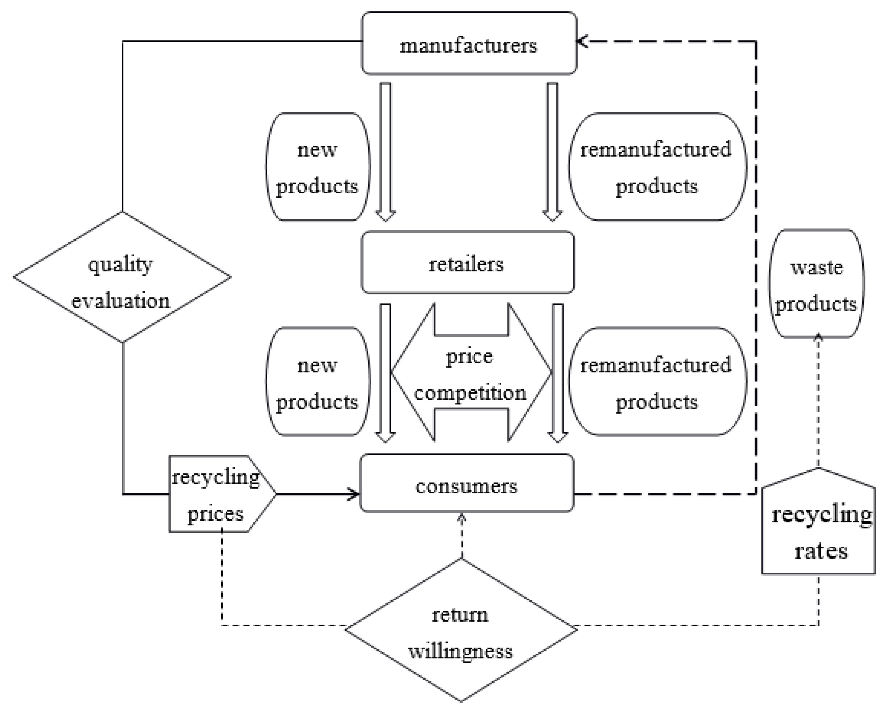
This study aims to construct a Stackelberg game model of closed-loop supply chains with the manufacturer as the leader, including single manufacturers, retailers, and consumers, as shown in Figure 1. The manufacturer can produce new products, and at the same time, it can remanufacture the returned products that have been collected from the end users. Consumers show a different willingness to pay for new and remanufactured products (consumer willingness to pay for remanufactured products is not higher than that for new products), and therefore, the demand for new and remanufactured products depends on the retail price. The manufacturer has to evaluate the quality of the returned products while collecting waste products from consumers, and gives consumers a recycling subsidy according to the quality of the recycled products, in addition, the recycling price has an impact on recycling rates. A high recycling price means that consumers are more willing to return the waste products and the returning possibility increases, which indicates that the recycling rate is higher. Initially, the manufacturer determines the wholesale price of new and remanufactured products. Subsequently, different recycling prices for end users are determined according to the quality of the returned products. Eventually, the retailer determines the demand and the retail price of new and remanufactured products, to maximize its profits.
3.2. Symbol Descriptions and Model Hypotheses
For the convenience of modeling, variables are introduced here, and the relevant definitions can be seen in Table 1.
The game participants in the model include manufacturers, retailers, and consumers, which is a dynamic game. Without changing the nature of the research questions, the assumptions in the model are as follows.
- (1)
- The product only can be recycled and remanufactured once, and similar products include photocopiers, computers, and mobile phones, as examples [23].
- (2)
- Although the quality of waste products varies from one piece to another, the quality of the remanufactured products is the same after being processed by remanufacturing technology. That is, the wholesale and retail prices of remanufactured products are undifferentiated, while there is a difference in the cost of the remanufacturing processes.
- (3)
- With sufficient productivity, the manufacturer is able to satisfy the market and the retailer’s demand.
- (4)
- Only the waste product, where the cost of the remanufacturing processes is less than that of manufacturing new products, can be recycled, so that remanufacturing is profitable. In addition, the production cost is less than the wholesale price, namely . In other words, for , the minimum quality coefficient is and .
- (5)
- The new products that were sold in the previous period and recycled in the present periods can be used for remanufacturing, and hence .
- (6)
- The manufacturer, the retailer, and the consumer aim to maximize their respective profits. In the supply chain, the manufacturer is the leader of game, while the retailer is the follower.
3.3. Demand Function
The waste products after remanufacturing can reach the quality level of new products, whereas there is a gap between consumer acceptance of the new and remanufactured products. In other words, there is a difference in the degree of willingness to pay for new and remanufactured products. According to the assumption of Ferrer and Swaminathan [11], when the market capacity is , it is assumed that the consumer willingness to pay for new products is subject to the even distribution from 0 to . The willingness to pay for remanufactured products is . In light of the consumer utility theory, consumers choose new or remanufactured products based on the degree of utility. The utility for consumers to opt for new or remanufactured products is and , respectively.
When the consumer’s utility of purchasing new products is greater than that of remanufactured products, namely and , it satisfies , and thus, below is the expression of the demand function of new products.
When the consumer’s utility of purchasing remanufactured products is greater than that of new products, namely and , it satisfies , and hence, below is the expression of the demand function of remanufactured products.
3.4. Cost Function in the Remanufacturing Process
In terms of the remanufacturing of returned products, the first step is dismantling and cleaning the waste products and then detecting the components. The detection results can be categorized into two types. One type is the repairable components, which can directly enter the remanufacturing stage, the other type is that which cannot be repaired because of the high degrees of damage, which need to be replaced by new components. Subsequently, the repaired components and the new replaced parts are re-assembled, thus leading to the remanufactured products, which eventually can be packaged [24]. The cost of the remanufacturing process consists of the material replacement cost and the human cost of material replacement , as well as the cost (the fixed constant) of the same links in the remanufacturing process, such as dismantling, detecting, cleaning, and packaging. The returned products possess different qualities, and thus the material replacement cost varies. The high quality of returned products means fewer unrepairable parts. The quality coefficient in this article is , showing the quality of the returned products. A higher quality coefficient means a higher quality of returned products. It is assumed that the probability density function of the quality coefficient of the returned products is , which can be achieved from sampling statistics.
When the quality coefficient of the waste products is , the cost of the remanufacturing process can be expressed as below.
Below is the average remanufacturing cost per unit of remanufactured product.
3.5. The Function of Recycling Prices
The total cost of remanufacturing covers the recycling cost (recycling price) and the cost of the remanufacturing processes. The wholesale price of the remanufactured products is the sum of the remanufacturing cost and the manufacturer’s profits [25], namely . The recycling price of the returned products with the recycling quality coefficient should be expressed as below.
It can be seen from the equation that a rise in the quality of product returns, namely, when the quality coefficient of product returns is greater, it means a higher recycling price for returns.
3.6. The Function of Recycling Rates
In terms of product returns with a certain quality coefficient, the recycling rate is the linear function of the recycling price. With a rise in the recycling price, the recycling rate goes up. The literature shows that the basic function between the recycling rate and the recycling price is expressed as follows ( [26].
In terms of the quality coefficient of the returned products, it is assumed that the minimum recycling price is , with the corresponding minimum recycling rate of ; it is assumed that the maximum recycling price is , with the corresponding recycling rate of , and the manufacturer sets the recycling price as . The minimum recycling price is , namely free recycling. In this case, consumers do not return waste products to the manufacturer without a price subsidy. According to Assumption 4, it is clear that the maximum recycling price is . In this case, the corresponding maximum recycling rate is a fixed constant, and , below, is the recycling rate with the quality coefficient of the returned products.
With the uncertain quality of product returns, below, is the average recycling rate.
3.7. The Function of Recycling Cost of Waste Products
The recycling cost is created when the manufacturer recycles the waste products, which is the cost of giving the end consumers who return waste products a price subsidy.
In terms of waste products with a quality coefficient , the recycling cost is multiplied by the recycling quantity and the recycling price. Below is the expression.
With the uncertain quality of product returns, below is the total recycling cost.
4. Modeling and Solutions
This model is a common two-stage game model of supply chains. The manufacturer is the Stackelberg leader, and the game sequence is as follows. The first step is that the manufacturers determine the wholesale price of the new and remanufactured products, expressed as and , respectively, by gaming with the retailer. Subsequently, the retailer determines the retail price of the new and remanufactured products, expressed as and , and and , respectively, by gaming with the consumers. In the game of a closed-loop supply chain, the optimal pricing decisions of production in the supply chain members are solved by backward induction.
4.1. Retail Prices of New and Remanufactured Products Determined by Retailers
Below is the retailer’s optimal profit function.
The first part of the target function shows the profits that are gained by the retailer selling new products, and its second part is the profits that are gained by the retailer who is selling remanufactured products. Because, the fact that remanufactured products are made by remanufacturing the returned products, the first constraint shows that the production of remanufactured products does not exceed the recycling quantity of the returned products in the preceding period, and the second constraint can ensure that the sales are not negative.
Proposition 1.
When,, below is the retailer’s optimal pricing.
Below is the optimal demand with this pricing.
The proof can be found in Appendix A.
4.2. The Wholesale Price Determined by the Manufacturer for New and Remanufactured Products
Below is the manufacturer’s optimal profit function.
The manufacturer can gain profits by selling new and remanufactured products to retailers. At the same time, the manufacturer needs to provide a recycling price for end users to collect the waste products for remanufacturing. The first part of the target function shows that profits that are gained by the manufacturer from selling new products, and the second part is the profits that are gained by selling remanufactured products. The third part is the recycling cost that is paid by the manufacturer for recycling the waste products.
Proposition 2.
The manufacturer’s optimal wholesale and recycling prices of new and remanufactured products are as follows.
Therein,
is correlated with , but it is independent of . The proof can be seen in Appendix B.
The backward induction is applied. Substituting the optimal wholesale price of the new and remanufactured products and the recycling rate, which is derived from Proposition 2, into the optimal retail price of the new and remanufactured products and the demand that is set by the retailer from Proposition 1, the manufacturer’ and retailer’s profits can be solved. It can be shown in Table 2.
5. Analyses of Examples
In light of the examples and data of a manufacturer of certain electronic products (Guo and Li et al. [27]), and the assumption of the quality coefficient subject to even distribution (Huang and Guo [28]), it is assumed that , , , , and the specific parameter setting can be seen in Table 3. To ensure there is no imaginary root for , now . Based on the results of Table 2, the impact of the profit rate of the unit remanufactured products that are sold by the manufacturer and the consumer preference coefficient for the remanufactured products on the remanufacturing decisions by the supply chain members is analyzed.
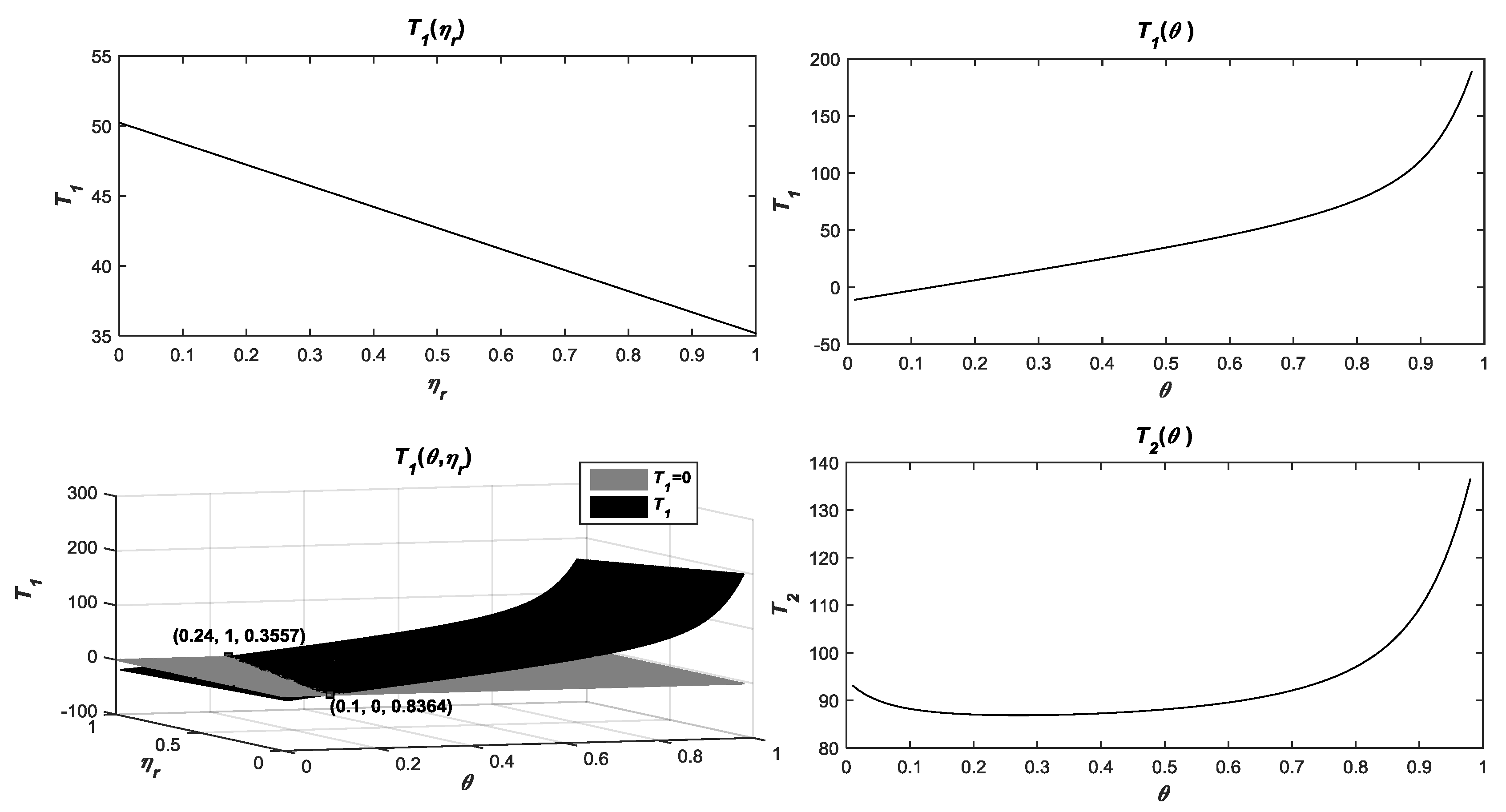
In order to ensure that the manufacturer can make both new and remanufactured products, must be satisfied, and the recycling rate is . Table 2 reflects the relationships among , and the parameters. is correlated with . In Figure 2, shows that when , varies with . shows that when , varies with . reflects how . can be influenced by . . is only correlated with and is not linked with . shows that varies with . It can be seen from the optimal decision from Table 2 that the recycling rate . is not correlated with , but it is only related with . Figure 3 shows the relationship between and .
It can be seen from Figure 2 that decreases with a rise in , but that it increases with a rise in . shows that when , satisfies . The reason for this is that remanufacturing is not profitable for the manufacturer if consumer acceptance of remanufactured products is so extremely low that the manufacturer only makes new products and abandons the market of the remanufactured products. When , can be an arbitrary number within . When , the value range is limited. This is because the price of the remanufactured products cannot be too high if the consumer acceptance of remanufactured products is rather low. Hence, the unit profit rate of remanufactured products cannot be too high. Also, , Figure 2 shows that when , is satisfied, and thus .
It can be seen from Figure 3 that the recycling rate increases with a rise in . When , is satisfied. In summary, to ensure that the manufacturer makes profits in remanufacturing, namely, when the profit that is gained by the manufacturer is greater than that when remanufacturing isn’t conducted, .
5.1. Impact of on the Decisions of Supply Chain Members
5.1.1. Impact of on the Manufacturer’s Decisions
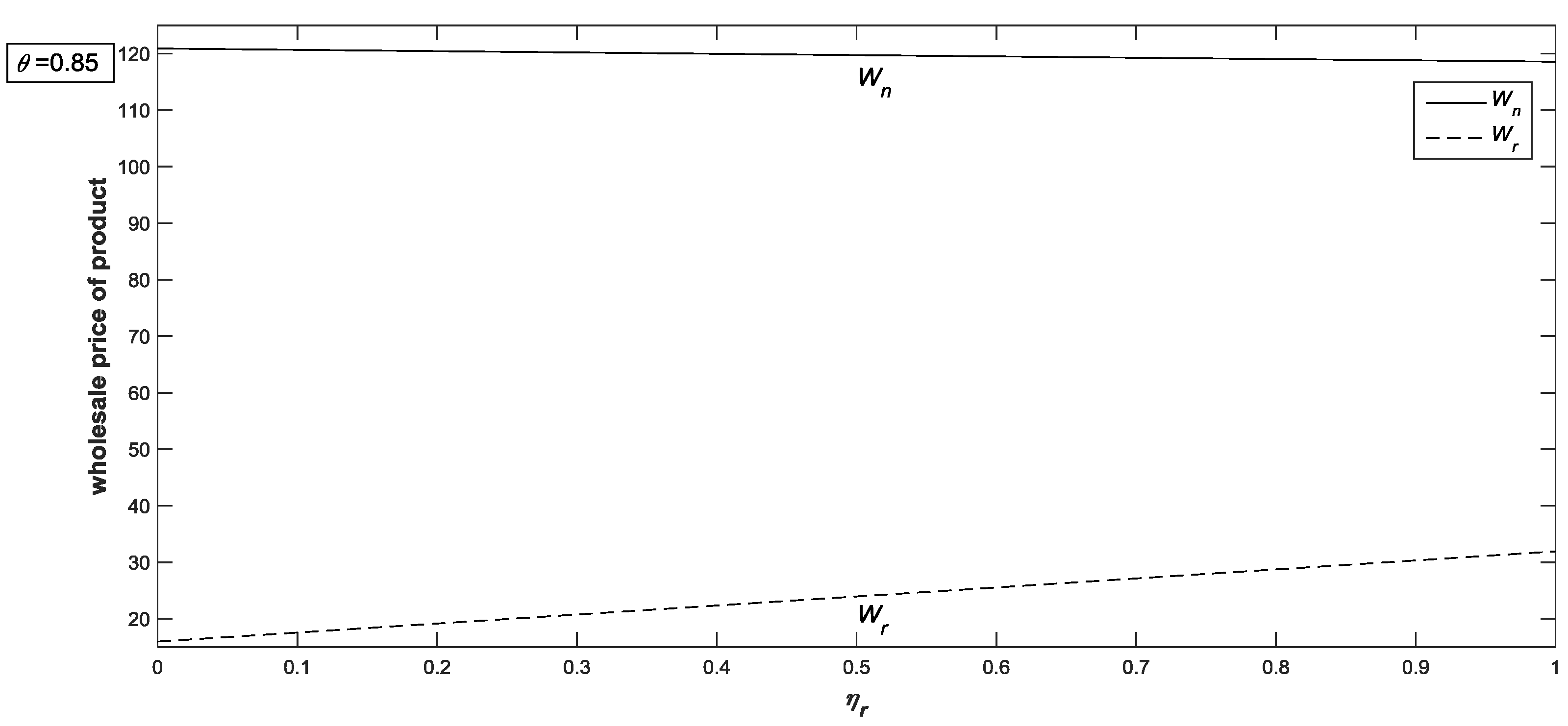
It can be seen from the optimal decision in Table 2 that the variations of only influence the wholesale price of new and remanufactured products that are set by the manufacturer (Figure 4). The optimal recycling price that is set by the manufacturer is correlated with the consumer preference for remanufactured products and the quality coefficient of the returned products, but it is not related with profit rate of the unit remanufactured product that is made by the manufacturer. That is because the variations of enable the wholesale price of the remanufactured products to change, while the unit remanufacturing cost (the sum of the unit remanufacturing process cost and the recycling price) remains unchanged. Therefore, the recycling price varies inversely with the cost of the unit remanufacturing process, but is not related with . Also, the recycling rate is not correlated with . When the impact of the manufacturer’s profit rates of the unit remanufactured product on the decisions of supply chain members is analyzed, .
It can be seen from Figure 4 that the optimal wholesale price of remanufactured products rises with an increase in the profit rate of the unit remanufactured product that is determined by the manufacturer, while the optimal wholesale price of new products tends to decline. The rising rate of the wholesale price of remanufactured products is greater than the decreasing rate of the wholesale price of new products. Hence, the gap between the wholesale price of the new and remanufactured products diminishes with a rise in . This suggests that if the manufacturer wants to earn more profits in remanufacturing, the wholesale price of new products drops when the wholesale price of remanufactured products increases. Also, the rise in the wholesale price of remanufactured products is greater than the fall in the wholesale price of new products.
5.1.2. Impact of on the Retailer’s Decisions
The optimal decision in Table 2 clearly shows that the optimal retail price that is established by the retailer and the demand are independent of .
It can be seen from Table 4 how influences the retailer’s optimal decision, depending on the relationship of and the equation . does not affect , because decreases with a rise in , and increases with a rise in . With a varying , the changing rate of is less than that of . When , the changing rate of is less than that of . In this article, it is assumed that the decreasing rate of with is the same as the increasing rate of with . Hence, does not affect . The optimal retail price that is set by the retailer and the demand are independent of .
5.2. Impact of on the Supply Chain Members’ Decisions
5.2.1. Impact of on the Manufacturer’s Decisions
(1) Impact of on the manufacturer’s wholesale prices
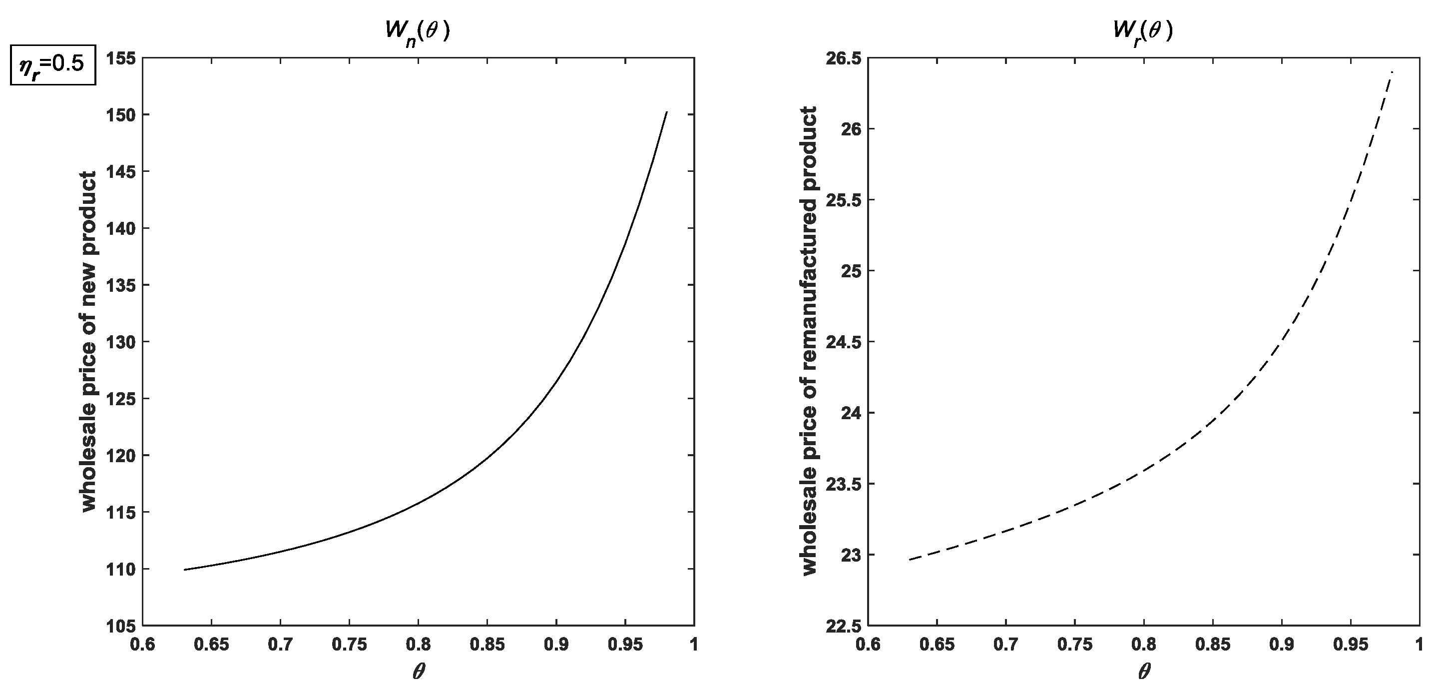
When the impact of the consumer preference coefficient of remanufactured products on the decision of supply chain members is analyzed, it is assumed that . Figure 5 indicates the impact of on the manufacturer’s decision on wholesale price.
It can be seen from Figure 5 that with a rise in consumer acceptance of remanufactured products, the optimal wholesale price that is established by the manufacturer for new and remanufactured products tends to increase. When remanufactured products are accepted, their prices go up. However, the cost of producing the unit remanufactured product is much lower than that of new products, and hence, when the wholesale price of the remanufactured products rises, the manufacturer tends to raise the wholesale price of the new products so that the profits of the new products will step up.
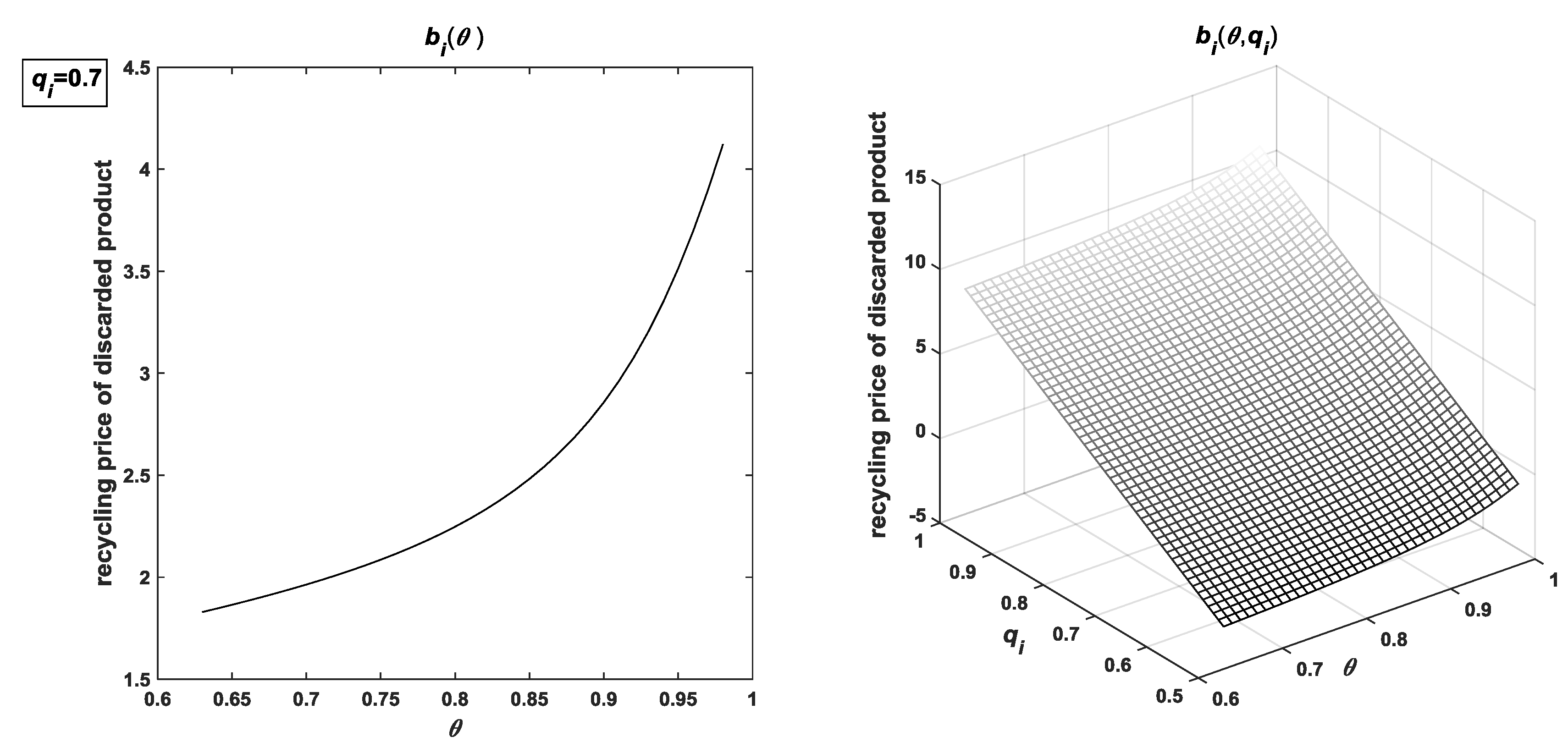
(2) Impact of on the manufacturer’s decision on recycling prices
In the Figure 6, shows how affects the recycling price, and . The figure shows that the recycling price increases with a rise in , and that the rate of rise constantly goes up. That is because the demand for remanufactured products increases when the consumer acceptance of remanufactured products grows, and thus, the manufacturer requires more returned products for remanufacturing. When the manufacturer increases the recycling price for returned products, the end users with waste products are more willing to return their old products, and thus, the manufacturer can collect more returned products for remanufacturing. In the Figure 6, illustrates how the optimal recycling price that is set by the manufacturer can be affected by consumer preference and the quality coefficient of the returned products simultaneously. This figure shows that the recycling price increases with the increase of the quality coefficient of the returned products. The reason is that the greater quality coefficient of the returned products means lower degrees of damage, re-manufacturability increases, and fewer replacement materials are required. As a result, more subsidies for returned products are provided for the end consumers.
5.2.2. Impact of on the Retailer’s Decision
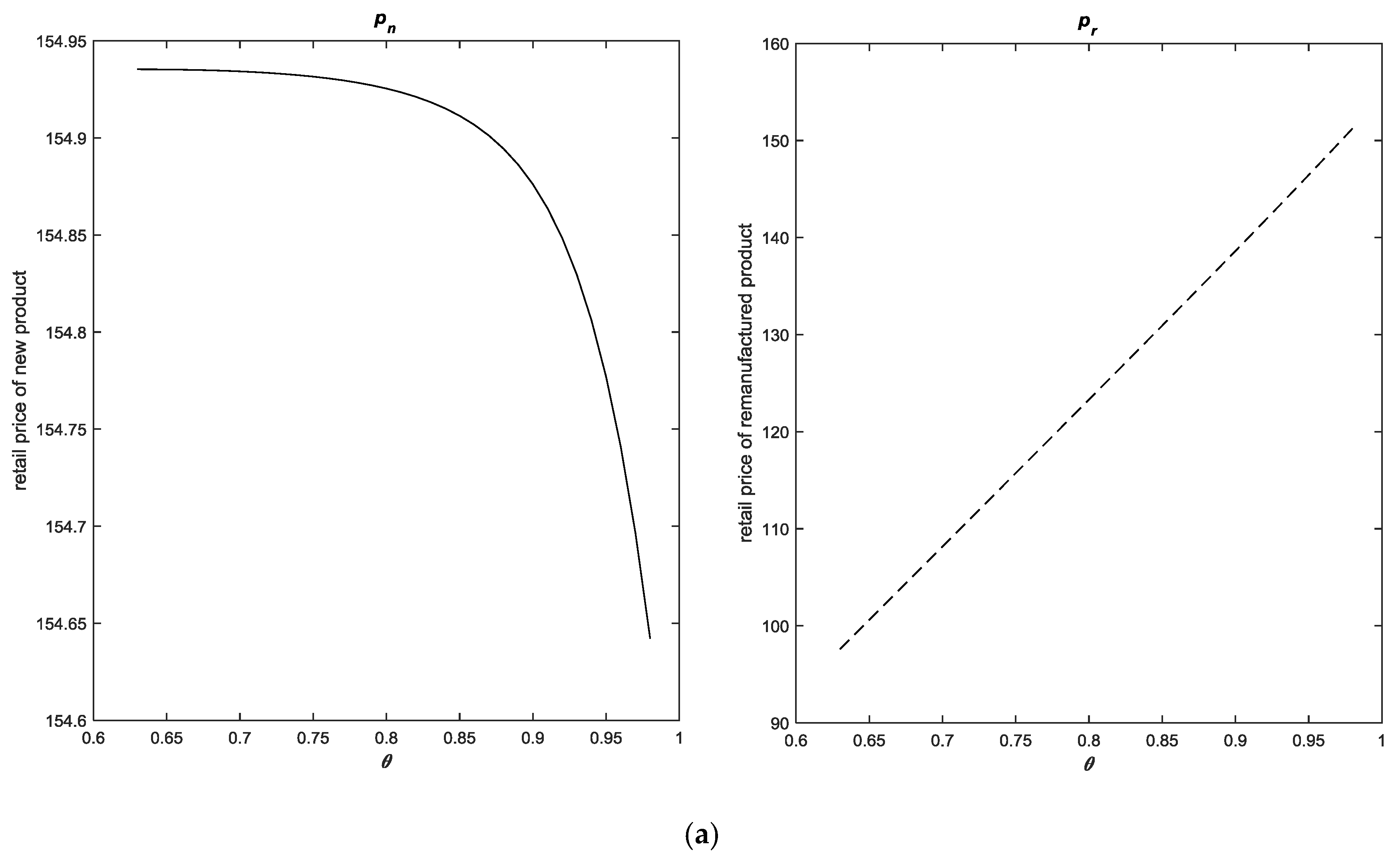
Impact of on the retailer’s decision can be seen in Figure 7, in which 7a shows how the retail price of new and remanufactured products is affected by and 7b shows that how has an effect on the demand for new and remanufactured products.
It can be seen from Figure 7a that the retail price of remanufactured products increases with a rise in , while the retail price of new products constantly drops. When is more than a certain value (around 0.85), the retail price of new products declines dramatically. The main reason is that consumers accept remanufactured products and they believe that the quality of remanufactured products approximates that of new products. Their wiliness to pay for remanufactured products is close to that of new products, and the retail price of remanufactured products is also close to that of new products. When is smaller, there is a significant difference between prices of new and remanufactured products. As a result, when increases to a certain value, the retail price of new products declines sharply. Figure 7b shows that the demand for new products constantly reduces with a rise in , while the demand for remanufactured products goes up constantly. When the consumer acceptance of remanufactured products increases, they are more willing to purchase remanufactured products. Therefore, the demand for new products drops. Additionally, the price of remanufactured products is lower than that of new products. Hence, the market share of remanufactured products increases gradually with a rise in .
5.2.3. Impact of on Profits
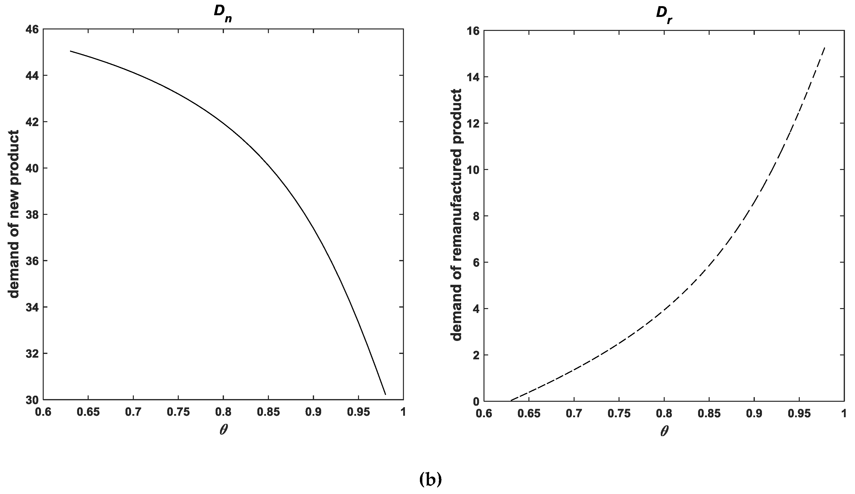
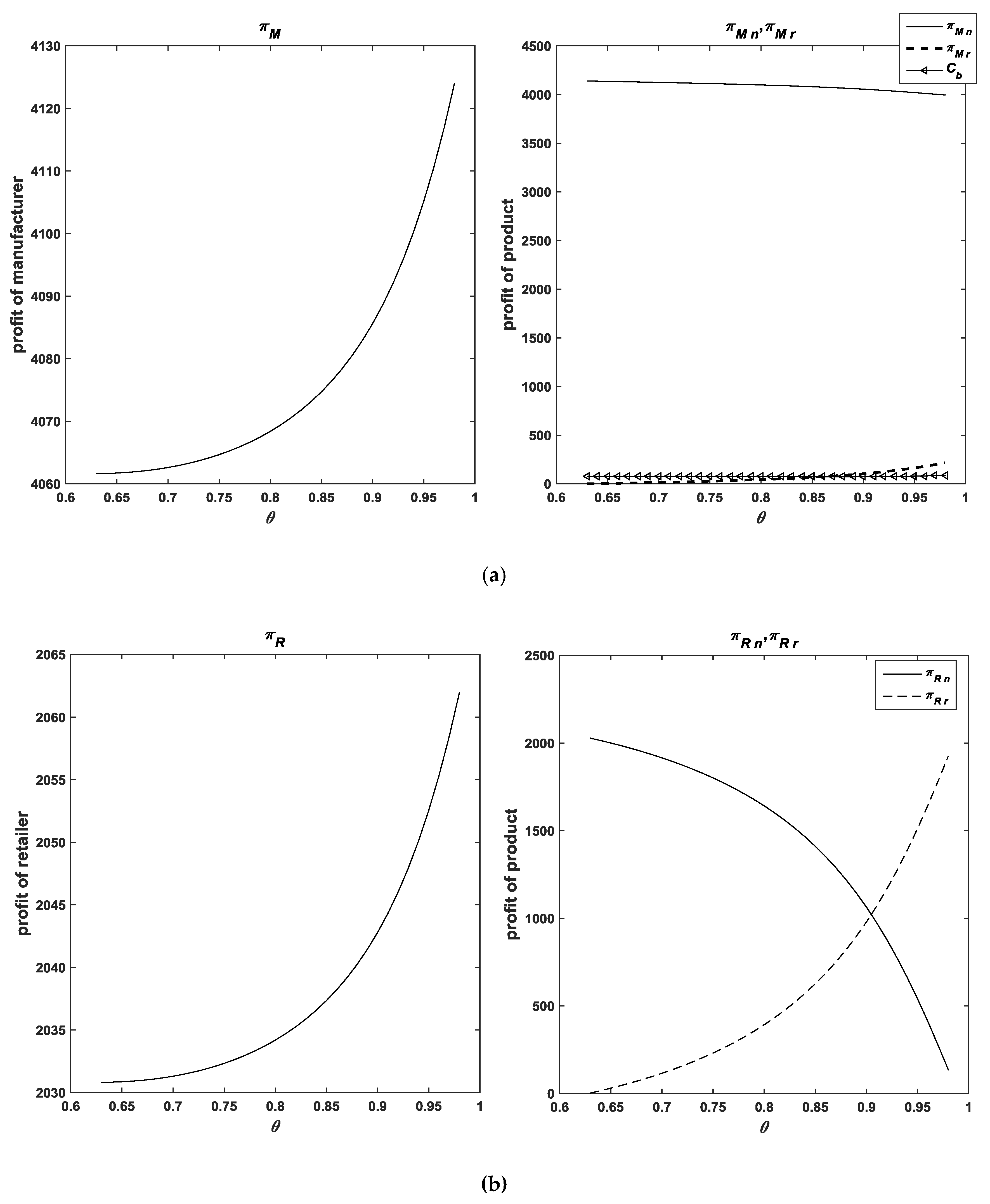
Figure 8 shows the impact of on the profits of the manufacturer and the retailer. Figure 8a shows how affects the manufacturer’s profits, and Figure 8b shows that how influences the retailer’s profits. The left figure shows that the total profits of the manufacturer or the retailer vary with . The right figure indicates the profits of new products and the profits of remanufactured products that are gained by the manufacturer, the recycling cost of the manufacturer , the profits of new products , and the profits of remanufactured products , that are gained by the retailer.
It can be seen from Table 2 that the profits of the manufacturer are always double those of the retailer when the manufacturer is the leader in the Stackelberg game. Figure 8 shows that the profits of the retailer and the manufacturer increase with a rise in . It can be seen from 8a that the manufacturer’s profits mainly come from the new products and that the profits of new products decline with a rise in . However, the profits of the remanufactured products and the total recycling costs increase with a rise in . Figure 8b shows that the retailer gains fewer profits from selling new products but more profits from selling remanufactured products. When is greater than a certain value (around 0.9), the retailer gains more profits from selling remanufactured products than from selling new products. When is greater, the consumer willingness to pay for remanufactured products approximates that for new products. In this case, the price of remanufactured products is lower than that of new products, leading to a greater demand for remanufactured products, and therefore, the retailer gains more profits from selling remanufactured products.
6. Conclusions
This article considers that consumers use their products differently, leading to the distinct qualities of returned products (i.e., collection of waste products). Thus, the manufacturer’s recycling price and remanufacturing processes are affected, which is true in practice. This article is based on the differences in the consumer’s willingness to pay, and the difference in the recycling quality of the waste products, the recycling price function, recycling rate function, recycling cost function, and remanufacturing cost function have been improved. The closed-loop supply chain game model has been built, including the single manufacturer, single retailer, and consumers. The optimal pricing decision of the supply chain members has been derived to maximize their profits and analyses of the theory and examples that are related to the model have been presented. Below are some highlights of the findings.
(i) If the consumer acceptance of remanufactured products is quite high ( exceeds a certain value), then it is necessary for the manufacturer to recycle and remanufacture the returned products. (ii) When remanufacturing is profitable, the profit rate of the unit remanufactured products, which are set by the manufacturer, only has an influence on the manufacturer’s pricing decision, while this does not affect the manufacturer’s profits and the retailer’s decision. As a result, it is unnecessary to consider the parameter of the profit rate of the unit remanufactured products that are set by the manufacturer in making decisions. (iii) The recycling price that is set by the manufacturer is correlated with the quality of waste products and the consumer preference for remanufactured products, and the recycling price is linearly and positively correlated with the quality of the returned products. In terms of waste products with an identical quality coefficient, the recycling price can be higher if the consumer preference for remanufactured products increases. (iv) When remanufacturing is profitable ( exceeds a certain value), the profits of the manufacturer are always double those of the retailer, and the profits grow with a rise in the consumer preference for remanufactured products. More importantly, the retailer even gains more profits from selling remanufactured products than from selling new products. The manufacturer can gain more profits from new products when rises, and the manufacturer’s profits from remanufactured products decline when falls. However, the profits from selling new products are generally greater than those from selling remanufactured products.
The model that was built in this study can be further expanded. For example, waste products can be recycled several times, and thus it can be expanded to two or more periods. Additionally, the competition among a multitude of manufacturers and suppliers can be taken into account, and the market can evolve in the context of competition.
Author Contributions
Supervision, S.C., S.W. and K.K.L.; Writing—original draft, J.X.; Writing—review & editing, T.S.
Funding
This research received no external funding.
Acknowledgments
This paper is financially supported by the National Natural Science Foundation of China (71771080, 71790593, 71521061, 71642006 and 71473155).
Conflicts of Interest
The authors declare no conflict of interest.
Appendix A
Proof of Proposition 1
Below is the Hessian matrix of the retailer’s profit function.
Because , , the Hessian matrix is negative, and the profit function is concave, with the extremum. The KKT can be introduced to solve the optimal value, with as the corresponding multiplier of the slack variable, constructing the Lagrange function.
Below is its Karush–Kuhn–Tucker condition.
When , below is the solution.
The optimal demand is derived as follows.
From , can be derived.
From , has to be satisfied. ☐
Appendix B
Proof of Proposition 2
From Proposition 1, we can see that the optimal production of the new and remanufactured products is , respectively, and that the recycling cost is , and the manufacturer’s optimal profit function can be denoted as follows, after substituting.
Therein, .
The target function is complicated and the recycling rate is the denominator, including the function of the decision variable . It is troublesome to solve the function of the decision variable. Therefore, it is assumed that , and both the recycling rate and the wholesale price of the remanufactured products can be denoted by .
The target function is denoted as follows.
- (1)
- First of all, it is assumed that the first-order partial derivative of decision variable of the target function is 0, the extremum of the decision variable is derived.
From , the following can be derived.
To simplify the equation, assuming the following,
The two first-order partial derivatives above are equal to zero, which can be rewritten as follows.
can be derived from (a) in Equation (A4), and therefore . Combining (a) and (b) in Equation (A4), below is the result.
Substituting into the expressions of , and , the unitary cubic equation of , can be derived, namely,
A real root and a pair of conjugate imaginary roots can be solved. The imaginary roots do not conform to the reality, and thus they are ignored. Below are the solutions of the equation.
Therein,
It can be seen from the expression of that is correlated only with but not with .
- (2)
- Below is the proof that is the maximum point of the target function.
In terms of the target function,
To solve the Hessian matrix of the target function at , below is the denotation of the form of .
satisfies Equations (a) and (b), therefore,
If the manufacturer’s profit function is , then below is the Hessian matrix of .
Because ,
Therefore, the Hessian matrix of is negative, and the target function is maximum on . ☐
References
- Guide, V.D.R., Jr.; Harrison, H.P.; Van Wassenhove, L.N. The Challenge of Closed-loop Supply Chains. Interfaces 2003, 33, 3–6. [Google Scholar] [CrossRef]
- Sun, X. Study on Development Path of Third-party Logistics in Low Carbon Supply Chain. Environ. Sci. Manag. 2018, 43, 1–4. [Google Scholar]
- Govindan, K.; Paam, P.; Abtahi, A.R. A Fuzzy Multi-Objective Optimization Model for Sustainable Reverse Logistics network design. Ecol. Indic. 2016, 67, 753–768. [Google Scholar] [CrossRef]
- Cheng, J.; Li, B.; Gong, B.; Cheng, M.; Xu, L. The Optimal Power Structure of Environmental Protection Responsibilities Transfer in Remanufacturing Supply Chain. J. Clean. Prod. 2016, 97, 1–12. [Google Scholar] [CrossRef]
- Guide, V.D.R., Jr.; Li, J. The Potential for Cannibalization of New Products Sales by Remanufactured Products. Decis. Sci. 2010, 41, 547–572. [Google Scholar] [CrossRef]
- Nie, J.; Zhong, L. A Research on the Remanufacturing Models with Green Customers. Ind. Eng. J. 2018, 21, 9–18. [Google Scholar]
- Abbey, J.D.; Blackburn, J.D. Optimal Pricing for New and Remanufactured Products. J. Oper. Manag. 2015, 36, 130–146. [Google Scholar] [CrossRef]
- Ferrer, G.; Swaminathan, J.M. Managing New and Remanufactured Products. Manag. Sci. 2006, 52, 15–26. [Google Scholar] [CrossRef] [Green Version]
- Debo, L.G.; Toktay, B.L.; van Wassenhove, L.N. Market Segmentation and Product Technology Selection for Remanufacturable Products. Manag. Sci. 2005, 51, 1193–1205. [Google Scholar] [CrossRef] [Green Version]
- Ferguson, M.; Toktay, B. The Effect of Competition on Recovery Strategies. Prod. Oper. Manag. 2006, 15, 351–368. [Google Scholar] [CrossRef]
- Ferrera, G.; Swaminathan, J.M. Managing New and Differentiated Remanufactured Products. Eur. J. Oper. Res. 2010, 203, 370–379. [Google Scholar] [CrossRef] [Green Version]
- Wu, Y.; Xiong, Z. Production Strategies of the Original Equipment Manufacturer and Independent Operator under the Condition of Competition. Syst. Eng. Theory Pract. 2014, 34, 291–303. (In Chinese) [Google Scholar]
- Zhang, J.; Huo, J.; Zhang, Y. Coordination Strategy Designing in Closed loop Supply Chain Based on Pricing Game. J. Ind. Eng. Eng. Manag. 2009, 23, 119–124. (In Chinese) [Google Scholar]
- Hazen, B.T.; Boone, C.A.; Wang, Y. Perceived Quality of Remanufactured Products: Construct and Measure Development. J. Clean. Prod. 2017, 142, 716–726. [Google Scholar] [CrossRef]
- Shulman, J.D.; Coughlan, A.T.; Savaskan, C.R. Optimal Reverse Channel Structure for Consumer Product Returns. Informs 2010, 29, 1071–1085. [Google Scholar] [CrossRef]
- Feng, Y.; Zhang, Y. A System Dynamics Model for Evolutionary Game of Recycling Quality Inspection between the Manufacturer and Retailer. Logist. Eng. Manag. 2018, 40, 119–124. [Google Scholar]
- Wei, J.; Zhao, J. Pricing Decisions with Retail Competition in a Fuzzy Closed-loop Supply Chain. Expert Syst. Appl. 2011, 38, 11209–11216. [Google Scholar] [CrossRef]
- Guide, V.D.R., Jr.; van Wassenhove, L.N. Closed-loop Supply Chains: Practice and Potential. Interfaces 2003, 33, 1–2. [Google Scholar] [CrossRef]
- Denizel, M.; Ferguson, M.; Souza, G.C. Multiperiod Remanufacturing Planning with Uncertain Quality of Inputs. IEEE Trans. Eng. Manag. 2010, 57, 394–404. [Google Scholar] [CrossRef]
- Robotis, A.; Boyaci, T.; Verter, V. Investing in Reusability of Products of Uncertain Remanufacturing Cost: The Role of Inspection Capabilities. Int. J. Prod. Econ. 2012, 140, 385–395. [Google Scholar] [CrossRef]
- Guo, J.; Ya, G. Optimal Strategies for Manufacturing/Remanufacturing System with the Consideration of Recycled Products. Comput. Ind. Eng. 2015, 89, 226–234. [Google Scholar] [CrossRef]
- Bhattacharya, R.; Kaur, A. Allocation of External Returns of Different Quality Grades to Multiple Stages of a Closed Loop Supply Chain. J. Manuf. Syst. 2015, 37, 692–702. [Google Scholar] [CrossRef]
- Savaskan, R.C.; Bhattacharya, S.; Van Wassenhove, L.N. Closed-Loop Supply Chain Models with Product Remanufacturing. Manag. Sci. 2004, 50, 239–252. [Google Scholar] [CrossRef]
- Bulmus, S.C.; Zhu, S.X.; Teunter, R. Competition for Cores in Remanufacturing Bulmus. Eur. J. Oper. Res. 2014, 233, 105–113. [Google Scholar] [CrossRef]
- Yuan, K.; Ma, S.; He, B. Study on Pricing Mechanism of Cores for Remanufacture Considering Returned Quality. Modul. Mach. Tool Autom. Manuf. Tech. 2015, 12, 152–155. (In Chinese) [Google Scholar]
- Klausner, M.; Hendrickson, C.T. Reverse-Logistics Strategy for Product Take-Back. Interfaces 2000, 30, 156–165. [Google Scholar] [CrossRef]
- Guo, J.; Li, B.; Ni, M. The Selection of Take-Back Model of Remanufacturing Closed-Loop Supply Chain Based on WTP Differentiation. Chin. J. Manag. 2015, 12, 142–147. (In Chinese) [Google Scholar]
- Huang, Z.; Guo, J.; Gu, B. Optimal Operation Strategy of the Closed-Loop System by Considering Recycling Product Quality and Price Level. Ind. Eng. Manag. 2014, 19, 36–41. (In Chinese) [Google Scholar]
Figure 1.
Closed-loop supply chains with manufacturers’ remanufacturing.

Figure 2.
varying with the parameters of .

Figure 3.
varying with the parameter of .

Figure 4.
Impact of varying on the wholesale price of new and remanufactured products.

Figure 5.
Impact of varying on the wholesale price of new and remanufactured products.

Figure 6.
Recycling prices.

Figure 7.
(a) Impact of varying on the retail price of new and remanufactured products (b) Impact of varying on the demand for new and remanufactured products.
Figure 7.
(a) Impact of varying on the retail price of new and remanufactured products (b) Impact of varying on the demand for new and remanufactured products.


Figure 8.
(a) Impact of on the manufacturer’s profits, (b) Impact of on the retailer’s profits.


Table 1.
Variables and definitions.
| Variables | Definitions |
|---|---|
| Unit production cost of new products | |
| Unit material replacement cost refers to the cost of new components when parts cannot be repaired in the remanufacturing process | |
| Human cost caused by alternative materials in the process of remanufacturing of products, , | |
| The cost caused by the same links in the remanufacturing process such as disassembly, detection, cleaning, and packaging, which is a fixed constant | |
| The quality coefficient of product returns, , ; a rise in means that the quality of returns is higher. | |
| The minimum quality coefficient of product returns | |
| The unit cost of remanufacturing process when the quality coefficient of product returns is , | |
| The price subsidy which manufacture offers the end users who return waste products when the quality coefficient of product returns is | |
| The unit cost mean value of remanufacturing process with uncertain quality of product returns | |
| The profit rate gained by manufacture when one unit of remanufactured product is sold to the retailer | |
| The recycling rate when the price of product returns is with the quality coefficient | |
| The mean value of recycling rate with uncertain quality of product returns | |
| The unit wholesale price of new products | |
| The unit wholesale price of remanufactured products | |
| The unit retail price of new products | |
| The unit retail price of remanufactured products | |
| The market demand of new products | |
| The market demand of remanufactured products | |
| The coefficient of consumer preference for remanufactured products, , |
Table 2.
The manufacturer’s and retailer’s optimal decisions.
| Decision Variables | Optimal Decisions |
| . | |
Table 3.
Model parameters.
| Parameters | Values | Units | Symbols | Calculated Values |
|---|---|---|---|---|
| A | 200 | Sets | 0.4531 | |
| 18 | Yuan/set | 12.4 | ||
| 0.2 | / | 0.2226 | ||
| 7 | Yuan/set | 1.8489 | ||
| 0.6 | / | 17.0982 |
Table 4.
Reduced forms of the retailer’s optimal decisions.
| Decision Variables | Optimal Decisions | Forms |
|---|---|---|
are not correlated with ) | ||
© 2018 by the authors. Licensee MDPI, Basel, Switzerland. This article is an open access article distributed under the terms and conditions of the Creative Commons Attribution (CC BY) license (http://creativecommons.org/licenses/by/4.0/).
Share and Cite
MDPI and ACS Style
Shu, T.; Xu, J.; Chen, S.; Wang, S.; Lai, K.K. Remanufacturing Decisions with WTP Discrepancy and Uncertain Quality of Product Returns. Sustainability 2018, 10, 2123. https://doi.org/10.3390/su10072123
AMA Style
Shu T, Xu J, Chen S, Wang S, Lai KK. Remanufacturing Decisions with WTP Discrepancy and Uncertain Quality of Product Returns. Sustainability. 2018; 10(7):2123. https://doi.org/10.3390/su10072123
Chicago/Turabian StyleShu, Tong, Jiajia Xu, Shou Chen, Shouyang Wang, and Kin Keung Lai. 2018. "Remanufacturing Decisions with WTP Discrepancy and Uncertain Quality of Product Returns" Sustainability 10, no. 7: 2123. https://doi.org/10.3390/su10072123
Note that from the first issue of 2016, this journal uses article numbers instead of page numbers. See further details here.