An Original Approach Combining CFD, Linearized Models, and Deformation of Trees for Urban Wind Power Assessment


1
Department of Climatology and Environmental Meteorology, Institute of Geoecology, Technical University of Braunschweig, 38106 Braunschweig, Germany
2
Institute of Geography and Spatial Planning, Center of Geographical Studies (ZEPHYRUS/Climate Change and Environmental Systems Research Group), Universidade de Lisboa. Ed. IGOT, R. Branca Edmée Marques, 1600-276 Lisbon, Portugal
3
Faculty of Environmental Sciences and Natural Resources, Albert-Ludwigs-University Freiburg, 79085 Freiburg, Germany
4
Research Center Human Biometeorology, German Meteorological Service, 79104 Freiburg, Germany
*
Author to whom correspondence should be addressed.
Sustainability 2018, 10(6), 1915; https://doi.org/10.3390/su10061915
Submission received: 11 April 2018
/
Revised: 30 May 2018
/
Accepted: 4 June 2018
/
Published: 7 June 2018
(This article belongs to the Special Issue Sustainable Energy Development under Climate Change)
Abstract
:Wind energy is relevant to self-sufficiency in urban areas, but the accuracy of wind assessment is a barrier to allowing wind energy development. The aim of this work is to test the performance of the Griggs-Putnam Index of Deformity of trees (G-PID) over urban areas as an alternative method for assessing wind conditions. G-PID has been widely used in open terrains, but this work is the first attempt to apply it in urban areas. The results were compared with CFD simulations (ENVI-met), and finally, with the linear model WAsP to inspect if deformed trees can offer acceptable wind power assessments. WAsP (meso-) and ENVI-met (micrometeorological model) showed similar results in a test area inside the University of Lisbon Campus. All trees showed a deformation with the wind direction (S and SE). The mean G-PID wind speed for all trees was 5.9 m/s. Comparing this to the ENVI-met simulations results (mean speed for all trees was 4.25 m/s) made it necessary to adapt the index to urban terrains by reducing each Index Deformation class by about ~2 m/s. Nevertheless, more investigation is needed, since this study is just a first approach to this integrated methodology. Also, tree species and characteristics were not taken into account. These questions should be addressed in future studies, because the deformation of trees depends also on the tree species and phytosanitary conditions.
1. Introduction
In times of uncertainty related to climate change, the reduction of anthropogenic emissions of greenhouse gases to mitigate global warming and the use of renewable energies, such as solar and wind power energy, are alternative solutions to the consumption fossil fuels and nuclear power [1,2]. To achieve this “energy revolution”, it is important to know the potentials (energy payback, GHG decrease, etc.) and the limitations (energy supply system, storage, etc.) of new energy systems [2].
Urban areas are typically great energy consumers and major wasters, leading to an unbalanced metabolic model that poses an interesting environmental problem [3]. Besides that, cities will never be autonomous if they only depend on energy produced outside their borders (provided by others), and never be sustainable if they are supplied in large part by fossil fuels and nuclear power. The principle of attaining 100% renewable energy in cities has therefore been a goal pursuit since the late 90s [3]. Wind power could be one of the best options for producing sustainable energy systems, especially near windy coastal areas like the city of Lisbon [4].
However, the complicated urban fabric can lead to turbulent fluxes that can be harmful to small wind power systems, and force wind turbines to shut down or operate incorrectly. Looking at the wind flow characteristics in mesoscale urban areas, statistics show in a study concerning the wind speed modification in summer due to urban growth in Lisbon that the wind speed at 10 m height in the city is up to 30% lower than in open terrain [5]. The consequence of the wind speed decrease can affect ventilation conditions and lead to the impoverishment of air quality, health, and human comfort conditions. Furthermore, it can also affect the wind power potential for urban areas. Exceptions are microclimatic lee-twirls of high buildings and the jet effect in street canyons, which cause high wind speeds and strong gusts. Due to the complicated wind conditions in urban areas, they have to be reproduced by wind tunnel experiments or wind flow models (CFD) [6]. Wind profiles can also be important to show the influence of surface roughness on air flow.
Possible solutions to these problems are turbines on rooftops (known as “architecturally integrated”), installed in high, densely-built areas. These types of turbines are not very common, but interest in them is increasing. Other options for wind turbine installation are parks and generally partially open areas in cities where the influence of obstacles on the wind is minimized. The right height can prevent the influence of obstacles and turbulence [7]. Therefore, finding the best potential places for the installation of Small Wind Turbine (SWT) systems in urban areas is crucial for their implementation.
SWT are required for the production of electricity from wind for a home, farm, school or small business. A lot of advantages are associated with these turbines; for example, they cause reduced pressure on the local electricity grid, increased security that can provide back-up power to strategic applications like police stations or hospitals, increased local energy independence, increased property values, and much more [7].
In Portugal, a law from November 2014 encourages individuals to produce electricity from small systems (Decreto-Lei n.° 153/2014). Local production has the advantage of reducing loads and losses on network grids, and permits the direct use of electricity. The development of the legislation encouraging the efficient use of energy seeks to create a new paradigm to reduce greenhouse gas emissions, and to contribute to the energy balance of buildings, collectively contributing to the EU directive zero energy budget (Directive 2010/31/EU). However, due to the recent nature of this law, much work has yet to be done to encourage the citizens to produce their own energy; first of all, research about the best locations to install SWT (as well as the public acceptance [8]) is urgent.
As mentioned, Portuguese law allows the self-production of electricity, as well as the sale of generated power to the electric network. The fixation of the prices, fees, and paybacks will be the driving force vis a vis the level of future acceptance among the public. In Portugal, for all renewable energies, a micro production is typically under 11.04 kW (maximum for a condominium), while a mini production has a maximum power of 250 kW (Portuguese Ministry of Economy, [www.renovaveisnahora.pt/web/srm/entrada, last access in March 2015]; [9]).
The accurate micro-siting for SWT can be attained by using software and models like WAsP (Wind Atlas Analysis and Application Program), developed by the Wind Energy Department at Risø National Laboratory (DTU Wind Energy) coupled or independently used with CFD (Computational Fluid Dynamics) models [10].
Recent research [11] proposed a U-DTM methodology (a CFD couple with an urban digital terrain model) to assess wind power viability in a location to the west of the city of Lisbon. In line with these kinds of techniques, the methodology we propose in this research combines biomonitoring (G-PID: wind data through observation of wind-driven tree deformation [12,13]), linear (WAsP), and CFD (ENVI-met) modeling for the assessment of wind power potential in urban environments, where wind data is difficult to obtain.
Several studies used tree deformations to determine the prevailing wind direction, like that of Holroyd in 1970, who observed the flagging direction of 2000 trees in New York’s Whiteface Mountains [14]. Other studies about trees as indicators of wind speed are documented: the botanist R. F. Griggs was the first who found a correlation between the crown deformation of coniferous trees and wind intensity [15]. Weischet (1953), Thomas (1958), Barsch (1963) and Yoshino (1973) created other classifications [14].
2. Data and Methods
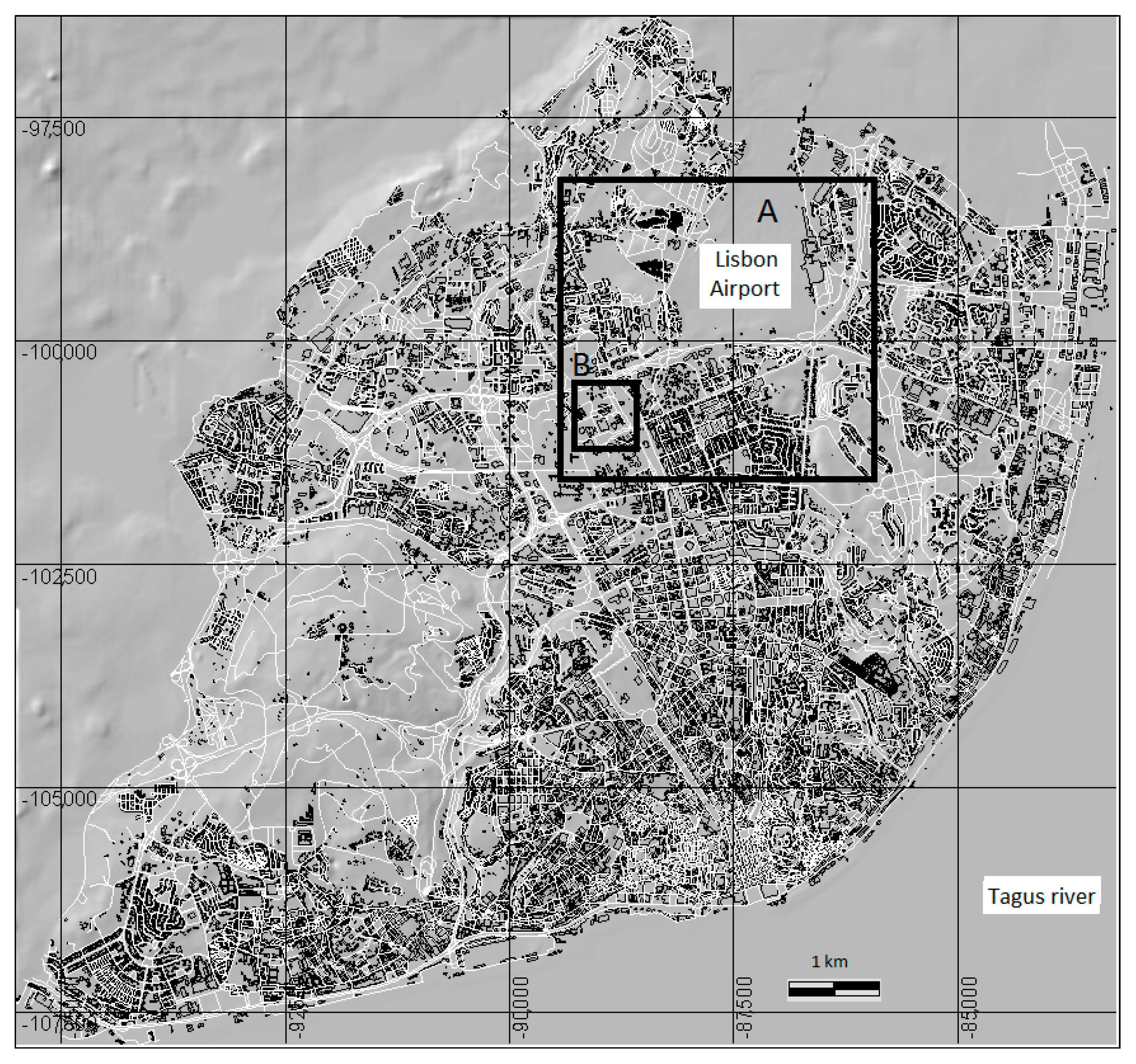
The experimental work presented in this paper is divided into two scales: (i) local (per definition e.g., Urban Heat Island (UHI) patterns spanning some kilometers) and (ii) micrometeorological (per definition e.g., an urban canyon). The first area (Figure 1A: 3.5 km × 3.5 km) is located in northern Lisbon, close to the Lisbon Airport. This area was chosen because it is a large open area that is well ventilated, and therefore, suitable for local simulations. For the local analysis, the necessary information about the study area and methodology will be introduced, and the general wind conditions analysis will be presented. This will be accomplished through meteorological data modeling with the WAsP 10 software (see description in Section 2.4).
The second scale/area (Figure 1B: 0.5 km × 0.5 km) is a neighborhood around the University of Lisbon (ULisboa, Lisboa, Portugal), where field work to assess street trees and their deformations by the wind was made. For the microscale assessment, two methodologies were used: the first was the application of the Griggs-Putnam Index of Deformity (G-PID) of the trees, which allowed us to create a map with predominant wind speed and directions around the buildings. The second methodology consisted of the micrometeorological modeling of the wind in the same neighborhood with ENVI-met [22]. This software uses CFD (Computational Fluid Dynamics) that will be described in the methodological Section 2.4. The results will serve as comparison and validation of the G-PID. This procedure will demonstrate the potential of this low cost methodology for assessing wind power potential through tree deformation in cities.
This paper is a first methodological assessment to assess the extent to which peripheral/low to medium density urban areas are suited to the installation of SWT. For the definition of low density urban areas, we considered peripheral open spaces with a ratio H/W (Height of the buildings/Width of the streets) below 0.6 and an urban roughness length (z0) (excluding green parks) inferior to 0.2 m [23], in the northern part of the city of Lisbon. For medium density areas, an H/W < 0.9 and a z0 < 0.6 m were considered. In the working area, there is about 58.5% flat (mostly the Lisbon Airport runways), low, and medium urban density, 31% high urban density, and 10.5% green spaces (Figure 2).
2.1. Site Description of Lisbon
Lisbon is located at 38°43′ latitude N and 9°9′ longitude W in the subtropical climatic zone. The city lies 30 km to the east of the Atlantic Ocean, and on the north bank of the Tagus River.
The city of Lisbon has 547,733 inhabitants in the municipal area and more than 2 million in the metropolitan area [24]. Its area extends to circa 84 km2 [4]. In the old city center, which lies on the Tagus River banks, the streets have a low aspect-ratio (H/W) due to their Roman and Muslim architecture heritage. In the newer (northern and northeast) part of the city, the H/W is clearly higher, and traffic is more intense. In general, the larger streets have a great effect on the urban climate (more absorption of direct radiation, because of less shadowing; more heating, because of the high traffic); however, the city’s prevailing winds from the north and northwest, and the sea breezes coming from the ocean, as well as the Tagus breezes, cause an effective ventilation of the urban climate of Lisbon [25,26,27]. The expansion of the city to the north, and the construction of higher buildings in the near future, will serve as obstacles for the wind flow, and constrain this effect [5], so that the UHI pattern (more intensely developed in the city center, because of insufficient ventilation due to the city structure around it) can expand to other areas [25].
Three main hills that can modify the city’s prevailing winds are located between Lisbon and the Atlantic Ocean: Sintra (500 m high), that lies to the west, Carregueira (250 m high), to the northwest, and Monsanto, close to the city (250 m high) to the west [4].
Lisbon has a Mediterranean climate, with generally warm temperatures, mild and rainy winters, and hot, dry summers (Koeppen classification “Csa”) [28]. The mean maximum air temperature occurs in August (1981–2010 Lisbon/Geofísico normal is 28.3 °C), one of the warmest months, with an absolute maximum of 41.8 °C. The mean minimum air temperature generally occurs in January (the coldest month of the year), and reaches 8.3 °C, while the absolute minimum occurred in March (0.2 °C). The annual mean air temperature is about 17 °C.
During winter, wind blows mostly from the southwest and the northwest, but during summertime (from June to August) the prevailing winds come more from the north and northwest. In summer, air temperatures and ventilation show a complex relationship, with the UHI being very dependent of wind speed and direction [25]. Also, the maritime air causes lower land air temperatures and increased humidity [4]. Because of air temperature and pressure differences between the Iberian Peninsula and the ocean, very strong northern wind systems can develop. These are caused by a high barometric gradient between the Azores high and the low-pressure area over the Iberian Peninsula [4], forming the well-known summer-“Nortada” [5].
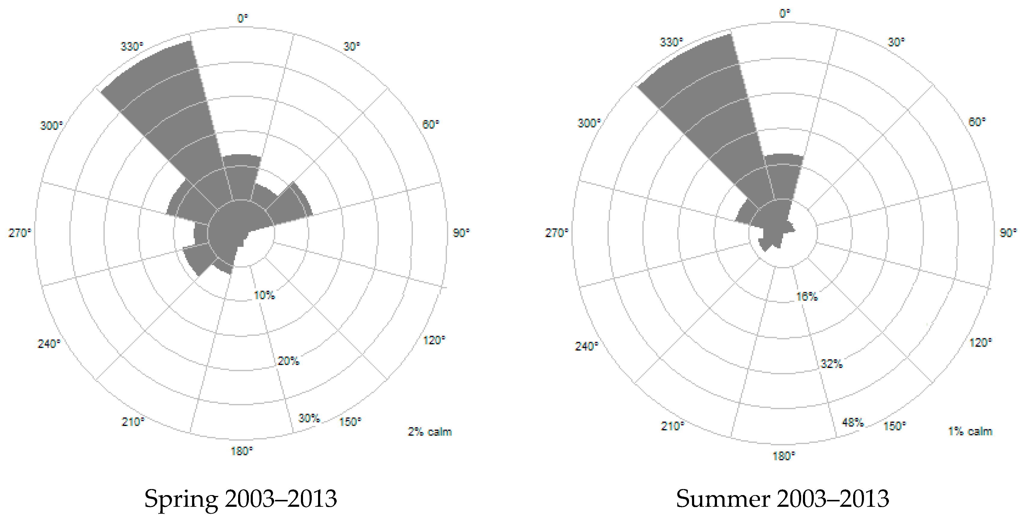
In Figure 3, spring and summer wind roses of the Lisbon Airport are shown (see Section 2.4.1 for metadata). This period represents the growing season for most of the trees in the city, and, as mentioned by Meneses and Lopes [21], it also corresponds to higher wind velocities that can shape tree canopies and trunks; this period is therefore most relevant to this study (to see wind regimes in all months/seasons see Section 3.1. Figure 6). The shapes and deformations can be correlated with an index of the average wind speeds in the streets (this process will be described in Section 2.3).
Because the city of Lisbon has a very constant wind regime in spring and summer with good power potential [21], it was chosen as the test area for this research.
2.2. Bioindicators
The observation of tree deformities is a good bioindicator of information about the average wind conditions in a region [21]. The wind can develop forces strong enough to turn out and bend trees, permanently changing the forms of trunks and canopies. This pressure is composed of the stationary resistance of the tree, and of the mass inertia in consequence of the gustiness of the wind. For the determination of the resistance coefficient (CD), big and healthy trees have to be considered. Also, trees smaller than 3 or 4 m and located too close to other structures (building, walls, etc.) should be avoided, because micro turbulent fluxes can yield erroneous data. It is unknown how many trees in the same area should be used to determine CD [29].
CD decreases with increasing wind speeds, and shows different values for different species and even within members of the same species. This means that there will be a general difference of CD between every single tree. Reasons for this are deficits in methodological approaches, and the different characteristics of every tree, which affect the aerodynamic roughness of the tree surface. Characteristics can be tree height, diameter, crown length, etc. Also, the health of a tree, the surface structure, duration of weather events, wind speeds and gustiness, as well as the type of soil and its humidity, are all important factors [29].
Besides this, the root formation as a function of the soil characteristics is important for tree stability. The influences of the wind on the roots increases with age, contact surface, and the degree of clearance of the vegetation; additionally, the reactions of trees depend on the soil type its physical condition. For example, loamy soil loses its stability in strong humidity [30]. Also, urban, artificial “soils” are frequently very different from natural ones, meaning that typically, trees have reduced life-spans and adaptability compared to those in the natural landscape [31].
Other effects of wind on trees are dependent on the strength and persistence of the wind e.g., light winds (<0.9 m/s) generally increase carbon dioxide uptake, causing accelerated photosynthesis and growth stimulation. Other studies have shown that stronger winds (>2.2 m/s) slow down plant growth [14]. The negative influences of stronger winds can be separated into the following categories: mechanical damage (breaking of branches or damaging leaves, abrasion, and defoliation), physiological responses (biochemical changes, e.g., the production of hormones), anatomical adaptations (changes in cell structure or tree shape), and morphological changes (deformation of tree crowns) [14].
2.3. Measurement of Tree Deformation for the Wind Speed Assessment
Strong winds can affect vegetation—an effect known as flagging—, especially in coniferous trees, that can become permanently deformed. The G-PID helps to determine the potential of a wind site by observing the shape of trees in the area of interest. This methodology is most useful in areas with few meteorological stations, as well as for estimating the average annual wind speed. Typically-observed sites are coastal regions, river valleys, and gorges, because of the strong channeling effect of the wind, and mountainous terrain, where wind data is rare, and its assessment may be very difficult. In the case of a wind speed assessment, trees have two advantages: their height, and the long periods over which they gather data. In fact, the G-PID can be used to estimate the mean wind speed relating the form of the trunk and the shape of the tree canopy with specific velocities [32]. The different G-PID deformation classes can be empirically taken from Hiester and Pennell [33], as shown in Table 1.
A complete survey, with all the variables needed to compute the index around the campus of the University of Lisbon (B in Figure 1), is presented later in Section 3.2 in Table 3. The right choice of trees is of great importance, and some were excluded in this research: one (number 8 in the inventory) presents a deformity caused by the proximity of the buildings, representing more turbulence than the mean wind speed, and was therefore rejected. Other causes of tree rejections to minimize data errors were: low crown densities (like number 15 and 20), deformations to W, and direction inconsistencies with known wind conditions. Some trees were affected by disease, or were artificially stabilized; others, where a lot of branches have been cut, have a modified weight balance making them unstable, and therefore, not useful for this research. Trees 8, 15, and 20 are listed in the inventory because it was necessary to check their G-PID to be sure that they could be rejected. Some other trees that are not present in the inventory had to be rejected immediately because of the various reasons listed above, i.e., no G-PID measurements were necessary.
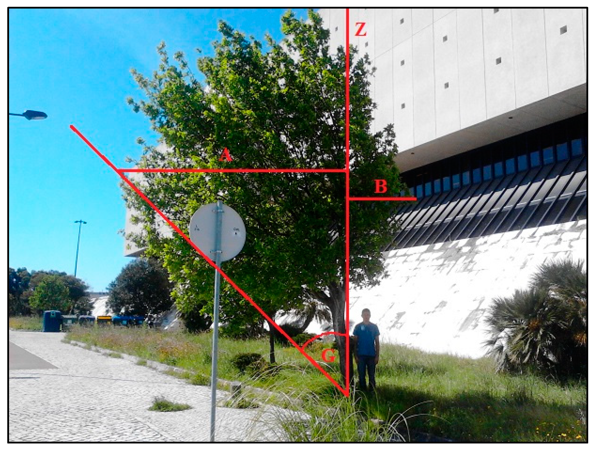
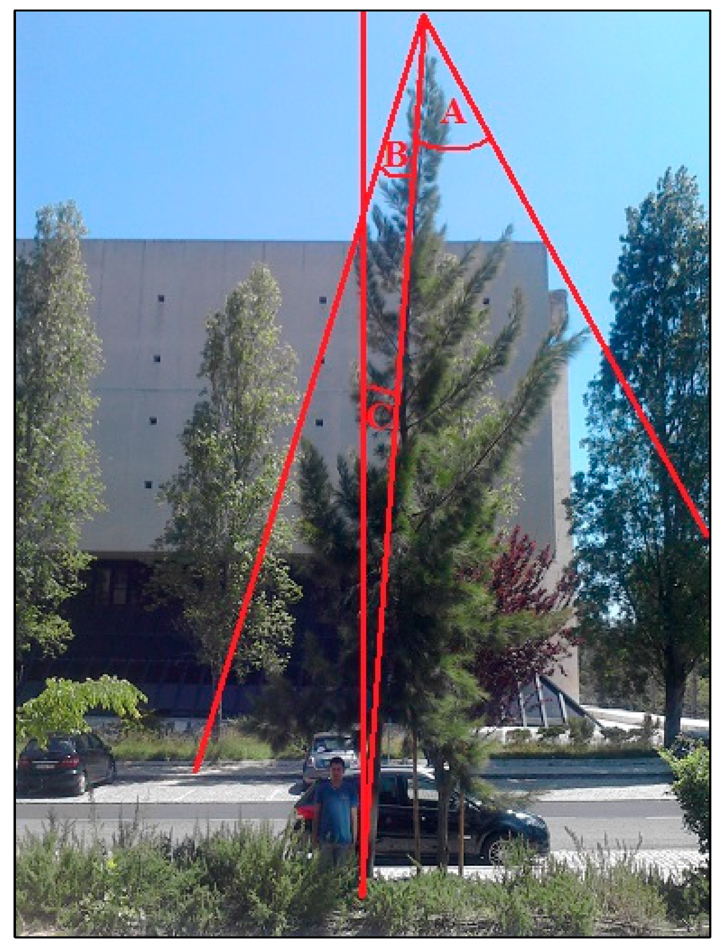
The G-PID method is easy to implement and can complement other wind power assessments that use models like WAsP and CFD. The measurements that are required to perform the G-PID are shown in Figure 4. These are manually computed from pictures taken of the recommended trees, i.e., those not close to walls, preferably on sidewalks, and isolated from other obstacles. The person in the pictures serves as a scale reference (~1.71 m high) to convert the measured values from cm to m (tree height Z, variables A and B for globose trees). The index was calculated using the measured variables that are described below in Equations (1) and (2).
Two algorithms can be used depending on the crown form of the tree. The indices are calculated as follows [20]:
For conical forms:
where Arad is the angle between axis Z and the farthest point of the crown to the lee side (in radian); Brad is the angle between axis Z and the farthest point of the crown to the windward side (in radian); and Grad is the angle between axes Z and Y (in radian). The value 0.785 is parameterized.
G-PID = (Arad/Brad) + (Grad/0.785)
For globose forms:
where A is the distance between axis Z and the farthest point of the crown to the lee side (in m), and B the distance between axis Z and the farthest point of the crown to the windward side (in m).
G-PID = (A/B) + (Grad/0.785)
2.4. Wind Data and Modeling
2.4.1. Wind Data
A ten-year, hourly dataset in 10 m AGL (wind speed, wind direction; from March 2003 to March 2013) from the Gago Coutinho meteorological station (station number WMO index: 08579; located near the Lisbon Airport, 38°46′00.0″ N 9°08′00.0″ W, at an altitude of 104 m and close to the study area) was used. The data was obtained from the National Climatic Data Center (NCDC, Asheville, NC, USA), specifically, from the National Oceanic and Atmospheric Association (NOAA) portal [http://www.ncdc.noaa.gov/land-based-station-data/find-station, 2013].
2.4.2. Models (ENVI-Met and WAsP)
CFD models, which can be used for wind engineering and wind power assessments, have been evolving for more than 50 years. The main difficulties during that time have been, e.g., the needed high grid resolutions, the complexity of the 3D flow-field, numerical problems in association with flows at sharp corners and the inflow and outflow boundary conditions, etc. These difficulties still pose limitations on CFD models; however, these difficulties continue to be addressed, and have, in recent years, been minimized. Other problematic questions concerning e.g., convective heat transfer, wind and acoustics, and wind energy in the built environment, will also have to be addressed in the future [34,35].
CFD offers the advantage of providing a detailed description of the flow in the observed area; it is a great complement to wind-tunnel measurements. Both tools are important, since many computational wind-engineering problems are too complex to be handled only by CFD models. As a conclusion, it is recommended that CFD be used together with wind-tunnel measurements for validation, if possible (e.g., when simulating buoyant flows) [34].
Examples of popular, state-of-the-art CFD software are OpenFOAM, ANSYS Fluent, and ENVI-met, about which a lot of literature can be found worldwide. All three differ in numerical methods, spatial and temporal specifications, turbulence models, and boundary conditions (e.g., inlet and outlet) [22,36]. OpenFOAM is a free, open source computational fluid dynamics program that calculates several flow processes, similar to the two other models [22,37]. ENVI-met is a free-to-use micrometeorological model, while ANSYS Fluent is a commercial tool [38].
The ENVI-met version 4.0 micrometeorological software (CFD) was used in this study to describe the flow around buildings [22] in order to validate the results obtained in field work with bioindicators (G-PID). ENVI-met was chosen because it is free, and is usually used only for urban environments; also, in our opinion, it is very easy to operate and yields quick results.
ENVI-met includes a main and a 1D model. The main model contains two horizontal (x, y) and one vertical (z) dimensions. It is built-up into grid cells with resolution ranges for x, y of 0.5–10 m, and for z of 1–5 m per grid cell. The building, vegetation, and soil property of each grid cell has to be specified by the user. A “Nesting Area” can be used with the aim of obtaining better computational performance, if more horizontal space needs to be covered, and not too much grid cells are to be used. The nesting area surrounds the core model area. These nesting grid cells are free of objects [22].
ENVI-met also contains three implemented environmental models: atmospheric, soil, and vegetation. The first calculates ventilation, temperature, humidity, solar flux, turbulence in urban spaces, and other exchange processes such as sensible and latent heat fluxes. The soil model describes the soil properties, taking into account water and heat exchange processes, depending on the chosen soil type. The vegetation model includes some preset plants. Each has a leaf area density, root area density, and an evaporation and transpiration setting, as well as a root depth. Thus, it is possible to reproduce interactions between atmosphere, surface, and vegetation [22].
The lateral boundary conditions (LBC) of ENVI-met for temperature and humidity is “Open”, and for turbulence, “Forced”. The open LBC is the most recommended, and describes a minimum influence of the model boundary to the inner parts of the model. This LBC copies inner parts values to the boundaries, which can cause numerical instabilities. The forced LBC for turbulence offers very stable conditions because the independent reference 1D model provides the boundary condition values for stabilizing the 3D model. This forcing feature offers good results in relation to measurements, and has been tested within the KLIMES project [39]. This information, and more about the design and functions of ENVI-met can be found online at: http://envi-met.info/doku.php?id=start and in the paper by Bruse and Fleer (1998) [22].
A Google Earth photo of the research area was used as a reference for “drawing” the model area (i.e., setting buildings and trees, with shape and height, and soil properties in every grid cell). One main limitation with this approach was that it is not possible to rebuild the reality completely while creating the modeling area. As an example, buildings, trees, and soil property settings tended to form steps, rather than smooth edges, because of the rectangular structure of the model (see Section 3.3. Figure 8).
To be representative of the tree growing season and higher probability of deformation conditions (especially during strong and persistent winds), the period between spring and summer (data from Gago Coutinho from 2003 to 2013) was chosen to assess wind conditions at a microscale level. As shown in Figure 5 (Section 3.1), the hour of the most intense winds is around 5 p.m. from March to August, and the predominant wind is from NW. For these reasons, two typical days (one representative of spring and the other of summer) were chosen. The criteria were obtained as follows: spring condition-within all wind datasets (2003 to 2013), the months from March to May were chosen; from this period, a filter was applied to all days that met the criteria: 5.5 > v > 4.5 m/s ∩ 345° > dir > 315° (mean conditions for this period), at 5 p.m. Summer conditions: the months from June to August were chosen; 5.9 > v > 5 m/s ∩ 345° > dir > 315° (mean conditions for this period), at 5 p.m. The 17 of May was taken for spring and the 7 of August for summer, as the most representative days to be reproduced by the ENVI-met simulations.
Based on this, in Table 2 the initial boundary and initialization conditions for the two runs (spring and summer) are presented. The number of nesting grids has been left on default settings. The chosen grid cell resolution of 4.8 × 4.8 × 2 m (x, y, z) is an average of the range of possible resolution values (from 0.5 to 10 m). A more detailed resolution would result in a larger model and higher computation time; this can cause the model to crash (depending on the CPU). Therefore, this is a good balance between accuracy and calculation time for this first study. In future, higher resolution simulations would be interesting, if possible.
ENVI-met calculates a whole vertical profile in just one run. After that, different heights can be extracted from the simulated data. The analyses of the impacts of the wind on the trees were made at three levels: 5 m, 11 m, and 15 m above ground. The first two are justified because the wind directly impacts the trunk, the crown, and the canopy inside the urban canyon. The third (15 m) will help us to understand the influence of turbulent skimming flow above buildings on the urban boundary layer.
The wind power potential at the regional scale was obtained with the “WAsP 10” software (Wind Atlas Analysis and Application Program) from the DTU (former Wind Energy Department at Risø National Laboratory). This software is a state-of-the-art, linearized model that predicts wind climates and resources, taking in account terrain, the roughness of the surface, and sheltering obstacles.
The used roughness map is a vector map without resolution that was created by the Zephyrus (Climate Change and Environmental Systems) research group [5,40]. The data input was the aforementioned Gago Coutinho wind data (hourly data from March 2003 until February 2013); the WAsP simulation has a resolution of 50 m. The simulation was set to a height of 16 m; this was chosen as being representative of a typical installation of the Skystream 3.7 wind turbine [41]. Such a turbine was installed in an urban area near Lisbon (Cascais municipality), which is the reason to base our analysis on this device. Further research will compare the findings with data from the Cascais Municipality.
Finally, there are some clear differences between both models:
In general, WAsP is used for downscaling (e.g., WAsP to ENVI-met). This means that the results are not easily comparable; instead, they are complementary.
WAsP is a diagnostic model, meaning that it gives the average conditions for all directions over a long period of time. On the other hand, ENVI-met is a prognostic model whose simulations are specific to some frequent conditions. Here, two specific days were chosen and their atmospheric conditions set as initial values for the model run, as explained above.
These were considered in the discussion and for the comparison of results in this study.
3. Results
3.1. Wind Conditions in the Northern Part of Lisbon
As mentioned, in the region of Lisbon’s, the prevailing wind direction is N and NW [4,5]. Figure 5 represents the diurnal wind speed curves at the Gago Coutinho station at 10 m height for each season (as well as 20 m synthesized/extrapolated for summer, because this is the season with the strongest winds). Averaging the curves for each season separately shows that the highest wind speeds are first in summer, and secondly in spring. Looking at the diurnal curves of only those two seasons, the highest wind speeds are registered in the late afternoon at around 5 p.m. This can also be shown in the synthesized data for 20 m (height for small wind turbines with micro production) during summer time. Summer mean wind speeds are between 3.6 m/s (10 m height) and 4.0 m/s (20 m height) for the period of ten years. We can expect diurnal wind speed values for that season of about 2.6–5.1 m/s at 10 m height (2.8–5.6 m/s at 20 m height) near the Airport (Figure 5). Annual mean wind speeds are between 3.2 m/s (10 m height) and 3.6 m/s (20 m height) for the period of ten years.
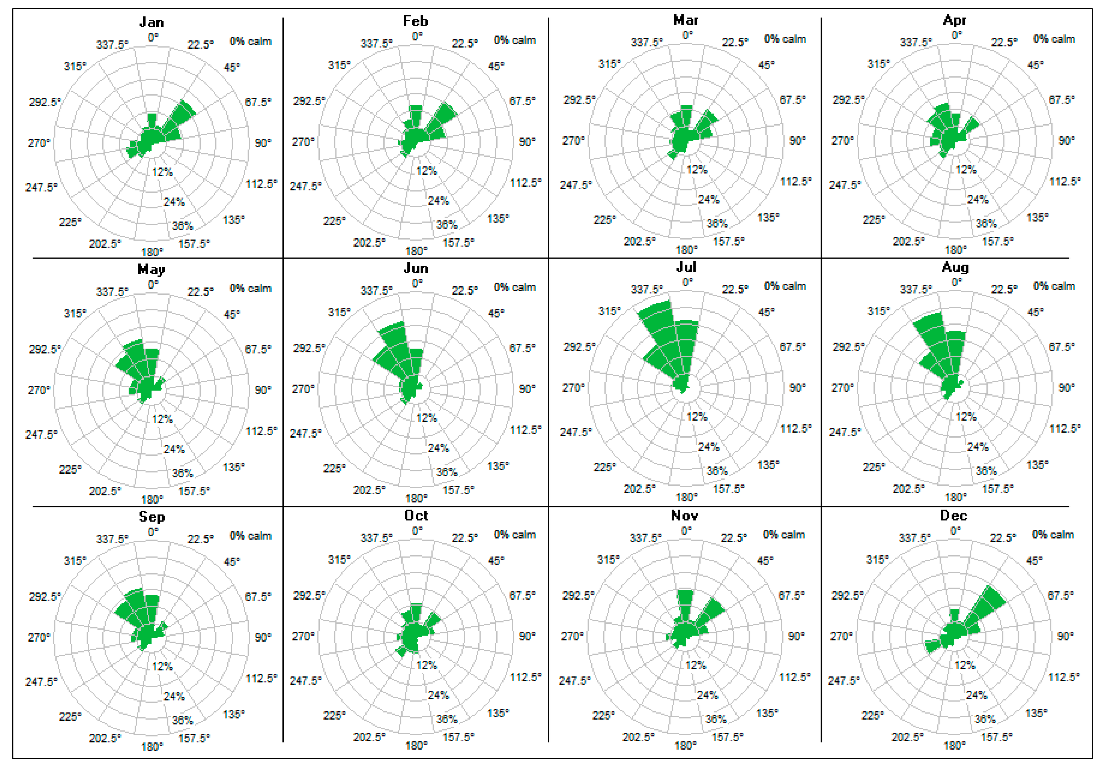
The observation of the monthly wind directions at the Gago Coutinho meteorological station in Figure 6 shows a dominating flow from NNW in summer (JJA), but in the beginning of May (end of spring), the wind becomes more intense and occurs more regularly until the end of summer, known locally as the Nortada regime [5]. During the autumn (SON), winter (DJF), and for half of spring (MA), the winds are highly variable.
The mean diurnal wind speed and the synthesized data for 20 m for each month at Gago Coutinho also show (not shown as figure) the wind speeds are the highest in summer. Constant high wind energy production in autumn and winter cannot be expected, because of the low wind speeds during those seasons. The highest velocities are present mostly in the late afternoon, from April to September.
3.2. The Griggs-Putnam Index of Tree Deformations in Urban Areas (Inside ULisboa Neighborhood)
Inside the urban fabric it is very difficult to evaluate the components of wind with precision, due to urban elements and turbulence. In order to access wind potential in the streets, a methodological approach using a bioindicator is presented in this section. The G-PID is generally used in open terrains, but never in urban areas. It would be interesting if the use of this index could be applied in future wind power assessments. This section presents a detailed evaluation inside the micrometeorological area to demonstrate the effectiveness of this method.
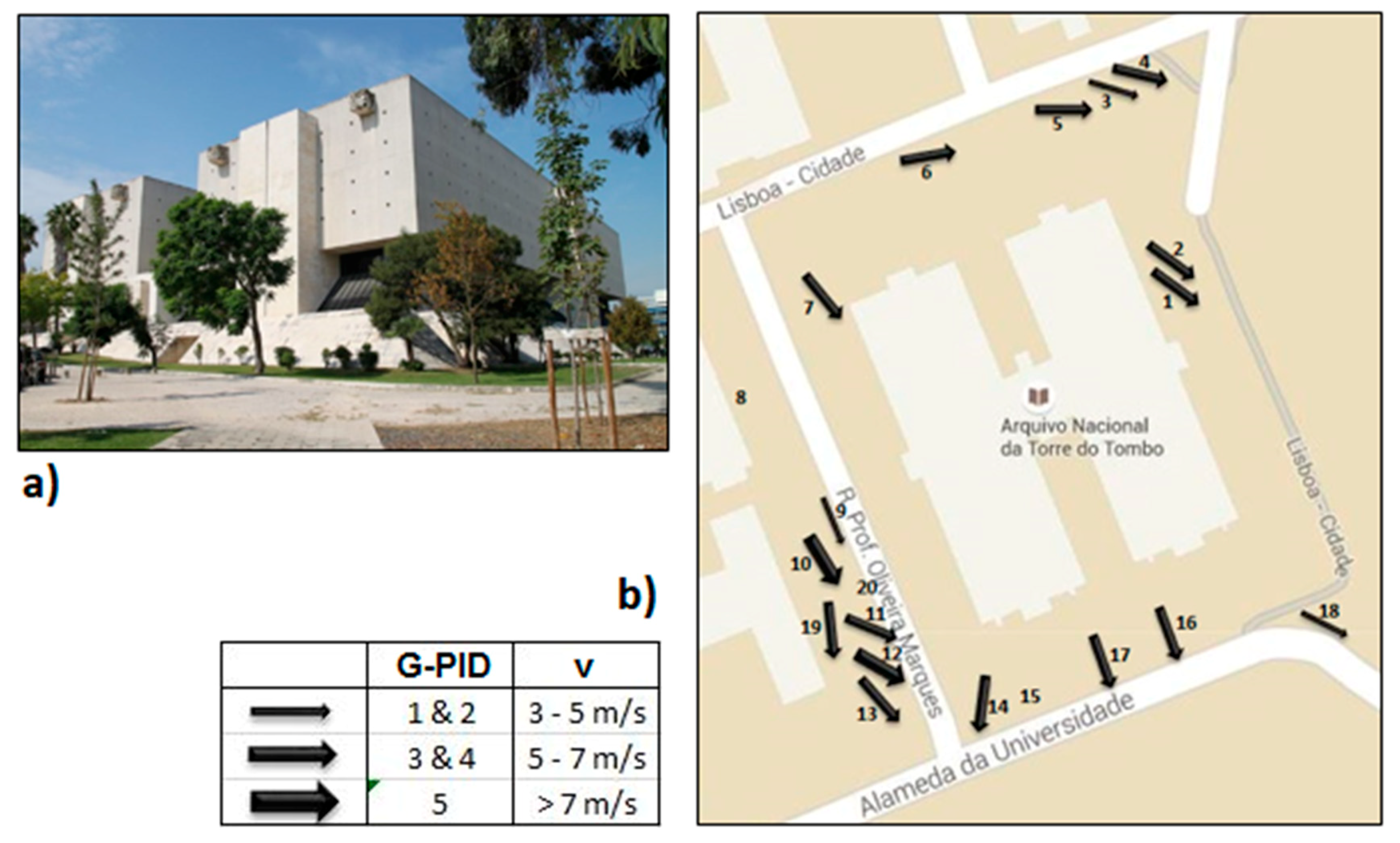
Some clearly wind-deformed trees (coniferous and broadleaf trees) in the neighborhood of the main campus of the University of Lisbon (around the “Arquivo Nacional da Torre do Tombo/Portuguese Historical Arquive”), were chosen, and the G-PID was computed (Figure 7). In Table 3, the observed trees characteristics, with a globose and conic shaped crown around the building area, are presented:
From the survey (Table 3), all trees showed a deformation with the wind direction, and were bent to S and SE (Figure 7); this is consistent with the meteorological data of Gago Coutinho (see Figure 6 from April until September, including the strongest wind conditions in summer (JJA)). The mean G-PID for all trees is ~3. In the G-PID table presented previously (Table 1, Section 2.3), this value represented an estimated wind speed, which impacted all trees throughout their lifetimes: on average, about 5–6 m/s with a mean tree height of 6 m, excluding the rejected trees marked in red in Table 3.
3.3. Micro-Meteorological (ENVI-Met) Wind Flow Assessment (Inside ULisboa Neighborhood)
In order to validate the results obtained in the prior section, a micrometeorological method based on a CFD model was applied to the same area as that of the G-PID method to simulate wind conditions in the same neighborhood at the Lisbon University campus (Figure 7).
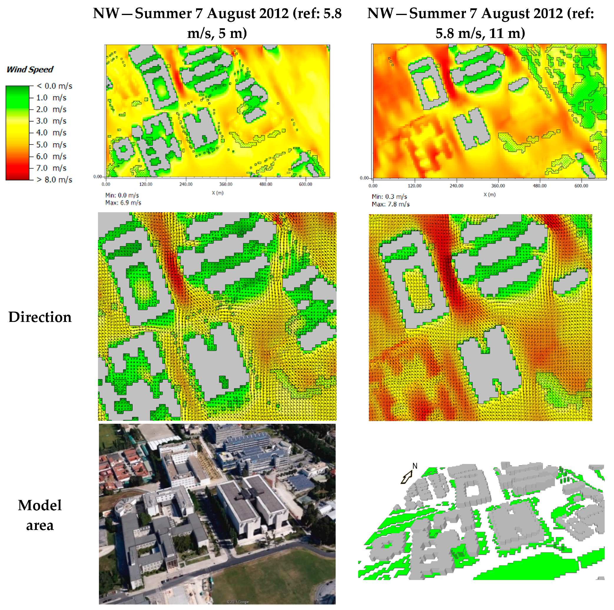
Figure 8 and Table 4 present the results of the micrometeorological simulations and the model area. The table shows all extracted values for every observed tree for spring and summer, while Figure 8 shows only the summer results at 5 and 11 m, since these are the relevant heights that cover the tree shapes, thus giving information about tree deformation by wind speeds and directions during the season with the strongest wind conditions. Comparing the wind directions with Figure 7, similar flow patterns are noticed. Also, wind channeling effects are shown in street canyons around the “Arquivo Nacional da Torre do Tombo”, with wind speeds greater than 6 m/s, that show the strong wind activity during that season. In general, the ENVI-met wind speeds around the H-shaped building (where the observed trees are located) are between 3–6 m/s at 5 m height and 4–7 m/s at 11 m. These values show similar patterns to those in the field work with bioindicators, where a mean wind speed of 5–6 m/s for a mean tree height of 6 m (tree heights vary from 3.3–10 m) was observed.
Table 4 also shows the G-PID mean wind speed (e.g., index class 3 has a wind speed of 5–6 m/s (Table 1). The mean of this is 5.5 m/s), which is much higher in comparison to the modeling results at the lower levels of 5 or 11 m. The 15 m ENVI-met and the summer wind results fit best to the G-PID. This will be further discussed in Section 4.
3.4. WAsP Local Wind Power Assessment
As mentioned in Section 2.4.2, the boundary conditions for WAsP modeling were based on a hypothetical installation of a Skystream 3.7 wind turbine that has a cut-in wind speed of about 3.5 m/s (the wind speed at which the turbine starts to rotate and generates usable power), and a rated wind speed of 13 m/s (when the power output reaches the upper limit) [42].
The Skystream 3.7 has a cut-out speed of 25 m/s, i.e., the maximum wind speed at which the turbine is allowed to deliver power before shutdown, and a survival speed of 63 m/s. An attempt was made to assess such extreme wind for the period from 1984 and 2013 at the Gago Coutinho meteorological station. Over this 30 years period, a maximum of 18.3 m/s was registered. Wind speeds between 10 m/s and 15 m/s had the highest cumulative probability of about 60 %. They represent the class of extreme wind speeds that appeared most frequently. Based on this data, we expect no serious danger (e.g., damages) in the future for a skystream 3.7 turbine.
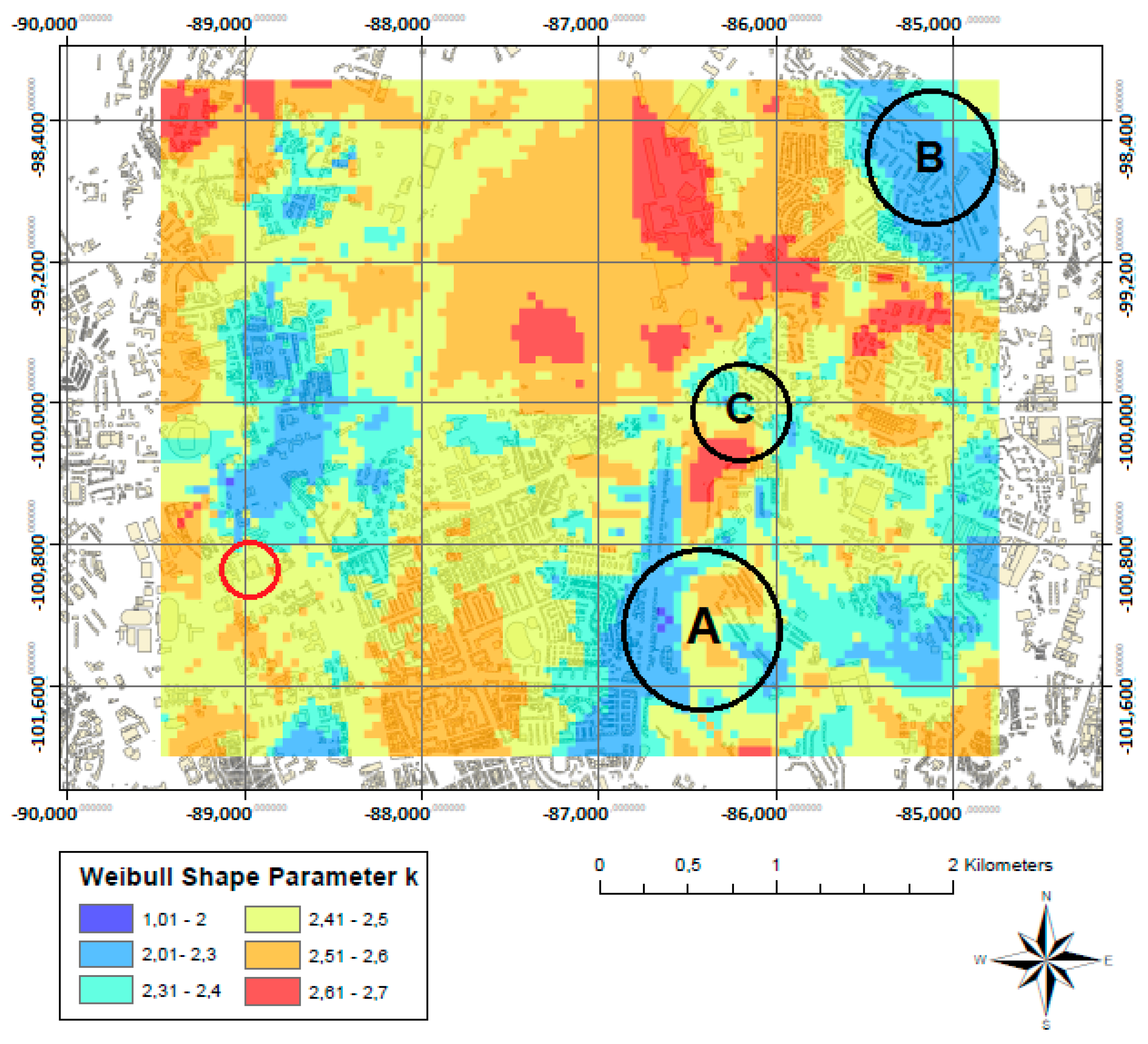
From the estimated mean wind speed map (Figure 9), it is possible to assess the areas with good wind power potential. Also, the Weibull shape parameter k, which shows the variability of the wind speed, shows constant appearance of different wind speeds in nearly every open space (Figure 10). This result is essential for wind power assessment, because constant wind is a good indicator for potential. Possible energy output for the turbine installations would be very problematic to calculate with variable wind speeds and directions. This issue is not treated here.
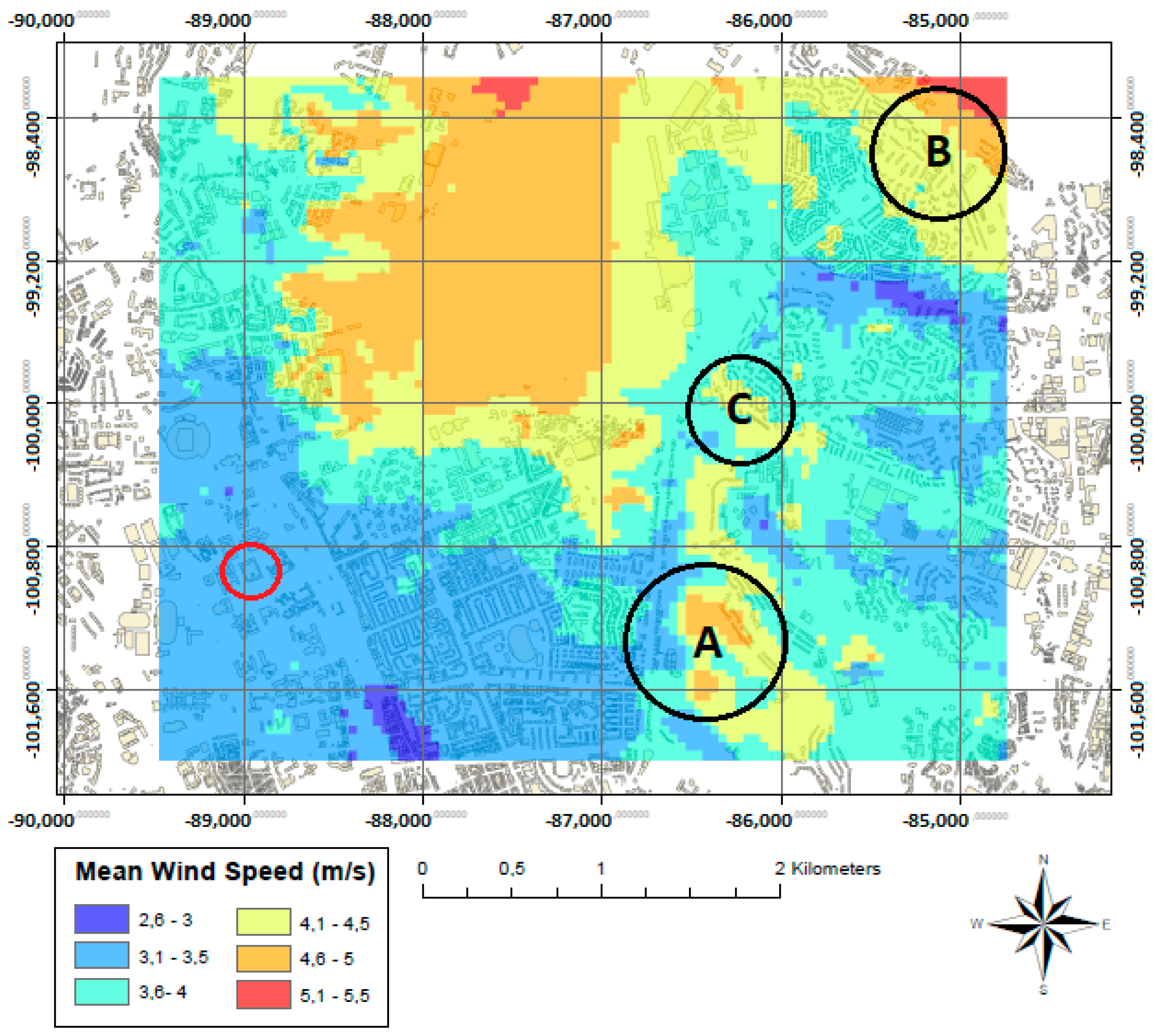
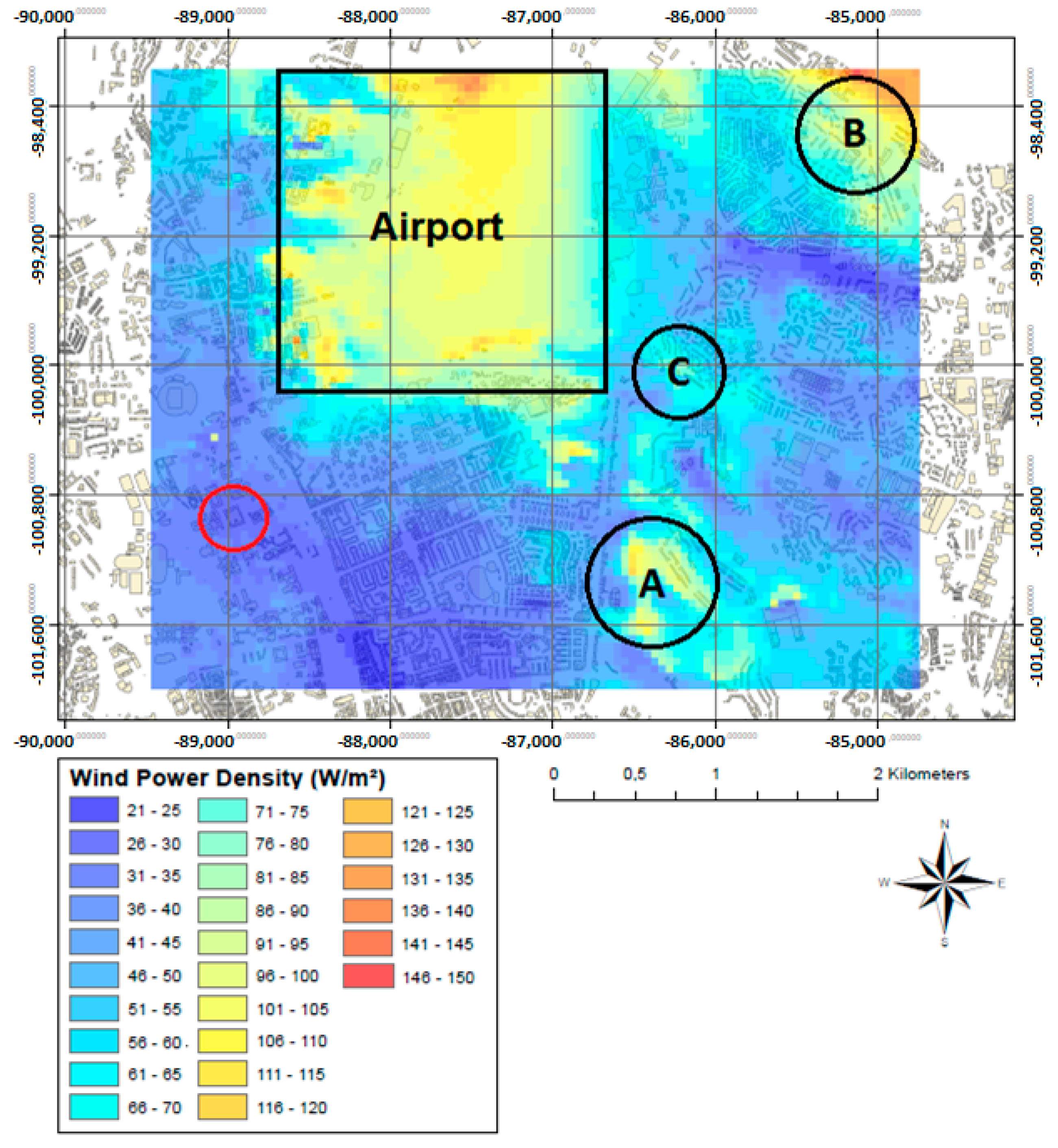
The wind power density in the northern part of Lisbon is presented in Figure 11. Three areas with good wind power potential are marked as A, B, and C. As shown Figure 9, Figure 10 and Figure 11, place “A” has a high k value (2.5–2.6), a mean speed of about 4–5 m/s, and a power density of between ~90 and 115 W/m2. Two other areas with good wind power potential are marked in the map as well. Area “B” shows a k value of between 2.0 and 2.3, mean wind speeds of 4.1–4.5 m/s, and power density of between ~90 and 115 W/m2. Area “C” also has a high k value (~2.4), mean wind speeds of approximately 4.2 m/s, and a power density of between ~70 and 95 W/m2. The Lisbon Airport runways (big yellow area) are excluded in this analysis for obvious reasons, but the results can be interesting, especially if the planned relocation of this infrastructure occurs in the next years, or if the data is transposed to new neighborhoods in the region with similar wind conditions. In the microclimatic area (B in Figure 1, and the red circle in Figure 9, Figure 10 and Figure 11), the estimated wind speed is about 3.1–3.5 m/s, and the wind power potential is about 20 to 40 W/m2. This result is about 2–3 m/s lower than the aforementioned G-PID mean wind speed of 5–6 m/s.
The WAsP simulations were produced after the field work (bioindicators/G-PID) at ULisboa. Further tree observation attempts (G-PID calculations) at locations A, B, and C would make for an interesting comparison to the results of the G-PID of this study, for validation purposes.
4. Discussion
In this section, a discussion of the results concerning the research of tree deformation by wind, in comparison with ENVI-met and WAsP simulations, is presented.
The aforementioned result of the G-PID of 5–6 m/s (Section 3.2) in the G-PID research area ULisboa is about 2–3 m/s higher than the WAsP annual estimation/average from Figure 9 (Section 3.4), all directions included; this can be attributed to the fact that strongest winds occur during the growing seasons in spring and summer (see Section 2.1 and Section 3.1), contributing mainly to the tree deformations, and therefore, representing the higher wind speeds shown in the G-PID results.
According to the WAsP wind speed map (Figure 9), an annual mean between 3.1 and 3.5 m/s at 16 m height is presented around the “Arquivo Nacional da Torre do Tombo” (G-PID research area). Comparing these values with the 15 m ENVI-met simulation, the area shows a mean summer wind speed of approximately ~5.8 m/s (Table 4), and is therefore ~2.3 to 2.7 m/s higher than the results of the WAsP simulation. For the ENVI-met spring mean value of 4.6 m/s, the difference to the aforementioned annual WAsP mean wind speed is ~1.1 to 1.5 m/s. These deviations can be explained by differences between the two models: WAsP calculates an annual average wind speed over the whole period (from 2003 to 2013) at the local scale, whereas ENVI-met reproduced typical summer and spring conditions at the micrometeorological scale with much higher resolution, i.e., when the aforementioned “Nortada” wind regime was more intense (see Section 2.4.2 for more information about the differences between the models).
The results of ENVI-met in Table 4 show, in general, that the summer values are higher than those of spring, as was pointed out before. On average, the differences between those seasons amount to ~1 m/s respectively for each height, which is generally consistent with observations (Figure 5). This leads to the conclusion that the difference between the spring wind speeds from ENVI-met and the G-PID values is too high for a representative comparison; this means that the future focus will be put on the summer statistics of ENVI-met, which fit better as comparisons to the G-PID.
The calculated wind speed averages for G-PID (Table 4) are 6.4 m/s for globose and 4.8 m/s for conic trees (mean = 5.9 m/s). By comparing the mean value in brackets with the average ENVI-met summer wind speeds of 3.6 m/s (at 5 m height) and 4.9 m/s (at 11 m height), we obtain differences of 2.3 m/s and 1 m/s, respectively. The difference at 5 m is slightly high, but at 11 m it is less significant. As mentioned before, the tree alignments in the streets vary from 3.3 m up to 10 m, with a mean height of 6 m (Table 3). Therefore, most deformations respond better with increasing high winds. In addition, the ENVI-met values start matching the G-PID values with increasing height.
One explanation for the deviation between the G-PID and ENVI-met (especially at 5 m) could be inaccuracies while creating the model area for the ENVI-met simulation; it was hardly possible to recreate reality to 100% accuracy in the model area (every grid cell gets filled with an attribute (building, vegetation or soil) according to a bird’s eye view image. In that sense, buildings, trees, and soils were sometimes impossible to reproduce with diagonal/smooth edges, leading to step formations (Figure 8, picture bottom right, grey spaces). Also, trunk thickness is an important factor that defines the stability of a tree. The thicker the trunk, the more the tree will resist strong wind speeds. For trees with narrow trunks, even slow winds could be very cause deformation. The much slower wind speeds of the ENVI-met simulation could be strong enough to deform the trees with a slim trunk, of which a lot are present in the research area. In future, this effect should be taken into account. Another important explanation is the fact that the simulation took place in an urban area, where wind speed is slowed down by urban structures (although in some places, accelerations can take place, due to the well-known Venturi effect) (Figure 8).
Furthermore, most of the studies with bioindicators where tested in non-urban areas. Wooldridge et al. [43] observed wind speed and direction through deformation indices and other methods in a small subalpine basin of Southern Wyoming (USA). They focused on single trees, where no other obstacles could be found, and obtained normal Index values without deviation. Robertson [44] focused on Newfoundland, as well on isolated trees, and only one species; under these conditions, the same results were obtained.
This leads us to make attempts to correct the values of the estimated wind speeds from ENVI-met with tree deformations. A possible modification of the G-PID could take the following form: since the 5 m and 11 m ENVI-met simulations cover tree shapes, and the best wind conditions for tree deformation occur in summer, an average of both summer mean wind speeds at these heights, including all trees, can be calculated (3.6 m/s + 4.9 m/s; see Table 4), giving ~4.25 m/s. The deviation between the G-PID average wind speed for all trees (Table 4; see Section 3.3 for an explanation), 5.9 m/s, and the just calculated 4.25 m/s, is then 1.7 m/s (≈2 m/s). This value would be the modification factor for the G-PID, and can be subtracted from every wind speed class, as shown in Figure 12 (only indexes from 0 to 5 are presented, because this corresponds to the observation in the area). Since the G-PID was only used for open terrains, and not in urban areas, this is consistent with previous works [5], where a decrease of up to 30% on average wind speeds was estimated in Lisbon due to urbanization. As well comparing the ENVI-met mean summer wind speed of 4.9 m/s at 11 m with observations of about 3.6 m/s at measuring height (10 m), and taking into account that the observation data is measured near the airport where much lower roughness is given than for the model area (urban structure), it can be assumed that the results of ENVI-met are representative as a comparison to the G-PID, what further supports the calculated modification of about 2 m/s.
We think this modification of the G-PID could be very useful for future wind power assessments using trees in urban spaces, although much more research must be done to confirm these results.
5. Conclusions
This study was focused on testing an approved method for non-urban areas (G-PID), coupled with linearized and CFD models, to assess wind power potential in the northern part of Lisbon.
With the WAsP model, it was possible to locate three potential areas for a Skystream 3.7 installation that would generate autonomous energy for households and public institutions. Additionally, according to the observation data at Gago Coutinho, the highest energy potential would be in the late afternoon (5 p.m. = strongest wind conditions) from April to September, but especially during the summer (JJA).
It was necessary to adapt the G-PID to urban wind power assessment with the help of the wind flow model, ENVI-met. In a first attempt, a new scheme for the visual assessment of wind conditions in urban areas was made. A reduction value of about 2 m/s was found to be a viable modification factor.
However, we recommended further studies with the G-PID in other street canyons of Lisbon (or other cities with similar wind conditions), with a sufficient number of trees, for comparison. Also, the tree species and characteristics should be taken into account. We assume that this is one of the main limitations in this research, because the deformation of trees depends not only on the prevailing winds and the exposure of the tree, but also on the tree species and local phytosanitary conditions [43,46], which were not taken into account. However, the statistical results prove that, at least in the study area, the results are in agreement with previous research [5]. It could also be very interesting to use other CFD software, such as the aforementioned “OpenFOAM” and “ANSYS Fluent”, for future comparisons with the G-PID, and finally, for validation of the “ENVI-met” results presented in this study. Also, an “ENVI-met” simulation with a higher resolution would be of great benefit since the model is still under development.
In conclusion, this study showed helpful results with interesting potential for future research, but remains a first approach, and requires more investigation.
Acknowledgments
First of all, I would like to thank António Lopes for his support as advisor during my work in Lisbon. In addition, I want to express my gratitude to him and Andreas Matzarakis for all their support as writing assistance and proof readers. And finally I send my appreciation to Flávio Mendes and Elis Alves for their help during my research in Lisbon.
Conflicts of Interest
There exist no conflicts of interest and therefore no financial/personal interest or belief that could affect the objectivity of the submitted research paper.
References
- Kaltschmitt, M.; Streicher, W.; Wiese, A. Renewable Energy. In Technology, Economics and Environment; Springer: Berlin/Heidelberg, Germany; New York, NY, USA, 2007; ISBN 978-3-540-70947-3. [Google Scholar]
- Turner, J.A. A Realizable Renewable Energy Future. Science 1999, 285, 687–689. [Google Scholar] [CrossRef] [PubMed]
- Newman, P.W.G. Sustainability and cities: Extending the metabolism model. Lands. Urban Plan. 1999, 44, 219–226. [Google Scholar] [CrossRef]
- Alcoforado, M.J.; Andrade, H.; Lopes, A.; Vasconcelos, J.; Vieira, R. Observational studies on summer winds in Lisbon (Portugal) and their influence on daytime regional and urban thermal patterns. Merhavim 2006, 6, 90–112. [Google Scholar]
- Lopes, A.; Saraiva, J.; Alcoforado, M.J. Urban boundary layer wind speed reduction in summer due to urban growth and environmental consequences in Lisbon. Environ. Model. Softw. 2011, 26, 241–243. [Google Scholar] [CrossRef]
- Häckel, H. Meteorologie, 7th ed.; UTB Verlag Stuttgart: Stuttgart, Germany, 2012; ISBN 13 978-3825237004. [Google Scholar]
- American Wind Energy Association (AWEA). In the Public Interest. How and Why to Permit for Small Wind Systems. In A Guide for State and Local Governments; AWEA: Washington, DC, USA, 2008. [Google Scholar]
- Krohn, S.; Damborg, S. On Public Attitudes towards Wind Power. Renew. Energy 1999, 16, 954–960. [Google Scholar] [CrossRef]
- Lopes, A.; Correia, E. A proposal to enhance urban climate maps with the assessment of wind power potential. The case of Cascais Municipality (Portugal). In Proceedings of the BIOCLIMATE 2012, “Bioclimatology of Ecosystems” International Scientific Conference, Ústí nad Labem, Czech Republic, 29–31 August 2012; pp. 68–69, ISBN 978-80-213-2299-8. [Google Scholar]
- Berge, E.; Gravdahl, A.R.; Schelling, J.; Tallhaug, L.; Undheim, O. Wind in Complex Terrain. A Comparison of WAsP and Two CFD-Models; Kjeller Vindteknikk AS: Gunnar Randers Vei, Norway, 2006. [Google Scholar]
- Simões, T.; Estanqueiro, A. A new methodology for urban wind resource assessment. Renew. Energy 2016, 89, 598–605. [Google Scholar] [CrossRef] [Green Version]
- Acker, T.; Chime, A.H. Wind Modeling Using WindPro and WAsP Software; Sustainable Energy Solution Lab, Mechanical Engineering Department, Northern Arizona University: Flagstaff, AZ, USA, 2011; pp. 1–11. [Google Scholar]
- Cullen, S. Trees and wind: Wind scales and speeds. J. Arboric. 2002, 28, 237–242. [Google Scholar]
- Wade, J.E.; Hewson, E.W. Trees as a Local Climatic Wind Indicator. J. Appl. Meteorol. 1979, 18, 1182–1187. [Google Scholar] [CrossRef] [Green Version]
- Putnam, P.C. Power from the Wind; Van Nostrand-Reinhold: Princeton, NJ, USA, 1948; 223p. [Google Scholar]
- Yoshino, M.M. Studies of wind-shaped trees: Their classification, distribution and significance as a climatic indicator. Climatol. Notes 1973, 12, 1–52. [Google Scholar]
- Hewson, E.W.; Wade, J.E.; Baker, R.W. A Handbook on the Use of Trees as an Indicator of Wind Power Potential; Final Report; Oregon State University: Corvallis, OR, USA, 1979. [Google Scholar]
- Sagrillo, M. Site Analysis for Wind Generators. Part 1: Average Wind Speed. Home Power 1994, 40, 86–90. [Google Scholar]
- Sagrillo, M. Site Analysis for Wind Generators. Part 2: Your Site. Home Power 1994, 41, 60–65. [Google Scholar]
- Mattio, H.F.; Ponce, G.A. Nociones Generales de Energía Eólica; National University of Salta: Salta, Argentina, 1998; pp. 159–167. [Google Scholar]
- Meneses, B.; Lopes, A. An integrated approach for wind fields assessment in coastal areas, based on bioindicators, CFD modeling, and observations. Theor. Appl. Climatol. 2015, 128, 301–310. [Google Scholar] [CrossRef]
- Bruse, M.; Fleer, H. Simulating surface- plant-air interactions inside urban environments with a three dimensional numerical model. Environ. Softw. Model. 1998, 13, 373–384. [Google Scholar] [CrossRef]
- Correia, E.; Lopes, A.; Marques, D. An automatic GIS procedure to calculate urban densities to use in Urban Climatic Maps. In Proceedings of the 9th International Conference on Urban Climate, 12th Symposium on the Urban Environment, Toulouse, France, 20–24 July 2015. [Google Scholar]
- Portugal, INE. Censos 2011 Resultados Definitivos—Portugal; Statistics Portugal; Instituto Nacional de Estatística: Lisboa, Portugal, 2012.
- Lopes, A.; Alves, E.; Alcoforado, M.J.; Machete, R. Lisbon Urban Heat Island Updated: New Highlights about the Relationships between Thermal Patterns and Wind Regimes. Adv. Meteorol. 2013, 2013, 487695. [Google Scholar] [CrossRef]
- Freire, P.; Andrade, C. Wind-induced sand transport in Tagus estuarine beaches. Aquat. Ecol. 1999, 33, 225–233. [Google Scholar] [CrossRef]
- Borrego, C.; Tchepel, O.; Costa, A.M.; Amorim, J.H.; Miranda, A.I. Emission and dispersion modelling of Lisbon air quality at local scale. Atmos. Environ. 2003, 37, 5197–5205. [Google Scholar] [CrossRef]
- Alcoforado, M.J.; Lopes, A.; Alves, E.; Canário, P. Lisbon heat Island statistical study (2004-2012). Finisterra 2014, 49, 61–80. [Google Scholar] [CrossRef]
- Mayer, H. Baumschwingungen und Sturmgefährdung des Waldes; Münchener Universitäts-Schriften, Meteorologisches Institut: Munich, Germany, 1985; Volume 51, pp. 99–111. [Google Scholar]
- Amtmann, R. Dynamische Windbelastung von Nadelbäumen. In Forstliche Forschungsberichte München; Forstwissenschaftlichen Fakultät der Universität München: Munich, Germany, 1986; Volume 74, p. 52. [Google Scholar]
- Lopes, A.; Oliveira, S.; Fragoso, M.; Andrade, J.; Pedro, P. Wind risk assessment in urban environments: The case of falling trees during windstorm events in Lisbon. In Bioclimatology and Natural Hazards; Střelcová, K., Mátyás, C., Kleidon, L., Lapin, M., Matejka, F., Blaženec, M., Škvarenina, J., Holécy, J., Eds.; Springer: Dordrecht, The Netherlands, 2008; pp. 55–74. [Google Scholar] [CrossRef]
- Manwell, J.F.; McGowan, J.G.; Rogers, A.L. Wind Energy Explained. In Theory, Design and Application, 2nd ed.; WILEY: Chichester, UK, 2009; ISBN 978-0-470-01500-1. [Google Scholar]
- Hiester, T.R.; Pennell, W.T. The Meteorological Aspects of Siting Large Wind Turbines; PNL-2522; Pacific Northwest Laboratory: Richland, WA, USA, 1981. [Google Scholar]
- Blocken, B. 50 years of Computational Wind Engineering: Past, present and future. J. Wind Eng. Ind. Aerodyn. 2014, 129, 69–102. [Google Scholar] [CrossRef]
- Murakami, S. Overview of turbulence models applied in CWE-1997. J. Wind Eng. Ind. Aerodyn. 1998, 74–76, 1–24. [Google Scholar] [CrossRef]
- Lysenko, D.A.; Ertesvag, S.; Rian, K.E. Modeling of turbulent separated flows using OpenFOAM. Comput. Fluids 2013, 80, 408–422. [Google Scholar] [CrossRef]
- Robertson, E.; Choudhury, V.; Bhushan, S.; Walters, D.K. Validation of OpenFOAM numerical methods and turbulence models for incompressible bluff body flows. Comput. Fluids 2015, 123, 122–145. [Google Scholar] [CrossRef]
- Kalvig, S.; Manger, E.; Hjertager, B. Comparing different CFD wind turbine modelling approaches with wind tunnel measurements. J. Phys. Conf. Ser. 2014, 555, 012056. [Google Scholar] [CrossRef] [Green Version]
- Huttner, S.; Bruse, M. Numerical modeling of urban climate—A preview on ENVI-met 4.0. In Proceedings of the Seventh International Conference on Urban Climate, Yokohama, Japan, 29 June–3 July 2009. [Google Scholar]
- Baltazar, S. New Bioclimatic Maps of Lisbon. Finisterra 2014, 49, 81–94. [Google Scholar] [CrossRef]
- Elektrotechnik Stevens. Wind Turbine Skystream 3.7. Updated 2018. Available online: http://www.pro-umwelt.de/windturbine-skystream-37-p-802.html?language=en (accessed on 6 January 2016).
- Xzeres Wind. Wind Turbine Skystream 3.7. Updated 2013. Available online: http://www.windenergy.com/products/skystream/skystream-3.7 (accessed on 11 November 2015).
- Wooldridge, G.; Musselman, R.; Connell, B.; Fox, D. Airflow Patterns in a Small Subalpine Basin. Theor. Appl. Climatol. 1992, 45, 37–41. [Google Scholar] [CrossRef]
- Robertson, A. Estimating Mean Windflow in Hilly Terrain from Tamarack (Larix laricina (Du Roi) K. Koch) Deformation. Int. J. Biometeorol. 1986, 30, 333–349. [Google Scholar] [CrossRef]
- Gipe, P. Wind Power. Renewable Energy for Home, Farm, and Business. In Completely Revised and Expanded Edition; Chelsea Green Publishing: Chelsea, VT, USA, 2004; ISBN 9781931498142. [Google Scholar]
- Sellier, D.; Fourcaud, T. Crown structure and wood properties: Influence on tree sway and response to high winds. Am. J. Bot. 2009, 96, 885–896. [Google Scholar] [CrossRef] [PubMed] [Green Version]
Figure 1.
The city of Lisbon and the two study areas: (A) Local scale (3.5 km × 3.5 km); (B) Micrometeorological scale (0.5 km × 0.5 km) around the principal campus of the University of Lisbon.
Figure 1.
The city of Lisbon and the two study areas: (A) Local scale (3.5 km × 3.5 km); (B) Micrometeorological scale (0.5 km × 0.5 km) around the principal campus of the University of Lisbon.

Figure 2.
Urban densities and green spaces in the larger study area (see Figure 1A).
Figure 2.
Urban densities and green spaces in the larger study area (see Figure 1A).

Figure 3.
Wind regimes in spring and summer (the trees growing season) at 10 m. The percentage distribution of Wind directions (°) is shown in gray.
Figure 3.
Wind regimes in spring and summer (the trees growing season) at 10 m. The percentage distribution of Wind directions (°) is shown in gray.

Figure 4.
Measuring the shape and deformation index of trees. Top: Globose tree, Below: Conic tree. A, B and G are the measured parameters that are needed for Equations (1) and (2) (see description below). Z is the tree height.
Figure 4.
Measuring the shape and deformation index of trees. Top: Globose tree, Below: Conic tree. A, B and G are the measured parameters that are needed for Equations (1) and (2) (see description below). Z is the tree height.


Figure 5.
Diurnal wind speed curves at 10 m height for each season (and 20 m height synthesized/extrapolated for Summer) over the ten years period (2003–2013) at Gago Coutinho.
Figure 5.
Diurnal wind speed curves at 10 m height for each season (and 20 m height synthesized/extrapolated for Summer) over the ten years period (2003–2013) at Gago Coutinho.

Figure 6.
Monthly wind directions at 10 m measuring height over the ten-year period from 2003–2013 at Gago Coutinho.
Figure 6.
Monthly wind directions at 10 m measuring height over the ten-year period from 2003–2013 at Gago Coutinho.

Figure 7.
(a) The tree research area (Arquivo Nacional da Torre do Tombo); (b) Arrows describe the direction of deformation through observations, and the intensity of deformation for every observed tree based on the G-PID (Source: Google Maps).
Figure 7.
(a) The tree research area (Arquivo Nacional da Torre do Tombo); (b) Arrows describe the direction of deformation through observations, and the intensity of deformation for every observed tree based on the G-PID (Source: Google Maps).

Figure 8.
ENVI-met micrometeorological simulation of average wind conditions during summer at 5 m and 11 m, at 5 p.m., around the Arquivo Nacional da Torre do Tombo (“H” shaped building in the center). The trees are represented by the green spots around that building (picture top left). The trees could not be implemented exactly. The direction of deformation of the trees (black arrows) are shown in the middle of the figure. The model area is presented at the bottom.

Figure 9.
Annual mean wind speed map (m/s) of the northern part of Lisbon based on 10 years’ (2003–2013) hourly data from Gago Coutinho, created with WAsP and postedited with ArcMap, presenting three locations with wind power potential for the northern part of Lisbon (A, B and C). The red circle symbolizes the research area for the Griggs-Putnam Index in the university area.

Figure 10.
Annual Weibull shape parameter k of the northern part of Lisbon based on 10 years’ (2003–2013) hourly data from Gago Coutinho, created with WAsP and postedited with ArcMap, presenting three locations with wind power potential for the northern part of Lisbon (A, B and C). The red circle symbolizes the research area for the Griggs-Putnam Index in the university area.

Figure 11.
Annual wind power density map (W/m2) of the northern part of Lisbon based on the 10 years’ (2003–2013) hourly data from Gago Coutinho, created with WAsP and postedited with ArcMap, presenting three spots with wind power potential for the northern part of Lisbon (A, B and C). The red circle symbolizes the research area for the Griggs-Putnam Index in the university area.

Figure 12.
The new Index of Deformity. It includes coniferous and broadleaf trees as the original index. The original wind speed classes have been modified to lower levels (“G-PID new: wind speed [m/s]”). Only index classes 0–5 are shown, because higher index classes were non-existent in the research area. As a reference, the “old” index wind speeds are added (“G-PID old: wind speed [m/s]”). Descriptions and Shapes are from Gipe [45] and Hiester and Pennell [33].


Table 1.
G-PID with its classes, related wind speeds, and description [33]. Griggs-Putnam Index of Deformity.
Table 1.
G-PID with its classes, related wind speeds, and description [33]. Griggs-Putnam Index of Deformity.
| Class | Wind Speed [m/s] | Description |
|---|---|---|
| 0 | insignificant wind speed | No Effect: Careful examination of needles, twigs, and branches indicates that the wind has had no noticeable influence on the tree. |
| I | 3–4 | Brushing: The small branches and needles appear bent away from the prevailing wind direction. The tree crown may appear slightly asymmetrical if carefully examined. |
| II | 4–5 | Slight Flagging: The small branches and the ends of the larger branches are bent by the wind, giving the tree a noticeably asymmetric crown. |
| III | 5–6 | Moderate Flagging: The large branches are bent toward the leeward side of the tree, giving the tree a nearly one-sided crown. |
| IV | 6–7 | Strong Flagging: All the branches are swept to the leeward and the trunk is bare on the windward side. The tree resembles a banner. |
| V | 7–8 | Partial Throwing: A partially thrown tree is one in which the trunk, as well as the branches, are bent to the lee. The trunk may be bent in a concave or convex fashion, but rises vertically near the ground and the degree of bending increases near the top of the trunk. |
| VI | 8–9 | Complete Throwing: The tree grows nearly parallel to the ground and along the path of the prevailing wind. The larger branches on the leeward side may extend beyond the tip of the trunk. |
| VII | >10 | Carpeting: The wind is so strong, permanent or accompanying conditions so severe (e.g., ice is present) that the tree takes the form of a shrub. Upright leaders are killed and lateral growth predominates. The crown grows across the ground like a prostrate shrub. |
Table 2.
Metadata, initiation and boundary condition of the micrometeorological model of ULisboa Campus (Arquivo National da Torre do Tombo, Lisboa, Portugal), with ENVI-met in two simulated days: spring 17 May 2012 and summer 7 August 2012).
Table 2.
Metadata, initiation and boundary condition of the micrometeorological model of ULisboa Campus (Arquivo National da Torre do Tombo, Lisboa, Portugal), with ENVI-met in two simulated days: spring 17 May 2012 and summer 7 August 2012).
| Date & Time | 17 of May 2012; 17:00 h | 7 of August 2012; 17:00 h |
|---|---|---|
| Wind speed (m/s)/direction (°) (10m) 1 | 4.9/340 | 5.8/330 |
| Initial potential temperature (K) 2 | θ = 293.5 | θ = 302.5 |
| Relative Humidity (2 m) (%) 3 | 73 | 48 |
| Specific Humidity (2500 m) (g water/kg air) 4 | q = 2.8 | q = 3.5 |
| Location (φ, λ, alt)/Köppen Class | 38°45′ N, 9°10′ W, ≈87 m/Csa | |
| Model horizontal area (a) | ≈2500 | |
| Grid size (x,y,z) dx, dy, dz (m) | 140 × 80 × 20 4.8 × 4.8 × 2 | |
| Roughness length (z0) at the Gago Coutinho meteorological station (m) (Complementary to the Wind Speed. Defines the surface roughness at the location, where the wind speed in 10 m was measured. Both values are used to calculate the geostrophic wind. Not further used after initialization.) | 0.1 | |
Sources: 1, 2 and 3: IPMA (distributed by NOAA/NCDC-Climate Data Online [https://gis.ncdc.noaa.gov]; 4: NOAA/ESRL Vertical Profiles of Reanalysis Datasets [http://www.esrl.noaa.gov/psd/map/profile/].
Table 3.
Globosely and conic (bold) shaped trees with species name, geographic orientation within the study area, and the measured variables (A, B, G) needed for the calculation of the G-PID by Equations (1) and (2). The height of the reference person in the picture is needed for converting the manually measured values from cm into m. Trees marked in red were rejected (see Section 2.3).
| Tree Number | Species | Geographic Direction Taking the Perspective from the Building Center (Azimuth in Degrees) | ||||||||||
|---|---|---|---|---|---|---|---|---|---|---|---|---|
| 1 | Quercus robur (British oak) | 45.90 | ||||||||||
| 2 | Quercus robur (British oak) | 39.04 | ||||||||||
| 3 | Prunus cerasifera (Cherry plum) | 11.64 | ||||||||||
| 4 | Prunus cerasifera (Cherry plum) | 14.76 | ||||||||||
| 5 | Acacia longifolia (Long leaf acacia) | 3.14 | ||||||||||
| 6 | Olea europaea (Olive tree) | 339.76 | ||||||||||
| 7 | Acacia longifolia (Long leaf acacia) | 299.05 | ||||||||||
| 8 | Fraxinus sp (Ash) | 274.19 | ||||||||||
| 9 | Populus sp (Poplar) | 235.53 | ||||||||||
| 10 | Prunus cerasifera (Cherry plum) | 228.96 | ||||||||||
| 11 | Prunus cerasifera (Cherry plum) | 209.54 | ||||||||||
| 12 | Prunus cerasifera (Cherry plum) | 203.99 | ||||||||||
| 13 | Morus alba (White mulberry) | 202.05 | ||||||||||
| 14 | Jacaranda mimosifolia (Palisander) | 189.17 | ||||||||||
| 15 | Jacaranda mimosifolia (Palisander) | 181.87 | ||||||||||
| 16 | Jacaranda mimosifolia (Palisander) | 147.74 | ||||||||||
| 17 | Jacaranda mimosifolia (Palisander) | 162.95 | ||||||||||
| 18 | Grevillea robusta (Australian silver oak) | 127.02 | ||||||||||
| 19 | Casuarina equisetifolia (Horsetail she oak) | 216.19 | ||||||||||
| 20 | Cercis siliquastrum (Judas tree) | 219.49 | ||||||||||
| Tree Number (globose) | Tree height (cm) | Tree height (m) | A (cm) | B (cm) | G (degree) | Height of reference person in picture (cm) | Height of reference person in reality (m) | A (m) | B (m) | G (radian) | G-PID | Final G-PID (rounded) |
| 1 | 8.93 | 6.11 | 4.90 | 1.70 | 42.39 | 2.50 | 1.71 | 3.35 | 1.16 | 0.74 | 3.82 | 4 |
| 2 | 8.90 | 7.25 | 5.50 | 2.00 | 45.56 | 2.10 | 4.48 | 1.63 | 0.80 | 3.76 | 4 | |
| 4 | 9.95 | 5.87 | 7.50 | 4.40 | 47.50 | 2.90 | 4.42 | 2.59 | 0.83 | 2.76 | 3 | |
| 6 | 9.59 | 3.28 | 7.80 | 3.50 | 67.95 | 5.00 | 2.67 | 1.20 | 1.19 | 3.74 | 4 | |
| 8 | 14.88 | 12.72 | 10.40 | 2.40 | 58.16 | 2.00 | 8.89 | 2.05 | 1.02 | 5.63 | 6 | |
| 10 | 11.08 | 4.21 | 4.30 | 1.00 | 22.91 | 4.50 | 1.63 | 0.38 | 0.40 | 4.81 | 5 | |
| 11 | 11.95 | 5.24 | 4.00 | 1.70 | 27.27 | 3.90 | 1.75 | 0.75 | 0.48 | 2.96 | 3 | |
| 12 | 8.43 | 5.15 | 3.40 | 0.80 | 29.61 | 2.80 | 2.08 | 0.49 | 0.52 | 4.91 | 5 | |
| 13 | 11.42 | 4.07 | 6.50 | 2.30 | 46.14 | 4.80 | 2.32 | 0.82 | 0.81 | 3.85 | 4 | |
| 14 | 10.42 | 4.57 | 6.60 | 2.40 | 46.61 | 3.90 | 2.89 | 1.05 | 0.81 | 3.79 | 4 | |
| 15 | 9.42 | 6.71 | 4.90 | 0.50 | 48.60 | 2.40 | 3.49 | 0.36 | 0.85 | 10.88 | 11 | |
| 16 | 11.64 | 8.29 | 6.50 | 2.30 | 67.79 | 2.40 | 4.63 | 1.64 | 1.18 | 4.33 | 4 | |
| 17 | 6.04 | 7.38 | 3.90 | 2.20 | 56.64 | 1.40 | 4.76 | 2.69 | 0.99 | 3.03 | 3 | |
| 20 | 9.01 | 3.67 | - | - | - | 4.20 | - | - | - | - | - | |
| Tree Number (conic) | Tree height (cm) | Tree height (m) | A (degree) | B (degree) | G (degree) | Height of reference person in picture (cm) | Height of reference person in reality (m) | A (radian) | B (radian) | G (radian) | G-PID | Final G-PID (rounded) |
| 3 | 5.72 | 4.66 | 67.85 | 33.80 | 19.26 | 2.10 | 1.71 | 1.18 | 0.59 | 0.34 | 2.44 | 2 |
| 5 | 13.08 | 7.99 | 34.71 | 14.39 | 9.47 | 2.80 | 0.61 | 0.25 | 0.17 | 2.62 | 3 | |
| 7 | 11.40 | 7.80 | 43.12 | 18.09 | 20.16 | 2.50 | 0.75 | 0.32 | 0.35 | 2.83 | 3 | |
| 9 | 11.30 | 4.60 | 24.64 | 25.20 | 6.14 | 4.20 | 0.43 | 0.44 | 0.11 | 1.11 | 1 | |
| 18 | 9.82 | 5.60 | 33.93 | 16.83 | 15.16 | 3.00 | 0.59 | 0.29 | 0.26 | 2.35 | 2 | |
| 19 | 10.87 | 9.78 | 31.61 | 11.96 | 4.15 | 1.90 | 0.55 | 0.21 | 0.07 | 2.74 | 3 | |
Table 4.
Results of the ENVI-met micrometeorological simulations of average wind conditions during spring and summer at 5 m, 11 m and 15 m, at 5 p.m, around the Arquivo Nacional da Torre do Tombo at each tree location. The G-PID mean wind speeds are also shown.
Table 4.
Results of the ENVI-met micrometeorological simulations of average wind conditions during spring and summer at 5 m, 11 m and 15 m, at 5 p.m, around the Arquivo Nacional da Torre do Tombo at each tree location. The G-PID mean wind speeds are also shown.
| Tree Number | Species | ENVI-Met Simulations Results at the Three Height Levels (m) | G-PID (m/s) | ||||||
|---|---|---|---|---|---|---|---|---|---|
| 5 m | 11 m | 15 m | |||||||
| Spring (m/s) | Summer (m/s) | Spring (m/s) | Summer (m/s) | Spring (m/s) | Summer (m/s) | ||||
| globose | 1 | Quercus robur (British oak) | 2.9 | 3.4 | 3.7 | 4.7 | 4.3 | 5.7 | 6.5 |
| 2 | Quercus robur (British oak) | 3.1 | 3.7 | 3.8 | 5 | 4.4 | 5.8 | 6.5 | |
| 4 | Prunus cerasifera (Cherry plum) | 1.2 | 2 | 2.3 | 3.2 | 3.1 | 4.3 | 5.5 | |
| 6 | Olea europaea (Olive tree) | 3.1 | 3.2 | 3.8 | 6 | 5.1 | 6.8 | 6.5 | |
| 10 | Prunus cerasifera (Cherry plum) | 3.9 | 5.1 | 4.7 | 5.9 | 5.2 | 6.5 | 7.5 | |
| 11 | Prunus cerasifera (Cherry plum) | 3.2 | 4.2 | 4.7 | 5.5 | 5.1 | 6.6 | 5.5 | |
| 12 | Prunus cerasifera (Cherry plum) | 3.2 | 4.5 | 4.7 | 5.8 | 5.2 | 6.6 | 7.5 | |
| 13 | Morus alba (White mulberry) | 3.7 | 4.4 | 4.4 | 5.8 | 5.2 | 6.7 | 6.5 | |
| 14 | Jacaranda mimosifolia (Palisander) | 3.4 | 4.2 | 4.3 | 5.5 | 5 | 6.4 | 6.5 | |
| 16 | Jacaranda mimosifolia (Palisander) | 2 | 3 | 3.1 | 4 | 4.7 | 5.2 | 6.5 | |
| 17 | Jacaranda mimosifolia (Palisander) | 1.9 | 2.9 | 3.1 | 4 | 4.4 | 5.2 | 5.5 | |
| conic | 3 | Prunus cerasifera (Cherry plum) | 1.8 | 2.6 | 2.3 | 3 | 3.1 | 4.6 | 4.5 |
| 5 | Acacia longifolia (Long leaf acacia) | 1.8 | 3 | 2.8 | 4.2 | 3.5 | 5.4 | 5.5 | |
| 7 | Acacia longifolia (Long leaf acacia) | 2.6 | 3.2 | 4 | 4.4 | 4.8 | 5.4 | 5.5 | |
| 9 | Populus sp (Poplar) | 2.6 | 3.5 | 3.9 | 5 | 5.1 | 6.2 | 3.5 | |
| 18 | Grevillea robusta (Australian silver oak) | 2.8 | 3.5 | 3.9 | 4.9 | 4.6 | 5.6 | 4.5 | |
| 19 | Casuarina equisetifolia (Horsetail she oak) | 3.6 | 4.5 | 4.7 | 6 | 5.1 | 6.4 | 5.5 | |
| Total average (m/s) | 2.8 | 3.6 | 3.8 | 4.9 | 4.6 | 5.8 | 5.9 | ||
© 2018 by the authors. Licensee MDPI, Basel, Switzerland. This article is an open access article distributed under the terms and conditions of the Creative Commons Attribution (CC BY) license (http://creativecommons.org/licenses/by/4.0/).
Share and Cite
MDPI and ACS Style
Konopka, J.; Lopes, A.; Matzarakis, A. An Original Approach Combining CFD, Linearized Models, and Deformation of Trees for Urban Wind Power Assessment. Sustainability 2018, 10, 1915. https://doi.org/10.3390/su10061915
AMA Style
Konopka J, Lopes A, Matzarakis A. An Original Approach Combining CFD, Linearized Models, and Deformation of Trees for Urban Wind Power Assessment. Sustainability. 2018; 10(6):1915. https://doi.org/10.3390/su10061915
Chicago/Turabian StyleKonopka, Jan, António Lopes, and Andreas Matzarakis. 2018. "An Original Approach Combining CFD, Linearized Models, and Deformation of Trees for Urban Wind Power Assessment" Sustainability 10, no. 6: 1915. https://doi.org/10.3390/su10061915
Note that from the first issue of 2016, this journal uses article numbers instead of page numbers. See further details here.