Mapping Satellite Inherent Optical Properties Index in Coastal Waters of the Yucatán Peninsula (Mexico)

Abstract

The Yucatán Peninsula hosts worldwide-known tourism destinations that concentrate most of the Mexico tourism activity. In this region, tourism has exponentially increased over the last years, including wildlife oriented tourism. Rapid tourism development, involving the consequent construction of hotels and tourist commodities, is associated with domestic sewage discharges from septic tanks. In this karstic environment, submarine groundwater discharges are very important and highly vulnerable to anthropogenic pollution. Nutrient loadings are linked to harmful algal blooms, which are an issue of concern to local and federal authorities due to their recurrence and socioeconomic and human health costs. In this study, we used satellite products from MODIS (Moderate Resolution Imaging Spectroradiometer) to calculate and map the satellite Inherent Optical Properties (IOP) Index. We worked with different scenarios considering both holiday and hydrological seasons. Our results showed that the satellite IOP Index allows one to build baseline information in a sustainable mid-term or long-term basis which is key for ecosystem-based management.

1. Introduction

Tourism is an industry highly dependent on natural resources, and is key for the economy of many regions [1,2]. Specifically, coastal and marine tourism is one segment of the tourism market that has experienced the most important development in recent years [1,3]. This fast development has increased attention on the impacts that tourism activity produces on the same natural resources that attract tourists, especially in the absence of a sustainable planning [1]. Water pollution is one of its major impacts on environment [4]. Decreased water clarity caused by eutrophication processes and harmful algal blooms (HABs) affects trip satisfaction, and consequently, the likelihood of a tourist coming back to the same destination [2]. A sustainable tourism industry must aim to encourage repeat visits [2], and thus, must preserve the original values that once encouraged the first visitors. To be able to accomplish this objective, tourism cannot develop isolated from urban and non-urban planning. According to Bentz et al. [1] the Wildlife Tourism model suggested by Duffus and Dearden [5], which is used widely to assess the sustainability of marine wildlife tourism, states that wildlife-based tourism is particularly vulnerable to the demise of the natural attraction due to increasing impacts. For instance, whale shark tourism can be seen as a non-consumptive use, but the impacts of tourism have undesired effects on the target species [3]. Stankey et al.’s [6] Limits of Acceptable Change (LAC) model has been used to identify standards of quality and to define appropriate limits for tourism activity. As Bentz et al. [1] describe, the process of establishing LAC identifies desirable ecological conditions, choice indicators of these conditions, assesses current conditions, identifies management actions, and monitors and evaluates implemented management actions. In this framework, the choice of the indicator is a key step. As eutrophication processes and increased HAB frequency are two of the major impacts on coastal waters [7,8,9], we propose to monitor these impacts using an indicator which can give continuous information to assess current conditions.

In this paper, we focus on the case study of the touristic Yucatán Peninsula (Mexico). In this region, tourism is based upon the natural resources of sun, sand, and sea. Coastal recreation offers activities such as sailing, boat tours, cruise tourism, scuba diving (in coral reefs and cenotes), whale, whale shark and dolphin watching, swimming with dolphins, and sport fishing. Since the 1960s economic crisis in Mexico, the Mexican government encouraged the development of the tourism industry as an opportunity for economic recovery [4]. The current development of the Yucatan Peninsula started in the 1970s and cause a dramatic change in a short span of 40 years [10]. This fast development has been involved in direct and massive alterations of the coastal environment [4]. The lack of basic infrastructure, drainage and sewerage networks, and non-existent or inefficient wastewater treatment plants are the main causes of water quality problems in the receiving water bodies [11]. Padilla [4] studied the environmental effects of tourism in Cancún (Quintana Roo State). She estimated that hotel industry generates about 95% of total sewage water which is not inside the limits of wastewater treatment plants. In addition, she also identified other problems that cause water pollution such as septic tanks discharging into the karstic aquifer, recreational vehicles discharging wastewater into coastal waters, extensive deforestation, and destruction of mangroves and wetland areas. Eutrophication problems cause non-aesthetically attractive coastal recreational waters, but also HABs that can produce severe health effects [8,12,13,14]. Mexican authorities registered a HAB in Mérida (Yucatán State) in August 2003 with an 81 km extension and thousands of dead marine animals [15].

In general, the Yucatan Basin has been described as an oligotrophic region devoid of nutrients in the surface layer [16]. According to [17], in stations sampled in front of Holbox, Cabo Catoche, and Campeche, between July and August of 1994, the values of superficial Chlorophyll a did not exceed 1.65 mg m⁻³, the foregoing descriptions of the trophic states of other authors [18,19,20] show that values above 2 mg m⁻³ are values that show eutrophic conditions. The episodes of HABs have increased in frequency in recent years, and at least 40 species of toxic or potentially toxic algae are known to occur [21]. The Mexican authorities recently presented a “Permanent Monitoring Program of Harmful Algal Blooms” [15], which involves several federal and state authorities ((Health Secretary, SAGARPA (Ministry of Agriculture, Livestock, Rural Development, Fisheries and Food), Secretary of Fisheries and Aquaculture of the State Government, SEMAR (Marine Secretary) and PROFEPA (Federal Attorney for Environmental Protection)), universities, and research centers (CICIMAR (Interdisciplinary Center for Marine Sciences), CIBNOR (Northwest Center for Biological Research), and UABCS (Autonomous University of Baja California Sur)). However, this monitoring program is based on reporting HAB episodes to the State Health Authority by individuals, state institutions of the affected federal entity, participants of the State Committee of the Mexican Bivalve Mollusks Health Program, and by independent institutions. This monitoring relies on direct observation and does not offer a continuous information system, neither in time nor in coverage. In order to be able to undertake corrective and management measures, more complete information is needed. In this sense, both remote sensing and modeling are complimentary tools that can help. Among modeling tools, we can cite as an example of a eutrophication/water quality model that of Reference [22] based on CE-QUAL-ICM.

The objective of our study is to map the Inherent Optical Properties Index using remote sensing products from the Generalized Inherent Optical Property (GIOP) model. The use of remote sensing technology allows one to have a synoptic view of the entire area, at moderate- or high-spatial resolution and high-temporal resolution, and permits long-time monitoring which is essential to draw the baseline of a specific region and detect deviations from this [23,24]. Satellite and airborne measurements of spectral reflectance (i.e., ocean color) have proved to be effective for monitoring phytoplankton blooms [25,26,27]. There is plenty of research that analyzes the advantages of remote sensing in highly variable coastal waters [28,29,30,31]. Remote sensing of inherent optical properties (IOP) can provide essential information on the concentration of the optically important components present in water masses as in situ measurements [32]. Satellite ocean color instruments, such as the NASA Moderate Resolution Imaging Spectroradiometer (MODIS), provide daily global estimates of marine IOPs [33]. The analysis of IOPs is especially important in optically complex waters, because in this type of water, water color depends on three main constituents: colored detritus matter (CDM), colored dissolved organic matter (CDOM), and phytoplankton [34,35]. In this study, we apply the Inherent Optical Properties (IOP) Index developed by Santamaría et al. [36] to satellite products. The IOP Index has proven to be able to discern sampling points under active bloom conditions from points in decaying bloom conditions. In the Yucatan region, Aguilar-Maldonado et al. [23] found that the IOP Index distinguished points under active bloom from points with high CDOM due to phytoplankton cell degradation from previous blooms. Also, the IOP Index was able to identify points under active bloom conditions from points with a high CDM load.

2. Materials and Methods

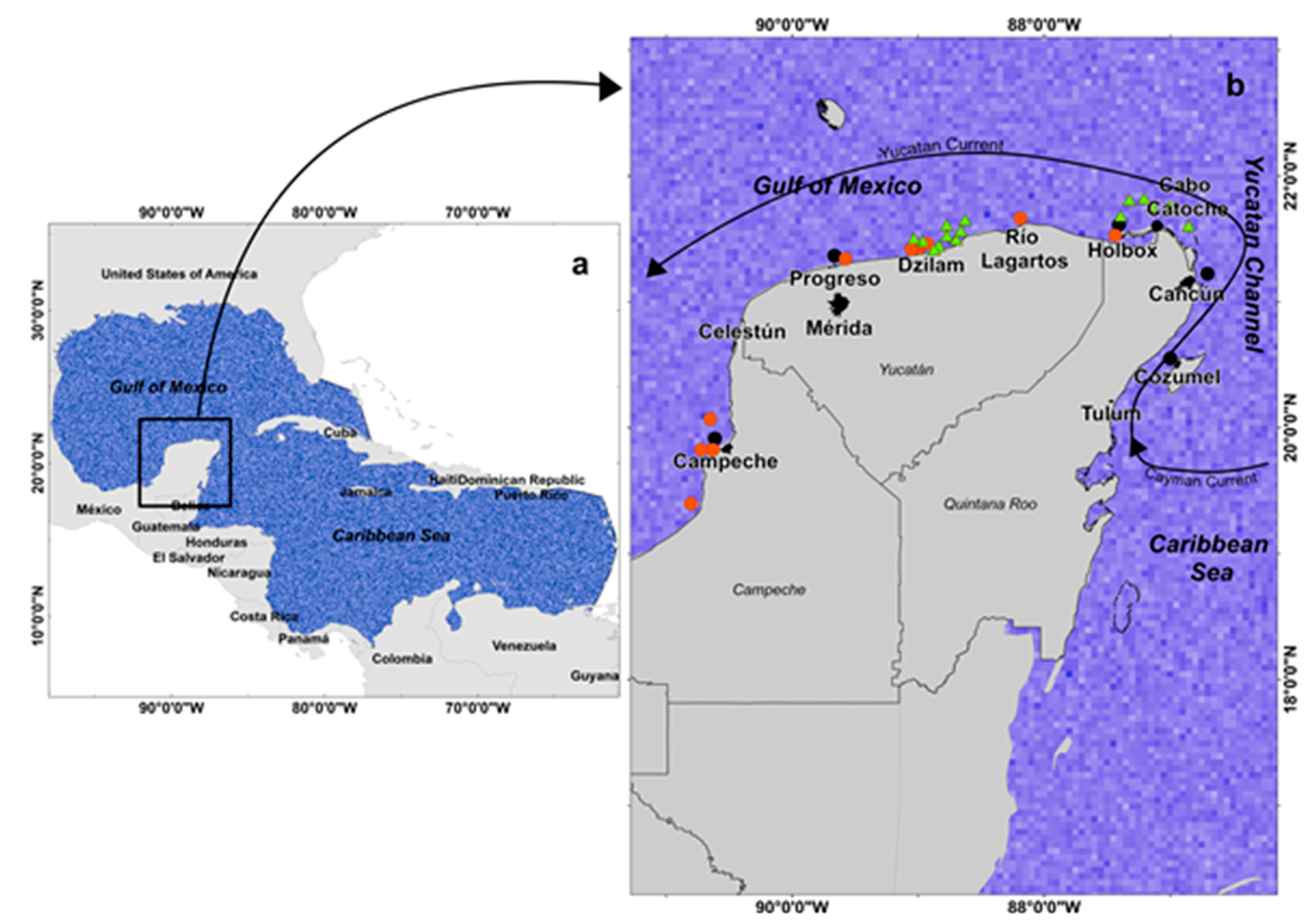
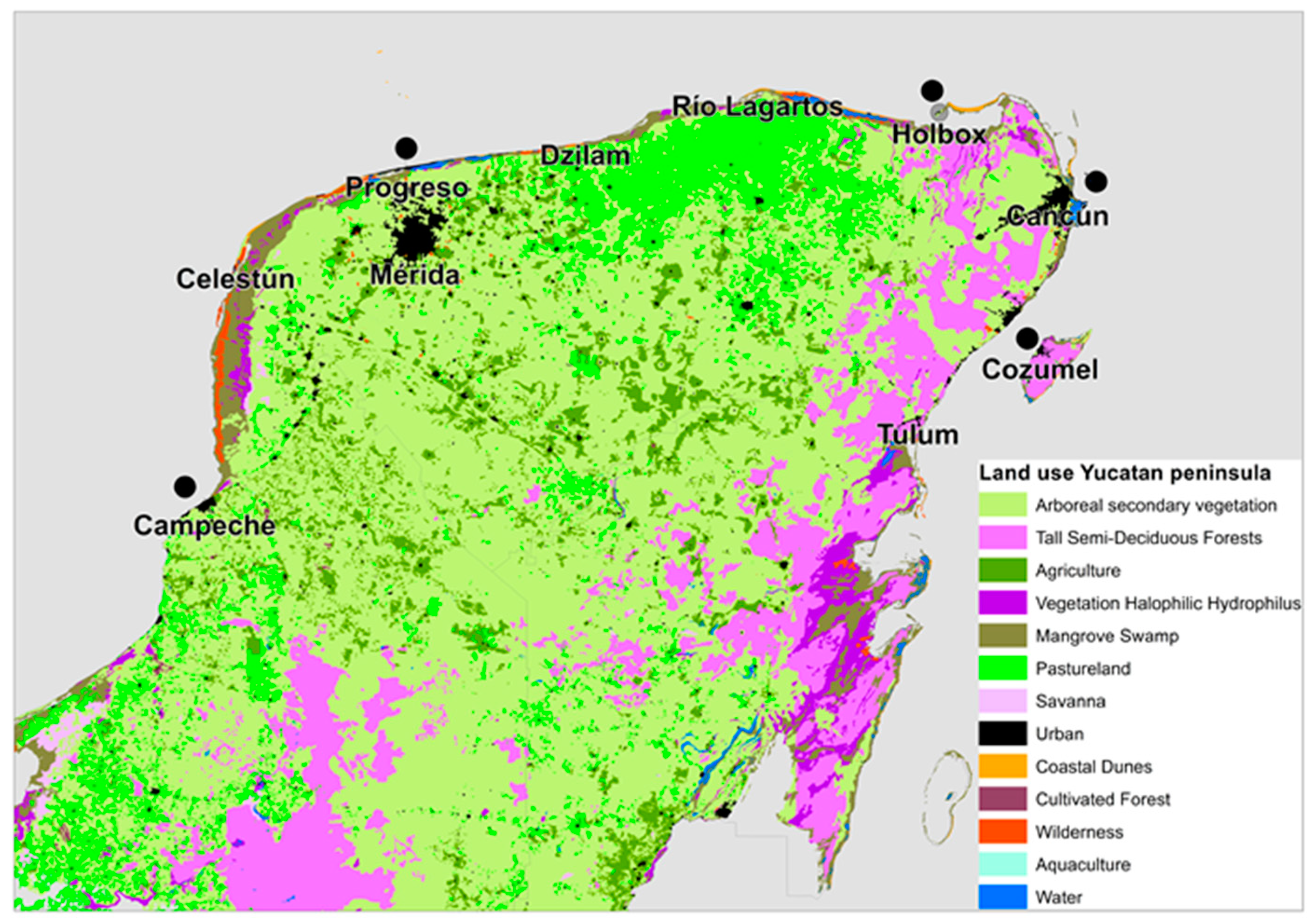
2.1. Case Study Regions

Our study area (Figure 1) comprises the coastal regions of three states of the Yucatán Peninsula: Campeche, Yucatán, and Quintana Roo.

The Yucatán Peninsula separates the Gulf of Mexico Large Marine Ecosystem (GoM-LME) and the Caribbean Sea Large Marine Ecosystem (CS-LME). The Yucatán Current flows into the Gulf of Mexico adjacent to the Yucatán Shelf carrying different water masses from the Caribbean and Atlantic [37] (Figure 1). According to the climatic classification of Koppen modified for Mexico [38], the Yucatán Peninsula has a climatic regime which is predominantly hot and sub-humid, with a dry season from March to May, a rainy season from June to October, and a ‘‘Nortes’’ or post-rainy season from November to February. During the dry season, rainfall is almost absent (1.4 mm) [39,40]. The hydrological unit area of the Yucatán Peninsula Aquifer includes the states of Yucatán, Campeche, and Quintana Roo [41]. It is the most extensive karstic aquifer in the world [42]. It is an unconfined aquifer, except in the coastal zone, characterized by a very low hydraulic gradient on the order of 7–10 mm/km [42]. Nowadays, the aquifer is threatened due to population and tourism infrastructure growth. Among water quality problems, high levels of nutrients and fecal organisms are generalized in both rural and urban areas. The origin of nitrogen and phosphorus concentrations is anthropogenic [43]. López-Maldonado et al. [41] found that 75% of the wastewater from the household sector goes to septic tanks and the remainder is discharged directly into the aquifer, which is in agreement with INEGI (National Institute of Statistic and Geography) [44] statistics. Agriculture and livestock are the other important anthropogenic sources. Particularly, small farms in the livestock sector generate more important direct outputs into the aquifer without treatment than larger farms [41,45]. The connectivity of submarine groundwater discharge to the nearshore coastal environment is an important impact for coastal water quality [46,47,48].

In Figure 2, land uses in the Yucatán Peninsula are represented, and adapted from INEGI 2014 land use cartography (scale 1:250,000). In general terms, the three states show different land uses. In Quintana Roo State, the major land use in the coastal areas are tall semi-deciduous forests, in Yucatan State, the main use is farmland, and in Campeche State, the extent of the mangrove swamp is remarkable.

We selected five monitoring points distributed along the coast of the Yucatán Peninsula (black dots in Figure 1 and Figure 2). The selection was based on important tourist destinations, from east to west: Cozumel, Cancún, Holbox, Progreso, and Campeche. Progreso can be considered as Mérida’s beach. We also took into account historic HABs reported between 2003 and 2017 by COFEPRIS (Comisión Federal para la Protección contra Riesgos Sanitarios/Federal Commission for Protection against Health Risks) [15] in this region (red dots in Figure 1). The population in these municipalities has notably increased over the last years (

Table 1. Inhabitants’ evolution in monitored municipalities (source: INEGI) and monitoring point coordinates.

ID	Coordinate X	Coordinate Y	Location	1990	2000	2010
1	−87.000	20.551	Cozumel	33,884	58,673	77,236
2	−86.705	21.224	Cancun	159,723	392,643	628,306
3	−87.408	21.614	Holbox	927	1193	1486
4	−89.663	21.367	Progreso	35,280	43,850	37,369
	−89.630	20.980	Mérida	522,849	658,698	777,615
5	−90.613	19.914	Campeche	148,211	189,817	220,389

).

The Mexican Caribbean Sea is 40 km wide by 865 km long, which gives an approximate area of 34,000 km² that essentially comprises the coast of the state of Quintana Roo, and indirectly and partially the coast of the state of Yucatán. The Riviera Maya, located along the Caribbean Sea in the state of Quintana Roo, is an internationally known tourist destination, with important tourist centers like Cancún, Holbox, Cozumel, and Tulum (Figure 1). During the decade of the nineties, the hotel sector in the region expanded into a residential hotel corridor of more than 130 km that reaches from Cancún to Tulum. It developed as a massive sun and beach tourism model [49]. More recently, some destinations have sought to differentiate what they offer, such as Holbox Island—a small island on the northeastern tip of the Yucatán Peninsula (Figure 1). Holbox is one of the largest whale shark watching industries in the world, thanks to the congregation of this species from May to September in its plankton rich waters [3].

The high tourism season is summer (from June to September), but there is also an important visitors’ affluence in spring due to Easter holidays and to spring-breakers. Spring-breakers from the USA exceeded 40,000 visitors in 2013–2014 [49].

2.2. Image Processing and Satellite IOP Index Calculations

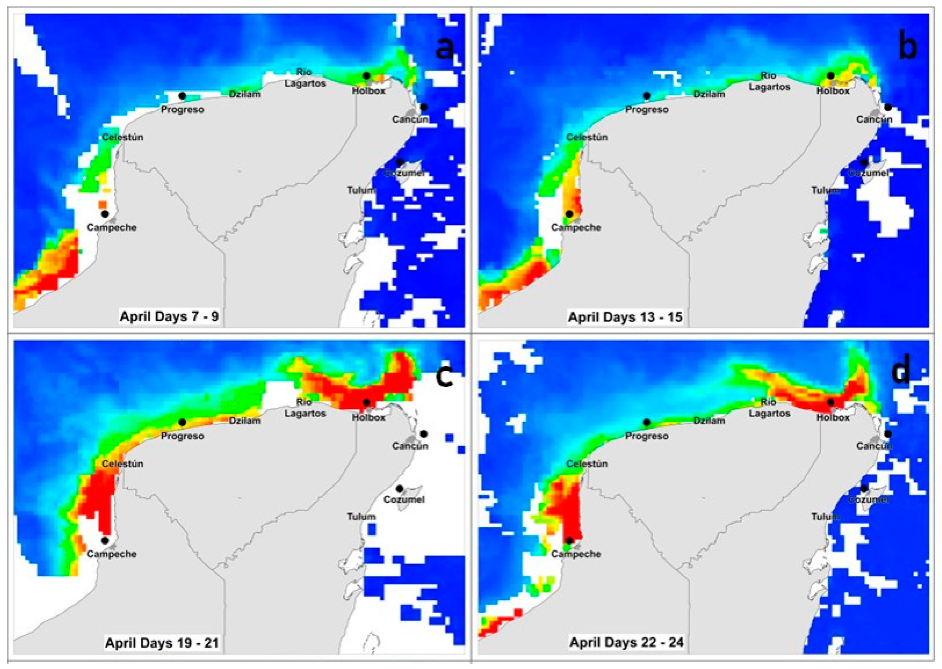
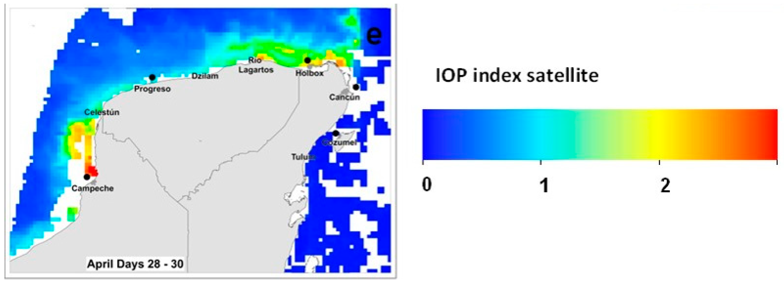
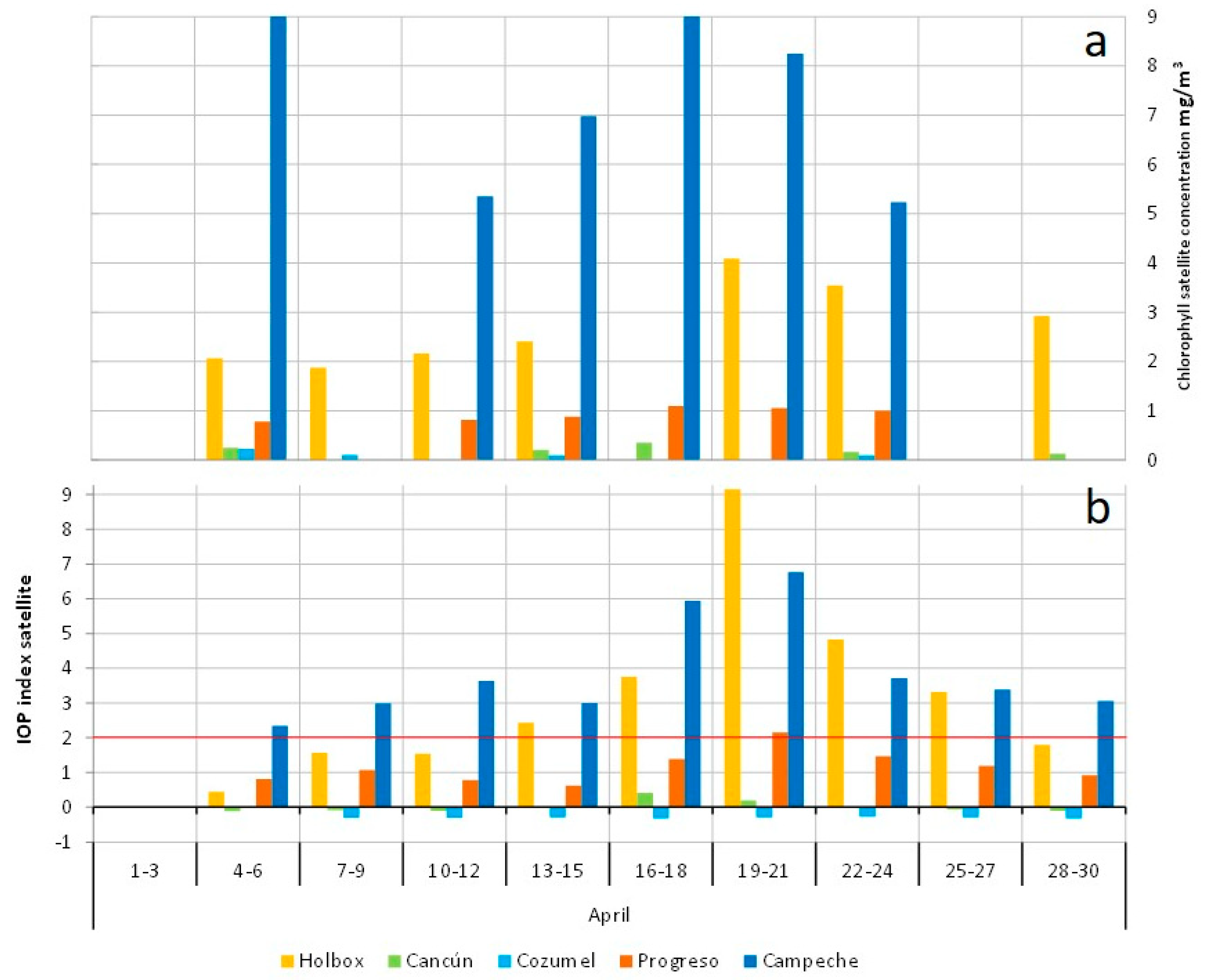
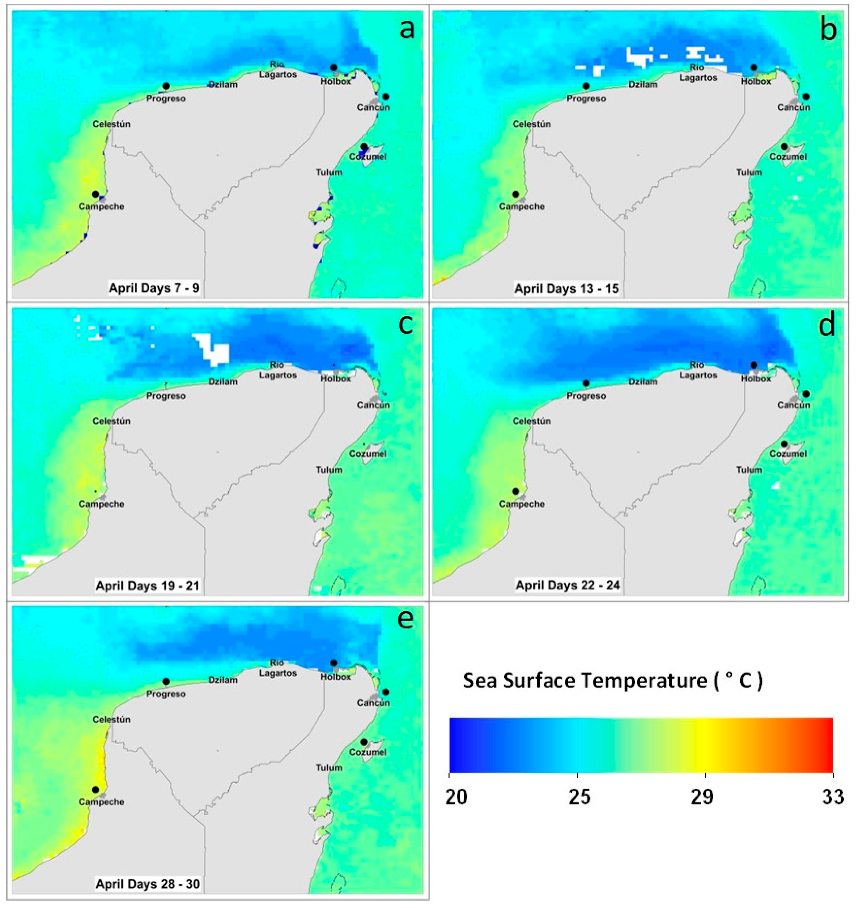
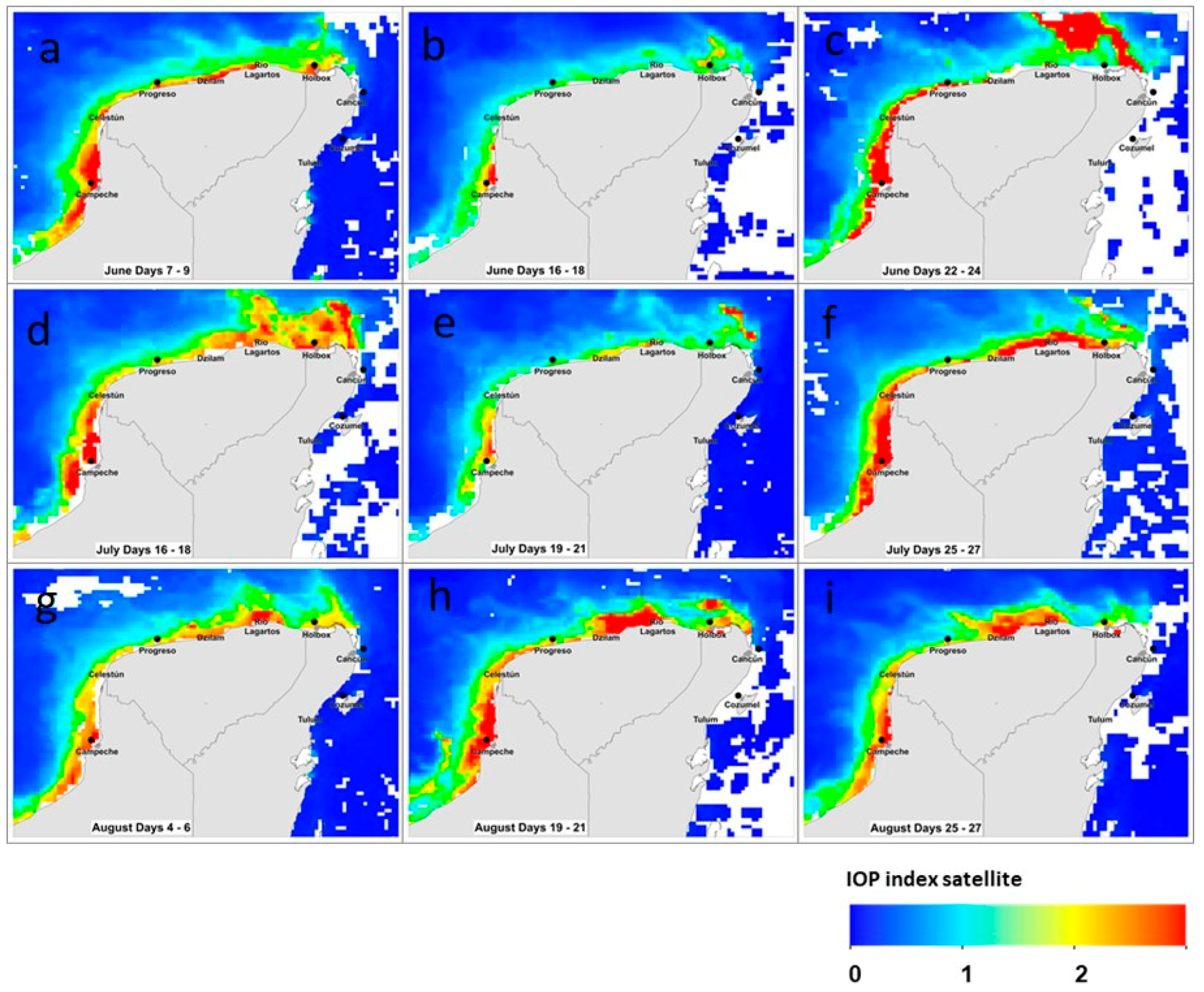
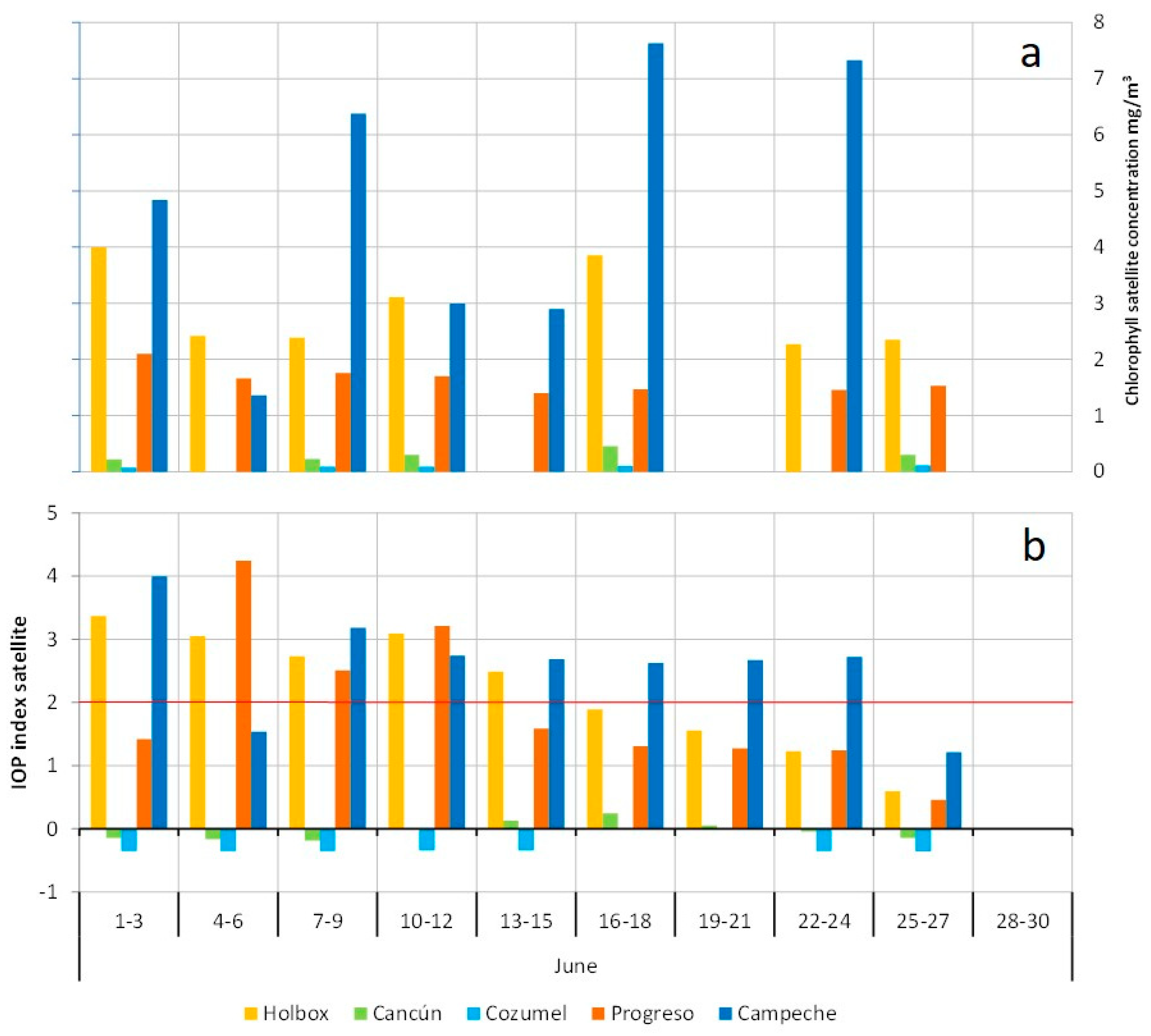
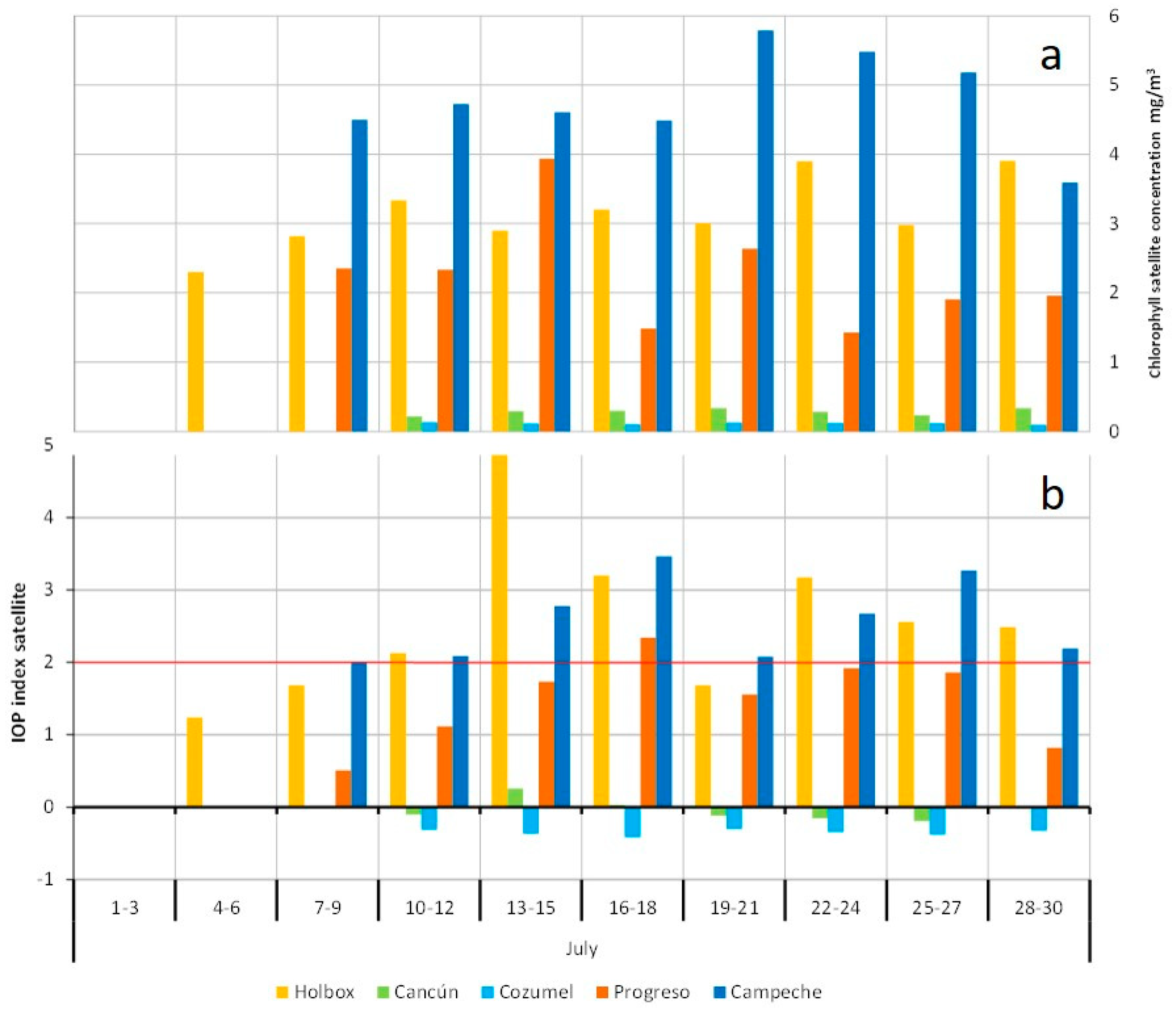
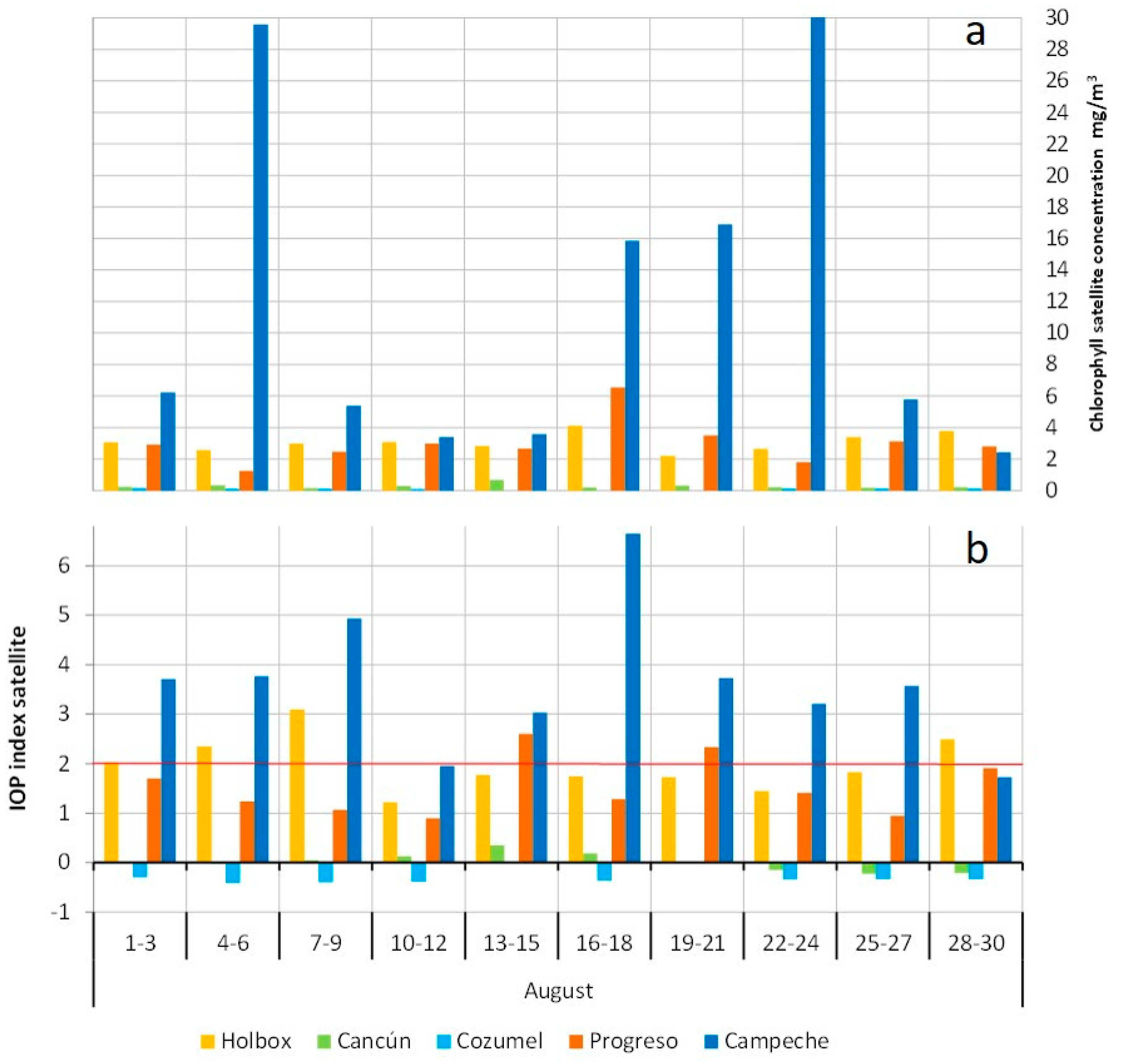
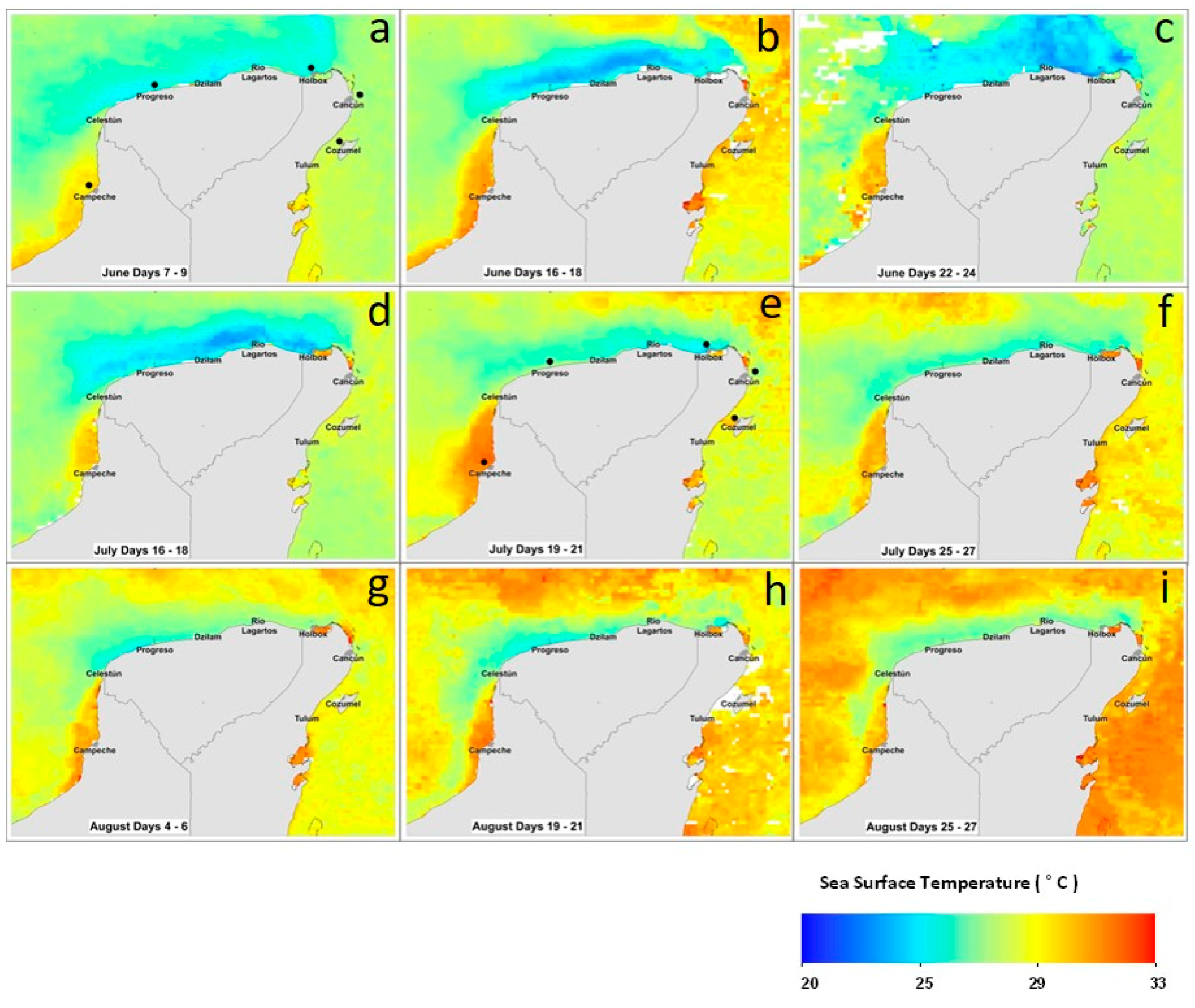
The satellite IOP Index was calculated based on the methodology proposed for the in situ IOP index by Santamaría-del-Ángel et al. [36], and later applied by Aguilar-Maldonado et al. [23] following the next steps. First, the absorption coefficients of phytoplankton and CDM plus CDOM were obtained from the GIOP satellite model. The GIOP model of MODIS Terra and MODIS Aqua sensors were obtained from NASA’s Ocean Color Web. The GIOP model is the result of two international IOP algorithm workshops that were hosted by NASA in conjunction with the Ocean Optics XIX (October 2008) and XX (September 2010) conferences. (Please, see https://oceancolor.gsfc.nasa.gov/atbd/giop/ for more information). We used daily images, processed at level 3, and with 4 km spatial resolution, to form three-day aggregates. Cloud cover prevented us from using daily images. We used the NASA SeaDAS software (https://seadas.gsfc.nasa.gov/) to make composites of the minimum number of days which had good coverage, which in this case was 3 days. The band 443 was selected because satellite products for absorption coefficients were obtained from this one. The GIOP model was obtained from the satellite reflectances [50], which are first converted to their subsurface values [51]. Each component can be expressed as the product of its concentration-specific absorption coefficient (eigenvector; $a^{*}$) and its concentration or amplitude (eigenvalue; A) [33]:

$$a\left(\lambda \right)=a_w+{\displaystyle \sum }_{i=1}^{N_{\varphi }}{A}_{{\varphi }_i}{a}_{{\varphi }_i}^{*}\left(\lambda \right)+{\displaystyle \sum }_{i=1}^{N_d}{A}_{d_i}{a}_{d_i}^{*}\left(\lambda \right)+{\displaystyle \sum }_{i=1}^{N_g}{A}_{CDO{M}_i}{a}_{CDO{M}_i}^{*}\left(\lambda \right)$$

(1)

where the subscripts indicate contributions by water (w), phytoplankton (Ф), CDM (d), and CDOM. Both $a_{d_i}^{*}\left(\lambda \right)$ and $a_{CDO{M}_i}^{*}\left(\lambda \right)$ are commonly expressed as

$$a_{d,CDOM}^{*}\left(\lambda \right)=\exp \left(-S_{d,CDOM}\lambda \right)$$

(2)

where $S$ determines the spectral dependence $a_{CDOM}$ and is found to be approximately 0.014 nm⁻¹ [51]. S_d and S_CDOM typically vary between 0.01 and 0.02 nm⁻¹ in natural waters [52]. As the spectral shapes of CDM and CDOM absorption differ only in their exponential slopes, the two components are typically combined for satellite applications [33].

Then, absorption coefficients of phytoplankton, and CDM plus CDOM were standardized for the wavelength of 443 nm using the equation:

$$z=\frac{x-\overline{x}}{SD}$$

(3)

where: ($x$): the value to be standardized; ($\overline{x}$): the average; and (SD): the standard deviation.

The standardization was calculated for the entire GoM and CS area (Figure 1a) in order to better define baseline conditions and normal patterns.

Then, the satellite IOP Index was calculated based on a principal component analysis (PCA) of the standardized pixel values of each three-day composite. The first principal component was selected because it accounts for the largest possible variance. This selection was based on the eigenvalues. The coefficients of this principal component were named as $b_{\mathbf{1},\mathbf{1}}$ and $b_{\mathbf{1},\mathbf{2}}$. Finally, the IOP Index was calculated based on this first standardized empirical orthogonal function (SEOF1) according to Equation (3).

$$IO{P}_{indexsatellite}=\left[(b_{\mathbf{1},\mathbf{1}}*Z{a}_{\varphi {,}_{GIOP}})+(b_{\mathbf{1},\mathbf{2}}*Z{a}_{dCDOM{,}_{GIOP}})\right]$$

(4)

where $Z{a}_{\varphi {,}_{GIOP}}$ and $Z{a}_{dCDOM{,}_{GIOP}}$ are the standardized values of phytoplankton and CDM (non-algal particles) plus CDOM, respectively, obtained from the GIOP satellite model.

Chlorophyll a concentration and temperature daily images were downloaded and processed equally to absorption coefficients.

Images of the dry period (i.e., April) and the wet period (i.e., June, July, and August) of the year 2011 were used. The year 2011 was chosen based on the report of a very extensive bloom in time (it lasted about 150 days from August to December 2011) and space in this region already analyzed from other points of view by other authors [7,23].

To describe the stages of a phytoplankton bloom, the values of the IOP Index were interpreted as follows [23,31]: (1) values in the interval (−1, 1) show the normal values of the specific site or non-bloom conditions; (2) values in the interval (1, 2) are above the average and represent a transition from anomalous values to normal values or decaying bloom conditions; and (3) values higher than 2 are anomalous and indicate eutrophic or bloom conditions. These thresholds are defined thanks to the standardization of the data. In a normal distribution, the Inverse Cumulative Distribution Function (ICDF) defines 1.96 standard deviations as the limit of values without noise with 95% confidence. This value was rounded to 2 standard deviations to define the limit of the anomalous conditions.

A Spearman correlation analysis was performed between GIOP model absorption coefficients and in situ measures of absorption coefficients published in Aguilar-Maldonado et al. [23]. In situ sampling points are represented in Figure 1b. These points are located in Dzilam (Yucatán) and Holbox (Quintana Roo). Nine samples were collected on 27 August and six samples on 30 August 2011. Colored detritus matter and CDOM were added to be compared with the satellite product $a_{dCDOM{,}_{GIOP}}$. Each sampled point was related to the pixel value corresponding to that point.

3. Results

Spearman correlation analysis showed high positive and significant correlation between in situ absorption coefficients and satellite products. Colored detritus matter plus CDOM obtained from the GIOP model has a 0.533 relation with CDM plus CDOM obtained from in situ measures, while phytoplankton coefficients have a 0.937 relation.

In Figure 3, we can see the satellite IOP index results for April 2011. Inherent Optical Properties Index values above two indicate active bloom conditions and they are represented by a yellow to red color scale. Red areas show the highest anomalies. White areas are not covered by satellite due to clouds. April 2011 was the driest month according to SMN (National Meteorological Service) [53] with a 21.9 mm average precipitation. In 2011, spring break was from 15 March to 15 April and approximately 30,000 visitors were registered [48]. The first April fortnight, we observe bloom conditions in the coastal area of Campeche State (Figure 3a,b, red areas), and with less intensity around Holbox Island (Figure 3a,b yellow areas). During the second fortnight, bloom conditions expand on the North Campeche coast (Figure 3c,d, red areas), and extend from Holbox to Río Lagarto (Figure 3c,d red areas). During the last April days, from the 28 to 30, the phytoplankton blooms were considerably reduced (Figure 3e, yellow and orange areas). During this period, no phytoplankton bloom was detected in the southern coastal region of Quintana Roo State. In Figure 4, we represent the satellite IOP Index values for the five selected monitoring points: Holbox, Cancún, Cozumel, Progreso, and Campeche. These points are represented as black dots on Figure 1 and Figure 2, and their coordinates are included in Table 1. Figure 4 is supplementary to Figure 3, and includes the whole April period for the monitoring points. As we can see, satellite coverage in the Cancún area was less than for the rest of the Yucatán Peninsula; white areas in Figure 3 are those without satellite images due to cloud cover, and in Figure 4 correspond to no data. However, the Cozumel monitoring point, which is the closest point to Cancún in Quintana Roo State, had a better coverage and satellite IOP Index, which was always between (−1, 0), which indicates non-bloom conditions. The Progreso monitoring point showed values in the interval (1, 2) which were above the average and represented decaying bloom conditions. Only during 19 to 21 April did the IOP Index exceeds 2 (2.16), indicating an active bloom. On the other hand, Campeche and Holbox showed the highest values. The IOP Index was above two during the entire month at the Campeche monitoring point, with maximum values from 16 to 21 April (IOP index from 5.94 to 6.77). The Holbox monitoring point was above two from 13 to 27 April, with a maximum value of 9.16 from 19 to 21 April.

Figure 4 shows the relationship of the satellite IOP index with satellite chlorophyll a. We observe that anomalous values of the index (>2), which mean active bloom conditions are characterized by the highest chlorophyll a concentrations. In Campeche region, all points with an IOP index value above two had chlorophyll a concentrations between 5 to 9 mg/m³. In Holbox, points classified as in active bloom had chlorophyll a concentrations between 2 to 4 mg/m³. Due to clouds not all monitoring points had chlorophyll a data for the whole study period, this is reflected in the absence of bars in Figure 4 for those data.

Figure 5 illustrates sea surface temperature in the coastal waters of the Yucatán Peninsula during the dry period. A cooler water mass can be observed in the northern region approximately from Progreso to Holbox, while in the east a warmer water mass predominated. It can be seen that the satellite IOP Index is related to the movement of water masses. In general, cooler waters from the Gulf of Mexico are associated with anomalous values.

In Figure 6, we represent a selection for the wet period (i.e., June–August 2011) which coincides with summer and the highest visitor number period. June was the rainiest month according to SMN (National Meteorological Service) [53], with a 234.3 mm average precipitation. During this period, the entire coastal area of the Yucatán and Campeche states, and the Holbox area (Quintana Roo), show satellite IOP Index values higher than two, depicted by a yellow to red color scale (Figure 6). As in April, no phytoplankton bloom was detected in the southern coastal region of Quintana Roo State, which includes the Cozumel and Cancún municipalities (Figure 6).

Figure 7, Figure 8 and Figure 9 are supplementary to Figure 6, and include the whole June to August period for the selected monitoring points. During the wet period, Cancún and Cozumel remained in the interval (−1, 1) which represents the average value for the CS-LME, and represents non-bloom conditions. At the Progreso monitoring point, which was in the interval (1, 2) in June, showed IOP index values above two from 4 to 12 June (Figure 7), and punctually between 16 to 18 July (Figure 8), and from 13 to 15 August (Figure 9). Holbox was in bloom conditions mainly during the first June fortnight (Figure 7) and the second July fortnight (Figure 8), but also for some days in August (Figure 9, 4 to 9 August and 28 to 30 August). Campeche was in active bloom conditions (IOP Index > 2) during nearly the entire wet period (Figure 7, Figure 8 and Figure 9), and only sporadically showed values in the interval (1, 2) which represent decaying bloom conditions (e.g., Figure 7, 4 to 6 June).

In these same figures, chlorophyll a concentrations are shown. The anomalous values of the IOP Index are associated with the highest chlorophyll a concentrations. In the Campeche region, all points with an IOP Index value above two had chlorophyll a concentrations approximately between 3 to 30 mg/m³. The highest chlorophyll a concentrations were detected in August. Higher concentrations of chlorophyll a than in the dry period were observed. In Holbox, points classified as in active bloom had chlorophyll a concentrations between 2 to 4 mg/m³.

The satellite IOP Index is based on the three optically important components of water, not just phytoplankton. Sometimes, high values of chlorophyll a are linked to low IOP Index values close to the threshold between active bloom and decaying bloom conditions. This is because the concentration of CDOM is very high due to the degradation of organic matter, that is, the degradation of the dead phytoplankton that formed the bloom. Therefore, although the concentration of chlorophyll a remains high, it is considered that the bloom is in decay when the value of the IOP is less than two. A downward trend in the value of the IOP indicates an increase in the processes of degradation of organic matter or external contributions of CDM.

Figure 10 illustrates sea Surface Temperature in the coastal waters of the Yucatán Peninsula during the wet period (June to August), and a significant surface water warming was observed.

4. Discussion

As stated by Carstensen et al. [54], “while there is no universally accepted definition of what constitutes a bloom, the notion of a substantial deviation above background phytoplankton biomass is common to all definitions”. So, we can define a phytoplankton bloom as a deviation to higher values than standard seasonal patterns at a specific site. Unusual high phytoplankton biomass values can be very different between sites. For instance, Carstensen et al. [54] studied long-term monitoring data from a diverse set of marine ecosystems in North America and Northwestern Europe and observed an important difference in biomass scale between sites. The Yucatan Basin has been described as an oligotrophic region devoid of nutrients in the surface layer [16]. In the absence of phytoplankton blooms, chlorophyll a levels observed in this area by other studies did not exceed 1.65 mg m⁻³ [17]. Chlorophyll a levels above 2 mg m⁻³ have been classified as a eutrophic regime by several authors [18,19,20]. In this study, we found that chlorophyll a values above 2 mg m⁻³ in the Holbox area have been classified as in bloom conditions according to the IOP Index. This may seem a reduced chlorophyll a value, but it is not for this specific area, since it represents a substantial deviation from background values.

Biomass patterns in estuarine-coastal ecosystems can change abruptly [55]. In general, it is a recognized one seasonal pattern that starts with a spring bloom dominated by large, fast-growing diatoms, followed by a number of summer blooms comprised of diatoms, flagellates, and dinoflagellates. However, there are many deviations from this classical pattern [54]. The high variability of coastal waters promotes different strategies at different times and a unique pattern of bloom occurrence cannot be defined [56,57]. The presence of a quasi-permanent bloom in the Campeche region could be explained because of the succession of different species, and sustained due to all the processes that have been identified to trigger blooms at the land-sea interface, including coastal upwelling, wind induced entrainment of bottom water, neap-spring variability of tidal mixing and stratification, seasonal winds that enhance water retention in bays, and seasonal changes in temperature and solar radiation, among others [54]. The temporal and spatial distribution of phytoplankton blooms shown in the results section is the consequence of several factors, including both oceanographic and continental processes. Among them, upwelling events, oceanographic currents, and submarine groundwater discharges (SGDs). The northeastern coast of Yucatan is nourished by seasonal coastal upwelling events which have positive effects such as enhancing fisheries and promoting the presence of the whale shark, but also undesired effects like algal bloom events [37]. It is known to upwell during spring and summer. While upwelling could be suppressed during the northerly winds season (90–129 m/s), these winds contribute to the cooling and mixing of the water column from October to April [21,37]. In our study, we selected April, June, July, and August as the study period taking into account not only tourist activity but also these upwelling events. The surface circulation in the central portion of the Gulf is dominated by the Loop Current, where surface waters enter into the Gulf through the Yucatán channel and exit through the Florida Strait [21,58]. North of Cabo Catoche (Figure 1), a cyclonic gyre formation marks the area of most intensive upwelling in the Yucatan region. According to Pérez et al. [59], this gyre, in addition, may define a focus of convergence of upwelled and Yucatan Current waters. Another feature described by Pérez et al. [59] is a permanent countercurrent, which flows to the southwest along the slope of the Yucatan Peninsula which may be related to the upwelling-convergence processes. In Figure 5 and Figure 10, we observed that the nearest coastal stripe was characterized by more constant sea surface temperatures, and it is well marked both during the dry and wet periods. These authors [59] found high concentrations of chlorophyll, organic particles, and phytoplankton around the northeast of Cabo Catoche in the summer. These high concentrations match our results in Figure 6, where we observe high IOP Index values, due to phytoplankton blooms, in the Río Lagartos-Holbox area. In the Campeche area, inside the Gulf of Mexico, the Campeche bank has been described as one of the most important upwelling regions in the western ocean margin [60]. Both in Figure 4 and Figure 6, we can observe characteristic high IOP Index values.

Submarine groundwater discharges in the Yucatán karstic aquifer, where the aquifer is connected hydraulically with the sea, provides a direct input of nutrients such as nitrogen (N) and phosphorus (P) to coastal waters. Several authors have found evidence that water quality is strongly related to SGD, and variations in phytoplankton community structure are related to local nutrient loading and hydrographic conditions, turbulence, and human impacts [47,48]. This nutrient input is usually characterized by N:P ratios higher than 16, which is the optimal ratio for algae in coastal areas (Redfield ratio), especially in agricultural areas [61]. Groundwater quality is also influenced by the amount and distribution of precipitation [62]. Muñoz et al. [63] found higher levels of phosphate during the wet season in the Dzilam area, which is characterized by livestock uses (Figure 2). Pacheco et al. [62] found high nitrate concentrations under the biggest city in Yucatan State (Mérida) and in the agricultural zone, which cause an increase in this ratio. But, phosphorus inputs from domestic and municipal sewage can also modify the Redfield ratio. While nitrate inputs are usually linked to agriculture, phosphorus inputs can be linked to tourism, as their main source is domestic sewage [64]. However, this karst system is characterized by delayed groundwater discharge [42], and a lag may exist before peak discharge of groundwater and nutrients to the coast occurs [46]. In our results, we observed important phytoplankton blooms in the Holbox-Río Lagarto area since 19 to 24 April. This year, 2011, the spring break was from 15 March to 15 April. So, blooms in this area started approximately one month after the beginning of the maximum hotel occupation. Upwelling events also happened during spring, but it seems that the added effect of SGDs could have triggered phytoplankton blooms.

In our results we observed that phytoplankton blooms extended from Holbox (most eastern area with bloom events) to South Campeche, while no blooms were observed in the Cancún-Cozumel area. Historic COFEPRIS reports of HABs from 2003 to 2017 [10], which are represented with red dots in Figure 1, show the same spatial distribution. This can be due to the effect of the Yucatan Current, which flows into the Gulf of Mexico adjacent to the Yucatan Shelf carrying different water masses from the Caribbean and Atlantic (Figure 1 arrow indicates the Yucatán current direction). Enriquez et al. [65] already noticed that a bloom seeded in the Cabo Catoche (CC) region will move along the coast travelling westwards. During the dry period, no blooms were reported by COFEPRIS [15], although we found blooming areas in Campeche and Holbox. During the 2011 wet period, COFEPRIS [15] did report blooms. COFEPRIS [15] reported a HAB of Scrippsiella trochoidea, Pleurosigma sp., and Cylindrotheca closterium between 22 July to 16 December on Río Lagartos (Yucatán state), but no sanitary closure was implemented. However, we observed satellite IOP Index values above two from 1 June in the Holbox-Río Lagartos area, which indicated an active phytoplankton bloom. The next HAB reported by COFEPRIS was on 15 October and lasted until 18 October on Holbox (Quintana Roo state). This HAB did imply the sanitary closure and the death of 4 tons of fish was quantified [15]. So, no HAB was detected in Holbox until October, but we have shown that active bloom conditions were present along the June–August period, and also after the spring break. These active bloom conditions were characterized by a high phytoplankton biomass, as corroborated by satellite chlorophyll a graphs included in the results section (Figure 4 and Figure 7–9). Also, the studies of References [7,23] confirm high phytoplankton biomass blooms. The Permanent Monitoring Program of Harmful Algal Blooms [10] is based not on regular monitoring but on direct observation and reporting to the authorities. The major consequence of this type of monitoring is that HAB events can go unnoticed. In addition, water color in optically complex waters depends on its three main constituents: CDM, CDOM, and chlorophyll a [34,35]. So, observing water color is not a confident way to detect blooms because it can confuse it with high CDM or high CDOM content. The advantage of the IOP Index is that it can discern phytoplankton biomass blooms from discoloration due to CDM or CDOM as proven by Reference [23]. The IOP Index cannot give information on phytoplankton taxonomic composition, so by its results we are not able to detect the presence of toxic species. But it has proven very useful to map blooming areas, which is essential to plan in situ sampling and optimize sampling efforts. Not all HABs produce fish mortalities as can be appreciated in COFEPRIS reports, but they have other undesired effects such as reduced water transparency. Ziegler et al. [3] identified the most important motivations for participating in the whale shark tour on Holbox as good underwater visibility and proximity to whale sharks. However, a significant proportion of tour participants were dissatisfied with underwater visibility (22.9%), the variety of marine life (20.2%), and abundance of marine life (19.5%). All these environmental features can be seriously affected by phytoplankton bloom events. Understanding tourist needs and expectations can help inform management decisions and improve the quality of services offered at a particular tourism destination.

Continuous monitoring is of paramount importance for implementing preventive and corrective measures. The use of satellite products can enhance in situ monitoring possibilities, as it offers higher spatial and temporal resolution at a lower cost [23,24,25,26]. However, these products must be used with caution. Our methodology offers a more precise technology because the satellite IOP Index has taken into account all the water constituents (i.e., phytoplankton, CDOM, and CDM) to identify an active bloom [23,36]. Other products such as the diffuse attenuation coefficient K490 (m⁻¹) is not able to distinguish active bloom conditions, because high KD490 values can be due to other water constituents rather than to chlorophyll a [7]. The application of the satellite IOP Index can help to build baseline information in a sustainable mid-term or long-term basis which is key for ecosystem-based management. Following the approach of Stankey et al. [6], we could use the satellite IOP Index as an indicator to determine the Limits of Acceptable Change (LAC). The first step in the process of establishing LAC is identifying desirable ecological conditions and choosing indicators of these conditions. Ecological desired conditions are IOP Index values below two, which indicate an absence of an active phytoplankton bloom. The second step is assessing current conditions, which will imply determining the location, extension, and frequency of active blooms. Long-term monitoring data is necessary to define the standard seasonal pattern of a specific site. The following steps are identifying management actions, and monitoring and evaluating those implemented management actions. The advantage of remote sensing is that due to its reduced cost, it is more feasible for implementing an economically sustainable monitoring program. Tourism satisfaction with water quality and transparency could be related to the presence of active or decaying bloom conditions which produce reduced water clarity. Natural processes, such as the Yucatán Current, avoid that the impact of tourist industry can be seen in the main tourism centers (e.g., Cancún to Tulum, in the Riviera Maya). But, this does not mean that wastewater discharges to septic tanks have no effect, it rather means that their effect is observed in areas further away (e.g., Holbox). In this framework, management actions, cannot be local actions, but must move a step forward to take into account regional processes. In this sense, remote sensing can be a useful tool in monitoring programs.

References

1. Bentz, J.; Lopes, F.; Calado, H.; Dearden, P. Sustaining marine wildlife tourism through linking Limits of Acceptable Change and zoning in the Wildlife Tourism Model. Mar. Policy 2016, 68, 100–107. [Google Scholar] [CrossRef]
2. Jarvis, D.; Stoeckl, N.; Liu, H. The impact of economic, social and environmental factors on trip satisfaction and the likelihood of visitors returning. Tour. Manag. 2016, 52, 1–18. [Google Scholar] [CrossRef]
3. Ziegler, J.; Dearden, P.; Rollins, R. But are tourists satisfied? Importance-performance analysis of the whale shark tourism industry on Isla Holbox, Mexico. Tour. Manag. 2012, 33, 692–701. [Google Scholar] [CrossRef]
4. Padilla, N.S. The environmental effects of Tourism in Cancun, Mexico. Int. J. Environ. Sci. 2015, 6, 282–294. [Google Scholar] [CrossRef]
5. Duffus, D.A.; Dearden, P. Non-consumptive wildlife-oriented recreation, a conceptual framework. Biol. Conserv. 1990, 53, 213–231. [Google Scholar] [CrossRef]
6. Stankey, G.H.; McCool, S.F.; Stokes, G.L. Limits of acceptable change: A new framework for managing the Bob Marshall wilderness complex. West. Wildlands 1984, 10, 33–37. [Google Scholar]
7. Aguilar-Trujillo, A.C.; Okolodkov, Y.B.; Herrera-Silveira, J.A.; Merino-Virgilio, F.D.C.; Galicia-García, C. Taxocoenosis of epibenthic dinoflagellates in the coastal waters of the northern Yucatan Peninsula before and after the harmful algal bloom event in 2011–2012. Mar. Pollut. Bull. 2017, 119, 396–406. [Google Scholar] [CrossRef] [PubMed]
8. Ulloa, M.J.; Álvarez-Torres, P.; Horak-Romo, K.P.; Ortega-Izaguirre, R. Harmful algal blooms and eutrophication along the Mexican coast of the Gulf of Mexico large marine ecosystem. Environ. Dev. 2017, 22, 120–128. [Google Scholar] [CrossRef]
9. Henrichs, D.W.; Hetland, R.D.; Campbell, L. Identifying bloom origins of the toxic dinoflagellate Karenia brevis in the western Gulf of Mexico using a spatially explicit individual-based model. Ecol. Model. 2015, 313, 251–258. [Google Scholar] [CrossRef]
10. Murray, G. Constructing Paradise: The Impacts of Big Tourism in the Mexican Coastal Zone. Coast. Manag. 2007, 35, 339–355. [Google Scholar] [CrossRef]
11. Castillo-Pavón, O.; Méndez-Ramírez, J.J. The tourist developments and their environmental effects in the Mayan Riviera, 1980–2015. Quivera 2017, 19, 101–118. [Google Scholar]
12. Heisler, J.; Glibert, P.M.; Burkholder, J.M.; Anderson, D.M.; Cochlan, W.; Dennison, W.C.; Dortch, Q.; Gobler, C.J.; Heil, C.A.; Humphries, E.; et al. Eutrophication and harmful algal blooms: A scientific consensus. Harmful Algae 2008, 8, 3–13. [Google Scholar] [CrossRef] [PubMed] [Green Version]
13. Smayda, T.J. Complexity in the eutrophication–harmful algal bloom relationship, with comment on the importance of grazing. Harmful Algae 2008, 8, 140–151. [Google Scholar] [CrossRef]
14. Klemas, V. Remote sensing of algal blooms: An overview with case studies. J. Coast. Res. 2012, 28, 34–43. [Google Scholar] [CrossRef]
15. COFEPRIS (Comisión Federal para la Protección contra Riesgos Sanitarios/Federal Commission for Protection against Health Risks). Available online: https://www.gob.mx/cofepris/acciones-y-programas/antecedentes-en-mexico-76707 (accessed on 9 March 2018).
16. Okolodkov, Y.B. A review of Russian plankton research in the Gulf of Mexico and the Caribbean Sea in the 1960–1980s. Hidrobiológica 2003, 13, 207–221. [Google Scholar]
17. Signoret, M.; Bulit, C.; Pérez, R. Patrones de distribución de clorofila ay producción primaria en aguas del Golfo de México y del Mar Caribe. Hidrobiológica 1998, 8, 81–88. [Google Scholar]
18. Antoine, D.; Morel, A. Oceanic primary production: 1. Adaptation of a spectral light-photosynthesis model in view of application to satellite chlorophyll observations. Glob. Biogeochem. Cycles 1996, 10, 43–55. [Google Scholar] [CrossRef]
19. Barocio-León, Ó.A.; Millán-Núñez, R.; Santamaría-del-Ángel, E.; González-Silvera, A.; Trees, C.C. Spatial variability of phytoplankton absorption coefficients and pigments off Baja California during November 2002. J. Oceanogr. 2006, 62, 873–885. [Google Scholar] [CrossRef]
20. Smith, V.H.; Tilman, G.D.; Nekola, J.C. Eutrophication: Impacts of excess nutrient inputs on freshwater, marine, and terrestrial ecosystems. Environ. Pollut. 1999, 100, 179–196. [Google Scholar] [CrossRef]
21. Limoges, A.; Londeix, L.; de Vernal, A. Organic-walled dinoflagellate cyst distribution in the Gulf of Mexico. Mar. Micropaleontol. 2013, 102, 51–68. [Google Scholar] [CrossRef]
22. Jiang, L.; Xia, M.; Ludsin, S.A.; Rutherford, E.S.; Mason, D.M.; Pangle, K.L.; Marin Jarrin, J.R. Biophysical modeling assessment of the drivers for plankton dynamics at western Lake Erie. Ecol. Model. 2015, 308, 18–33. [Google Scholar] [CrossRef]
23. Aguilar-Maldonado, J.A.; Santamaría-del-Ángel, E.; González-Silvera, A.; Cervantes-Rosas, O.; López, L.M.; Gutiérrez-Magness, A.; Cerdeira-Estrada, S.; Sebastiá-Frasquet, M.T. Identification of Phytoplankton Blooms under the Index of Inherent Optical Properties (IOP Index) in Optically Complex Waters. Water 2018, 10, 129. [Google Scholar] [CrossRef]
24. Sebastiá Frasquet, M.T.; Estornell Cremades, J.; Rodilla Alamá, M.; Marti Gavila, J.; Falco Giaccaglia, S.L. Estimation of chlorophyll «A» on the Mediterranean coast using a QuickBird image. Revista de Teledetección 2012, 37, 23–33. [Google Scholar]
25. Caroppo, C.; Odermatt, D.; Philipson, P.; Bruno, M. Using satellite remote sensing of harmful algal blooms (HABs) in a coastal European site. Phycologia 2017, 56, 28. [Google Scholar]
26. Wei, G.; Tang, D.; Wang, S. Distribution of chlorophyll and harmful algal blooms (HABs): A review on space based studies in the coastal environments of Chinese marginal seas. Adv. Space Res. 2008, 41, 12–19. [Google Scholar] [CrossRef]
27. Urquhart, E.A.; Schaeffer, B.A.; Stumpf, R.P.; Loftin, K.A.; Werdell, P.J. A method for examining temporal changes in cyanobacterial harmful algal bloom spatial extent using satellite remote sensing. Harmful Algae 2017, 67, 144–152. [Google Scholar] [CrossRef] [PubMed]
28. Harvey, E.T.; Kratzer, S.; Philipson, P. Satellite-based water quality monitoring for improved spatial and temporal retrieval of chlorophyll-a in coastal waters. Remote Sens. Environ. 2015, 158, 417–430. [Google Scholar] [CrossRef]
29. Malthus, T.J.; Mumby, P.J. Remote sensing of the coastal zone: An overview and priorities for future research. Int. J. Remote Sens. 2003, 24, 2805–2815. [Google Scholar] [CrossRef] [Green Version]
30. Matthews, M.W. A current review of empirical procedures of remote sensing in inland and near-coastal transitional waters. Int. J. Remote Sens. 2011, 32, 6855–6899. [Google Scholar] [CrossRef]
31. Miller, R.L.; McKee, B.A. Using MODIS Terra 250 m imagery to map concentrations of total suspended matter in coastal waters. Remote Sens. Environ. 2004, 93, 259–266. [Google Scholar] [CrossRef] [Green Version]
32. Loisel, H.; Vantrepotte, V.; Norkvist, K.; Mériaux, X.; Kheireddine, M.; Ras, J.; Pujo-Pay, M.; Combet, Y.; Leblanc, K.; Dall’Olmo, G.; et al. Characterization of the Bio-Optical Anomaly and Diurnal Variability of Particulate Matter, as Seen from Scattering and Backscattering Coefficients, in Ultra-Oligotrophic Eddies of the Mediterranean Sea. Biogeosciences 2011, 8, 3295–3317. [Google Scholar] [CrossRef]
33. Werdell, P.J.; Franz, B.A.; Bailey, S.W.; Feldman, G.C.; Boss, E.; Brando, V.E.; Dowell, M.; Hirata, T.; Lavender, S.J.; Lee, Z.; et al. Generalized ocean color inversion model for retrieving marine inherent optical properties. Appl. Opt. 2013, 52, 2019–2037. [Google Scholar] [CrossRef] [PubMed] [Green Version]
34. Brezonik, P.L.; Olmanson, L.G.; Finlay, J.C.; Bauer, M.E. Factors affecting the measurement of CDOM by remote sensing of optically complex inland waters. Remote Sens. Environ. 2015, 157, 199–215. [Google Scholar] [CrossRef]
35. Odermatt, D.; Gitelson, A.; Brando, V.E.; Schaepman, M. Review of constituent retrieval in optically deep and complex waters from satellite imagery. Remote Sens. Environ. 2012, 118, 116–126. [Google Scholar] [CrossRef] [Green Version]
36. Santamaría-del-Angel, E.; Soto, I.; Millán-Nuñez, R.; González-Silvera, A.; Wolny, J.; Cerdeira-Estrada, S.; Cajal-Medrano, R.; Muller-Karger, F.; Cannizzaro, J.; Padilla-Rosas, Y.; et al. Experiences and Recommendations for Environmental Monitoring Programs. In Environmental Science, Engineering and Technology; Sebastia-Frasquet, M.-T., Ed.; Nova Science Publishers: Hauppauge, NY, USA, 2015; p. 32. ISBN 978-1-63482-189-6. [Google Scholar]
37. Enriquez, C.; Mariño-Tapia, I.; Jeronimo, G.; Capurro-Filograsso, L. Thermohaline processes in a tropical coastal zone. Cont. Shelf Res. 2013, 69, 101–109. [Google Scholar] [CrossRef]
38. García, E. Modificaciones al Sistema Climático de Köppen para la República Mexicana, 5th ed.; Instituto de Geografía: Ciudad de Mexico, Mexico, 2004; ISBN 970-32-1010-4. [Google Scholar]
39. CONAGUA (Comisión Nacional del Agua/National Water Comission). Estadísticas del Agua en México. Secretaría de Medio Ambiente y Recursos Naturales. 2016. Available online: http://201.116.60.25/publicaciones/EAM_2016.pdf (accessed on 2 February 2018).
40. Arcega-Cabrera, F.; Garza-Pérez, R.; Noreña-Barroso, E.; Oceguera-Vargas, I. Impacts of geochemical and environmental factors on seasonal variation of heavy metals in a coastal lagoon Yucatan, Mexico. Bull. Environ. Contam. Toxicol. 2015, 94, 58–65. [Google Scholar] [CrossRef] [PubMed]
41. Lopez-Maldonado, Y.; Batllori-Sampedro, E.; Binder, C.R.; Fath, B.D. Local groundwater balance model: Stakeholders’ efforts to address groundwater monitoring and literacy. Hydrol. Sci. J. 2017, 62, 2297–2312. [Google Scholar] [CrossRef]
42. Derrien, M.; Arcega-Cabrera, F.; Velazquez Tavera, N.L.; Kantún Manzano, C.A.; Capella Vizcaino, S. Sources and distribution of organic matter along the Ring of Cenotes, Yucatan, Mexico: Sterol markers and statistical approaches. Sci. Total Environ. 2015, 511, 223–229. [Google Scholar] [CrossRef] [PubMed]
43. Marin, L.E.; Steinich, B.; Pacheo, J.; Escolero, O.A. Hydrogeology of a contaminated sole-source karst aquifer, Merida, Yucatan, Mexico. Geofís. Int. 2000, 39, 359–365. [Google Scholar]
44. INEGI. Available online: http://www.beta.inegi.org.mx/temas/agua/ (accessed on 9 March 2018).
45. Ramírez, R.R.; Seeliger, L.; Di Pietro, F. Price, Virtues, Principles: How to Discern What Inspires Best Practices in Water Management? A Case Study about Small Farmers in the Yucatan Peninsula of Mexico. Sustainability 2016, 8, 385. [Google Scholar] [CrossRef]
46. Null, K.A.; Knee, K.L.; Crook, E.D.; de Sieyes, N.R.; Rebolledo-Vieyra, M.; Hernández-Terrones, L.; Paytan, A. Composition and fluxes of submarine groundwater along the Caribbean coast of the Yucatan Peninsula, Cont. Shelf Res. 2014, 77, 38–50. [Google Scholar] [CrossRef]
47. Alvarez-Gongora, C.; Herrera-Silveira, J.A. Variations of phytoplankton community structure related to water quality trends in a tropical karstic coastal zone. Mar. Pollut. Bull. 2006, 52, 48–60. [Google Scholar] [CrossRef] [PubMed]
48. Carruthers, T.J.B.; Van Tussenbroek, B.I.; Dennison, W.C. Influence of submarine springs and wastewater on nutrient dynamics of Caribbean seagrass meadows. Estuar. Coast. Shelf Sci. 2005, 64, 191–199. [Google Scholar] [CrossRef]
49. Monterrubio, J.; Sosa, P.; Josiam, B. Spring Break and social impact in Cancun, Mexico: A study for tourism management. Turismo y Sociedad 2014, 15, 149–166. [Google Scholar] [CrossRef]
50. Lee, Z.P.; Du, K.P.; Arnone, R. A model for the diffuse attenuation coefficient of downwelling irradiance. J. Geophys. Res. Oceans 2005, 110. [Google Scholar] [CrossRef] [Green Version]
51. Gordon, H.R.; Brown, O.B.; Evans, R.H.; Brown, J.W.; Smith, R.C.; Baker, K.S.; Clark, D.K. A semianalytic radiance model of ocean color. J. Geophys. Res. 1988, 93, 10909–10924. [Google Scholar] [CrossRef]
52. Roesler Collin, S.; Perry, M.J.; Carder Kendall, L. Modeling in situ phytoplankton absorption from total absorption spectra in productive inland marine waters. Limnol. Oceanogr. 1989, 34, 1510–1523. [Google Scholar] [CrossRef] [Green Version]
53. SMN (Servicio Meteorológico Nacional/National Metereological Service). 2018. Available online: http://smn.cna.gob.mx/es/climatologia/temperaturas-y-lluvias/resumenes-mensuales-de-temperaturas-y-lluvias (accessed on 9 March 2018).
54. Carstensen, J.; Klais, R.; Cloern, J.E. Phytoplankton blooms in estuarine and coastal waters: Seasonal patterns and key species. Estuar. Coast. Shelf Sci. 2015, 162, 98–109. [Google Scholar] [CrossRef] [Green Version]
55. Winder, M.; Cloern, J.E. The annual cycles of phytoplankton biomass. Philos. Trans. R. Soc. B Biol. Sci. 2010, 365, 3215–3226. [Google Scholar] [CrossRef] [PubMed] [Green Version]
56. Cloern, J.E.; Jassby, A. Complex seasonal patterns of primary producers at the land-sea interface. Ecol. Lett. 2008, 11, 1294–1303. [Google Scholar] [CrossRef] [PubMed]
57. Margalef, R. Life-forms of phytoplankton as survival alternatives in an unstable environment. Oceanol. Acta 1978, 1, 493–509. [Google Scholar]
58. Athié, G.; Candela, J.; Sheinbaum, J.; Badanf, A.; Ochoa, J. Yucatán Current variability through the Cozumel and Yucatán channels. Cienc. Mar. 2011, 37, 471–492. [Google Scholar] [CrossRef]
59. Pérez, R.; Muller-Karger, F.E.; Victoria, I.; Melo, N.; Cerdeira, S. Cuban, Mexican, US researchers probing mysteries of Yucatan current. EOS Trans. Am. Geophys. Union 1999, 80, 153–158. [Google Scholar] [CrossRef]
60. Merino, M. Upwelling on the Yucatán Shelf: Hydrographic evidence. J. Mar. Syst. 1997, 13, 101–121. [Google Scholar] [CrossRef]
61. Beusen, A.H.W.; Slomp, C.P.; Bouwman, A.F. Global land–ocean linkage: Direct inputs of nitrogen to coastal waters via submarine groundwater discharge. Environ. Res. Lett. 2013, 8, 34–35. [Google Scholar] [CrossRef]
62. Pacheco-Castro, R.; Pacheco Avila, J.; Ye, M.; Cabrera Sansores, A. Groundwater Quality: Analysis of Its Temporal and Spatial Variability in a Karst Aquifer. Groundwater 2018, 56, 62–72. [Google Scholar] [CrossRef] [PubMed]
63. Muñoz, J.; Freile-Pelegrín, Y.; Robledo, D. Mariculture of Kappaphycus alvarezii (Rhodophyta, Solieriaceae) color strains in tropical waters of Yucatán, México. Aquaculture 2004, 239, 161–177. [Google Scholar] [CrossRef]
64. Sebastiá- Frasquet, M.T.; Rodilla, M.; Sanchis, J.A.; Altur, V.; Gadea, I.; Falco, S. Influence of nutrient inputs from a wetland dominated by agriculture on the phytoplankton community in a shallow harbour at the Spanish Mediterranean coast. Agric. Ecosyst. Environ. 2012, 152, 10–20. [Google Scholar] [CrossRef] [Green Version]
65. Enriquez, C.; Mariño-Tapia, I.J.; Herrera-Silveira, J.A. Dispersion in the Yucatan coastal zone: Implications for red tide events. Cont. Shelf Res. 2010, 30, 127–137. [Google Scholar] [CrossRef]
Figure 1. Study area. (a) Gulf of Mexico and Caribbean Sea basins. (b) Study area detail, where black dots are selected monitoring points, red dots are areas with historic harmful algal bloom (HAB) reports, and green triangles are points sampled in situ for validation.
Sustainability 10 01894 g001
Figure 2. Land use in the Yucatán Peninsula adapted from INEGI (National Institute of Statistic and Geography) 2014 land use cartography. Black dots are selected monitoring points.
Sustainability 10 01894 g002
Figure 3. Satellite IOP index in the coastal waters of the Yucatán Peninsula during the dry period. White areas are not covered by satellite due to clouds. (a) 7 to 9 April, (b) 13 to 15 April, (c) 19 to 21 April, (d) 22 to 24 April and (e) 28 to 30 April.
Sustainability 10 01894 g003aSustainability 10 01894 g003b
Figure 4. (a) chlorophyll a values and (b) satellite Inherent Optical Properties (IOP) Index in the selected monitoring points (black dots in Figure 1 and Figure 2) in April 2011. IOP index values above two indicate active bloom conditions. An absence of bars indicates that no satellite information was available due to clouds.
Sustainability 10 01894 g004
Figure 5. Sea surface temperatures in the coastal waters of the Yucatán Peninsula during the dry period. (a) 7 to 9 April, (b) 13 to 15 April, (c) 19 to 21 April, (d) 22 to 24 April and (e) 28 to 30 April.
Sustainability 10 01894 g005
Figure 6. Satellite IOP index in the coastal waters of the Yucatán Peninsula during the wet period. White areas are not covered by satellite due to clouds. (a) 7 to 9 June, (b) 16 to 18 June, (c) 22 to 24 June, (d) 16 to 18 July, (e) 19 to 21 July, (f) 25 to 27 July, (g) 4 to 6 August, (h) 19 to 21 August and (i) 25 to 27 August.
Sustainability 10 01894 g006
Figure 7. (a) Chlorophyll a values and (b) satellite IOP Index at the selected monitoring points (black dots in Figure 1 and Figure 2) June 2011. IOP Index values above two indicate active bloom conditions. An absence of bars indicates that no satellite information was available due to clouds.
Sustainability 10 01894 g007
Figure 8. (a) Chlorophyll a values and (b) satellite IOP Index at the selected monitoring points (black dots on Figure 1 and Figure 2) July 2011. IOP Index values above two indicate active bloom conditions. An absence of bars indicates no satellite information was available due to clouds.
Sustainability 10 01894 g008
Figure 9. (a) Chlorophyll a values and (b) satellite IOP Index at the selected monitoring points (black dots on Figure 1 and Figure 2) August 2011. IOP Index values above two indicate active bloom conditions. An absence of bars indicates no satellite information was available due to clouds.
Sustainability 10 01894 g009
Figure 10. Sea surface temperatures in the coastal waters of the Yucatán Peninsula during the wet period. (a) 7 to 9 June, (b) 16 to 18 June, (c) 22 to 24 June, (d) 16 to 18 July, (e) 19 to 21 July, (f) 25 to 27 July, (g) 4 to 6 August, (h) 19 to 21 August and (i) 25 to 27 August.
Sustainability 10 01894 g010