Estimation of Net Rice Production through Improved CASA Model by Addition of Soil Suitability Constant (ħα)


Remote Sensing group, Department of Space Science, University of the Punjab, Quaid-e-Azam Campus, Lahore 54590, Pakistan
*
Author to whom correspondence should be addressed.
Sustainability 2018, 10(6), 1788; https://doi.org/10.3390/su10061788
Submission received: 16 April 2018
/
Revised: 27 May 2018
/
Accepted: 28 May 2018
/
Published: 29 May 2018
Abstract
:Net primary production (NPP) is an important indicator of the supply of food and wood. We used a hierarchy model and real time field observations to estimate NPP using satellite imagery. Net radiation received by rice crop canopies was estimated as 27,428 Wm−2 (215.4 Wm−2 as averaged) throughout the rice cultivation period (RCP), including 23,168 Wm−2 (118.3 Wm−2 as averaged) as shortwave and 4260 Wm−2 (34.63 Wm−2 as averaged) as longwave radiation. Soil, sensible and latent heat fluxes were approximated as 3324 Wm−2, 16,549 Wm−2, and 7554 Wm−2, respectively. Water stress on rice crops varied between 0.5838 and 0.1218 from the start until the end of the RCP. Biomass generation declined from 6.09–1.03 g/m2 in the tillering and ripening stages, respectively. We added a soil suitability constant (ħα) into the Carnegie-Ames-Stanford Approach (CASA) model to achieve a more precise estimate of yield. Classification results suggest that the total area under rice cultivation was 8861 km2. The spatial distribution of rice cultivation as per suitability zone was: 1674 km2 was not suitable (NS), 592 km2 was less suitable (LS), 2210 km2 was moderately suitable (MS) and 4385 km2 was highly suitable (HS) soil type with ħα ranges of 0.05–0.25, 0.4–0.6, 0.7–0.75 and 0.85–0.95 of the CASA based yield, respectively. We estimated net production as 1.63 million tons, as per 0.46 ton/ha, 1.2 ton/ha 1.9 ton/ha and 2.4 ton/ha from NS, LS, MS and HS soil types, respectively. The results obtained through this improved CASA model, by addition of the constant ħα, are likely to be useful for agronomists by providing more accurate estimates of NPP.
1. Introduction
About three billion of the world’s population consume rice (Oryza Sativa) as an essential food/crop [1]. Almost 88% of global rice production is obtained from Asia [2]. The seven largest rice producing countries in the world are China (210.1 million tons), India (165.3 million tons), Indonesia (74.2 million tons), Bangladesh (53.1 million tons), Vietnam (44 million tons), Thailand (33.3 million tons) and Myanmar (28.3 million tons) in 2016–2017, which together accounts for 680.3 million tons [3], whereas in Pakistan, annual rice production is only 6 million tons. The global rice production is insufficient to cater for the needs of the community [4]. Increasing population in rice consuming countries [5] and climate change in recent decades [6,7], has put massive pressure on rice producers to increase per-hectare yield. Therefore, it is important to ensure rice sustainability through the use of state-of-the-art agricultural practices. Precise estimation of NPP has become a great challenge for agronomists and economist to evaluate the exact quantity to import/export in case of shortfall/surplus. NPP is a significant indicator that gives accurate estimates for food and wood production [8]. NPP is largely influenced by many controlling factors including climate, microbial characteristics of soil, topographic disturbances and the anthropogenic activities [9]. Photosynthesis [10] and respiration [11] are the key processes of plant production that are indebted to sunlight. The impacts of sunlight on NPP have been analyzed in various ecosystems [8,12,13]. These analyses are important to achieve detailed description of productivity.
Terrestrial NPP estimates are used to distinguish various biomes. Sufficient knowledge of NPP is required to understand carbon related processes e.g., carbon emissions and sequestrations [14,15]. NPP estimations indicate the removal of carbon dioxide (CO2) from the air that is stored in the plant body to support the growth of both the short-lived (foliage roots) and long-lived tissues [16]. NPP estimates are deemed to evaluate ecological disturbances on a regional through to global scale [9,17,18]. Various research has been conducted in recent decades to determine significant factors affecting NPP [19,20], such as climatic factors, including relative humidity, pressure and temperature [21,22]. NPP estimates are difficult to compute on a large scale with high accuracy, thus, approximated results are calibrated with real time field observations to precisely investigate spatiotemporal variations in agroindustry [23]. The first method to estimate NPP was the Miami model which generated a regression correlation between various productivity levels with averaged temperature and precipitation without accounting for the influence of other climatic factors [24]. The evolution of remote sensing techniques opened avenues to develop a variety of models based on satellite data to simulate NPP of terrestrial ecosystems [9,25,26,27]. One of these models is the Carnegie-Ames-Stanford Approach (CASA) model that is based on light use efficiency (LUE) which relates NPP to vegetation characteristics and incorporates climatic variables. Several researchers have successfully implemented the CASA model in South America, North America, Australia, Africa and Eurasia [9,17,28,29]. CASA based studies conducted in China, presented a clear picture of an increase in agroindustry and its impact on global climate change [17,30,31]. However, some limitations exist in the CASA model e.g., maximum LUE was fixed as 0.389 gc/MJ for all types of vegetation [9,26], which results in high variations between actual and estimated NPP values [32]. Another limitation in the CASA model was the computation of soil moisture content, which relates to soil parameters such as soil type, the water holding capacity of soil, field moisture capacity, etc. These parameters have high spatial diversity [26], therefore, it is a difficult job to obtain reliable values for soil parameters.
Generally, three types of NPP models are considered to be important: (1) the climatic model; (2) the process model; and (3) the LUE model [33]. The climatic model establishes a statistical relationship between NPP and climatic data. This model does not consider the actual vegetation type, so large variations exist between actual and estimated NPP calculations.
In the process model, NPP estimates are based on ecological and physiological processes where various parameters are based on phenology such as respiration, photosynthesis and dry matter partition [34]. These parameters are difficult to estimate accurately under variable environmental conditions, and there is high uncertainty between ground validated and estimated NPP [33].
The LUE model has been extensively used to derive maximal LUE due to its handy mechanism along with its requirements for simple ecological and psychological parameters and easy combination with remotely sensed data [9]. The LUE model describes how a fraction of solar energy is used by plants for respiration and the remaining energy is fixed as net production [35]. The net production energy is divided among the plant organs and finally transported to the environment by various channels [26]. This transfer function not only creates a balance between incoming and outgoing energy but also contributes to the dynamic behavior of the ecosystem [36]. This model incorporates the climatic and physiological aspects of vegetation, therefore, NPP estimates are more accurate.
This research demonstrates a hierarchy model for biomass estimation by incorporating local ecology. The objective is to determine the impact of solar radiation, water stress, LUE and various heat fluxes, including soil heat, sensible heat and latent heat, on net productivity. The incorporation of ħα in the CASA model has revealed the significance of soil suitability levels, which are the main cause of exaggeration in estimations of net production computed though the CASA model. Therefore, the presented modified CASA model returned the actual yield/ha for the investigation site.
The research design determines a sequential study of various parameters/processes affecting rice productivity throughout the cultivation period. Real time climatic data, as recorded by local metrological offices (LMOs) on a daily basis, assisted in the computation of various fluxes e.g., net radiation flux, soil heat flux, sensible heat flux and latent heat flux as these directly affect the net rice production. Water stress was estimated to evaluate soil wetness conditions throughout the RCP. Light used by the rice crop canopy was appraised to evaluate growth related process e.g., photosynthesis and respiration. Variations in light reflectance by the rice crop canopy were determined by analyzing temporal differences in normalized difference vegetation index (NDVI) values. These NDVI values assisted in the estimation of the biomass generated each day and hence the NPP. The estimated NPP was compared with actual NPP (computed using yield values as reported by local farmers), which helped to introduce a soil suitability constant (ħα).
2. Materials and Methods
2.1. Investigation Site
This research was carried out in several major rice producing districts, including Nankana Sahib, Sheikhupura, Lahore, Hafiz Abad and Gujranwala, located in Punjab province of Pakistan, as shown in Figure 1C. The spatial extent of the investigation site is (31°–32.5° N) and (73°–75° E). This test site is located at 225 m above sea level and receives approximately 500 mm annual rainfall [37]. It is a peneplain area where slope factor does not affect the water distribution process. Water distribution to rice crops is implemented through paved network channels and link canals by the Punjab Irrigation Department (PID). Crop information is maintained by a patwari (a person who preserves the complete record of the canal command area) [20]. The temperature variations in the study area range between 1–4 °C in winter and 45–48 °C in summer. The spatial location of the test site is covered by the Landsat satellite, path no. 149 and row no. 38, according to United States Geological Survey (USGS, Reston, VA, USA).
2.2. Flow of the Methodology
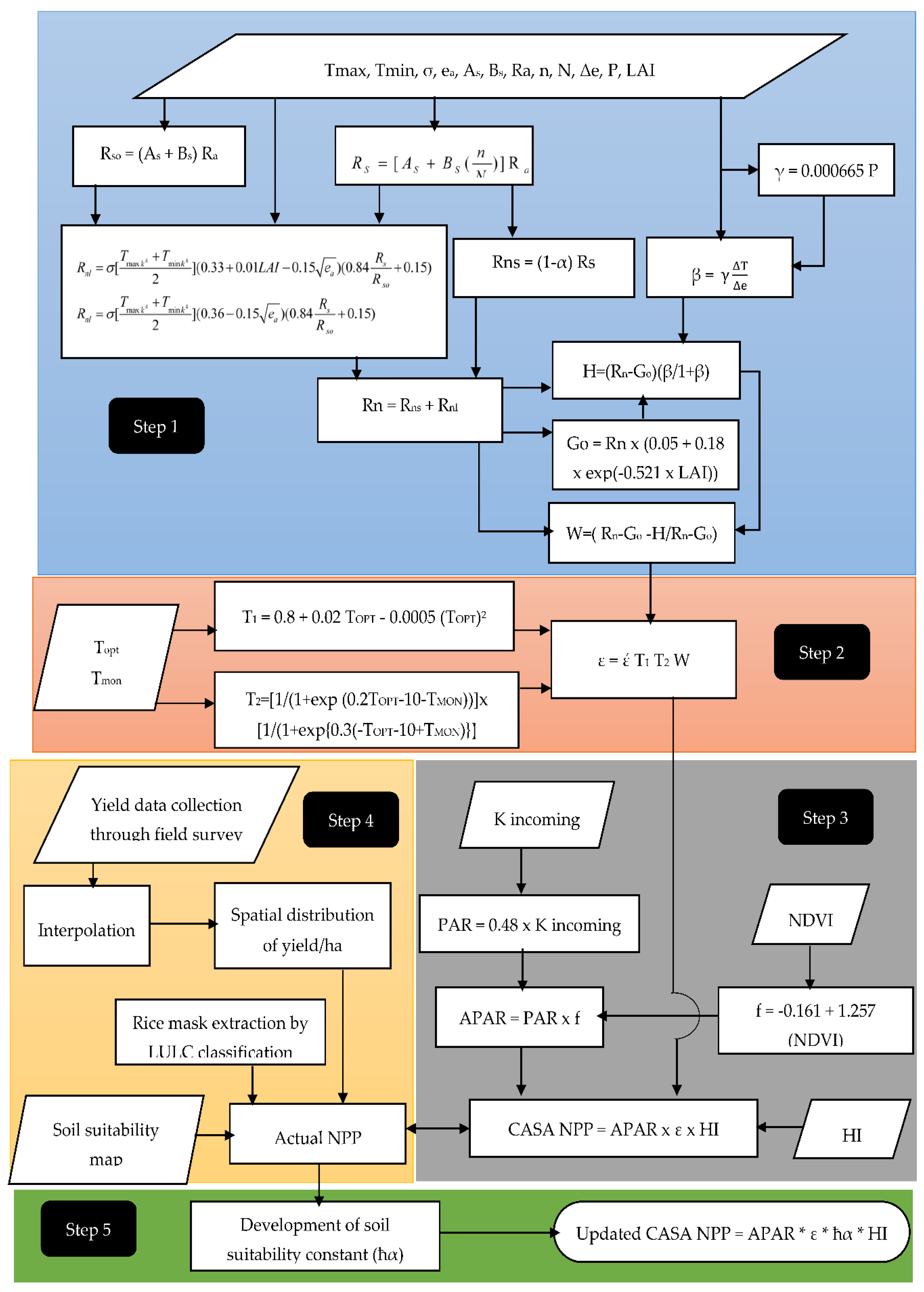
The methodology used in this research to estimate total rice production incorporating local ecological parameters, is described in detail with the flow chart shown in Figure 2 below.
2.3. CASA Model
We used the CASA model to examine the NPP in the investigation site. The CASA model is based on LUE, which is a commonly used index to model vegetation productivity at global scales [38,39,40,41] by fixing solar energy [42]. Estimation of LUE is an important and key parameter for mapping NPP that helps to spatially diagnose the vegetation health conditions. LUE is considered as an indispensable characteristic of plants [43] that show spatial heterogeneity at different scales due to composition of the species and plant physiological characteristics. At plant scale, LUE is influenced by many factors, including the amount of chlorophyll content, leaf age, intensity of the incident light and the plant growth stage [39]. However, at canopy scale, LUE is affected by canopy structure, solar zenith angle, leaf inclination angle and the LAI. Dissimilar vegetation types at the regional scale can be identified by computing spatial variability in LUE through remote-sensed data [44,45]. Several methods are available to compute LUE; these include the Eddy covariance technology method [46], productivity model inversion method [47] and quantum efficiency reckoning method [48,49]. During the last decade, site-based measurement was commonly used to compute LUE differences [50,51], however, the photochemical reflectance index [52,53,54,55] has been more widely used in recent years. LUE determines a positive relationship between NPP and absorbed photosynthetic active radiation (APAR). APAR can be computed using the (NDVI as input. The CASA model incorporates NDVI to compute the light absorption fraction of plants [26]. NDVI, a spectral index of crop canopy, relates linearly to the fraction of photosynthetic active radiation (PAR) intercepted by the crop canopy [56].
PAR is the portion of solar radiation between a wavelength range (0.4–0.7 µm) available for plants during the sunshine hours [57,58]. In the CASA model, NPP is calculated as a product of APAR and LUE [26,35,59,60,61] as represented in Equation (1).
NPP = APAR × ε (Kg/ha)
PAR is assigned a value ranging between 45% and 50% to represent averaged 24-h conditions [62] as in Equation (2).
where K24 is incoming solar radiation incident on crops during its growth period. The ratio of PAR and APAR represents the fraction ‘f’ of absorbed radiation in comparison to the available radiation for photosynthesis [44,63,64,65] and is computed in Equation (3).
PAR = 0.48 K24 (Wm−2)
APAR = f × PAR (Wm−2)
The fraction ‘f’ was estimated using NDVI values according to Field et al. (1995) [9] in Equation (4),
f = −0.161 + 1.257 (NDVI)
We obtained the Landsat satellite images listed in Table 1, to compute spatiotemporal variations in NDVI throughout the RCP.
LUE varies for various crops depending upon the physiological characteristics of the plants [42]. Asrar et al. (1985) [66] analyzed the impact of water stress on LUE. LUE results are maximal in ideal conditions and largely influenced by local temperature and moisture conditions. The LUE for rice crops was calculated as described in [9,35,43] Equation (5),
where έ determines the maximum conversion factor to compute biomass above the surface of the earth in optimal environmental conditions, and a value of 1.8 gC·MJ−1 is fixed for rice crops [67]. T1 and T2 are the heat factors and W is water stress on the crop throughout its growth. LUE will always be lower than έ [68]. T1 determines the impact of regional cold conditions, whereas T2 reveals that LUE decreases with deviations in actual crop temperature in comparison with the optimal temperature required for rice crop growth. T1 and T2 were computed according to [26,43,67].
where Topt is mean air temperature for the month with the maximum leaf area index (LAI) for a particular crop (e.g., we recorded maximum LAI for rice crops in the month of September), and Tmon is the mean monthly air temperature during the complete crop growth period. Variations in temperature were obtained for the complete RCP from LMOs located at district level and were averaged.
ε = έ T1 T2 W
T1 = 0.8 + 0.02 Topt − 0.0005 (Topt)2
T2 = [1/(1 + exp (0.2Topt-10 − Tmon))] × [1/(1 + exp{0.3( − Topt − 10 + Tmon)}]
W determines the amount of moisture content in the soil where the crop is sown [69]. A range of 0 to 1 is fixed for W, where 0 indicates an oven--dry soil while 1 indicates surplus of water [70]. In its early growth stages, rice crop need excess of water, that id, W > 0.5 which reduces to 0.1 before the ripening stage [71]. W is normally applied in fields to examine the soil wetness level and estimated according to [67],
where Rn is net radiation (Wm−2), Go is soil heat flux (Wm−2) and λE is the latent heat flux (Wm−2).
2.4. Net Radiation (Rn)
Rn is the key component of the earth’s energy balance that determines the ratio of incoming and outgoing radiations [72]. This energy balance closure affects the accuracy of the estimation of evapotranspiration, therefore, it is important to estimate Rn accurately to investigate the agroclimatic relationship [73]. Solar radiation is responsible for all physical and chemical processes occurring in the surface-atmosphere interface [74]. The physiological aspects of the rice crop canopy are computed using various parameters such as air temperature, leaf surface temperature, pressure, dew point, extraterrestrial radiation, actual sunshine hours, clear sky radiation, albedo and the actual vapor pressure [73,74,75,76,77,78,79,80,81]. Rn can be computed using these parameters at local and regional scales. Rn is the sum of the both incoming and outgoing shortwave (Rns) and longwave (Rnl) radiation [72,82,83]. Rn represents the balance between Rns and Rnl, computed as follows,
Rn = Rns + Rnl.
Rnl is four times proportional to the earth’s surface temperature, as stated by Stephen Boltzman law and computed according to [73].
where σ is the Stephen Boltzman constant (σ = 4.903 × 10⁻⁹ M J K−4 m−2 day−1), Tmaxk and Tmink are daily maximum and minimum temperature in Kelvin, ea is actual vapor pressure in KPa, Rs and Rso are incoming and actual/clear sky solar radiation (Wm−2). Daily variations in temperature (Tmaxk and Tmink) and ea for the complete RCP were obtained from LMOs and averaged.
The solar radiation striking at the top of the Earth’s atmosphere (TOA) is called extraterrestrial radiation (Ra) [84]. Ra changes throughout the year with the position of sun due to considerable variations in the solar incidence angle [85]. The fraction of Ra that actually approaches the surface of earth by interacting with the atmospheric gases is called incoming solar radiation (Rs), which depends mainly upon the cloud activity [85]. Rs was computed according to references [72,84,85,86,87,88,89].
where As and Bs are the calibration constants and a value range of 0.25 and 0.50 is recommended, respectively [85]. N and n are maximum and actual sunshine hours, respectively. The variations in N and n for the complete RCP were obtained by LMOs and averaged. Ra was computed by substituting the required parameters (latitude, month and day) in the website http://www.engr.scu.edu/~emaurer/tools/calc_solar_cgi.pl.
Clear sky radiation (Rso) is nearly 75% of Ra, which shows the fraction of radiation reaching the earth’s surface on cloud free days. The remaining 25% of Ra is absorbed, scattered or reflected back by atmospheric gases. Rso was computed using the Angstrom’s formula [84,86],
Rso = (As + Bs) Ra
Rns was computed by canopy surface albedo and incoming solar radiation according to [72,85].
where Rs is incoming solar radiation (Wm−2) calculated above in Equation (13) and α is albedo or the crop canopy reflection coefficient which is fixed for various crops e.g., albedo ranges between 0.15 and 0.25 for rice crops [90,91,92].
Rns = (1 − α) Rs
2.5. Soil Heat Flux Calculation (Go)
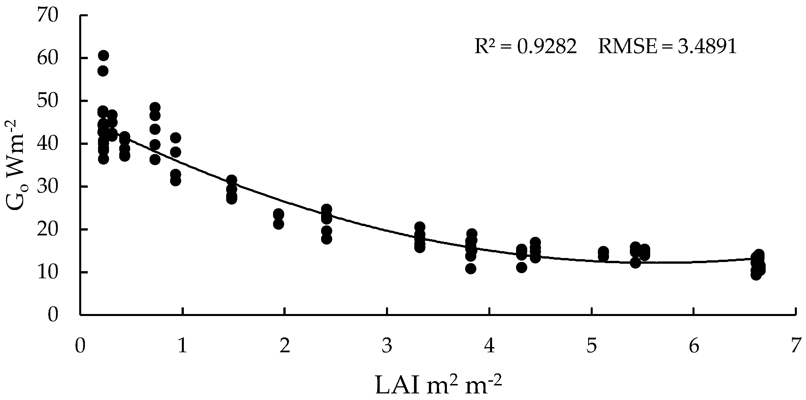
Go represents the conduction of heat in soil due to temperature gradient depending upon the soil characteristics [93]. Being a key factor, temperature controls all the biochemical processes in soil that are essential for plant growth [94]. Go has the smallest contribution in the energy balance equation, thus, it is often ignored but its exclusion may lead to considerable errors. Go was computed according to [95] as follows,
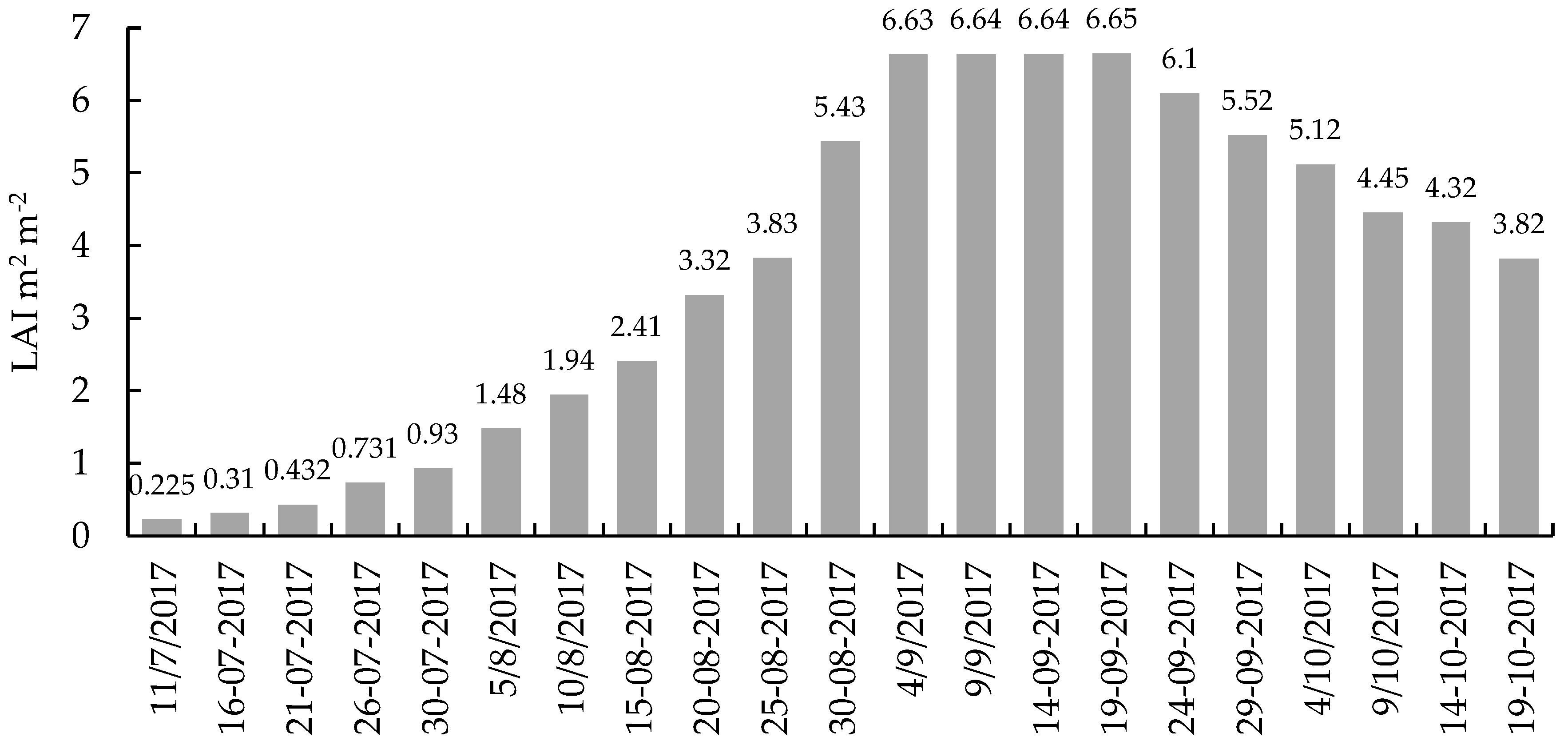
where Rn is net radiation and LAI is the leaf area index that varies throughout the crop growth. Estimation of LAI is important because Go largely depends upon the density of leaves through which heat penetrates to increase the soil temperature. We collected LAI values for the rice crops in various growth stages through 21 field observations using the instrument LAI 2200, these are mentioned in Figure 3. First observations regarding LAI were collected on 11 July 2017 and every five days thereafter and it was assumed that LAI remained relatively similar in the four days before the next observation was made, e.g., LAI was observed to be 0.225 m2 m−2 on 11 July 2017 and it was assumed to be the same for the next four days (12–15) July 2017.
Go = Rn × (0.05 + 0.18 × exp (−0.521 × LAI))
2.6. Latent (λE) and Sensible Heat Flux (H)
Sensible heat is the exchange of energy into the plant body without changing its state. It is important to accurately determine the proportion of sensible and latent heat flux, which is a difficult process [96,97]. Therefore, a residual of energy balance equation is used to compute evaporation over the vegetation surface and a Bowen ratio (β) is applied to compute sensible heat flux [98,99]. β can be computed using daily variations in temperature and actual vapor pressure for canopy-environment interface as follows,
where γ is a psychometric constant that is 0.000665 times the atmospheric pressure P [100]. ΔT and Δe are temperature and actual vapor pressure gradients, respectively. The expression for γ is as follows,
where P is daily atmospheric pressure in KPa. We collected ΔT, Δe and P from LMOs and averaged them. Sensible heat was computed using the Bowen ratio [99].
γ = 0.000665 × P
Latent heat flux is related to the estimation of crop canopy resistance which is difficult to measure because canopy resistance is dependent upon complex interactions (many times non-linear interactions) of plants with atmospheric factors [74]. Therefore, to avoid the canopy resistance method, the residual of energy balance equation was used to compute the latent heat flux [96,97,98,99,101,102,103,104] as follows,
λE = Rn − Go − H
2.7. Landsat Image Acquisition
Remotely sensed datasets are useful to extract spatial information (e.g., LAI and land cover type) to simulate carbon dynamics from regional to global scales [9,66]. Global carbon monitoring systems can be developed through ecosystem models driven using remotely sensed datasets [105]. We obtained five free Landsat 8 cloud images covering the complete RCP from the USGS, as mentioned in Table 1, to survey spatiotemporal variability for NDVI, APAR and biomass generation at the investigation site.
2.8. Supervised Classification
To estimate net production, it is important to accurately assess the area under rice cultivation. We performed Land Use Land Cover (LULC) supervised classification on Landsat 8 multispectral imagery (path 149, row 038) and applied various indices (NDVI, the normalized difference built-up index (NDBI) and the normalized difference water index (NDWI)) to get a classified map with high accuracy.
3. Results
3.1. Estimation of Solar Radiation Received by Rice Crop Canopy throughout the RCP
Solar radiation fluxes including clear sky radiation (Rso), actual incoming radiation (Rs), net radiation (Rn), net shortwave radiation (Rns) and net longwave radiation (Rnl) were computed by substituting the input parameters (T, ea, n, N, As, Bs and α collected through local LMOs) in Equations (9)–(14) and mapped the results in Figure 4.
Figure 4 shows the variations in Ra, Rso, Rs, Rn, Rns and Rnl throughout the RCP. Ra shows the maximum solar flux available at the TOA before entering into the earth’s atmosphere, whereas Rso is showing exactly the same pattern with a decline of 25% due to the interactions of Ra with atmospheric gases that results in 75% of Ra approaching the surface of earth. Ra was observed to be about 490.1 Wm−2 on 20 June 2017, which declined to 306.17 Wm−2 on 20 October 2017 due to a change in solar angle. The calculation of Ra, Rso and Rs determines that 52,409 Wm−2 was recorded at TOA as Ra, a fraction of which 39,307 Wm−2, 75% × Ra entered the earth’s atmosphere as Rso, however, 28,960 Wm−2 could be received as actual incoming solar radiation by the earth’s surface due to cloud activity at various spatial locations throughout the RCP. Rn was observed as 27,428 Wm−2, which included 4260 Wm−2 as Rnl and 23,168 Wm−2 as Rns. Rn is observed as 1532 Wm−2 less than Rs, the main reason of this difference is heat conduction in the soil as Go.
The variations in ratio (n/N) are mapped in Figure 5 which shows the ratio of actual sunshine hours in comparison to total sunshine hours. Careful estimates show that a total number of 1584 sunshine hours were available throughout the RCP out of which 966 sunshine hours could be received by the rice crop canopy. The main reason for this difference is the cloud activity at various locations in the study site throughout the RCP.
3.2. Estimation of Go throughout RCP
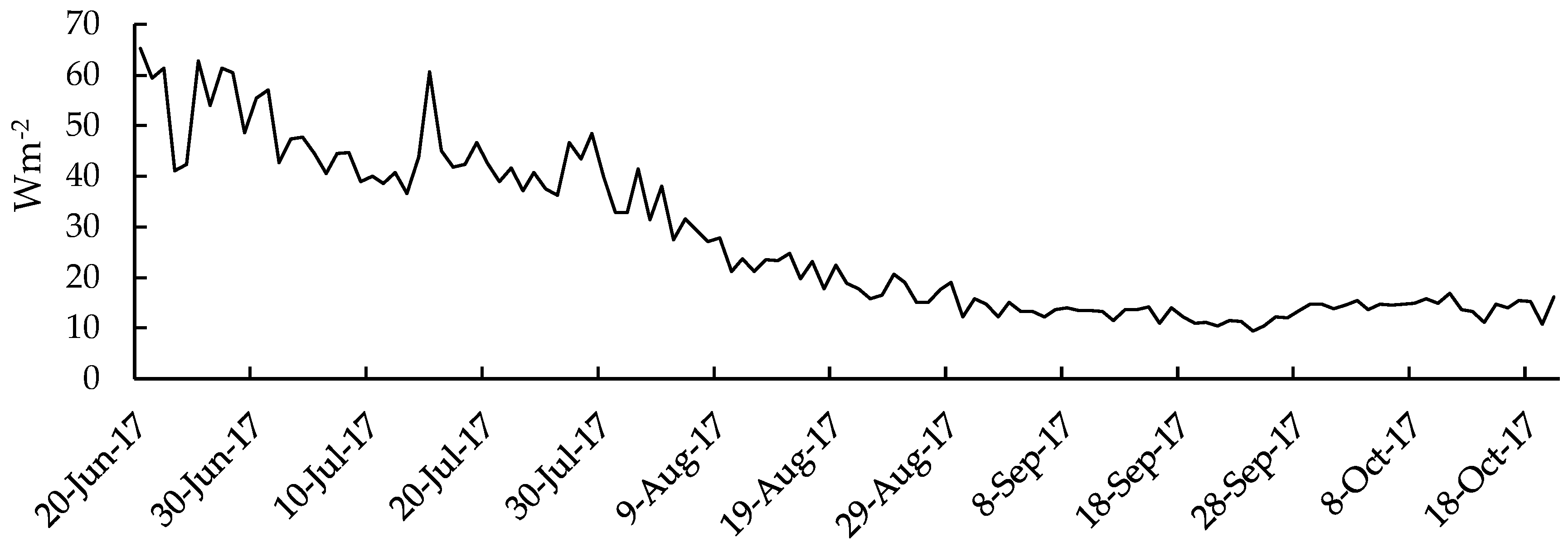
Variations in Go were estimated by substituting Rn and LAI (mentioned in Equation (15) and mapped the results in Figure 6. A gradually decreasing trend is observed in Go which fluctuated between (65.25–9.43) Wm−2 for the complete RCP. The gradual decline in Go is due to the increasing density of rice plant leaves over the growth period that prohibits the sunlight reaching the surface of earth for conduction processes.
3.3. Estimation of λE and H
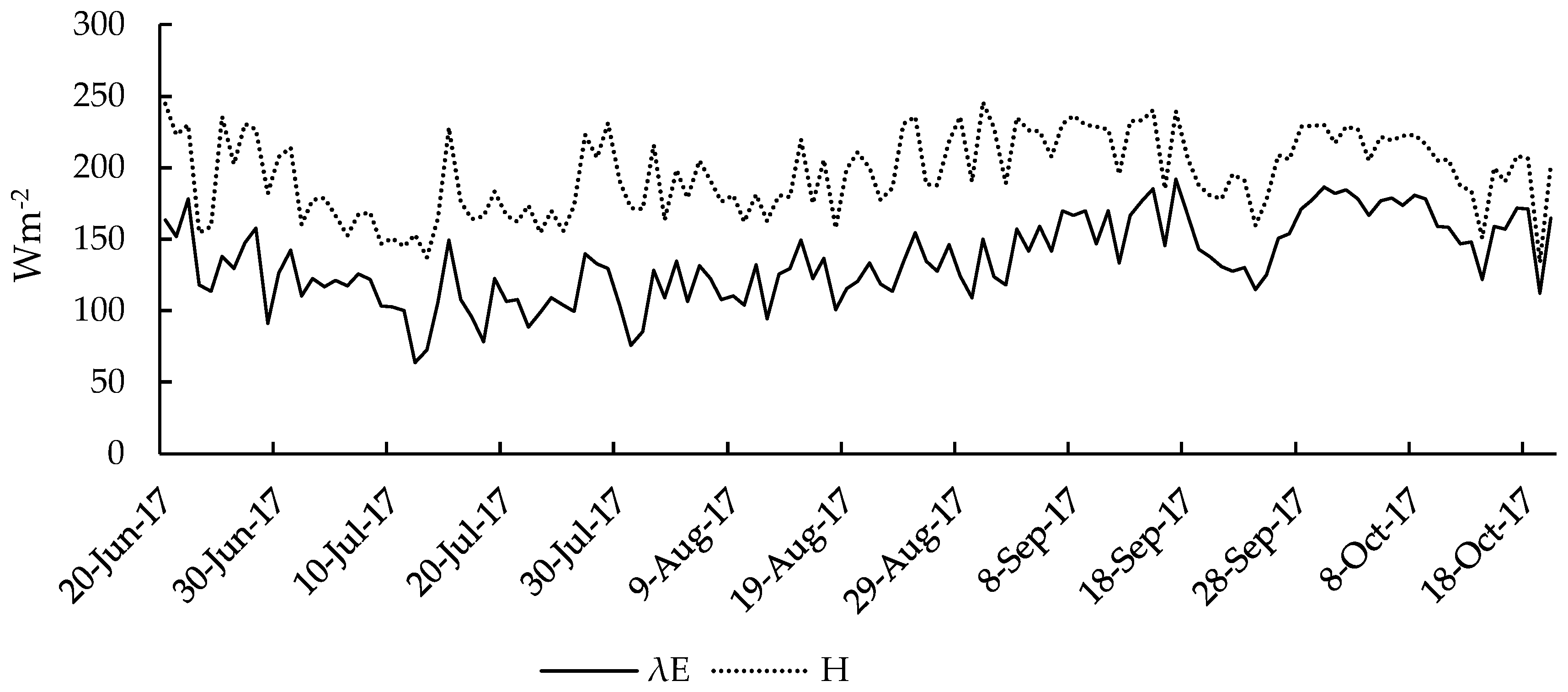
Figure 8 shows the variations in λE and H calculated through Equations (16)–(19) by incorporating T, P, Δe, Rn and Go on a daily basis throughout the RCP. Careful estimates show that 16,549 Wm−2 was taken by the rice crop canopy as H and 7554 Wm−2 was used for the transpiration process.
3.4. Estimation of W
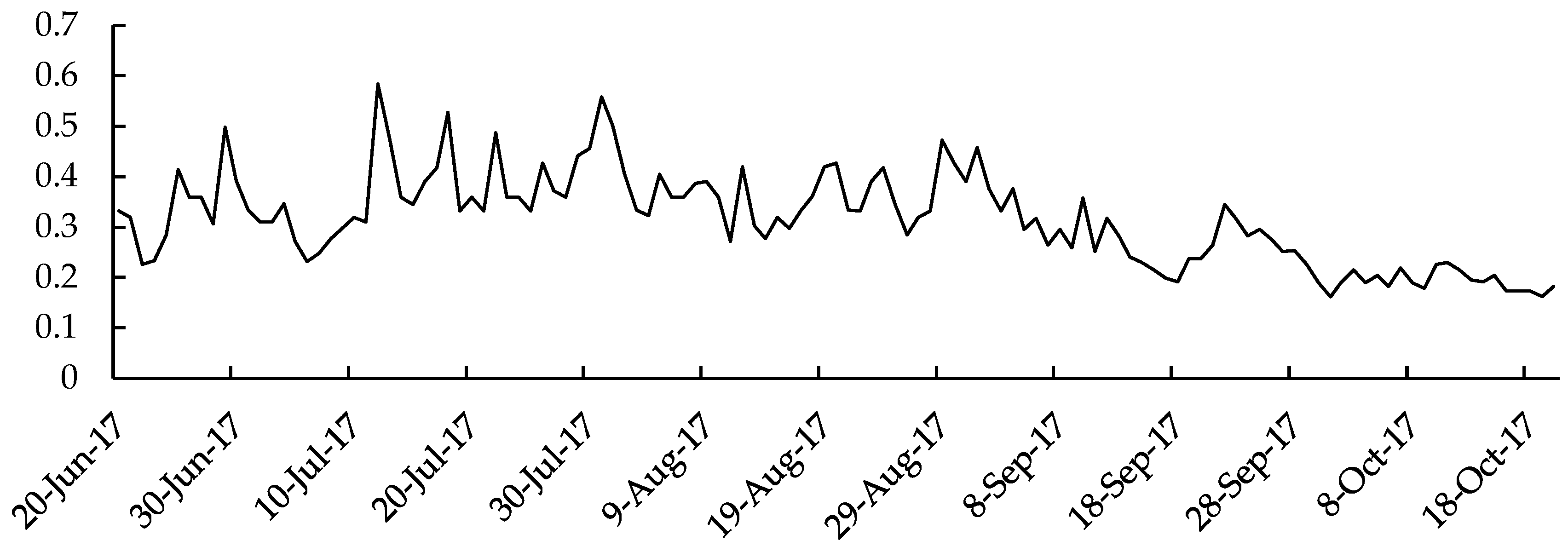
W indicates the transition between the dry and wet season. We estimated the variations in W and plotted the results in Figure 9 by substituting Rn, Go and H in Equation (8). It shows a decreasing trend from the start to the end of the RCP. W fluctuated between 0.5838 and 0.1218 in our study site, which reflects the water surplus and water deficiency scenarios, respectively.
3.5. Estimation of LUE
The light used by the rice crop canopy was estimated on a daily basis by substituting έ = 1.8 gC·MJ−1 in Equation (5) and the results are plotted in Figure 10. Maximum light intake by the rice crop canopy was observed in the early growth stages while a decreasing trend was observed toward the ripening stage or on the days with cloud activity.
3.6. Biomass/NPP Estimation
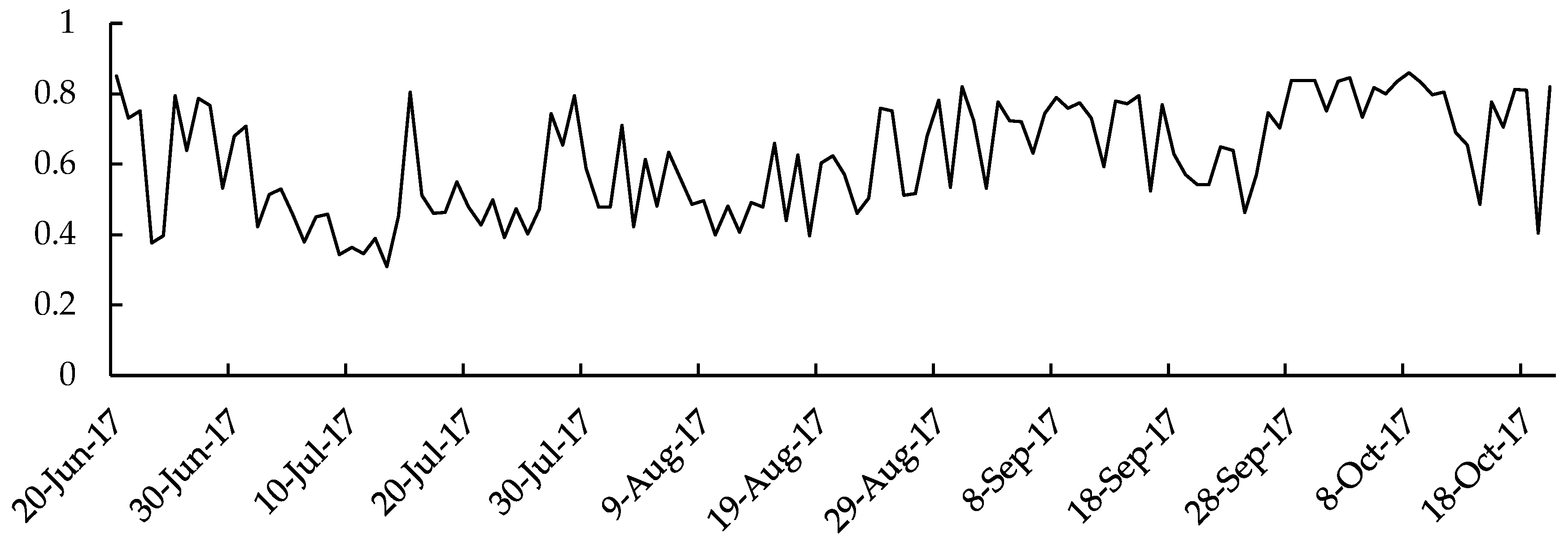
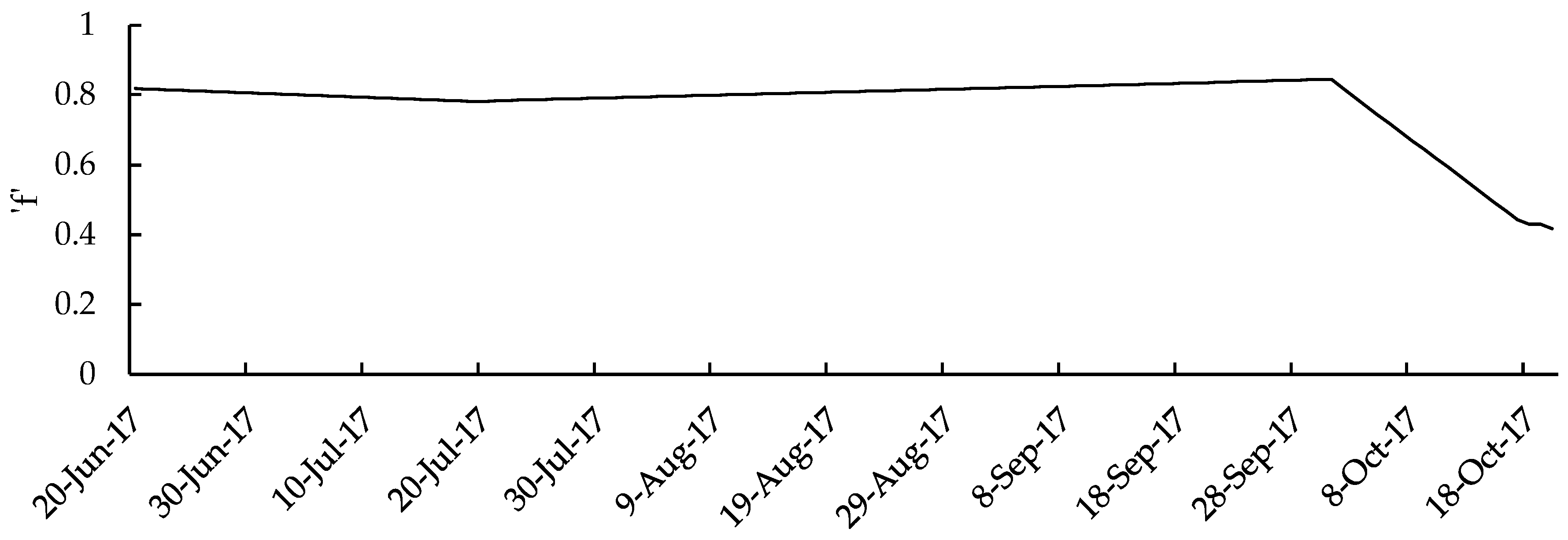
To estimate biomass, the input parameter ‘f’, ‘PAR’ and ‘APAR’ were computed. To calculate ‘f’, daily variations in NDVI throughout the RCP were substituted in Equation (4) and the results are plotted in Figure 11. ‘f’ varies between 0 and 1 which determines the fraction of PAR used by rice crop canopy for photosynthesis as APAR. If ‘f’ = 0, it means that APAR is nil, while 1 depicts that APAR = PAR. Figure 11 shows a sharp decline in ‘f’ on 1 October 2017 because the rice crop turned to yellow at the ripening stage on this date. APAR is directly affected by NDVI, a decrease in NDVI leads to a drop in APAR and vice versa.
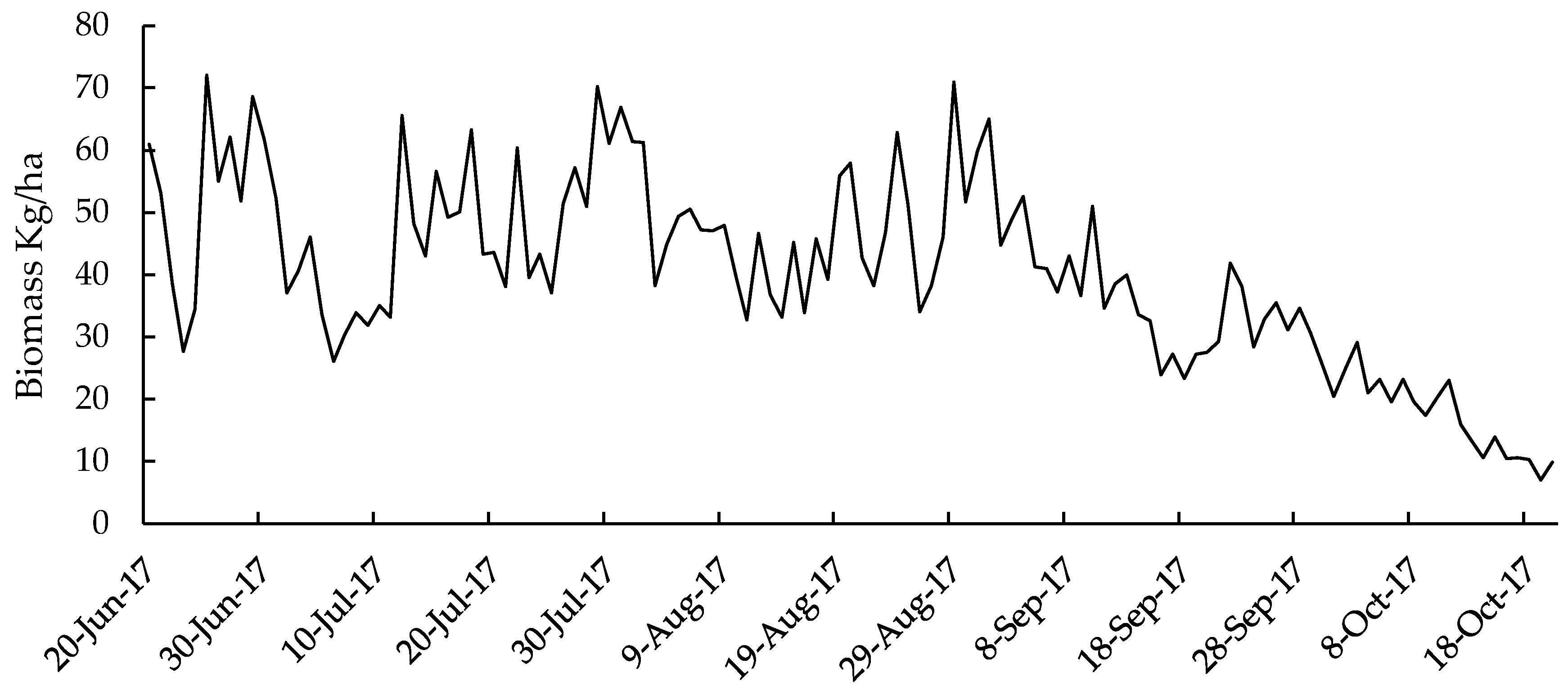
We estimated biomass generation on a daily basis by substituting APAR and ε values in Equation (1) and the results are plotted in Figure 12. Biomass generation declined as NDVI dropped at the ripening stage mentioned in Figure 11, during the month of October. The decline in NDVI directly affects both the APAR and ε, because rice plants need comparatively less energy at the ripening stage as compared to its overall growth stages, consequently, APAR and ε dropped even in cloud free October. Peaks and dips in Figure 12 describe sunlight (n/N ratio) available for APAR and ε that directly affects the biomass potency.
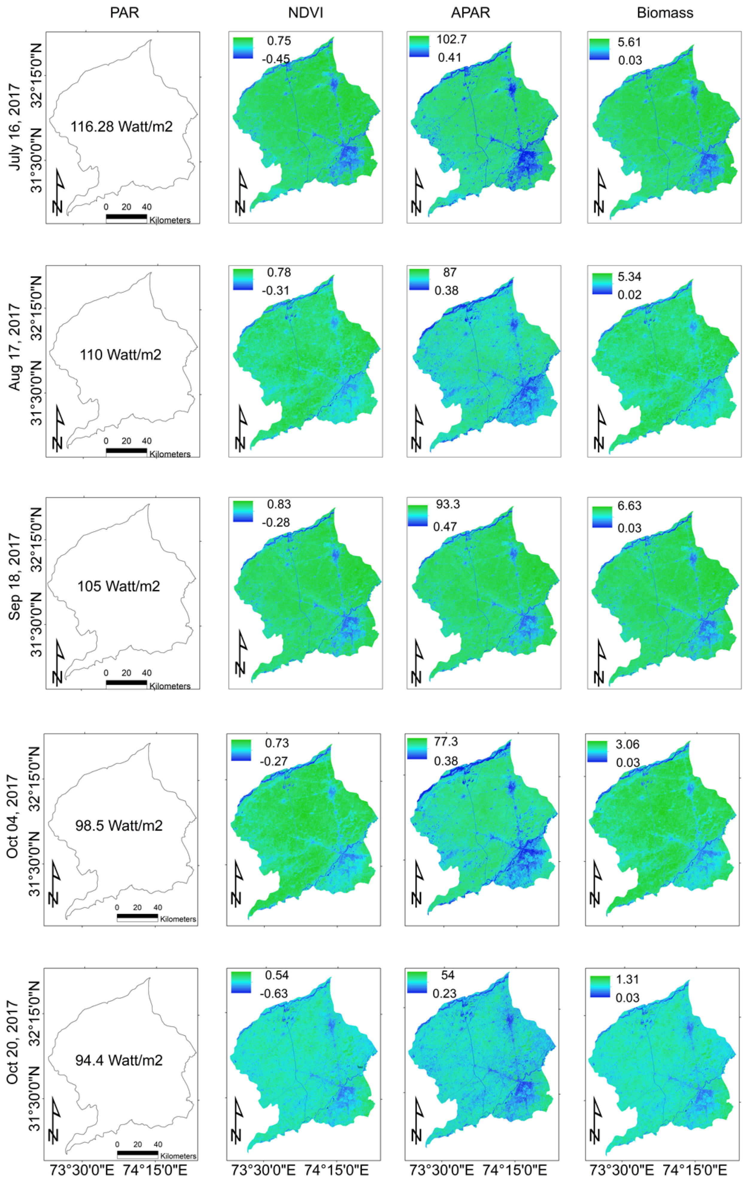
Landsat 8, remotely sensed datasets listed in Table 1, were used to survey spatiotemporal variations in PAR, APAR, NDVI and biomass generation and the results are mapped in Figure 13. Lush green areas in Figure 13 determine the spatial extent of vegetation while blue areas represent non-vegetative features.
Careful estimates revealed that 4897 kg/ha biomass is generated in the study site throughout the RCP. The harvest index for rice crops is taken as 0.50 [106], which resulted in a dry mass of 2450 kg/ha (2.7 ton/ha). To compute net production, we extracted the area under rice cultivation through supervised classification. The classification results show that the total area under investigation was 13,680 km2, of which 8861 km2 (886,100 ha) was under rice cultivation. A field survey was conducted along with Maali patwari (a local expert) to cross validate the classification results which were 92.35% accurate. According to international standards the reliability of supervised neighborhood classification may be up to 94% [107]. The net rice production was approximated as 2.39 million tons.
4. Discussion
Ratio (n/N) determines the cloud activity, which ranges between 0 and 1 (0 indicates a dense cloudy day and 1 is a cloud free day). This ratio has a direct impact on all productivity parameters e.g., Rns, Rnl, Rn, Rs, H, λE, LUE as well as the biomass generation. The peaks and dips in Figure 4, Figure 6, Figure 8, Figure 10 and Figure 12 show the same pattern as the (n/N) ratio in Figure 5. A decline in (n/N), for example, 0.5 determines that half of the day is without sunshine and this results in a drop in observed Rn, Rns, Rnl and Rs. Rs is equivalent to Rso on the day (where n = N). LUE is directly affected by the (n/N) ratio because it limits the sunlight falling on the rice crop canopy, therefore, photosynthesis/respiration process is halted or delayed. Ratio (n/N) can be significant or insignificant during various stages of rice crop growth (e.g., leaf emergence and tillering processes need comparatively high temperatures for proper growth where (n/N) ratio is feasible and near to 1), besides, the flowering, milk, dough and ripening stages remain good at lower temperatures when the (n/N) ratio should be less than 0.5. Figure 8, shows a decline for both λE and H for the days with partial or full cloud activity because less energy is required to maintain the plant internal temperature as compared to its surroundings. Go is also affected by the ratio (n/N) as shown in Figure 6, e.g., the dip in Go in Figure 5 on 24 July 2017 describes the dense cloud activity, which resulted in the non-availability of heat for conduction through the soil. Figure 6 shows that Go was comparatively high in the early growth stages due to less LAI as compared to forthcoming growth stages.
The difference in Rn and Go is equivalent to the collective impact of λE and H on the rice crop canopy. λE and H are directly affected by the ratio (n/N). H is the transfer of heat to a rice plant to maintain its internal temperature according to the ambient air. λE is the energy consumption for the transpiration process. Temperature drops on a cloudy day due to non-availability of direct sunlight and hence less energy is consumed for both the λE and H.
W indicates the soil wetness level which ranges between 0 and 1. Temporal variations in W were mapped in Figure 9 and determine the soil wetness condition throughout the RCP. Rice crops in the form of green biomass in various growth stages had high concentration of water i.e., (W ≥ 0.5). W declined in the same way as green biomass turned to yellow during the final ripening stage and reached a level of 0.1218. W = 0 indicates that the rice plant is oven-dry. The same results for water stress were obtained by [9]. T1 and T2 expresses the regulation of rice plants by temperature. Light used by the rice crop canopy may not be well computed, if these key parameters are ignored. T2 represents the variations in the temperature regulation on the rice crop throughout the RCP while T1 incorporates the impact of temperature fluctuations during the month with LAI max. LAI max was obtained through field observations that varied between (6.63–6.65) m2 m−2 during the month of September 2017 with an optimum temperature of 30.5 °C. T2 becomes 1 if Topt and Tmon are equal to each other. T2 = 0.5 determines that Tmon differs with Topt by 10–15 °C. Topt and Tmon were observed as slightly different from each other in our study site, however, significant variations in Topt and Tmon may be observed by investigating agricultural productivity at a continental scale. The fraction ‘f’ of absorbed radiation in comparison to available radiation is mapped in Figure 11. This shows that about 80% of incoming radiation was used by the rice crop canopy and this suddenly dropped on 1 October 2017. This sharp decline was due to a decrement in NDVI on the same day, therefore, the reflective index of the rice crop canopy (NDVI) is an important parameter of productivity. As NDVI drops, the LUE of the plant declines and hence the biomass generation decreases regardless of weather conditions, as shown in Figure 10, Figure 11 and Figure 12. The collective impact of all the parameters of productivity are mapped in Figure 12. There was a resemblance in Figure 5 and Figure 12 which determines that the (n/N) ratio directly affects rice productivity. Figure 13 shows the spatiotemporal variations in PAR, APAR, NDVI and biomass generation. The lowest values in NDVI, APAR and biomass datasets reveal various features (e.g., a built-up area, a water body and some non-cropped and salinized land) other than green biomass. A gradual decreasing trend is observed in PAR values from July to October due to a change in sun inclination angle. NDVI was recorded as maximum in the month of September due to increased LAI; this suddenly declined in October in the ripening stage. Maximum NDVI results in enhanced biomass generation therefore, there is a direct relationship between NDVI and biomass generation. Biomass generation was observed least in October because the rice crop was in the ripening stage during that time. APAR was observed as maximal in the early growth stages of the rice plant because an increased growth is observed at the same time due to the emergence of leaves and tillering. APAR degraded in October because the rice crop turned yellow because photosynthesis was partially halted, even during sunshine hours.
Development of Soil Suitability Constant (ħα)
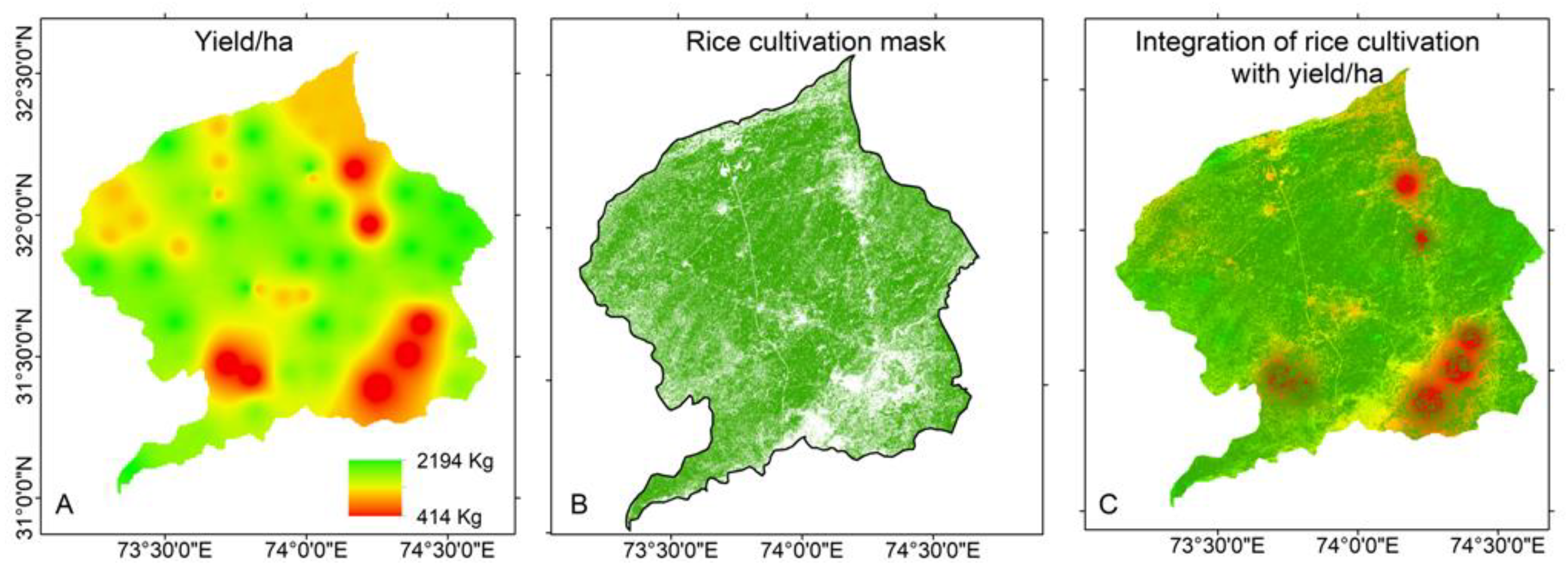
Actual yield levels were obtained through 55 field observations taken randomly by interviewing local farmers. The observations sites were chosen keeping in mind the diversity in yield reported by farmers at rice monitoring centers. High variations were observed between actual (obtained through the field survey) and estimated (using the CASA model) yields. We obtained four ranges of actual yield, which were 400–500 kg/ha, 1000–1200 kg/ha, 1700–1800 kg/ha and 2100–2200 kg/ha. These ranges were 0.16–0.2%, 0.4–0.48%, 0.69–0.73% and 0.85–0.90% of the CASA based yield, respectively. To investigate further, an interpolated map was developed based on actual yield levels, as shown in Figure 14, and it was compared with soil suitability zones delineated by Hassan et al., 2018 [108]. We observed that the lowest yield of 414 kg/ha (0.16% of the CASA based yield) was obtained from areas which were not suitable for rice cultivation with pH > 8.4, electric conductivity (EC) of 1.75–2.25 and excessively drained soil type (ST). In addition, for the other three yield ranges the following results were obtained: (1) 1100–1200 kg/ha with soil suitability levels, pH = 4–5, EC = 1.75–2.25 and highly drained ST; (2) 1700–1800 kg/ha with soil suitability levels, pH = 7.7–8.3, EC = 0.25–0.75 and well drained ST; and (3) 2100–2200 kg/ha with soil suitability levels, pH = 5.5–7.2, EC = 0.75–1.50 and poorly drained ST. The CASA model demonstrates wide differences between actual and estimated yield [33,34,44,64,67,68] because it ignores soil suitability levels that must be incorporated to obtain precise yield. So, we developed a soil suitability constant, denoted as ħα, on the basis of our results. The values of ħα ranges between 0.05 and 0.95. We further subdivided it into four ranges; 0.05–0.25 for not suitable, (0.4–0.6) for less suitable, (0.7–0.75) for moderately suitable and (0.85–0.95) for highly suitable soil types. These ħα based levels can be applied only if one has delineated cultivation sites based on physical and ecological grounds. The refining of ħα can improve the CASA based NPP. Finally, the improved method for computing NPP through the CASA model with the addition of ħα is given as,
Net Productions = APAR ∗ ε ∗ ħα ∗ HI (Kg/ha)
There were other ground validations that caused an over estimation in yield, which were: (1) non-availability of open-source satellite images with high spatiotemporal resolution to determine growth variability on a daily basis; (2) poverty and water scarcity faced by local farmers; (3) lack of state-of-the-art technology, poor agricultural and educational practices; and (4) blind faith of farmers on the crop calendar, which has now become obsolete due to existing phenological changes.
We further superimposed the spatial distribution of rice cultivation to yield a variability map (already compared with soil suitability zones), [108] and found that the farmers had planted rice in 592 km2 of less suitable soil, in 4385 km2 of highly suitable soil, in 2210 km2 of moderately suitable soil, and in 1674 km2 of not suitable soil. We applied ħα ranges according to soil suitability zones and computed 1.63 million tons as the net production in the study site, including 0.46 ton/ha for the not suitable zone, 1.2 ton/ha for the less suitable zone, 1.9 ton/ha for the moderately suitable zone and 2.4 ton/ha for the highly suitable zone.
5. Conclusions
Remote sensing has become a useful tool for monitoring NPP and biomass generation. Remotely sensed datasets are of great importance to repeatedly monitor agricultural productivity. This research was conduction through the CASA model in collaboration with freely available Landsat imagery that approximated the rice productivity, resulted in significant differences as compared to actual estimates. The differences in productivity were due to the soil suitability zones being ignored, thus, we added a new soil suitability constant (ħα).
This research can be applied to surveys of spatiotemporal variations in yield that require actual sunshine hours, temperature, actual vapor pressure, rate of change in leaf area and the air pressure on a daily basis. This research opens avenues to investigate ħα ranges in detail.
Author Contributions
S.M.H.R. and S.A.M. generated the complete flow of methodology used in this research and arranged data on a daily basis from LMOs, rice monitoring centers and by local farmers. S.A.M. arranged funds and conducted field surveys for ground truthing. S.M.H.R. and S.A.M. produced the results and discussed with. A.A.K. (MNSUM) who checked the whole flow of the research. He also helped in reviewing this research by his three associates living in Germany, Brazil and Indonesia, regarding English related issues.
Acknowledgments
We are thankful to the Vice Chancellor of the University of the Punjab for providing us financial support to conduct this research. Alamgir A Khan (MNSUM) and various rice monitoring centers existing in the study site, for their fully-fledged cooperation. We also thank USGS for providing us their valuable satellite data freely to accomplish this research.
Conflicts of Interest
The authors declare no conflict of interest.
References
- Mosleh, M.K.; Hassan, Q.K.; Chowdhury, E.H. Development of Remote Sensing Based Rice Yield Forecasting Model. Span. J. Agric. Res. 2016, 14, 3. [Google Scholar] [CrossRef]
- Yang, C.M.; Liu, C.C.; Wang, Y.W. Using FORMOSAT-2 satellite data to estimate leaf area index of rice crop. J. Photogram. Remote Sens. 2008, 13, 253–260. [Google Scholar]
- The Statistics Portal. Paddy Rice Production Worldwide in 2017, by Country (in Million Metric Tons). Available online: https://www.statista.com/statistics/255937/leading-rice-producers-worldwide/ (accessed on 5 December 2017).
- Huang, J.-F.; Tang, S.-C.; Ousama, A.-I.; Wang, R.-C. Rice yield estimation using remote sensing and simulation. J. Zhejiang Univ. Sci. A 2002, 3, 461–466. [Google Scholar] [CrossRef]
- USDA. World Agricultural Production. Foreign Agricultural Service. Available online: http://www.fas.usda.gov/psdonline/psdreport.aspx?hidReportRetrievalName=BVS&hidReportRetrievalID=893&hidReportRetrievalTemplateID=1 2013 (accessed on 12 November 2017).
- Xiao, X.; Boles, S.; Liu, J.; Zhuang, D.; Frolking, S.; Li, C.; Salas, W.; Moore, B., III. Mapping paddy rice agriculture in southern China using multi-temporal MODIS images. Remote Sens. Environ. 2005, 95, 480–492. [Google Scholar] [CrossRef]
- Reynolds, C.A.; Yitayew, M.; Slack, D.C.; Hutchinson, C.F.; Huete, A.; Petersen, M.S. Estimation crop yields and production by integrating the FAO crop specific water balance model with real-time satellite data and ground-based ancillary data. Int. J. Remote Sens. 2000, 21, 3487–3508. [Google Scholar] [CrossRef]
- Zhu, Q.; Zhao, J.; Zhu, Z.; Zhang, H.; Zhang, Z.; Guo, X.; Bi, Y.; Sun, L. Remotely Sensed Estimation of Net Primary Productivity (NPP) and Its Spatial and Temporal Variations in the Greater Khingan Mountain Region, China. Sustainability 2017, 9, 1213. [Google Scholar] [CrossRef]
- Field, C.B.; Randerson, J.T.; Malmström, C.M. Global Net Primary production: Combining ecology and Remote sensing. Remote Sens. Environ. 1995, 51, 74–88. [Google Scholar] [CrossRef]
- Lima, E.D.P.; Sediyama, G.C.; Silva, B.B.D.; Gleriani, J.M.; Soares, V.P. Seasonality of net radiation in two sub-basins of Paracatu by the use of MODIS sensor products. Eng. Agric. 2012, 32, 1184–1196. [Google Scholar] [CrossRef]
- Liu, G.S.; Liu, Y.; Xu, D. Comparison of evapotranspiration temporal scaling methods based on lysimeter measurements. J. Remote Sens. 2011, 15, 270–280. [Google Scholar]
- Pachavo, G.; Murwira, A. Remote sensing net primary productivity (NPP) estimation with the aid of GIS modelled shortwave radiation (SWR) in a Southern African Savanna. Int. J. Appl. Earth Obs. Geoinform. 2014, 30, 217–226. [Google Scholar] [CrossRef]
- Scurlock, J.M.; Johnson, K.; Olson, R.J. Estimating net primary productivity from grassland biomass dynamics measurements. Glob. Chang. Biol. 2002, 8, 736–753. [Google Scholar] [CrossRef]
- Maselli, F.; Argenti, G.; Chiesi, M.; Angeli, L.; Papale, D. Simulation of grassland productivity by the combination of ground and satellite data. Agric. Ecosyst. Environ. 2013, 165, 163–172. [Google Scholar] [CrossRef]
- Wang, P.J.; Xie, D.H.; Zhou, Y.Y.; E, Y.H.; Zhu, Q.J. Estimation of net primary productivity using a process-based model in Gansu Province, Northwest China. Environ. Earth Sci. 2014, 71, 647–658. [Google Scholar] [CrossRef]
- Canadell, J.G.; Mooney, H.A.; Baldochi, D.D.; Berry, J.A.; Ehleringer, J.R.; Field, C.B.; Gower, S.T.; Hollinger, D.Y.; Hunt, J.E.; Jackson, R.B.; et al. Carbon metabolism of the terrestrial biosphere: A multi-technique approach for improved understanding. Ecosystems 2000, 3, 115–130. [Google Scholar] [CrossRef]
- Piao, S.L.; Fang, J.Y.; He, J. Variations in vegetation net primary production in the Qinghai—Xizang plateau, China, from 1982 to 1999. Clim. Chang. 2006, 74, 253–267. [Google Scholar] [CrossRef]
- Eisfelder, C.; Klein, I.; Niklaus, M.; Kuenzer, C. Net primary productivity in Kazakhstan, its spatio-temporal patterns and relation to meteorological variables. J. Arid Environ. 2014, 103, 17–30. [Google Scholar] [CrossRef]
- Cramer, W.; Kicklighter, D.W.; Bondeau, A.; Moore, B., III; Churkina, G.; Nemry, B.; Ruimy, A.; Schloss, A.L. Comparing global models of terrestrial net primary productivity (NPP): Overview and key results. Glob. Chang. Biol. 1999, 5 (Suppl. 1), 1–15. [Google Scholar] [CrossRef]
- Lehuger, S.; Gabrielle, B.; Cellier, P.; Loubet, B.; Roche, R.; Béziat, P.; Ceschia, E.; Wattenbach, M. Predicting the net carbon exchanges of crop rotations in Europe with an agro-ecosystem model. Agric. Ecosyst. Environ. 2010, 139, 384–395. [Google Scholar] [CrossRef]
- Lauenroth, W.K.; Wade, A.A.; Williamson, M.A.; Ross, B.E.; Kumar, S.; Cariveau, D.P. Uncertainty in calculations of net primary production for grasslands. Ecosystems 2006, 9, 843–851. [Google Scholar] [CrossRef]
- Lin, H.L.; Feng, Q.S.; Liang, T.G.; Ren, J.Z. Modelling global-scale potential grassland changes in spatio-temporal patterns to global climate change. Int. J. Sustain. Dev. World Ecol. 2013, 20, 83–96. [Google Scholar] [CrossRef]
- Lin, H.L. A New Model of Grassland Net Primary Productivity (NPP) Based on the Integrated Orderly Classification System of Grassland. In Proceedings of the Sixth International Conference on Fuzzy Systems and Knowledge Discovery, Tianjin, China, 14–16 August 2009; pp. 52–56. [Google Scholar]
- Lieth, H. Modeling the primary productivity of the world. Nat. Resour. 1972, 8, 5–10. [Google Scholar]
- Potter, C. Microclimate influences on vegetation water availability and net primary production in coastal ecosystems of Central California. Landsc. Ecol. 2014, 29, 677–687. [Google Scholar] [CrossRef]
- Potter, C.S.; Randerson, J.T.; Field, C.B.; Matson, P.A.; Vitousek, P.M.; Mooney, H.A.; Klooster, S.A. Terrestrial ecosystem production: A process model based on global satellite and surface data. Glob. Biogeochem. Cycles 1993, 7, 811–841. [Google Scholar] [CrossRef]
- Liang, W.; Yang, Y.T.; Fan, D.M.; Guan, H.D.; Zhang, T.; Long, D.; Zhou, Y.; Bai, D. Analysis of spatial and temporal patterns of net primary production and their climate controls in China from 1982 to 2010. Agric. For. Meteorol. 2015, 204, 22–36. [Google Scholar] [CrossRef]
- Hicke, J.A.; Asner, G.P.; Randerson, J.T.; Tucker, C.; Los, S.; Birdsey, R.; Jenkins, J.C.; Field, C.; Holland, E. Satellitederived increases in net primary productivity across North America, 1982–1998. Geophys. Res. Lett. 2002, 29, 69-1–69-4. [Google Scholar] [CrossRef]
- Tang, C.J.; Fu, X.Y.; Jiang, D.; Fu, J.Y.; Zhang, X.Y.; Zhou, S. Simulating spatiotemporal dynamics of Sichuan grassland net primary productivity using the CASA model and in situ observations. Sci. World J. 2014, 10, 1–12. [Google Scholar] [CrossRef] [PubMed]
- Piao, S.L.; Fang, J.Y.; Zhou, L.M.; Zhu, B.; Tan, K.; Tao, S. Changes in vegetation net primary productivity from 1982 to 1999 in China. Glob. Biogeochem. Cycles 2005, 19, GB2027. [Google Scholar] [CrossRef]
- Liu, S.N.; Zhou, T.; Wei, L.Y.; Shu, Y. The spatial distribution of forest carbon sinks and sources in China. Chin. Sci. Bull. 2012, 57, 1699–1707. [Google Scholar] [CrossRef]
- Yu, D.Y.; Zhu, W.Q.; Pan, Y.H. The role of atmospheric circulation system playing in coupling relationship between spring NPP and precipitation in East Asia area. Environ. Monit. Assess. 2008, 145, 135–143. [Google Scholar]
- Rui, S.; Zhu, Q. Estimation of net primary productivity in China using remote sensing data. J. Geograph. Sci. 2001, 11, 14–23. [Google Scholar] [CrossRef]
- Piao, S.L.; Fang, J.Y.; Guo, Q.H. Application of CASA model to the estimation of Chinese terrestrial net primary productivity. Chin. J. Plant Ecol. 2001, 25, 603–608. [Google Scholar]
- Li, A.; Bian, J.; Lei, G.; Huang, C. Estimating the Maximal Light Use Efficiency for Different Vegetation through the CASA Model Combined with Time-Series Remote Sensing Data and Ground Measurements. Remote Sens. 2012, 4, 3857–3876. [Google Scholar] [CrossRef]
- Chen, L.J.; Liu, G.H.; Li, H.G. Estimating Net Primary Productivity of Terrestrial Vegetation in China Using Remote Sensing. J. Remote Sens. 2002, 6, 129–135. [Google Scholar]
- Waqar, M.M.; Rehman, F.; Ikram, M. Land suitability assessment for rice crop using geo spatial techniques. In Proceedings of the 2013 IEEE International, Geoscience and Remote Sensing Symposium (IGARSS), Melbourne, VIC, Australia, 21–26 July 2013. [Google Scholar]
- Wang, H.; Li, X.; Long, H.; Zhu, W. A study of the seasonal dynamics of grassland growth rates in Inner Mongolia based on AVHRR data and a light-use efficiency model. Int. J. Remote Sens. 2009, 30, 3799–3815. [Google Scholar] [CrossRef]
- Brogaard, S.; Runnstrom, M.; Seaquist, J.W. Primary production of Inner Mongolia China, between 1982 and 1999 estimated by a satellite data-driven light use efficiency model. Glob. Planet. Chang. 2005, 45, 313–332. [Google Scholar] [CrossRef]
- As-Syakur, A.R.; Osawa, T.; Adnyana, I.W.S. Medium spatial resolution satellite imagery to estimate gross primary production in an urban area. Remote Sens. 2010, 2, 1496–1507. [Google Scholar] [CrossRef]
- Propastin, P.; Kappas, M. Modeling Net Ecosystem exchange for grassland in Central Kazakhstan by combining remote sensing and field data. Remote Sens. 2009, 1, 159–183. [Google Scholar] [CrossRef]
- Monteith, J.L. Solar radiation and productivity in tropical ecosystems. J. Appl. Ecol. 1972, 9, 747–766. [Google Scholar] [CrossRef]
- Bradford, J.B.; Hicke, J.A.; Lauenroth, W.K. The relative importance of light-use efficiency modifications from environmental conditions and cultivation for estimation of large-scale net primary productivity. Remote Sens. Environ. 2005, 96, 246–255. [Google Scholar] [CrossRef]
- Ahl, D.E.; Gower, S.T.; Mackay, D.S.; Burrows, S.N.; Norman, J.M.; Diak, G.R. Heterogeneity of light use efficiency in a northern Wisconsin forest: Implications for modeling net primary production with remote sensing. Remote Sens. Environ. 2004, 93, 168–178. [Google Scholar] [CrossRef]
- Zhu, W.; Pan, Y.; He, J.; Yu, D.; Hu, H. Simulation of maximum light use efficiency for some typical vegetation types in China. Chin. Sci. Bull. 2006, 51, 457–463. [Google Scholar] [CrossRef]
- Xiao, X.; Zhang, Q.; Scott, S. Satellite-based modeling of gross primary production in a seasonally moist tropical evergreen forest. Remote Sens. Environ. 2005, 94, 105–122. [Google Scholar] [CrossRef]
- Pei, B.; Yuan, Y.; Jia, Y.; Wang, W.; Josef, E. A study on light utilization of poplar crop intercropping system. Sci. Silvae Sin. 2000, 36, 13–18. [Google Scholar]
- Zhu, Z.; Zhang, F. Solar energy utilization efficiency of the land plants in China. Acta Ecol. Sin. 1985, 5, 343–355. (In Chinese) [Google Scholar]
- Zhang, M.; Yu, G.; Zhuang, J.; Gentry, R.; Fu, Y.; Sun, X.; Zhang, L.; Wen, X.; Wang, Q.; Han, S.; et al. Effects of cloudiness change on net ecosystem exchange, light use efficiency, and water use efficiency in typical ecosystems of China. Agric. For. Meteorol. 2011, 151, 803–816. [Google Scholar] [CrossRef]
- Jenkins, J.P.; Richardson, A.D.; Braswell, B.H.; Ollinger, S.V.; Hollinger, D.Y.; Smith, M.-L. Refining light-use efficiency calculations for a deciduous forest canopy using simultaneous tower-based carbon flux and radiometric measurements. Agric. For. Meteorol. 2007, 143, 64–79. [Google Scholar] [CrossRef]
- Schwalm, C.R.; Black, T.A.; Amiro, B.D.; Arain, M.A.; Barr, A.G.; Bourque, C.P.-A.; Dunn, A.L.; Flanagan, L.B.; Giasson, M.-A.; Lafleur, P.M.; et al. Photosynthetic light use efficiency of three biomes across an east-west continental-scale transect in Canada. Agric. For. Meteorol. 2006, 140, 269–286. [Google Scholar] [CrossRef]
- Hall, F.G.; Hilker, T.; Coops, N.C.; Lyapustin, A.; Huemmrich, K.F.; Middleton, E.; Margolis, H.; Drolet, G.; Black, T.A. Multi-angle remote sensing of forest light use efficiency by observing PRI variation with canopy shadow fraction. Remote Sens. Environ. 2008, 112, 3201–3211. [Google Scholar] [CrossRef]
- Drolet, G.G.; Middleton, E.M.; Huemmrich, K.F.; Hall, F.G.; Amiro, B.D.; Barr, A.G.; Black, T.A.; McCaughey, J.H.; Margolis, H.A. Regional mapping of gross light-use efficiency using MODIS spectral indices. Remote Sens. Environ. 2008, 112, 3064–3078. [Google Scholar] [CrossRef]
- Goerner, A.; Reichstein, M.; Rambal, S. Tracking seasonal drought effects on ecosystemlight use efficiency with satellite-based PRI in a Mediterranean forest. Remote Sens. Environ. 2009, 113, 1101–1111. [Google Scholar] [CrossRef]
- Hilker, T.; Lyapustin, A.; Hall, F.G.; Wang, Y.; Coops, N.C.; Drolet, G.; Black, T.A. An assessment of photosynthetic light use efficiency from space: Modeling the atmospheric and directional impacts on PRI reflectance. Remote Sens. Environ. 2009, 113, 2463–2475. [Google Scholar] [CrossRef]
- Tucker, C.J. Red and photographic infrared linear combinations for monitoring vegetation. Remote Sens. Environ. 1979, 8, 127–150. [Google Scholar] [CrossRef]
- Colantoni, A.; Monarca, D.; Marucci, A.; Cecchini, M.; Zambon, I.; Di Battista, F.; Maccario, D.; Saporito, M.G.; Beruto, M. Solar Radiation Distribution inside a Greenhouse Prototypal with Photovoltaic Mobile Plant and Effects on Flower Growth. Sustainability 2018, 10, 855. [Google Scholar] [CrossRef]
- Hua, L.Z.; Liu, H.; Zhang, X.L.; Zheng, Y.; Man, W.; Yin, K. Estimation Terrestrial Net Primary Productivity Based on CASA Model: A Case Study in Minnan Urban Agglomeration, China. In IOP Conference Series: Earth and Environmental Science; IOP Publishing: Bristol, UK, 2014; Volume 17, pp. 1–6. [Google Scholar]
- Turner, D.P.; Gower, S.T.; Cohen, W.B.; Gregory, M.; Maiersperger, T.K. Effects of spatial variability in light use efficiency on satellite-based NPP monitoring. Remote Sens. Environ. 2002, 80, 397–405. [Google Scholar] [CrossRef]
- Dubber, W.; Eklundh, L.; Lagergren, F. Comparing field inventory with mechanistic modelling and light-use efficiency modelling based approaches for estimating forest net primary productivity at a regional level. Boreal Environ. Res. 2017, 22, 337–352. [Google Scholar]
- Choudhury, B.J. Estimating gross photosynthesis using satellite and ancillary data: Approach and preliminary results. Remote Sens. Environ. 2001, 75, 1–21. [Google Scholar] [CrossRef]
- Moran, M.S.; Maas, S.J.; Pinter, P.J. Combining remote sensing and modeling for estimating surface evaporation and biomass production. Remote Sens. Environ. 1995, 12, 335–353. [Google Scholar] [CrossRef]
- Bird, D.W.; O’Connell, J.F. Behavioral ecology and archeology. J. Archaeol. Res. 2006, 14, 143–188. [Google Scholar] [CrossRef]
- Runyon, J.; Waring, R.H.; Goward, S.N.; Welles, J.M. Environmental limits on net primary production and light-use efficiency across the Oregon transect. Ecol. Appl. 1994, 4, 226–237. [Google Scholar] [CrossRef]
- Goudriaan, J. Crop Micrometeorology: A Simulation Study; Centre for Agricultural Publishing and Documentation PUDOC: Wageningen, The Netherlands, 1977; p. 249. [Google Scholar]
- Asrar, G.; Kanemasu, E.T.; Jackson, R.D.; Pinter, P.J., Jr. Estimation of total above-ground phytomass production using remotely sensed data. Remote Sens. Environ. 1985, 17, 211–220. [Google Scholar] [CrossRef]
- Bastiaanssen, W.G.; Ali, S. A new crop yield forecasting model based on satellite measurements applied across the Indus Basin, Pakistan. Agric. Ecosyst. Environ. 2003, 94, 321–340. [Google Scholar] [CrossRef]
- Bastiaanssen, W.G.M.; Pelgrum, H.; Droogers, P.; de Bruin, H.A.R.; Menenti, M. Area-average estimates of evaporation, wetness indicators and top soil moisture during two golden days in EFEDA. Agric. For. Metrol. 1997, 87, 119–137. [Google Scholar] [CrossRef]
- Hodges, T.; Kanemasu, E.T. Modeling daily dry matter production of winter wheat. Agron. J. 1977, 69, 974–978. [Google Scholar] [CrossRef]
- Raichd, J.W.; Rasetter, E.B.; Melillo, J.M.; Kicklighter, D.W.; Steudler, P.A.; Peterson, B.J.; Grace, A.L.; Moore, B., III; Vorosmarty, C.J. Potential net primary production in South America. Ecol. Appl. 1991, 1, 399–429. [Google Scholar] [CrossRef] [PubMed]
- Ludecke, M.; Janecek, A.; Kohlmaier, G.H. Modelling the seasonal CO2 uptake by land vegetation using the global vegetation index. Tellus B 1991, 43, 188–196. [Google Scholar] [CrossRef]
- Wu, B.; Liu, S.; Zhu, W.; Yan, N.; Xing, Q.; Tan, S. An Improved Approach for Estimating Daily Net Radiation over the Heihe River Basin. Sensors 2017, 17, 86. [Google Scholar] [CrossRef] [PubMed]
- Munley, W.G.; Hipps, L.E. Estimation of regional evaporation for a tallgrass prairie from measurements of properties of the atmospheric layer. Water Resour. Res. 1991, 27, 225–230. [Google Scholar] [CrossRef]
- Monteith, J.L.; Unsworth, M.H. Principles of Environmental Physics, 4th ed.; Edward Arnold: London, UK, 1990; Volume 291. [Google Scholar]
- Oke, T.R. Boundary-Layer Climates, 2nd ed.; Methuen and Company: London, UK, 1987; pp. 1–460. [Google Scholar]
- Piere, P.; Fuch, M. Comparison of Bowen ratio and aerodynamic estimates of evapotranspiration. Agric. For. Metrol. 1990, 49, 243–256. [Google Scholar] [CrossRef]
- Jackson, R.D.; Hatfield, J.L.; Reginato, R.J.; Idso, S.B.; Pinter, P.J. Estimation of daily evapotranspiration from one time-of-day measurements. Dev. Agric. Manag. For. Ecol. 1983, 12, 351–362. [Google Scholar]
- Brutsaert, W.; Sugita, M. Regional surface fluxes under non-uniform soil moisture conditions during drying. Water Resour. Res. 1992, 28, 1669–1674. [Google Scholar] [CrossRef]
- Jackson, R.D.; Moran, M.S.; Gay, L.W.; Raymond, L.H. Evaluating evapotranspiration from field crops using airborne radiometry and ground-based meteorological data. Irrig. Sci. 1987, 8, 81–90. [Google Scholar] [CrossRef]
- Abdulmumin, S.; Myrup, L.O.; Hatfield, L. An energy balance to determine regional evapotranspiration based on planetary boundary layer similarity theory and regularly recorded data. Water Resour. Res. 1987, 23, 2050–2058. [Google Scholar] [CrossRef]
- Lhomme, J.P.; Monteny, B.; Chehbouni, B.; Troufleau, D. Determination of sensible heat flux over Sahelian fallow savannah using infra-red thermometry. Agric. For. Metrol. 1994, 68, 93–105. [Google Scholar] [CrossRef]
- Krishna, S.S.; Manavalan, P.; Rao, P.V.N. Estimation of net radiation using satellite-based data inputs. Int. Arch. Photogramm. Remote Sens. Spat. Inf. Sci 2014, XL, 307–313. [Google Scholar] [CrossRef]
- Park, G.H.; Gao, X.; Sorooshian, S. Estimation of surface longwave radiation components from ground-based historical net radiation and weather data. J. Geophys. Res. 2008, 113, 1–15. [Google Scholar] [CrossRef]
- Adnan, S.; Hayat Khan, A.; Haider, S.; Mahmood, R. Solar energy potential in Pakistan. J. Renew. Sustain. Energy 2012, 4, 1–7. [Google Scholar] [CrossRef]
- Allen, R.G.; Pereira, L.S.; Raes, D.; Smith, M. Crop Evapotranspiration—Guidelines for Computing Crop Water Requirements; FAO—Food and Agriculture Organization of the United Nations Rome: Rome, Italy, 1998. [Google Scholar]
- Angstrom, A. Solar and terrestrial radiation. Q. J. R. Meteorol. Soc. 1924, 50, 121–125. [Google Scholar] [CrossRef]
- Prescott, J.A. Evaporation from a water surface in relation to solar radiation. Trans. R. Soc. South Aust. 1940, 64, 114–125. [Google Scholar]
- Revfeim, K.J.A. On the relationship between radiation and mean daily sunshine. Agric. For. Metrol. 1997, 3, 183–191. [Google Scholar] [CrossRef]
- Duffie, J.A.; Beckman, W.A. Solar Engineering of Thermal Processes; Wiley: New York, NY, USA, 1980; pp. 1–109. [Google Scholar]
- Oguntunde, P.G.; Olukunle, O.J.; Ijatuyi, O.A.; Olufayo, A.A. A Semi-Empirical Model for Estimating Surface Albedo of Wetland Rice Field. Agric. Eng. Int. CIGR J. 2007, 9, 1–10. [Google Scholar]
- Tsai, J.L.; Tsuang, B.J.; Lu, P.S.; Yao, M.H.; Shen, Y. Surface Energy Components and Land Characteristics of a Rice Paddy. Am. Metrol. Soc. 2007, 46, 1879–1900. [Google Scholar] [CrossRef]
- Giambelluca, T.W.; Hölscher, D.; Bastos, T.X.; Frazão, R.R.; Nullet, M.A.; Ziegler, A.D. Observations of Albedo and Radiation Balance over Postforest Land Surfaces in the Eastern Amazon Basin. Am. Metrol. Soc. 1997, 10, 919–928. [Google Scholar] [CrossRef]
- Choudhury, B.L.; Idso, S.B.; Reginato, R.J. Analysis of an empirical model for soil heat flux under a growing wheat crop for estimating evaporation by an infra-red temperature based energy balance equation. Agric. For. Meteorol. 1987, 39, 283–297. [Google Scholar] [CrossRef]
- Kustas, W.P.; Daughtry, C.S.T. Estimation of the Soil Heat Flux/Net Radiation from Spectral Data. Agric. For. Meteorol. 1990, 49, 205–223. [Google Scholar] [CrossRef]
- Tasumi, M. Progress in Operational Estimation of Regional Evapotranspiration Using Satellite Imagery. Ph.D. Thesis, University of Idaho, Moscow, ID, USA, 2003; p. 357. [Google Scholar]
- Jansen, J.H.A.M.; Stive, P.M.; Van De Giesen, N.C.; Tyler, S.W.; Steele-Dunne, S.C.; Williamson, L. Estimating soil heat flux using Distributed Temperature Sensing. In GRACE, Remote Sensing and Ground-Based Methods in Multi-Scale Hydrology, Proceedings of Symposium J-H01 Held during IUGG2011 in Melbourne, Australia, July 2011; IAHS Publication 343; IAHS Press: Wallingford, UK, 2011. [Google Scholar]
- Sauer, T.J.; Horton, R. Soil Heat Flux; University of Nebraska Lincolon: Lincoln, NE, USA, 2005; Volume 47, pp. 131–154. Available online: http://digitalcommons.unl.edu/usdaarsfacpub (accessed on 14 January 2018).
- Bowen, I.S. The ratio of heat losses by conduction and by evaporation from any water surface. Phys. Rev. J. Achive 1926, 27, 779–787. [Google Scholar] [CrossRef]
- Tanner, C.B. Energy balance approach to evapotranspiration from crops. Soil Sci. Soc. Am. Proc. 1960, 24, 1–9. [Google Scholar] [CrossRef]
- Zotarelli, L.; Dukes, M.D.; Romero, C.C.; Migliaccio, K.W.; Morgan, K.T. Step by Step Calculation of the Penman-Monteith Evapotranspiration (FAO-56 Method); IFAS University of Florida: Gainesville, FL, USA, 2015. [Google Scholar]
- Dicken, U.; Cohen, S.; Tanny, J. Examination of the Bowen ratio energy balance technique for evapotranspiration estimates in screenhouses. Biosyst. Eng. 2013, 114, 397–405. [Google Scholar] [CrossRef]
- An, N.; Hemmati, S.; Cui, Y.J. Assessment of the methods for determining net radiation at different time-scales of meteorological variables. J. Rock Mech. Geotech. Eng. 2017, 9, 239–246. [Google Scholar] [CrossRef]
- Venegas, P.; Grandón, A.; Jara, J.; Paredes, J. Paredes Hourly estimation of soil heat flux density at the soil surface with three models and two field methods. Theor. Appl. Climatol. 2013, 112, 45–59. [Google Scholar] [CrossRef]
- Mengistu, M.G.; Savage, M.J. Surface Renewal Method for Estimating Sensible Heat Flux; Soil-Plant-Atmosphere Continuum Research Unit, School of Environmental Sciences, University of KwaZulu-Natal: Pietermaritzburg, South Africa, 2010; Volume 36, pp. 9–17. [Google Scholar]
- Running, S.W.; Baldocchi, D.D.; Turner, D.P.; Gower, S.T.; Bakwin, P.S.; Hibbard, K.A. A global terrestrial monitoring network integrating tower fluxes, flask sampling, ecosystem modeling and EOS satellite data. Remote Sens. Environ. 1999, 70, 108–127. [Google Scholar] [CrossRef]
- Chen, X.; Cui, Z.; Fan, M.; Vitousek, P.; Zhao, M.; Ma, W.; Wang, Z.; Zhang, W.; Yan, X.; Yang, J.; et al. Producing more grain with lower environmental costs. Nature 2014, 514, 486–489. [Google Scholar] [CrossRef] [PubMed]
- Sisodia, P.S.; Tiwari, V.; Kumar, A. Analysis of supervised maximum likelihood classification for remote sensing image. In Proceedings of the IEEE International Conference on Recent Advances and Innovations in Engineering (ICRAIE-2014), Jaipur, India, 9–11 May 2014. [Google Scholar]
- Raza, S.M.H.; Mahmood, S.A.; Khan, A.A.; Liesenberg, V. Delineation of Potential Sites for Rice Cultivation through Multi-Criteria Evaluation (MCE) Using Remote Sensing and GIS. Int. J. Plant Prod. 2018, 12, 1–11. [Google Scholar] [CrossRef]
Figure 1.
(A) Map of Punjab province in Pakistan; (B) Investigation site in district map of Punjab; (C) Spatial extent of the investigation site.
Figure 1.
(A) Map of Punjab province in Pakistan; (B) Investigation site in district map of Punjab; (C) Spatial extent of the investigation site.

Figure 2.
Flow chart of the methodology.

Figure 3.
Variations recorded in LAI on various dates with a temporal resolution of five days throughout the RCP.
Figure 3.
Variations recorded in LAI on various dates with a temporal resolution of five days throughout the RCP.

Figure 4.
Variations in extraterrestrial radiation (Ra); clear sky radiation (Rso); actual incoming radiation (Rs); net radiation (Rn); net longwave radiation (Rnl) and net shortwave radiation (Rns) throughout the RCP.
Figure 4.
Variations in extraterrestrial radiation (Ra); clear sky radiation (Rso); actual incoming radiation (Rs); net radiation (Rn); net longwave radiation (Rnl) and net shortwave radiation (Rns) throughout the RCP.

Figure 5.
Variations in (n/N) throughout the RCP.

Figure 6.
Variations in Go for the complete RCP.

Figure 7.
Correlation between Go and LAI.

Figure 8.
Variation in λE and H throughout RCP.

Figure 9.
Variation in W throughout the RCP.

Figure 10.
Variations in LUE throughout the RCP.

Figure 11.
Variations in ‘f’ throughout the RCP.

Figure 12.
Daily variation in biomass throughout the RCP.

Figure 13.
Spatiotemporal variations in PAR (Wm−2), NDVI, APAR (Wm−2) and biomass generation (g/m2).
Figure 13.
Spatiotemporal variations in PAR (Wm−2), NDVI, APAR (Wm−2) and biomass generation (g/m2).

Figure 14.
(A) Spatial distribution of rice yield; (B) Rice cultivation mask with grey areas representing urban and built-up areas; (C) Integration of yield distribution with rice cultivation mask.
Figure 14.
(A) Spatial distribution of rice yield; (B) Rice cultivation mask with grey areas representing urban and built-up areas; (C) Integration of yield distribution with rice cultivation mask.


Table 1.
Landsat image acquisition dates.
| Sr No. | Image Acquisition Dates |
|---|---|
| 1. | 16 July 2017 |
| 2. | 17 August 2017 |
| 3. | 18 September 2017 |
| 4. | 04 October 2017 |
| 5. | 20 October 2017 |
© 2018 by the authors. Licensee MDPI, Basel, Switzerland. This article is an open access article distributed under the terms and conditions of the Creative Commons Attribution (CC BY) license (http://creativecommons.org/licenses/by/4.0/).
Share and Cite
MDPI and ACS Style
Raza, S.M.H.; Mahmood, S.A. Estimation of Net Rice Production through Improved CASA Model by Addition of Soil Suitability Constant (ħα). Sustainability 2018, 10, 1788. https://doi.org/10.3390/su10061788
AMA Style
Raza SMH, Mahmood SA. Estimation of Net Rice Production through Improved CASA Model by Addition of Soil Suitability Constant (ħα). Sustainability. 2018; 10(6):1788. https://doi.org/10.3390/su10061788
Chicago/Turabian StyleRaza, Syed Muhammad Hassan, and Syed Amer Mahmood. 2018. "Estimation of Net Rice Production through Improved CASA Model by Addition of Soil Suitability Constant (ħα)" Sustainability 10, no. 6: 1788. https://doi.org/10.3390/su10061788
Note that from the first issue of 2016, this journal uses article numbers instead of page numbers. See further details here.