Further Widening or Bridging the Gap? A Cross-Regional Study of Unemployment across the EU Amid Economic Crisis

Department of Urban and Regional Planning, School of Geography and Urban Planning, Sun Yat-sen University, Guangzhou 510275, China
Sustainability 2018, 10(6), 1702; https://doi.org/10.3390/su10061702
Submission received: 11 May 2018
/
Revised: 21 May 2018
/
Accepted: 21 May 2018
/
Published: 23 May 2018
(This article belongs to the Special Issue GISc Contributions to the Study and Understanding of Geographies of Change)
Abstract
:The 2008 global economic crisis led to a sharp increase in unemployment with an estimated 210 million people being unemployed worldwide by 2010. This study analyzes the spatio-temporal distribution of unemployment in the European Union (EU) at a cross-regional level between 2008 and 2013 to identify if spatio-temporal patterns of unemployment exist, and if the European regions have suffered similarly during the study period. Various local spatial autocorrelation techniques are applied and results show that unemployment is highly polarized across the EU regions. Portugal, Spain, Italy, and Greece are experiencing high rates of unemployment forming clusters in space and time. By contrast, Germany, Austria, and nearby regions are more resilient to the economic crisis strains thus creating spatial clusters of low rates of unemployment. Spatial autocorrelation increased considerably in 2013 compared to 2008, indicating further polarization of unemployment and a widening gap between the south and the central-north, showcasing that the severe austerity measures imposed in the beginning of the crisis on some countries did not have any positive effect on unemployment mitigation. The paper also discusses interesting cross-regional patterns to assist policymakers and planners to better understand how high rates of unemployment are spreading geographically and thus take preventive measures to alleviate the implications of the phenomenon. The proposed analysis delves deeper into comprehending geographies of change, and related findings can support spatial planning for achieving society’s sustainability.
1. Introduction
The right to decent work that ensures human autonomy, personal development, self-determination, and participation in society is a fundamental human right. Globally, 210 million people where estimated by the United Nations’ International Labour Organization to be unemployed in 2010 [1]. In Europe, from 2008 to 2013 almost 9.5 million people were added to the list of unemployed people and nearly 26.5 million people were out of the labor market altogether by 2013 [2]. This negative record, never before seen in the European Union (EU) pertains to the economic turmoil that followed the 2008 global economic crisis. At the EU level the rate of unemployment (ROU) increased from 7.0% in 2008 to 10.9% in 2013, which is the highest recorded value prior to 2018. At the regional level the ROU is even larger, and exceeds 30% in many cases.
The ROU is a very important indicator to both assess the social implications of individuals’ quality of life, as well as the status of the labor workforce and, in general, the strength of an economy. From a social perspective, a high ROU leads to severe loss of income for individuals and potential social exclusion [3]. The implications of unemployment are spreading well beyond the typical reduction of available recourses or goods a human might need. When unemployment is prolonged, individuals and families may not be able to afford nutritious foods, substantial medical care, or education. Unemployment can also severely affect young peoples’ prospects of life if they are excluded from the labor market for an extended period of time [4]. Displacement of employment also makes it harder for young people to find a job later on, as work experience is missing. As a result, a career move to jobs requiring fewer qualifications in comparison to an individual’s profile, prospects, and studies accomplished is commonly observed. The spillover effects of unemployment in creating high levels of stress and depression are also well documented [5,6]. These effects are not limited only to those who are unemployed. The economic crisis has led to increasing flexibility and non-standardization of the labor market [7], thus adding additional psychological strain to employed people. Finally, when communities are experiencing a high ROU, civil unrest and potential violence may arise. This has a negative influence on the local economy that further deepens the economic deficits and isolation as local and global investments deteriorate.
From an economic perspective, the ROU is a measurement of economic health on a local, regional, and national scale. In fact, the ROU may reveal how well businesses sustain growth and have the potential to create new jobs. In addition, it reflects the potential of individuals to have high consumption power with respect to various goods and services. A high ROU leads to a vicious cycle of mitigating expenditure, loss of profit for companies, and jobs to be cut so that businesses remain sustainable. In addition, a high ROU is associated with increasing economic inequality [8]. This creates another vicious cycle as many economists support the idea that the inequality of previous years was one of the main causes of the 2008 global economic crisis [9,10]. As a result, regions that experience a high ROU and high inequality are more likely to face slower recovery and growth rates in the near future.
The study of regional unemployment attempts to explain the differences among geographical areas in terms of unemployment rates, by focusing mainly (a) on the persistence of unemployment differentials and (b) on the creation of models that investigate its determinants [11,12]. There are three main characteristics that describe regional unemployment. First, it is strongly correlated over time, second it fluctuates in general parallel to the national unemployment rate and third it exhibits spatial autocorrelation. The regional unemployment patterns can be the result of various factors such as business cycle effects, household decisions, wage flexibility, or local interactions between regions that trigger spillover effects [13]. These forces might have positive or negative effects on unemployment rates, leading to severe regional disparities.
As suggested by the growing compendium of research, the study of regional unemployment is of high economic, social and political importance [13,14]. It is argued that the regional dimension of unemployment is not only important from the empirical perspective but from the policy implementation as well [15]. A thorough analysis of the patterns and spatial arrangements of regional unemployment and the associated disparities help policy makers to implement the right policy instruments that will decrease high unemployment rates. For example, regional unemployment differentials have been proved to be in many cases wide and persistent, with a trend of regions of low unemployment clustered together [15]. Such, differentials reveal core-periphery patterns and that is why key labor market policies of several European countries have been decentralized at the sub-national level to better tackle regional unemployment [16].
To successfully implement actions related to unemployment, policymakers should have a deep understanding of regional unemployment disparities in two respects [17]: first, the determinants of unemployment (the first group of studies) and second, the regional and cross-regional distribution and dynamics of unemployment (the second group of studies). To distinguish between common factors (also called strong cross-sectional dependence) and spatial dependence (also called weak cross-sectional dependence) is not trivial [18,19]. The determinants of unemployment have been studied extensively and are not the focus of this study [20,21,22,23]. Most of these studies treat regions as homogeneous and cross-sectionally independent [11]. As a result, spatial correlation or spatial heterogeneity is not taken into account. Although regional unemployment rates tend to have similar trends to the national rate, spatial heterogeneities often create quite different patterns inside a country that should be further examined. In addition, although regional unemployment has a strong national component, it is also highly influenced by regions across national borders as a result of spatial autocorrelation existence. As such, regional unemployment should be also analyzed geographically. This gap is filled by the second group of studies that focus on the spatial analysis of unemployment. To study spatial autocorrelation or spatial heterogeneity of regional unemployment, various methods have been applied from simple autocorrelation measures to spatial econometrics models [24,25].
At the European level, most of the research on the ROU referring to the economic crisis lies in the first group of studies focusing on the determinants of unemployment. These studies apply sophisticated non-spatial statistical analysis, including panel data model and regression analysis [26], logistic regression [27], logit models [28], gap decomposition for non-linear models [29], or stochastic kernel mapping [30].
There is a relatively small body of studies applying geographically oriented methods to analyze unemployment during the financial crisis at the EU countries level, and even fewer at the regional level. Vega et al. [13] applied dynamic spatial data models to study regional unemployment disparities in the Netherlands at the provincial level for data available from 1973 to 2013. The proposed method accounts for temporal correlation, spatial dependence and common factors simultaneously. The main conclusion of the study is that employing a usual two-step approach compared to the simultaneous approach suggested may infer bias in analyzing regional unemployment disparities. Marelli et al. [15] empirically assessed the employment and unemployment changes in the European regions during the financial crisis between 2007 and 2010. In particular, they applied econometric tools to inspect the impact of the economic crisis focusing on identifying structural weak points in regional labor market at the NUTS 2 level. In their analysis they also used Moran’s I to detect the presence of spatially autocorrelated regression residuals, and spatial filtering to reduce unobserved variable bias. Global Moran’s I and LISA (local indicator of spatial autocorrelation) were used to analyze the spatial pattern of unemployment in Austria, the Czech Republic, Germany, and Poland at the municipal level (NUTS3) [31]. This work aimed to analyze the spatial patterns of economic development based on unemployment data. The analysis unraveled clear patterns of regional unemployment in central European regions. Regional unemployment disparities were also studied for the central and eastern European countries at the NUTS3 level after the 2007 global financial crisis by using Gini coefficient and Theil index [32]. Finally, a new econometric procedure to account for spatial heterogeneity and spatial autocorrelation was applied in the analysis of unemployment at the NUTS 3 level regions of Germany [17]. Spatial filters techniques were used to study the persistence of regional unemployment in order to incorporate region-specific information (e.g., “home market”) that produces spatial autocorrelation.
Overall, studies until now have revealed that large disparities in the ROU among regions are sizable, usually strongly correlated over time and across space, and these patterns go back many years [13,15,30,31,32,33]. Still, how the crisis has affected the ROU across the entire EU has not been studied extensively, and related discussion about the cross-regional implications is missing. In addition, to the author’s knowledge, identifying potential spatio-temporal autocorrelation and clusters of high or low values of regional EU unemployment with respect to the economic crisis for the period 2008–2013 have not been reported to date. Although there might be a general idea of where these clusters are, a statistical analysis through spatial autocorrelation statistics has its own importance. Moreover, the majority of the above studies attempt to identify the determinants of regional unemployment by applying econometric tools mainly at the country level. This type of modeling uncovers casual mechanisms; however, it lacks of a deeper understanding of the underlying spatial processes at play. In this respect, tracing, mapping and analyzing spatio-temporal clusters of regional unemployment should be the first step in the processes of identifying the determinants of regional unemployment.
The present research fills this gap. Specifically, the research question in this study is to assess the impact of the economic crisis between 2008 and 2013 in the ROU across 26 European countries at the regional level and to identify whether any existing spatial and/or temporal clustering was intensified. In this respect, and in contrast to most of the current studies, the present research contributes to ROU evolution in two ways. First, by applying spatio-temporal autocorrelation techniques at the NUTS 2 regional level it attempts to unveil the spatial distribution of ROU and to assess whether spatio-temporal clustering of ROU exists, and second, it locates and analyzes the geographical disparities and changes of ROU cross-regionally.
As such, this study adds to the existing literature to assist scientists, planners, and policymakers to better understand the geographical distribution of the ROU during economic crisis periods and thereby create more vital policies and better spatial planning for decreasing ROU at the regional level.
For this reason, the spatial scale of analysis refers to the 2013 NUTS 2 level classification system. NUTS 2 regions have been designed as an appropriate level for both socioeconomic analysis of the EU-28 regions and for the implementation of related regional policies [2]. The reference year 2008 is selected as the onset of the financial crises. The reference year 2013 is selected as the year that unemployment was at its peak in the EU [2]. Unemployment has a time lag related to how economy evolves. Although the crisis is regarded to have reached its peak round 2010–2011, unemployment continued to rise after that. The comparative analysis of a spatial and temporal context for these two time-stamps will control for the effect of the financial crisis on the ROU across EU countries by offering valuable lessons that can be used to support the most badly hit areas when implementing regional policies.
2. Materials and Methods
2.1. Materials
2.1.1. Spatial Data
The spatial scale of the analysis refers to the 2013 NUTS 2 level classification system (Nomenclature of Territorial Units for Statistics) [2]. Administrative boundaries at the NUTS 2 level use the ETRS89 (European Terrestrial Reference System 1989) geographic coordinate reference system for the 2013 reference year at the 1:60 M scale [34]. Spatial data are projected to the WGS84 (World Geodetic System 1984) projected coordinate system to ensure the accurate performance of spatial statistics. In total, 26 out of the 28 EU member countries constituting the EU as of 2013 were studied (Table 1). Island countries, such as Malta and Cyprus, and isolated island regions (two belonging to Portugal [PT20, PT30] and two to Spain [ES64, ES70]) were removed to ensure better performance of the spatial statistics. Out of a total of 276 regions existing at the NUTS 2 level for the entire EU, this study made use of the 265 included in 26 countries (Table 1).
2.1.2. Non-Spatial Data
The ROU for the reference years 2008 and 2013 is analyzed in this study (Table 1). According to Eurostat, ROU is defined as the percentage of unemployed persons against the economically active population [2].
The definition of the ROU used by Eurostat is based on the United Nations’ International Labour Organization as it is the most widely used labor market indicator. The main reason is that it can be used for comparative studies across nations and regions. Unemployed persons comprise persons aged 15–74 and are those who simultaneously were (a) not working (during the survey reference week), (b) were available for work, and (c) were actively seeking a job.
2.2. Methods
Spatial autocorrelation measures how much the value of a variable in a specific location is related to the values of the same variable at its neighboring locations. When the nearby locations have similar values as the observed location, there is an indication of interaction and a positive spatial autocorrelation exists [35]. When interactions seem to be competitive and nearby locations have largely different values relative to the observed location, then negative spatial autocorrelation exists [36]. Finally, in cases where no association seems to exist between a location and nearby locations, the data exhibit zero spatial autocorrelation. Spatial autocorrelation can be measured both globally (for the entire dataset) and locally (for neighborhoods) [37]. Global indices estimate spatial autocorrelation by a single value for the entire study area, whereas local spatial autocorrelation indices calculate the value of the index for each single location. Local spatial autocorrelation tests are more informative compared to global tests as they can map clusters and analyze spatial patterns. In this respect, they reveal whether autocorrelation or local spatial heterogeneity exists as a result of different processes crossing space and time, which is why they have been used extensively in geographical applications [36,38].
There are various reasons for extensively applying global and local indicators of spatial autocorrelation in analyzing the ROU in this study. First, they permit a rigorous approach to determine the locations of statistically significant clusters of ROU by taking into account the underlying geography. Second, they provide metrics and statistical significance tests that allow for a more thorough analysis in comparison to simple mapping and visual interpretation of ROU distribution over space. Third, global and local indicators of spatial autocorrelation showcase the importance of space, distance, and neighborhood in the evolution of ROU.
Specifically, the most widely used indices, namely Moran’s I and Getis-Ord Gi* are applied in this research [39,40]. Extensions of these indices are used to account for bivariate, differential, and temporal analysis to assess spatio-temporal autocorrelation. False discovery rate (FDR) is also applied to account for multiple testing and spatial dependence [41,42]. Although FDR has been extensively used in statistics, it has been applied in a relatively limited way to geography [43,44]. To take advantage of the benefits of using FDR in a geographical context, local Moran’s I is calculated using FDR. Finally, the incremental spatial autocorrelation technique is applied to assess the appropriate distance band to calculate local spatial autocorrelation indices. This technique is also rarely used in spatial analysis. It identifies a tradeoff distance between a large and a small neighborhood size where clustering is more pronounced. To sum up, this approach consists of the following:
- identification of how ROU is spatially distributed in 2008 and 2013 by using global and local Moran’s I and local Getis-Ord Gi*;
- identification of the spatio-temporal autocorrelation of ROU between 2008 and 2013 by using bivariate local Moran’s I. In other words, it is estimated how ROU in a specific location in 2008 affects the ROU of nearby locations in 2013;
- ascertaining whether the changes in the ROU over time are spatially and temporarily clustered using differential local Moran’s I;
- providing useful findings for policy makers and spatial planners to design successful policies that will mitigate high values of the ROU in order to achieve a more sustainable future.
2.2.1. Incremental Spatial Autocorrelation and Global Moran’s I
Before using any local spatial autocorrelation index, the scale of the analysis has to be determined. This typically refers to the selection of the appropriate distance to calculate the index. Many methods exist, such as trial and error or applying a fixed distance based on some previous knowledge of the problem at hand. Another approach termed the incremental spatial autocorrelation technique is more suitable in cases where no other limitation or preliminary knowledge exists. This technique calculates the Global Moran’s I for a series of incremental distances along with the expected Global Moran’s I index value, the variance of Global Moran’s I index value, the z-score, and the p-value. A graph of z-scores in relation to increasing distances can be used to determine at which distance spatial autocorrelation and spatial clustering is more evident (if any). Most of the time, the z-score increases as distance increases up to one point (peak) where z-scores start to decline. The peak of z-scores (if statistically significant) typically reflects the distance where clustering is more pronounced. This distance can then be used as a reference value for the scale of analysis of ROU, for other spatial statistics, or for the creation of weighted matrices. With incremental spatial autocorrelation, the optimal scale of analysis is investigated by assessing the intensity of spatial autocorrelation of ROU at increasing distances. This method is used in this study to define the scale of the analysis for each time-stamp.
2.2.2. Local Moran’s I
In this research, the local Moran’s I spatial statistic is used to detect either outliers, or clusters of high or low values of the ROU. It is interpreted based on the expected value under the null hypothesis of no spatial autocorrelation [39]. The expected value for a random pattern is (−1)/(n − 1) where n denotes the number of spatial entities. The more spatial objects, the more the expected values tend toward zero. Positive values significantly larger than the expected value reveal clustering and positive spatial autocorrelation. Negative values significantly smaller than the expected value reveal negative spatial autocorrelation. Values close to the expected value reveal no autocorrelation.
Following the example of others [45], an index score larger than 0.3 is an indication of relatively strong positive autocorrelation of ROU while a score smaller than −0.3 is an indication of relatively strong negative autocorrelation. Local Moran’s I calculation uses a spatial weight matrix. A spatial weight matrix is quite commonly row standardized, especially in case of polygons (each weight is divided by its row sum that is in fact the sum of the weights of all neighboring spatial features). Spatial weights are standardized to account for potential bias in the sampling due to bad sampling design or an appropriate aggregation scheme.
Apart from the value index, a z-score and a p-value are also calculated. The z-score and the p-value represent the statistical significance of the computed index value. A low negative z-score, (e.g., less than −3.96) for a spatial entity means it is a spatial outlier or else the value of ROU is significantly different from those in the neighboring entities. On the other hand, a high positive z-score (e.g., greater than 3.96) for a spatial entity means that the neighboring spatial entities have similar ROU values (either high values, also referred to as high-high clusters of ROU, or low values, also referred to as low-low clusters of ROU). It has to be mentioned that the spatial clusters that are formed in case of high-high or low-low arrangements only depict the core of an actual cluster of the ROU. This happens because the statistical value for each location is calculated based on the neighboring values. As such, locations (e.g., polygons) at the periphery of a cluster might not be assigned to a high-high or low-low cluster.
Additionally, a Moran’s I scatter plot is used to visualize the spatial autocorrelation statistic as the slope of the regression line over data points. Data points are the values of the original variable ROU (x-axis) and the spatial lag of the variable ROU (lag-ROU in the y-axis), (variables are used in a standardized form). Lag-ROU is calculated as the average values of ROU in the specified neighborhood (as estimated by the incremental spatial autocorrelation). The scatter plot produced identifies which type of spatial autocorrelation exists according to the place where a dot—which stands for a spatial entity i.e., a region—lies. In this analysis, a dot in the upper right corner of a scatterplot indicates a region that has a high ROU and a high lag-ROU (also called high-high). In other words, this region has a high ROU and is surrounded by other regions that also have high values for ROU. That is why the lag-ROU (average values of these neighboring regions) is also high. In this case, there is positive spatial autocorrelation. If a dot lies in the lower left corner, then the region has a low ROU and is also surrounded by regions with low values of ROU (low-low). Again, positive spatial autocorrelation exists. A dot in the upper left corner stands for a region with a low ROU surrounded by regions with high ROU (low-high). This is negative spatial autocorrelation and it is a strong indication of outlier existence. Finally, a dot in the lower right corner is a region with a high ROU surrounded by regions with a low ROU (high-low). There is negative spatial autocorrelation and this is an indication of an outlier. Dots can also be compared to a superimposed regression line. The slope of this line equals the Moran’s I index value. The closer a dot is to the line, the closer it is to the general trend. The further away from the line, the more the spatial autocorrelation of this spatial unit deviates from the general trend of how the ROU is distributed.
2.2.3. Bivariate Local Moran’s I—Spatio-Temporal Autocorrelation
Bivariate Moran’s I is a statistic indicating the association between two different variables and results can be also depicted using Moran’s scatter plot [46]. A special case of bivariate Moran’s I is the spatio-temporal autocorrelation. In this case, bivariate Moran’s I calculates the correlation of a variable with itself over space and time. In this research, bivariate local Moran’s I is used to calculate the spatio-temporal autocorrelation of ROU for 2008 and for 2013. In more detail, bivariate local Moran’s I calculates the spatio-temporal autocorrelation of ROU for 2008 (x-axis in the scatter plot) in a region with the lag-ROU for 2013 (y-axis in the scatter plot). The lag-ROU is the average values of the ROU 2013 in nearby regions. Conceptually, this approach explains how the ROU at a region in a previous time (2008) affects the values of the ROU of nearby regions at a subsequent time (2013). It can be seen as an outward diffusion originating from the core at a specific time to the neighbors in the future [46]. Switching the selection of variable settings in the Moran’s scatter plot axes creates a scatter plot for 2013 on the x-axis and the lag-ROU 2008 on the y-axis. In this case, the adopted approach explains how the 2013 value of ROU of a region is affected by the average values of ROU of nearby regions at 2008. It can be regarded as the inward diffusion from the neighbors at a specific point in time to the core in the future. These approaches are slightly different and both are tested in this study.
2.2.4. Differential Moran’s I
The differential global or local Moran’s I is used to identify whether changes in the ROU over time are spatially clustered [46]. More analytically, differential Moran’s I tests whether the change in the ROU between 2008 and 2013 in a specific region is related to the change in ROU for the same period in its vicinity. Similarly, for an ordinary Moran’s I interpretation, if a high (or low) change in the ROU between 2008 and 2013 is accompanied by a high (or low) change of ROU in the surrounding area then there is a positive spatial autocorrelation of the high-high (low-low) type. In other words, the ROU change in a region follows a similar trend of ROU change in the neighboring area. As such, we can assess if spatio-temporal autocorrelation exists.
2.2.5. Getis-Ord Gi*
The Getis-Ord Gi* index identifies statistically significant clusters of high values (hot spots) of ROU and clusters of low values (cold spots) of ROU, and also provides a check for heterogeneity in the dataset [40]. For each region a z-score value is calculated along with a p-value to assess the statistical significance. A high z-score and small p-value are an indication of spatial clustering of high values (a hot spot) in the ROU. On the other hand, a low negative z-score with small p-value reveals the existence of a cold spot (spatial clustering of low values) of ROU. In both cases there is a positive spatial autocorrelation. The higher the z-score (either positive or negative), the more intense the clustering at hand. Z-scores close to zero typically indicate no spatial clustering of the ROU. When p-values are larger than 0.05 (or another significance level set) then the null hypothesis cannot be rejected and results are not statistically significant. The null hypothesis is that “There is complete spatial randomness of the values of ROU associated with the regions.” A fixed distance is recommended for this index. Results are presented as a rendered map having three classes of confidence levels (99%, 95%, 90%) for hot spot polygons, three classes of confidence levels (99%, 95%, 90%) for cold spot polygons, and another class for rendering polygons with non-significant results. Non-significant results indicate no clustering of ROU as the process at hand might be random.
2.2.6. False Discovery Rate
Local spatial statistics rely on applying tests for each single spatial feature in the database. In this case, multiple inferences (tests) are drawn for the same set of spatial features. The probability that some results will be declared statistically significant by chance exists and should be controlled [35]. The problem that arises is a Type I error, which is the rejection of the null hypothesis when, in fact, it is true. In the context of geography, the more spatial objects in the dataset, the more likely some of them will be misclassified as statistically significant when a test is carried out many times. To account for multiple testing and spatial dependence FDR is applied [41,42]. FDR has been particularly influential in statistics and has been applied in relatively limited ways to geography [43,44]. Within the spatial statistics context, when FDR is applied, it is expected to get fewer polygons with a p-value being statistically significant. In this study, FDR is applied when using local spatial autocorrelation indices for the ROU.
3. Results
3.1. Statistical Analysis of ROU2008 and ROU2013
Until 2008, a high ROU does not seem to be a pivotal issue for the EU. Only some regions are affected by the high unemployment that historically exhibited high values, such as east Germany, southern Spain, and southern Italy. In total, 34 out of the 265 regions (12.8% of the total regions) have an ROU larger than 10% with the maximum value, 17.7%, recorded in Andalucia, Spain (Figure 1A). Among the member states, a low ROU is concentrated mainly in central European regions. In 2013, 94 regions (35.5%) exhibit a ROU over 10% of which 37 (14.0%) are higher than 17.7%, which was the maximum value in 2008 (Figure 1B). In Spain, Andalucia retains the negative record of the highest ROU among all European regions (36.2%). During the five-year period, only 49 (18.5%) regions decreased their ROU while all the rest showed a considerably increase (Figure 1C). Maps (Figure 1C,D) confirm that in 2013 all regions of Germany (38) decreased their ROU, of which 32 decreased it by at least 20%. The remaining 11 European regions (in Austria, Hungary, Romania, and the U.K.) increased their ROU by less than 20%.
Compared to 2008, by 2013 the ROU doubled or more than doubled in 64 out of the 265 regions (24%) (Figure 1D). Another 22% (57) of the regions increased their ROU from 50% to 100%. These regions lie in Spain, northern Italy, the Netherlands, Bulgaria, and Greece. It has to be mentioned that the regions of northern Italy and the Netherlands that experienced an increase of more than 200% originally had less than a 5% ROU in 2008, while all the other regions had at least 5% (Figure 1A). This typically means that the regions of northern Italy and the Netherlands did follow the generally increasing trend of ROU. Still, their large increase (in terms of a rate) is due less to the fact that they were largely affected by an explosion in unemployment than that they exhibited very low values in 2008.
The most badly hit country is Greece. Of its 13 regions, eight recorded an increase of more than 300% while the remaining four registered an increase between 200% and 300%. All Greek regions at least doubled their ROU, with a range from 18.1% (EL62-Ionian Islands) to 31.6% (EL53-West Macedonia), which is well beyond the EU28 average of 10.9% for 2013 (Table 1). Spain was largely affected by the crisis as all of its regions at least doubled their ROU. The highest ROU for 2013 is observed in Spain as four of its regions are in the top highest ROU values of all Europe. Seven out of its 18 regions have more than a 28% ROU with the minimum being 17.9% (ES22-Comunidad Foral de Navarra). It is indicative that this minimum value of ROU recorded in Comunidad Foral de Navarra is larger than the maximum ROU registered for the entire European area in 2008. In combination, Spain, Greece, Portugal, and Italy together account for 41 regions out of a total of 48 with more than a 15% ROU in 2013. The other seven regions come from Bulgaria (two regions), Belgium (one region), Croatia (two regions), and Slovakia (two regions).
3.2. Setting the Neighborhood Size: Incremental Spatial Autocorrelation
Before applying the incremental spatial autocorrelation, locational outliers have to be removed, as they have a strong distorting influence on the results. Locational outliers are features (polygons in this study) that lie away from the nearest feature more than three standard distances (calculated based on all nearest distances). In total, three locational outliers (located in Scandinavian member states [SE33, FI1D, FI19]) were temporarily removed. For 2008, incremental spatial autocorrelation results and the optimal fixed distance band are depicted in Figure 2.
The optimal fixed distance band is observed at 444,633.46 m (first peak in Figure 2) with a statistically significant z-score and a Moran’s I index value of 0.34. An index score larger than 0.3 is an indication of strong positive autocorrelation [37]. For more meaningful results 450 km is retained as the optimal fixed distance band for this analysis, which is a plausible distance to form neighborhoods (needed for spatial statistics) at the NUTS 2 regional level. Incremental spatial autocorrelation is also calculated for ROU2013. Results are depicted in Figure 3.
The first peak (Figure 3) is observed at distance 757,226.12 m with a Global Moran’s I value of 0.65 revealing strong spatial autocorrelation. As a result, the optimal fixed distance is set to 750 km. The fact that the distance increased from 450 km to 750 km is an indication of an expanding process where the clustering of ROU has been intensified between the two time-stamps. This is also an indication of strong spatial dependence as clustering of values is expected to include more regions in 2013. This will be showcased with the use of local indices of spatial autocorrelation in the following sections.
3.3. Spatial Autocorrelation Analysis of ROU for 2008 and 2013: Local Moran’s I
Local Moran’s I is calculated using FDR to account for multiple testing and spatial dependence. Spatial weights are also standardized to account for potentially biased sampling. As sown before, for ROU2008 a fixed distance band of 450 km is applied and for ROU2013 a fixed distance band of 750 km is used. Maps reveal that during 2008, regions in southern Italy and Spain exhibit positive local spatial autocorrelation (Figure 4A). Specifically, they form clusters of high values of ROU (high-high) in southern Spain and southern Italy. A similar cluster is created in regions of the ex-East Germany. Local spatial autocorrelation is also observed in parts of northern Italy, Austria, and the Netherlands. These clusters are groups of regions with a low ROU surrounded by regions with low ROU as well (low-low). Two outliers are located in Belgium and one in an inner London region. All outliers have a high value of ROU surrounded by regions with low values (high-low).
Five years later, many things have changed (Figure 4B). In 2013, clusters of high values have been expanded to southern Europe now covering all of Spain, Greece, and Portugal. The ROU has spread like an outbreak, something that is also depicted in the increased distance where spatial autocorrelation is more evident (from to 450 km to 750 km). On the other hand, the cluster of high-high values existing in eastern Germany has completely disappeared, giving place to low-low clusters that span the central European regions in a north to south direction. Low-low clusters have also appeared in the U.K.
3.4. ROU Hot Spot Analysis for 2008 and 2013: Getis-Ord Gi*
Getis-Ord Gi* is calculated using the FDR. For ROU2008, a fixed distance band of 450 km and for ROU2013 a fixed distance band of 750 km are used exactly as in the local Moran’s I index. For 2008 (Figure 4C), results reveal that hot spots (high values of ROU) are concentrated in southern Spain and Italy as well as in east Germany. On the other hand, cold spots (low values of ROU) are clustered in northern Italy, Austria, and South Germany. In general, results are quite similar to the local Moran’s I map for the same year. Cold and hot spots have largely expanded in 2013 revealing high positive spatial autocorrelation (Figure 4D). South European countries are clustered together having a low ROU while central European regions as well as regions in the U.K. exhibit high ROU values. Compared to the local Moran’s I map for the same year, clustering is more evident and expands in larger geographical areas.
3.5. ROU Spatio-Temporal Autocorrelation 2008–2013: Bivariate Local Moran’s I
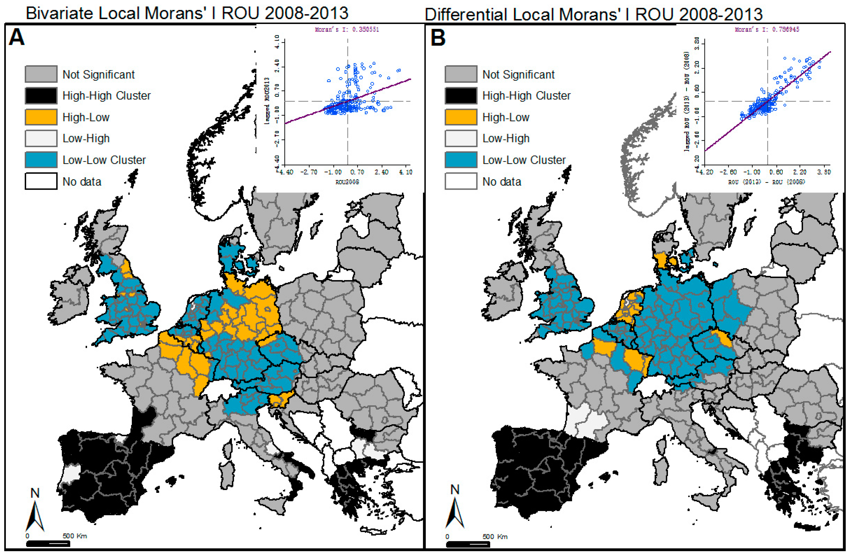
The map and scatter plot (Figure 5A) explain how the value of ROU in a location in 2008 affects the values of ROU in nearby locations in 2013. Results show local patterns of spatial correlation with Moran’s I = 0.35. High-high clusters are locations that, along with their neighbors, have high values of ROU in 2008 and are also surrounded by regions with high values in 2013. These areas can be considered as the result of the outward diffusion of ROU originating from the core in 2008 and spreading to the neighboring regions in 2013. In this respect, regions with high ROU in 2008 and also belonging to a high-high cluster, “infected” the surrounding areas in a kind of high ROU outbreak. Southern EU regions in Spain, Italy, and Greece belong to this group. Low-low clusters are areas that along with their neighbors have low values of ROU at both times. Similarly, low ROU values affected the nearby areas by reducing the ROU. These areas can be spotted in the U.K., north Italy and central Europe. Interesting findings are revealed in the high-low and low-high groups as well. The high-low group is located mainly in Germany, and partially in the U.K. and France. These regions, although exhibiting a high ROU in 2008, have a completely different status in 2013. Their ROU is now low, relative to the rest of neighboring regions for the same year. This does not necessarily mean the ROU in 2013 has decreased. The ROU might have increased and some regions still belong to this group, for example, regions in northern France (see Figure 1A,B) only because the rest of the regions have experienced significantly larger increases. The low-high ROU also reveals interesting patterns in regions that in 2008 had a low ROU but in 2013 are surrounded by high ROU regions. These regions can be found in Portugal, Italy, and Greece. These regions are among those that have been the most badly affected by the economic crisis. Not only did they significantly increase their ROU but they are also surrounded by regions with a high ROU, something that might lead to a slower recovery.
3.6. ROU Spatio-Temporal Autocorrelation 2008–2013: Differential Local Moran’s I
The differential Moran’s I map and related scatter plot are presented in Figure 5B. There is a strong positive spatio-temporal autocorrelation in the European regions with Moran’s I as high as 0.75. The local cluster map shows hot spots in Spain, Portugal, Greece, and Bulgaria, with larger changes in the ROU between 2008 and 2013. This typically means that the change over time of ROU in a given location is statistically related to the change of ROU among its neighbors. Cold spots are observed in the U.K., Germany, Austria, Belgium, and parts of Poland and France showcasing that changes were low over these five years. More analysis related to the above outcomes can be found in the discussion section.
4. Discussion and Conclusions
This paper distills the geographies of change of the ROU by applying advanced spatio-temporal autocorrelation techniques and procedures. A cross-regional spatio-temporal study covering the entire EU at the NUTS 2 regional level is carried out for two significant dates: the year 2008, which is regarded as the onset of the economic crisis, and the year 2013 where unemployment was at its peak. By selecting these two dates the study aims to adjust for the effect of the crisis in the ROU across Europe.
At the European level one out of four regions at least doubled its ROU in the period studied and another one out of four increased the ROU by 50–100%. The southern regions of Europe experienced large unemployment problems (Figure 1). Greece was severely affected by the crisis as all of its regions more than doubled their ROU during the study period. All Spanish regions at least doubled their ROU between 2008 and 2013 to at least 17.7%, which is larger than the maximum ROU for all European regions in 2008. At least a 15% ROU in 2013 was recorded in 80% of the regions in Spain, Greece, Portugal, and Italy. Germany was the only country that decreased the ROU in all regions during the crisis with the majority of regions showing a decrease of at least 20%. Only four other countries had one or two regions that experienced a slight decrease in ROU (on average around 10%). Of the regions with an ROU exceeding 15% in 2013, 87% are in Greece, Portugal, Spain, and Italy.
Global Moran’s provides us with a measure of spatial autocorrelation that allows for solid statistical analysis, in comparison to just mapping ROU and inspecting it visually. Although the general sense that ROU is clustered in specific areas can be grasped from Figure 1A,B, a statistical measure of this phenomenon is produced when using the spatial autocorrelation metrics. In this case study, global spatial autocorrelation was detected by applying Global Moran’s I for 2008 and 2013. Calculating Global Moran’s I at different times monitors how the metric changes. Results show (a) that spatial autocorrelation is more intense in 2013 revealing that the clustering of values is more evident in this year, and (b) that two different scales of analysis exist: in 2008, spatial autocorrelation is evident at 450 km while in 2013 spatial autocorrelation is evident at 750 km. This is a very interesting finding as it is a clear indication of an expanding process where the clustering of the ROU has been intensified between the two stamps. This intensification of clustering is the result of underlying processes, such as the economic crisis. This is also revealed when using the local indices of spatial autocorrelation.
From both local Moran’s I and Getis-Ord Gi* local spatial autocorrelation indices, results indicate that between 2008 and 2013, a high ROU is clustering in the southern European regions and is limited or decreasing in the central European regions. It is impressive that although there was a large cluster of high-high values (high ROU surrounded by high ROU) in 2008 in eastern Germany, in 2013 this cluster disappeared. At the same time, the rest of Germany’s regions are forming clusters of low-low values (Figure 4). It is probable that during the crisis many jobs were lost in the south and many jobs were created in central Europe and especially in Germany. In fact, Germany decreased the number of unemployed people by 836,000 while Greece, Spain, Portugal, and Italy added 6,181,000 new unemployed people (Table 1). This accounts for 65% of the total unemployed persons added within the study period in the EU.
From the spatio-temporal autocorrelation analysis it is apparent that the ROU is diffusing outwards and that there are different values patterns in south Europe compared to central Europe (Figure 5A). In this respect, high values are expanding to neighboring ones in the southern European regions and low values are expanding in central and Northern Europe. The central European regions are also exhibiting negative autocorrelation of a high-low pattern, which is more desirable in terms of decreasing the ROU.
The differential Moran’s I map clearly presents the geographical dimension of ROU evolution through the crisis period, and specifically locates the south as the most badly hit area with high rates of change in the ROU (Figure 5B). The positive spatial autocorrelation is so evident that the Moran’s I reaches a very high value of 0.75, which clearly identifies that changes over time in ROU are spatially clustered. The phenomenon of a high ROU was expanded throughout this five-year period in nearby areas like an outbreak. On the other hand, central European regions experienced low or even negative rates of change in the ROU.
This study provides a spatio-temporal analysis of the ROU for the EU26 regions and concludes that unemployment tends to cluster on a regional base. This conclusion is in line with other works highlighting that neighborhood effects are some times stronger than state effects in Europe [47]. In addition, the ROU is highly polarized and existing disparities across European regions before the crisis have been deepened further. This fact can be partially attributed to the strong socio-economic heterogeneities among the European regions. For example, southern European countries that where badly hit from crisis exhibited clusters of high unemployment rates in the pre-crisis period and where not well prepared in case of major recessionary shocks [48]. Most of these countries were characterized by overpriced housing market, huge construction sector, high export dependency and large public debts [49]. Eastern-European countries on the other hand, that joined the EU between 2004 and 2007 were still integrating their economy (at the period of crisis) into the common market with an ongoing trend of transition from agricultural to the service economy [15]. These transition countries were characterized by high dispersion of their human capital across regions and also high migration [50]. On the contrary, more resilient economies as those in central and northern Europe with better fiscal policies turned out to absorb smoothly the recessionary sock. The further widening of the gap between southern and northern European regions (illustrated by the large spatio-temporal autocorrelation increase) also unveils another interesting finding. The severe austerity measures imposed in the beginning of the crisis in many southern countries did not have any positive effect on unemployment mitigation. Plenty of regulations were imposed during 2010 and 2011 in these countries to control mainly national debt and climbing unemployment. For example, intensified labor flexibilization policies were harshly applied overnight in anticipation of economic growth and new jobs creation [7]. Although unemployment is not only affected by labor market regulations, results show that they had no positive effect on decreasing unemployment either. In fact, specific regions have been badly hit by high unemployment rates and are mentioned in detail above. As the ROU is an important indicator to assess the robustness and viability of an economy, the above results are in line with the poor economic conditions that Portugal, Spain, and Greece experienced in that period and also indicative of the sustainability of economies in central Europe [51,52,53,54].
From a broader policy perspective, results could be used from European governments to draw sub-national policies. The fact that spatio-temporal autocorrelation of ROU change is high reveals that policies with a cross-regional dimension should be applied at the local level to prevent the expansion of a high ROU. For example, locating the existence of spatial clustering and spatial autocorrelation in hot spot regions (high ROU) mainly located in southern-Europe can assist policymakers to design more efficient strategies that take into account spatial heterogeneity and thus apply local and tailored policies. As these regions have suffered from structural problems they require fiscal and industrial policies accompanied by related labor regulations that will create more resilient economies. Owing to the fact that regions that experience prolonged high unemployment rates are also prone to high economic inequality and low expected growth rates [9], it is advisable that planners and policy makers apply strategies that will alleviate problems in the population at hand. In this respect, governments should take measures with a local focus to strengthen the sectoral structure of regional economies and also narrow the gap with the more sustained ones. It is of high importance that national governments adopt policies that will increase their regional economic resilience for a potential future recessionary shock. The existence of spatial autocorrelation in unemployment suggests that quick and intense policy fixes through appropriate spatial planning should be applied when a high ROU exists in a period of crisis. These interventions should have a local focus to prevent the expansion of high ROU to neighboring areas; thus, controlling better the social and economic implications that unemployment brings.
Concluding, the present empirical analysis addresses the sub-national impact of economic crisis to ROU and identifies its spatio-temporal patterns. These findings can support a more advanced spatial planning approach for achieving society’s sustainability. Such analysis can be also integrated to econometric modelling to better identify the contextual factors behind regional unemployment and is planned for future research.
Funding
This research was funded by Sun Yat-sen University Starting Research Grant for George Grekousis, grant number [37000-18821113].
Conflicts of Interest
The author declares no conflict of interest. The founding sponsors had no role in the design of the study; in the collection, analyses, or interpretation of data; in the writing of the manuscript, and in the decision to publish the results.
References
- Torres, R.; International Labour Organisation; International Institute for Labour Studies. World of Work Report 2011: Making Markets Work for Jobs; ILO: Geneva, Switzerland, 2011. [Google Scholar]
- Eurostat European Commission. Regions in the European Union. Nomenclature of Territorial Units for Statistics; NUTS 2013/EU-28; Publication Office of the European Union: Luxembourg, 2013; Available online: http://ec.europa.eu/eurostat/documents/3859598/6948381/KS-GQ-14-006-EN-N.pdf (accessed on 10 January 2018).
- Brand, J.E.; Burgard, S.A. Job displacement and social participation over the lifecourse: Findings for a cohort of joiners. Soc. Forces 2008, 87, 211–242. [Google Scholar] [CrossRef] [PubMed]
- Gregg, P.; Tominey, E. The wage scar from male youth unemployment. Labour Econ. 2005, 12, 487–509. [Google Scholar] [CrossRef]
- Dieckhoff, M.; Gash, V. Unemployed and alone? Unemployment and social participation in Europe. Int. J. Sociol. Soc. Policy 2015, 35, 67–90. [Google Scholar] [CrossRef]
- Buffel, V.; Van de Velde, S.; Bracke, P. The mental health consequences of the economic crisis in Europe among the employed, the unemployed, and the non-employed. Soc. Sci. Res. 2015, 54, 263–288. [Google Scholar] [CrossRef] [PubMed] [Green Version]
- Gialis, S.; Taylor, M. A regional account of flexibilization across the EU: The ‘flexible contractual arrangements’ composite index and the impact of recession. Soc. Indic. Res. 2016, 128, 1121–1146. [Google Scholar] [CrossRef]
- Castells-Quintana, D.; Royuela, V. Unemployment and long-run economic growth: The role of income inequality and urbanisation. Investig. Reg. 2012, 24, 153–173. [Google Scholar]
- Stiglitz, J. The global crisis, social protection and jobs. Int. Labour Rev. 2013, 152, 93–106. [Google Scholar] [CrossRef]
- Brescia, R.H. The cost of inequality: Social distance, predatory conduct, and the financial crisis. N. Y. Univ. Annu. Surv. Am. Law 2010, 66, 641. [Google Scholar]
- Cracolici, M.; Cuffaro, M.; Nijkamp, P. A spatial analysis on Italian unemployment differences. Stat. Methods Appl. 2009, 18, 275–291. [Google Scholar] [CrossRef] [Green Version]
- López-Bazo, E.; del Barrio, T.; Artis, M. Geographical distribution of unemployment in Spain. Reg. Stud. 2005, 39, 305–318. [Google Scholar] [CrossRef]
- Vega, S.H.; Elhorst, J.P. A regional unemployment model simultaneously accounting for serial dynamics, spatial dependence and common factors. Reg. Sci. Urban Econ. 2016, 60, 85–95. [Google Scholar] [CrossRef]
- Pesaran, M.H. Estimation and inference in large heterogeneous panels with a multifactor error structure. Econometrica 2006, 74, 967–1012. [Google Scholar] [CrossRef]
- Marelli, E.; Patuelli, R.; Signorelli, M. Regional unemployment in the EU before and after the global crisis. Post-Communist Econ. 2012, 24, 155–175. [Google Scholar] [CrossRef]
- Signorelli, M. Employment and unemployment in a multilevel regional perspective. In L’Europe Me’Diterrane’Enne—Mediterranean Europe; Petricioli, M., Ed.; P.I.E. Peter Lang: Bruxelles, Belgium, 2008; pp. 175–200. [Google Scholar]
- Patuelli, R.; Schanne, N.; Griffith, D.A.; Nijkamp, P. Persistence of regional unemployment: Application of a spatial filtering approach to local labor markets in Germany. J. Reg. Sci. 2012, 52, 300–323. [Google Scholar] [CrossRef]
- Bailey, N.; Holly, S.; Pesaran, M.H. A Two-Stage Approach to Spatio-Temporal Analysis with Strong and Weak Cross-Sectional Dependence. J. Appl. Econ. 2016, 31, 249–280. [Google Scholar] [CrossRef]
- Chudik, A.; Pesaran, M.H.; Tosetti, E. Weak and strong cross-section dependence and estimation of large panels. Econ. J. 2011, 14, C45–C90. [Google Scholar] [CrossRef]
- Nijkamp, P. Regional development as self-organized converging growth. In Spatial Disparities and Development Policy; The World Bank Group: Washington, DC, USA, 2009; pp. 265–282. [Google Scholar]
- Oud, J.H.; Folmer, H.; Patuelli, R.; Nijkamp, P. Continuous-time modeling with spatial dependence. Geogr. Anal. 2012, 44, 29–46. [Google Scholar] [CrossRef]
- Andersson, D.E.; Andersson, Å.E.; Hårsman, B.; Daghbashyan, Z. Unemployment in European regions: Structural problems versus the Eurozone hypothesis. J. Econ. Geogr. 2015, 15, 883–905. [Google Scholar] [CrossRef]
- Doran, J.; Fingleton, B. Employment resilience in Europe and the 2008 economic crisis: Insights from micro-level data. Reg. Stud. 2016, 50, 644–656. [Google Scholar] [CrossRef]
- Patacchini, E.; Zenou, Y. Spatial dependence in local unemployment rates. J. Econ. Geogr. 2007, 7, 169–191. [Google Scholar] [CrossRef]
- LeSage, J.P.; Pace, R.K. Introduction to Spatial Econometrics; Taylor and Francis: Boca Raton, FL, USA, 2009. [Google Scholar]
- Gilmartin, M.; Korobilis, D. On regional unemployment: An empirical examination of the determinants of geographical differentials in the UK. Scott. J. Political Econ. 2012, 59, 179–195. [Google Scholar] [CrossRef]
- Rafferty, A.; Rees, J.; Sensier, M.; Harding, A. Growth and recession: Underemployment and the labour market in the North of England. Appl. Spat. Anal. Policy 2013, 6, 143–163. [Google Scholar] [CrossRef]
- Schwarz, P. Neighborhood effects of high unemployment rates: Welfare implications among different social groups. J. Socio-Econ. 2012, 41, 180–188. [Google Scholar] [CrossRef]
- López-Bazo, E.; Motellón, E. The regional distribution of unemployment: What do micro-data tell us? Pap. Reg. Sci. 2013, 92, 383–405. [Google Scholar] [CrossRef]
- Beyer, R.C.; Stemmer, M.A. Polarization or convergence? An analysis of regional unemployment disparities in Europe over time. Econ. Model. 2016, 55, 373–381. [Google Scholar] [CrossRef]
- Netrdová, P.; Nosek, V. Spatial patterns of unemployment in Central Europe: Emerging development axes beyond the Blue Banana. J. Maps 2016, 12, 701–706. [Google Scholar] [CrossRef]
- Blažek, J.; Netrdová, P. Regional unemployment impacts of the global financial crisis in the new member states of the EU in Central and Eastern Europe. Eur. Urban Reg. Stud. 2012, 19, 42–61. [Google Scholar] [CrossRef]
- Grekousis, G.; Mountrakis, G. Sustainable development under population pressure: Lessons from developed land consumption in the conterminous US. PLoS ONE 2015. [Google Scholar] [CrossRef] [PubMed]
- GISCO. Geographical Information and Maps. 2015. Available online: http://ec.europa.eu/eurostat/web/gisco/geodata/reference-data/administrative-units-statistical-units/nuts#nuts13 (accessed on 10 January 2017).
- Lloyd, C.D. Local Models for Spatial Analysis; CRC Press: Boca Raton, FL, USA, 2010. [Google Scholar]
- Rey, S.J. Space–Time Patterns of Rank Concordance: Local Indicators of Mobility Association with Application to Spatial Income Inequality Dynamics. Ann. Am. Assoc. Geogr. 2016, 106, 788–803. [Google Scholar] [CrossRef]
- Anselin, L. A Local Indicator of Multivariate Spatial Association: Extending Geary’s C. Center for Spatial Data Science, University of Chicago. 2017. Available online: https://s3.amazonaws.com/geoda/docs/LA_multivariateGeary1.pdf (accessed on 8 January 2018).
- Yamada, I.; Thill, J.C. Local indicators of network-constrained clusters in spatial point patterns. Geogr. Anal. 2007, 39, 268–292. [Google Scholar] [CrossRef]
- Anselin, L. Local indicators of spatial association—LISA. Geogr. Anal. 1995, 27, 93–115. [Google Scholar] [CrossRef]
- Getis, A.; Ord, J.K. The analysis of spatial association by use of distance statistics. Geogr. Anal. 1992, 24, 189–206. [Google Scholar] [CrossRef]
- Benjamini, Y.; Hochberg, Y. Controlling the false discovery rate: A practical and powerful approach to multiple testing. J. R. Stat. Soc. Ser. B Methodol. 1995, 57, 289–300. [Google Scholar]
- Benjamini, Y. Discovering the false discovery rate. J. R. Stat. Soc. Ser. B Stat. Methodol. 2010, 72, 405–416. [Google Scholar] [CrossRef]
- Caldas de Castro, M.; Singer, B.H. Controlling the false discovery rate: A new application to account for multiple and dependent tests in local statistics of spatial association. Geogr. Anal. 2006, 38, 180–208. [Google Scholar] [CrossRef]
- Goovaerts, P. How do multiple testing correction and spatial autocorrelation affect areal boundary analysis? Spat. Spatio-Temporal Epidemiol. 2010, 1, 219–229. [Google Scholar] [CrossRef] [PubMed]
- O’Sullivan, D.; Unwin, D. Geographic Information Analysis, 2nd ed.; Wiley: Hoboken, NJ, USA, 2010. [Google Scholar]
- Anselin, L. Exploring spatial data with GeoDaTM: A workbook. Urbana 2004, 51, 309. [Google Scholar]
- Garcilazo, J.E.; Spiezia, V. Regional Unemployment Clusters: Neighborhood and State Effects in Europe and North America. Rev. Reg. Stud. 2007, 37, 282–302. [Google Scholar]
- Hadjimichalis, C. Uneven geographical development and socio-spatial justice and solidarity: European regions after the 2009 financial crisis. Eur. Urban Reg. Stud. 2011, 18, 254–274. [Google Scholar] [CrossRef]
- Davies, S. Regional resilience in the 2008–2010 downturn: Comparative evidence from European countries. Cambr. J. Reg. Econ. Soc. 2011, 4, 369–382. [Google Scholar] [CrossRef]
- Jurajda, Š.; Terrell, K. Regional Unemployment and Human Capital in Transition Economies. Econ. Transit. 2009, 17, 241–274. [Google Scholar] [CrossRef]
- Antelo, M.; Magdalena, P.; Reboredo, J.C. Economic crisis and the unemployment effect on household food expenditure: The case of Spain. Food Policy 2017, 69, 11–24. [Google Scholar] [CrossRef]
- Anthopoulou, T.; Kaberis, N.; Petrou, M. Aspects and experiences of crisis in rural Greece. Narratives of rural resilience. J. Rural Stud. 2017, 52, 1–11. [Google Scholar] [CrossRef]
- Hudson, R. Facing forwards, looking backwards: Coming to terms with continuing uneven development in Europe. Eur. Urban Reg. Stud. 2017, 24, 138–141. [Google Scholar] [CrossRef]
- Starace, F.; Mungai, F.; Sarti, E.; Addabbo, T. Self-reported unemployment status and recession: An analysis on the Italian population with and without mental health problems. PLoS ONE 2017, 12, e0174135. [Google Scholar] [CrossRef] [PubMed]
Figure 1.
(A) ROU in 2008; (B) ROU in 2013; (C) Positive and negative change in ROU between 2008 and 2013; (D) ROU rate of change (%) between 2008 and 2013.
Figure 1.
(A) ROU in 2008; (B) ROU in 2013; (C) Positive and negative change in ROU between 2008 and 2013; (D) ROU rate of change (%) between 2008 and 2013.
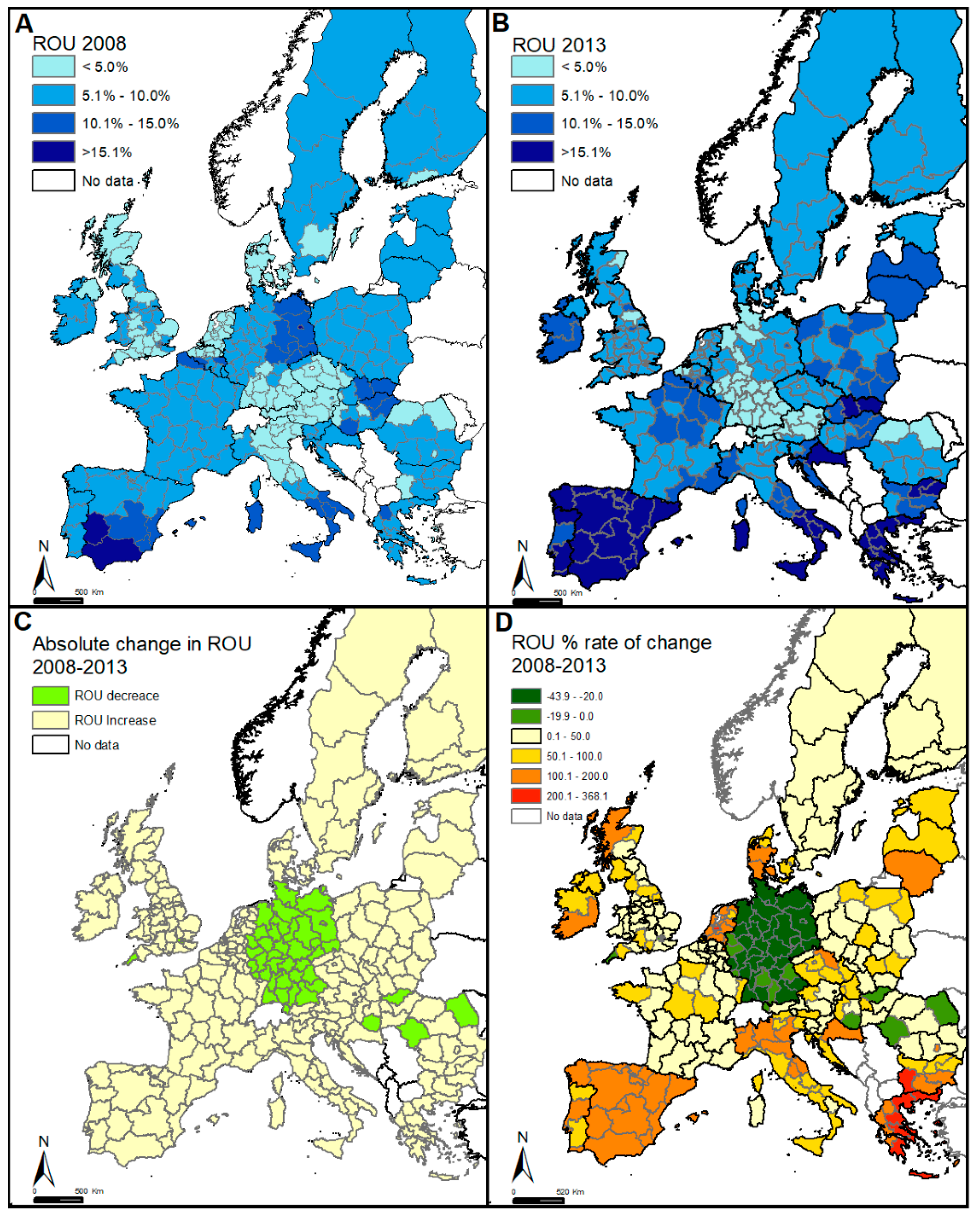
Figure 2.
Incremental spatial autocorrelation for ROU2008. All z-scores are statistically significant at less than 0.001 significance level.
Figure 2.
Incremental spatial autocorrelation for ROU2008. All z-scores are statistically significant at less than 0.001 significance level.
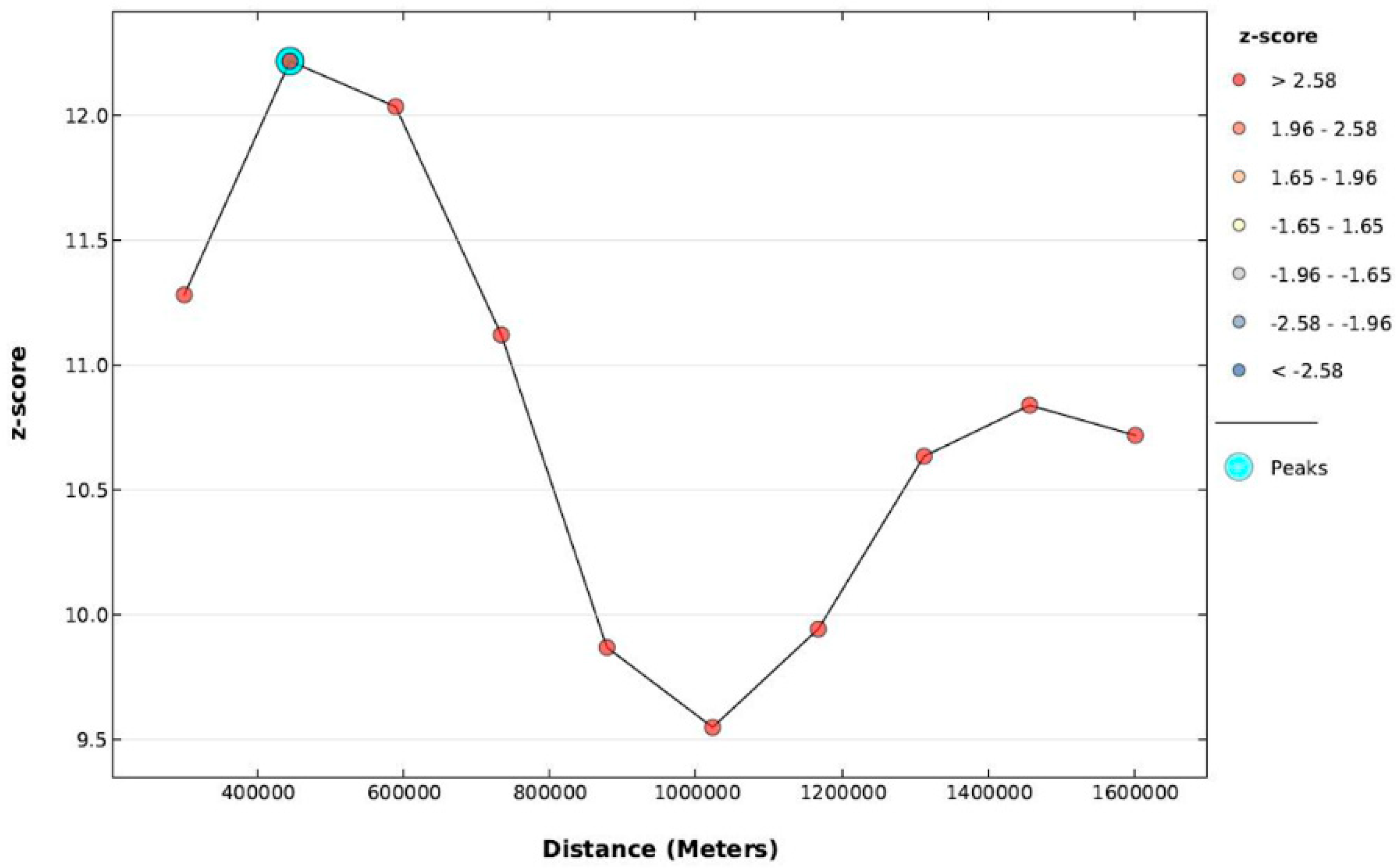
Figure 3.
Incremental spatial autocorrelation for ROU2013. All z-scores are statistically significant at less than 0.001 significance level.
Figure 3.
Incremental spatial autocorrelation for ROU2013. All z-scores are statistically significant at less than 0.001 significance level.
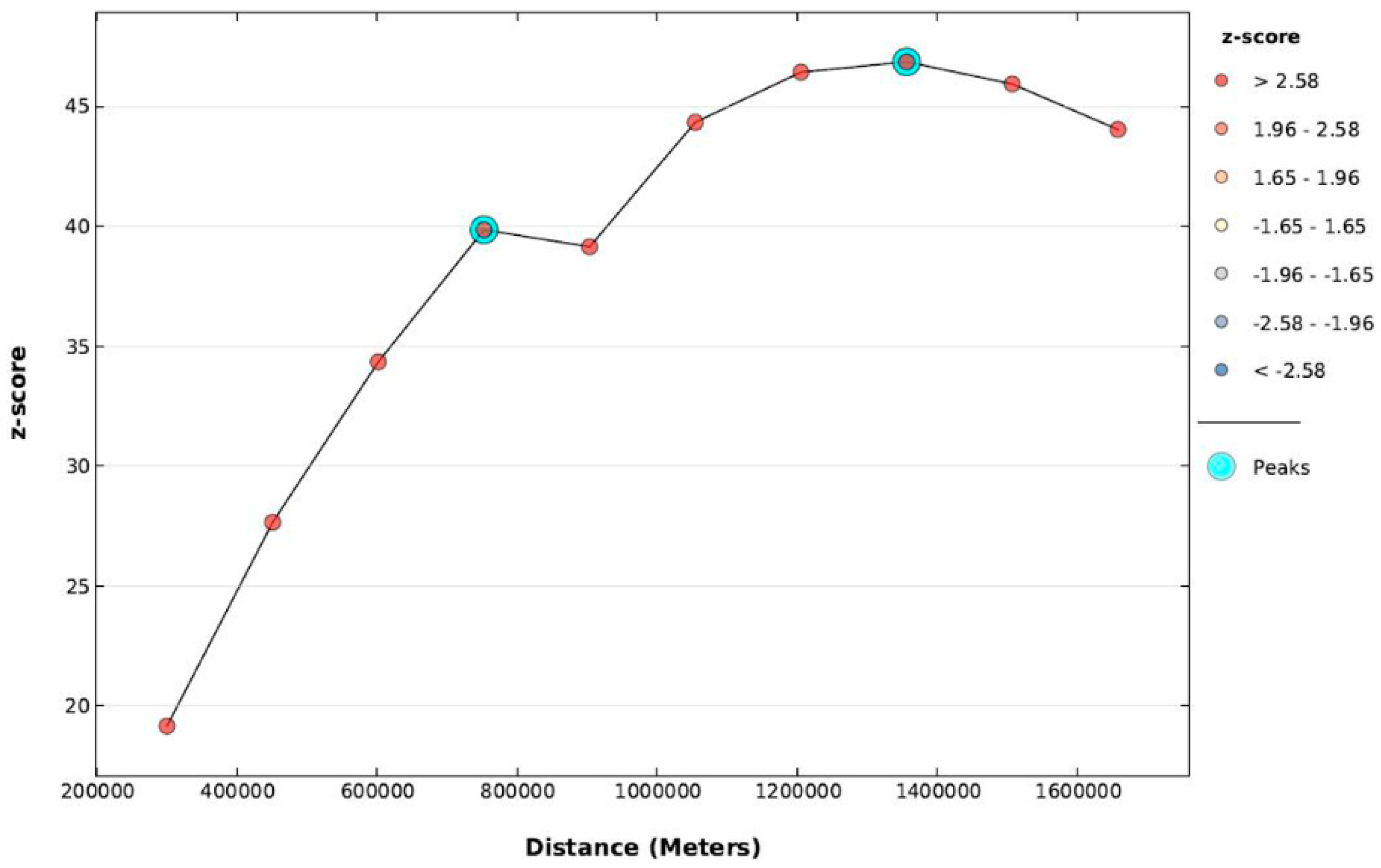
Figure 4.
Local spatial autocorrelation indices. (A) Local Morans’ I for 2008; (B) Local Morans’ I for 2013; (C) Getis-Ord Gi* for 2008; (D) Getis-Ord Gi* for 2013.
Figure 4.
Local spatial autocorrelation indices. (A) Local Morans’ I for 2008; (B) Local Morans’ I for 2013; (C) Getis-Ord Gi* for 2008; (D) Getis-Ord Gi* for 2013.
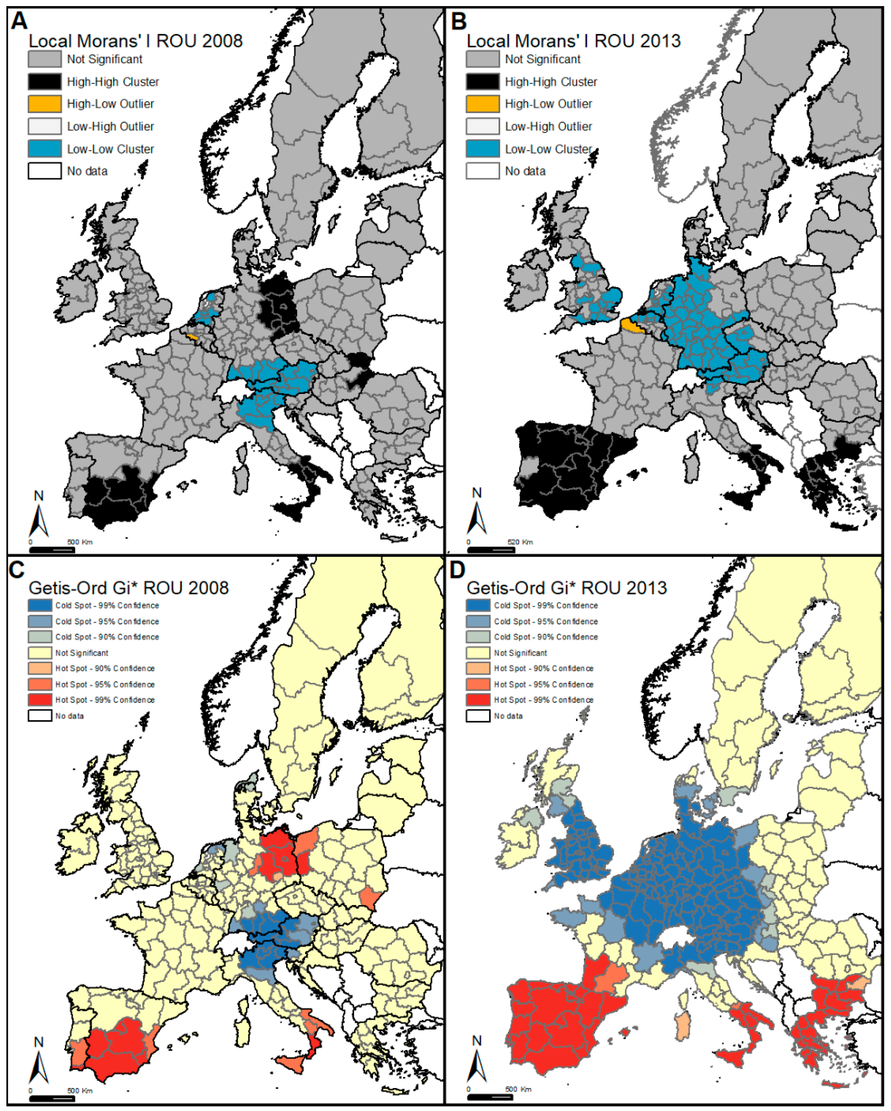
Figure 5.
(A) Bivariate Local Moran’s I for 2008–2013; (B) Differential local Moran’s I for 2008–2013. Moran’s I scatter plots are also embedded in the upper right corners of the maps.
Figure 5.
(A) Bivariate Local Moran’s I for 2008–2013; (B) Differential local Moran’s I for 2008–2013. Moran’s I scatter plots are also embedded in the upper right corners of the maps.


Table 1.
Country name, NUTS0 id per country, number of NUTS2 regions per country used in this study, unemployed people in thousands for 2008 and 2013, change of unemployment between 2008 and 2013, and per cent rate of unemployment for 2008 and 2013.
Table 1.
Country name, NUTS0 id per country, number of NUTS2 regions per country used in this study, unemployed people in thousands for 2008 and 2013, change of unemployment between 2008 and 2013, and per cent rate of unemployment for 2008 and 2013.
| Country | NUTS0 | NUTS2 Regions | Unemployment (in Thousands) | Change (in Thousands) | ROU (%) | ||
|---|---|---|---|---|---|---|---|
| 2008 | 2013 | 2013–2008 | 2008 | 2013 | |||
| Austria | AT | 9 | 172 | 231 | 59 | 4.1 | 5.4 |
| Belgium | BE | 11 | 333 | 417 | 84 | 7 | 8.4 |
| Bulgaria | BG | 6 | 202 | 436 | 234 | 5.6 | 13 |
| Czech Republic | CZ | 8 | 230 | 370 | 140 | 4.4 | 7 |
| Croatia | HR | 2 | 166 | 320 | 154 | 8.6 | 17.4 |
| Denmark | DK | 5 | 101 | 202 | 101 | 3.4 | 7 |
| Estonia | EE | 1 | 38 | 59 | 21 | 5.5 | 8.6 |
| Finland | FI | 5 | 172 | 219 | 47 | 6.4 | 8.2 |
| France | FR | 22 | 2121 | 3026 | 905 | 7.4 | 10.3 |
| Germany | DE | 38 | 3018 | 2182 | -836 | 7.4 | 5.2 |
| Greece | EL | 13 | 388 | 1330 | 942 | 7.8 | 27.5 |
| Hungary | HU | 7 | 326 | 441 | 115 | 7.8 | 10.2 |
| Ireland | IE | 2 | 146 | 282 | 136 | 6.4 | 13.1 |
| Italy | IT | 21 | 1664 | 3069 | 1405 | 6.7 | 12.1 |
| Latvia | LV | 1 | 88 | 120 | 32 | 7.7 | 11.9 |
| Lithuania | LT | 1 | 88 | 172 | 84 | 5.8 | 11.8 |
| Luxembourg | LU | 1 | 10 | 15 | 5 | 4.9 | 5.9 |
| Netherlands | NL | 12 | 318 | 647 | 329 | 3.7 | 7.3 |
| Poland | PL | 16 | 1165 | 1793 | 628 | 7.1 | 10.3 |
| Portugal | PT | 5 | 476 | 855 | 379 | 8.8 | 16.4 |
| Romania | RO | 8 | 549 | 653 | 104 | 5.6 | 7.1 |
| Slovenia | SI | 2 | 46 | 102 | 56 | 4.4 | 10.1 |
| Slovakia | SK | 4 | 254 | 386 | 132 | 9.6 | 14.2 |
| Spain | ES | 17 | 2596 | 6051 | 3455 | 11.3 | 26.1 |
| Sweden | SE | 8 | 305 | 411 | 106 | 6.2 | 8 |
| UK | UK | 40 | 1757 | 2437 | 680 | 5.6 | 7.5 |
| EU26 (study) | 265 | 16,729 | 26,226 | 9497 | |||
| EU28 | 276 | 16,751 | 26,304 | 9553 | 7 | 10.9 | |
© 2018 by the author. Licensee MDPI, Basel, Switzerland. This article is an open access article distributed under the terms and conditions of the Creative Commons Attribution (CC BY) license (http://creativecommons.org/licenses/by/4.0/).
Share and Cite
MDPI and ACS Style
Grekousis, G. Further Widening or Bridging the Gap? A Cross-Regional Study of Unemployment across the EU Amid Economic Crisis. Sustainability 2018, 10, 1702. https://doi.org/10.3390/su10061702
AMA Style
Grekousis G. Further Widening or Bridging the Gap? A Cross-Regional Study of Unemployment across the EU Amid Economic Crisis. Sustainability. 2018; 10(6):1702. https://doi.org/10.3390/su10061702
Chicago/Turabian StyleGrekousis, George. 2018. "Further Widening or Bridging the Gap? A Cross-Regional Study of Unemployment across the EU Amid Economic Crisis" Sustainability 10, no. 6: 1702. https://doi.org/10.3390/su10061702
Note that from the first issue of 2016, this journal uses article numbers instead of page numbers. See further details here.