A Multi-Stage Intelligent Model for Electricity Price Prediction Based on the Beveridge–Nelson Disintegration Approach

1
School of Economics and Management, North China Electric Power University, Beijing 102206, China
2
Beijing Key Laboratory of New Energy and Low-Carbon Development, North China Electric Power University, Changping, Beijing 102206, China
*
Author to whom correspondence should be addressed.
Sustainability 2018, 10(5), 1568; https://doi.org/10.3390/su10051568
Submission received: 22 April 2018
/
Revised: 10 May 2018
/
Accepted: 11 May 2018
/
Published: 14 May 2018
Abstract
:Accurate electricity price prediction is key to the orderly operation of the electricity market. However, the uncertain, stochastic and fluctuant characteristics of electricity pricees make prediction difficult. With the aim of solving this issue, this investigation proposed a multi-stage intelligent model integrating the Beveridge–Nelson decomposition (B-N-D) model, the least square support vector machine (LSSVM), and a nature-inspired optimization model named the whale optimization algorithm (WOA). Firstly, the B-N-D model was utilized to decompose the hourly electricity price time series into determinacy component, periodic trend, and stochastic item. Secondly, the WOA–LSSVM model was proposed to forecast the future hourly data of three components respectively, of which the optimal parameters of LSSVM were determined by using WOA. Finally, the future hourly electricity price data were computed by multiplying the forecasted data of those terms. To verify the validity of the proposed electricity price prediction model in this paper, five comparison approaches based on the B-N-D approach were selected, which are auto-regressive integrated moving average (ARIMA), single LSSVM, LSSVM optimized by the fruit-fly optimization algorithm (FOA), LSSVM optimized by particle swarm optimization (PSO) models, and WOA–LSSVM without B-N-D. By comparatively analyzing the error criteria values of the above models through testing on the objective data of the Pennsylvania–New Jersey–Maryland (PJM) electricity market collected from 11 December 2017 to 18 December 2017, from 15 January 2018 to 22 January 2018, and from 1 February 2018 to 25 February 2018, we conclude that the constructed intelligent model in this paper can greatly enhance the prediction precision of electricity prices.
1. Introduction
As the core of electricity market operations, accurate electricity price forecasting can help market participators to formulate reasonable competitive strategies and achieve risk minimization as well as benefit maximization [1]. For power-generation enterprises, according to accurate electricity price prediction decision makers need to assign an appropriate proportion of electricity to participate in day-ahead market transactions, real-time market transactions, auxiliary services market transactions, and bilateral contract transactions. Moreover, they also need to formulate corresponding bidding tactics to obtain maximum return and minimum risks [2]. For power-supply enterprises and other electricity buyers, based on precise electricity price prediction, they can optimally assign electricity purchasing amounts in the spot market. For electricity regulators, they need to monitor the power market in accordance with accurate electricity price forecasting to assure the stable and ordered development of the power market. Considering various factors affecting electricity prices as well as the uncertain and fluctuant nature of electricity prices, accurate price prediction is becoming an increasingly complicated problem [3].
The critical role of accurate electricity price prediction for electricity market participants has promoted the appearance of literature on forecasting electricity prices. The techniques used to forecast prices can be divided into two types, which are classical forecasting technologies and intelligent forecasting technologies [4]. The classical forecasting technologies are made up of some commonly used methods, including auto-regressive integrated moving average (ARIMA) [5], the dynamic regression (DR) method [6], as well as the generalized auto-regressive conditional heteroskedastic (GARCH) approach [7]. The intelligent forecasting technologies employ data-driven methods learning from historical data, containing artificial neural network (ANN) [8], support vector regression (SVR) based on ARIMA [9], and fuzzy neural network (FNN) [10] methods.
Moreover, in view of the nonlinear, fluctuting and inherent uncertaintainty of electricity prices and the complexity of predicting them, a series of hybrid methods has been proposed integrating classical and intelligent prediction techniques, which include the hybrid models combining mutual information (MI), wavelet transform (WT), and FNN on the basis of evolutionary particle swarm optimization (PSO) [11], MI-WT-SVM (support vector machine) on the basis of the gravitational search algorithm (GSA) [12], the integrated intelligent approach [13], and WT-ARIMA [14]. Among the literature on electricity price forecasting, it has been found that the ARIMA approach is one of the most widely used methods owing to its statistical advantages [4]. Additionally, Dong et al. [15] proposed an optimized prediction algorithm separating high fluctuation and daily electricity prices in Australia and employing empirical pattern disintegration method, seasonal arrangement and the ARIMA approach. Mandal et al. [16] put forward an integrated intelligent method combining a data-screening method according to the WT approach, an optimization algorithm on the basis of the firefly model, and a soft calculating technique using a fuzzy art-map (FA) network to predict day-ahead power priced for the Ontario electricity market. Wu et al. [17] established a recursive dynamic factor analysis (RDFA) model using an effective subspace tracing approach to track critical components and a Kalman filter approach to trace and predict critical components scores. In [18], a three-tier front feed neural network model was proposed to predict electricity prices for next-week in the power markets of Spain and California. Abedinia et al. [19] presented a prediction engine based on a combinatorial neural network (CNN) integrating with a new training method on the basis of a revised chemical reaction optimization method to select optimal weights of CNN for forecasting electricity price data.
Based on the existing research literature in the field of electricity price forecasting, developing more precise prediction approaches for power price is required due to the complex electricity market environment and requirement for electricity price forecasting accuracy. This investigation concentrates on next-day hourly electricity price forecasting that is an electricity price prediction procedure commonly employed by participants in the power market for preparing their bids. The novel dedications of this paper are listed as below:
- (1)
- An integrated multi-stage intelligent electricity price forecasting model is proposed combining the Beveridge–Nelson decomposition (B-N-D) model, the least square support vector machine (LSSVM) method, as well as a nature-inspired intelligent optimization approach named the whale optimization algorithm (WOA).
- (2)
- In the stage of data processing, the B-N-D approach, for the first time to our knowledge, is used to decompose the original electricity price data series into deterministic component, stochastic item and cyclic trend, taking the fluctuant, random, and uncertain nature of power price data into consideration.
- (3)
- In the stage of forecasting, the disintegrated three components will be respectively predicted by employing the LSSVM model, the regularization parameter ‘c’ and the radial basis function (RBF) kernel width ‘σ’ which are optimally selected by the novel optimization method WOA.
The performance of the established integrated multi-stage intelligent electricity price forecasting model will be tested on the day-ahead power market of Pennsylvania–New Jersey–Maryland (PJM) in the United States of America. The forecasting superiority of the proposed model will be verified through comparing it with several models based on B-N-D approach, including single LSSVM, LSSVM optimized by PSO, LSSVM optimized by FOA and ARIMA, and LSSVM optimized by WOA, without disintegrating the initial electricity price data by B-N-D approach.
The other sections of this research are structured as below. Following the introductory section, the basic theories employed in this research are elaborated. Section 3 depicts the detailed course of the constructed multi-stage intelligent electricity price prediction model. Section 4 provides the prediction results of the established multi-stage intelligent model. Section 5 comparatively analyzes the prediction manifestation of the constructed model and another five selected comparison models. Section 6 obtains the conclusions.
2. Theoretical Framework for Electricity Price Forecasting
The established integrated multi-stage intelligent electricity price forecasting model contains the B-N-D approach, LSSVM method, and an intelligent optimization approach named WOA. This section will elaborate the basic theories of these three approaches.
2.1. Beveridge–Nelson Decomposition (B-N-D) Approach
In order to resolve the first order differential stable data series, Beveridge and Nelson presented the B-N-D approach by which the data series co-integrated at the first order can be disintegrated into transitory component and permanent trend. The permanent trend is composed of a determinacy component and random item. The temporary item has a stable course with zero average data, which is called the cyclic term [20,21,22,23].
Considering the disintegration qualifications of the B-N-D approach, it is required to demonstrate whether the data series are stable after the first differencing. If they are stable after first order differencing, then the B-N-D approach can be conducted as below.
Suppose the natural logarithmic values of hourly electricity prices to be in the first order stable form in terms of the Wold theorem:
where , Pt represents the power price in time point t, μ demonstrates the average value for in the long-run, εt~ (i.i.d. implies independently and identically distribute), t indicates time, and λi is the coefficient. The expectation data of the above equation can be written as:
where E is a function employed to calculate the expected data of every variable.
Since lnPt represents the natural logarithm data of power price, the first order difference of it means the growth ratio of the power price. Considering Equation (2), the average data of the growth ratio of the power price demonstrates the long-term growth rate. According to the B-N-D theory, the deterministic component DTt can be disintegrated as:
where DTt demonstrates the determinacy component at t time point, and represents the original logarithm data of the power price.
Moreover, lnPt is deemed as the forecasting data in accordance with current information. Morley [24] held the opinion that such time series can be predicted more precisely via use of a steady uni-variate auto regressive (AR) Equation (1) formula at first order, which can be depicted as:
where can be calculated through AR Equation (1) formula and . Based on the Wold form in the AR Equation (1) formula, according to the normality hypothesis, the minimum average squared error (MASE) of period j ahead forecasting of the first order of ΔlnPt can be written as:
In line with the decomposition identification of B-N-D [20], the total tendency item of time series represented by Tt is deemed to be the MASE forecasting from the long-run level. It is equal to the current level of the sequences and the infinite sum of the MASE of period j ahead of the first order prediction:
where Tt is defined as the total item of data series.
Integrating Equations (5) and (6), based on the infinite sum formula of isometric series (due to ), the total component of lnPt after being decomposed by B-N-D under the condition of AR(1) can be calculated by:
The cyclic item of lnPt can be calculated as:
where Ct illustrates the cyclic item at t time point.
The stochastic item can be computed according to Equations (3), (7), and (8), namely:
where STt indicates the random term at t time point.
2.2. Least Square Support Vector Machine (LSSVM) Model
The LSSVM is an improved algorithm of the support vector machine (SVM). Considering that the minimum structural risks by regularization restrict that have built up on the weights of the model, the LSSVM alleviates the problem of convex quadratic programming associated with SVM [25,26,27]. The merits of LSSVM contain setting slack via equality restricts and calculating the regression issues as a series of linear formulas bringing about rapid training as well as more precision and stability [28]. The basic theoretical framework of LSSVM is elaborated as below.
Set up samples series , and suppose as input variables and as output data of sample i. Through utilizing the function , the sample series are mapped into a higher dimensional space from the initial characteristic space, hence it can be written in a linear form:
where demonstrates the weights vector and b illustrates the deviation term.
In virginal space, the LSSVM approach with an equality restrict is depicted as:
where c demonstrates the regularization parameter and ξi implies the slack component.
The Lagrangian function L is adopted [29], and then the qualifications for Karush–Kuhn–Tucker (KKT) for optimality are identified by:
where ai implies Lagrange multiplier.
Eliminating the series w and , the optimization procedure is converted to the linear formula. To be consistent with Mercer’s requirements, the Kernel function is described as:
The LSSVM approach for regression is elaborated as:
Radial basis function (RBF) is selected as the Mercer Kernel function in this investigation due to the fewer parameters that need to be identified and the advantageous manifestation, which is illustrated as:
2.3. Whale Optimization Algorithm (WOA)
Prompted by the premium hunting behaviors of humpback whales [32], the scholar Seyedali Mirjalili established a nature-inspired optimization algorithm called WOA, which is employed to analog the distinctive behaviors of humpback whales [33]. The hunting behavior explored by Goldbogen et al. discovered that there exist two kinds of plots associated with bubbles, which are ‘upward-spirals’ and ‘double-loops’ [34]. In the former tactic, the whales dive down several meters and spit bubbles in a twist-form around the hunting objects and move to the surface excerpted from the previous study [33]. Hence, the mathematical simulation of the twist shape bubble-net hunting tactic is helpful for conducting optimization. The WOA is presented based on such behavior.
The WOA is composed of five steps based on the spiral bubble-net hunting tactic elaborated as:
● Step 1: Parameters installation
The critical parameters of WOA are the number of search individuals SearchAgents_no, the number of investigated variables dim, the maximum amount of iterations Max_iteration, the lower limit lb = [lb1, lb2, ….., lbn−1, lbn], and upper limit ub = [ub1, ub2, ….., ubn−1, ubn] of variables.
● Step 2: Population initialization
Since the WOA is an algorithm based on population, the positions of whales in WOA are set in a matrix as:
where W is the position matrix of various search individuals, illustrates the data of j-th parameter for i-th search individual, , . The parameter can be obtained through utilizing the random distribution written as the following equation:
where W(i, j) demonstrates the entry in the i-th row and j-th column in matrix W, lb(i) and ub(i) illustrate the bottom and upper limits for i-th search individual, rand(i,j) means the random data obtained from the uniform distribution ranging from 0 to 1.
● Step 3: Fitness function identification
During the optimization course, the fitness function f[*] needs to be identified to evaluate each search individual, and the fitness values of each search individual are stored in the matrix OW, which are depicted as below:
● Step 4: Iteration procedure
For WOA, the searching individuals regenerate their locations in terms of a randomly chosen searching individual or the best tactic discovered up to now. With the purpose of avoiding local optimum and achieving global exploration, the WOA starts searching with several stochastic tactics, which demonstrates the position of a search individual is renewed with respect to a randomly chosen search individual. The mathematical formula is shown as:
where demonstrates the stochastic place vector selected from present searching individuals, means the current position vector, and represent coefficient vectors, t is the generation, | implies calculating the absolute value, and · is the multiplying computing process. The vectors and are calculated as:
where linearly decreases from 2 to 0 in iteration procedure, and is a stochastic vector in the scope of 0–1.
Values of are decided by the diversification of and the random values of , and the absolute values of determine whether the process is exploration or exploitation. A stochastic individual is selected if , which implies an exploration process. While the best resolution is found if to regenerate the places of the searching individuals, which demonstrates the exploitation process. For , whales swim around the hunting objects in contractible circles and spiral paths.
For the contractible circle path, the searching individuals regenerate their places in accordance with the following formula:
where implies the place vector storing the best solution discovered up to now. The vector and can be obtained in terms of Equations (21) and (22). The contractible circle mechanism can be realized via decreasing the value of in Equation (21).
For the spiral shape track, it can be imitated as:
where is the distance of the whale to the hunting object (the best solution found up to now), b demonstrates a constant employed to identify the path of the logarithmic twist, and l represents random data generated from the interval [−1, 1].
Considering that the whales move around the optimum solution both in a contractible circle and twist shape path, to simulate such behavior, it is supposed that there exists 50% feasibility to choose the twist path or contractible circle path to regenerate the location of whales in searching optimum solution course. Such modeling process can be mathematically constructed as:
where p is a random data generated from 0 to 1. If p < 0.5, the whales move around the optimum solution in a contractible circle. While if , the whales move around the optimum solution in a twist shape path.
● Step 5: Optimum solution selection.
Through the iteration procedure, the searching individuals regenerate their locations in terms of a random searching individual that is found or the optimum tactic discovered up to now. A stochastic searching individual can be found if , and the searching individuals restores their place based on Equation (20). Otherwise, the optimum solution is selected if , and the searching individuals renew their locations based on Equations (24) and (25) determined by the value of p. Ultimately, if the iteration requirement is met, the iteration of WOA comes to an end.
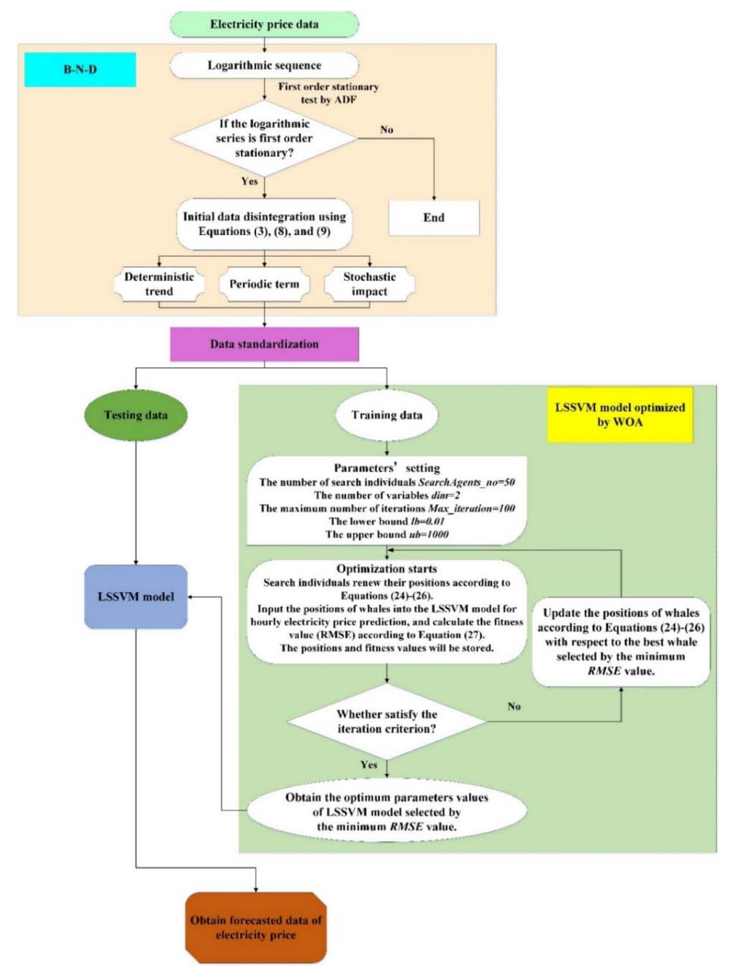
3. The Course of the Constructed Multi-Stage Intelligent Model for Electricity Price Prediction
In this study, an integrated intelligent algorithm is established to improve the precision of electricity price prediction. Considering the uncertain and fluctuant inherent nature of electricity price data and the interference of stochastic effects on power price data, the B-N-D approach is used to decompose the original hourly electricity price data into determinacy term, cyclic item, and random component. After that, the LSSVM method is applied to forecast three decomposed terms respectively. Finally, through multiplying the prediction results of these three data series, the forecasted electricity price data are obtained. Before forecasting by the LSSVM approach, the optimal values of two parameters ‘σ’ and ‘c’ related to the LSSVM approach need to be selected. This paper employs the latest nature-inspired optimization approach WOA to select the optimal values of those two parameters to enhance the forecasting precision.
The multi-stage forecasting procedures of the electricity price are elaborated as below.
● Step 1: First order stationary examination
In view of the fundamental principles of the B-N-D, it is essential to test whether the first difference form of logarithmic series of the original data is steady. The augmented Dickey–Fuller (ADF) methodology is applied to conduct the first order stability test. Only if the logarithmic form of the initial data is stable after first differencing, the next stage can be stepped.
● Step 2: Original data series disintegration
Since the logarithmic series of original data are stable at first order, the original data can be disintegrated into determinacy trend, cyclic item, and random impact effect in terms of Equations (3), (8) and (9).
● Step 3: Parameters’ setting
In WOA, several parameters need to be installed according to Section 2.3. Based on the examples in Ref. [33] and the research object of this paper, we suppose SearchAgents_no = 50, dim = 2, Max_iteration = 100, lb = 0.01, and ub = 1000.
● Step 4: Optimization beginning
By utilizing WOA for selecting the optimal values of LSSVM’s two parameters, it is required to determine the fitness function f[*] firstly. In this investigation, the root mean square error (RMSE) illustrated as below is employed as f[*].
where x(k) demonstrates the historical value of electricity price at time point k, and means the calculated value of electricity price at time point k.
The locations of searching individuals are utilized to indicate the parameters of the LSSVM approach, which are set as and . At the first generation, the fitness values of all searching individuals are calculated employing Equation (27). Then, the population of all searching individuals can be ranked in accordance with the fitness values, and the searching individuals with optimum fitness data are chosen according to the minimum values of RMSE. Since the best searching individual with the minimum RMSE value is discovered, other searching individuals will regenerate their locations related to the best one based on the Equation (26).
● Step 5: Optimization termination
After the first generation, the best searching individual and the optimum fitness value can be generated. Then, the offspring iteration can be conducted, and the searching individuals renew their positions according to the Equations (24)–(26) with respect to the best searching individual selected by the minimum values of RMSE. After 100 iterations, the minimum RMSEs can be discovered, and the optimum data of ‘σ’ and ‘c’ are found. After that, the optimized LSSVM is constructed, and the data of electricity prices are finally calculated and forecasted.
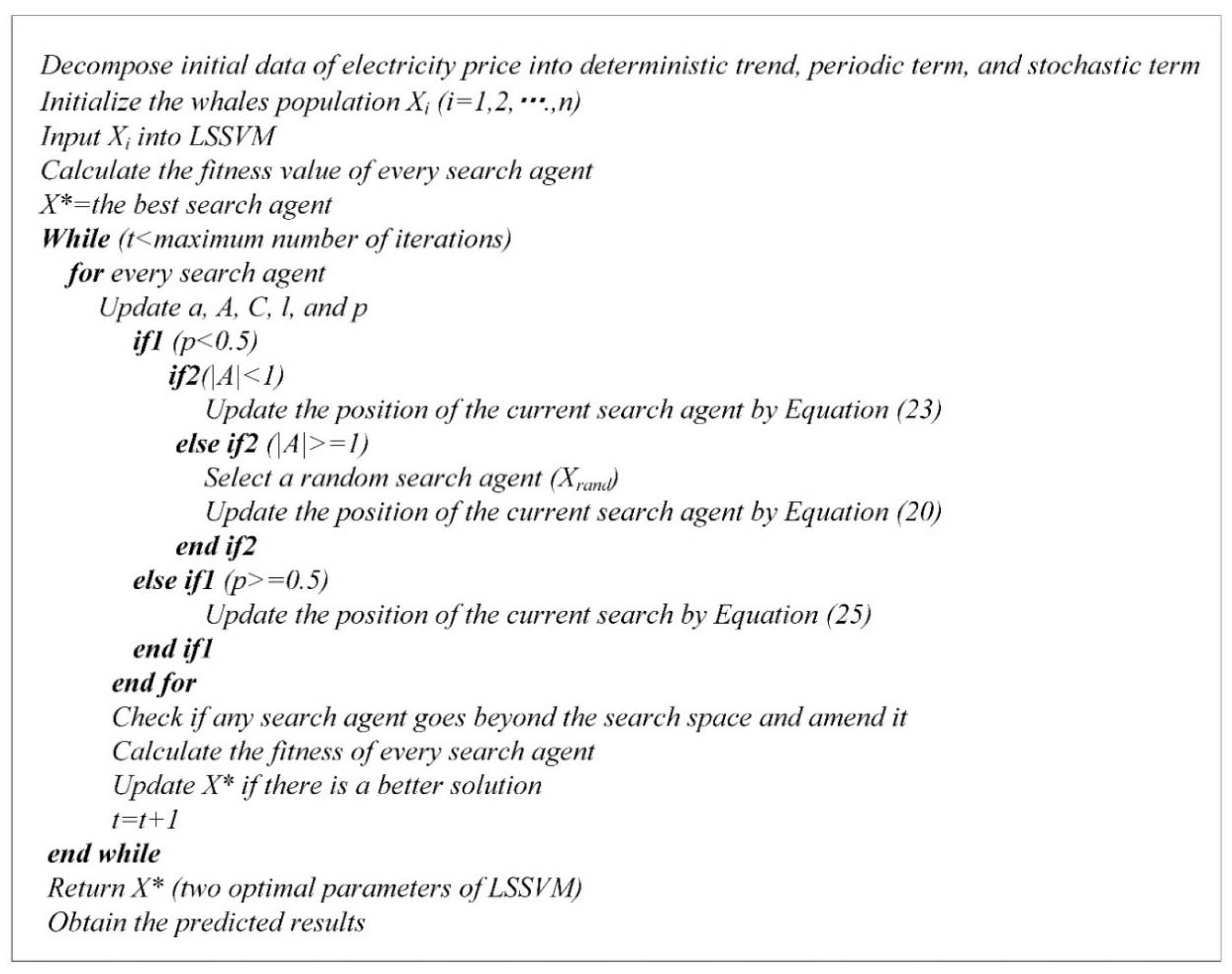
The course of the constructed multi-stage intelligent model of electricity price forecasting is demonstrated as Figure 1. The pseudo code of the proposed electricity price forecasting model is illustrated in Figure 2. Through conducting the pseudo code in Figure 2, we can obtain the optimal parameters of LSSVM and then we can forecast electricity price data via substituting the optimal parameters into LSSVM.
4. Empirical Analysis
4.1. B-N-D Results
The established multi-stage intelligent model for electricity price forecasting is employed to test real data of the PJM electricity markets [35]. Data on 192 h of electricity prices from 11 December 2017 to 18 December 2017 constitute the research dataset. Among them, the first 168 h of electricity price data are selected to be the training sample data, and the last 24 h electricity price data are treated as testing data to assess the forecasting precision for the established integrated model.
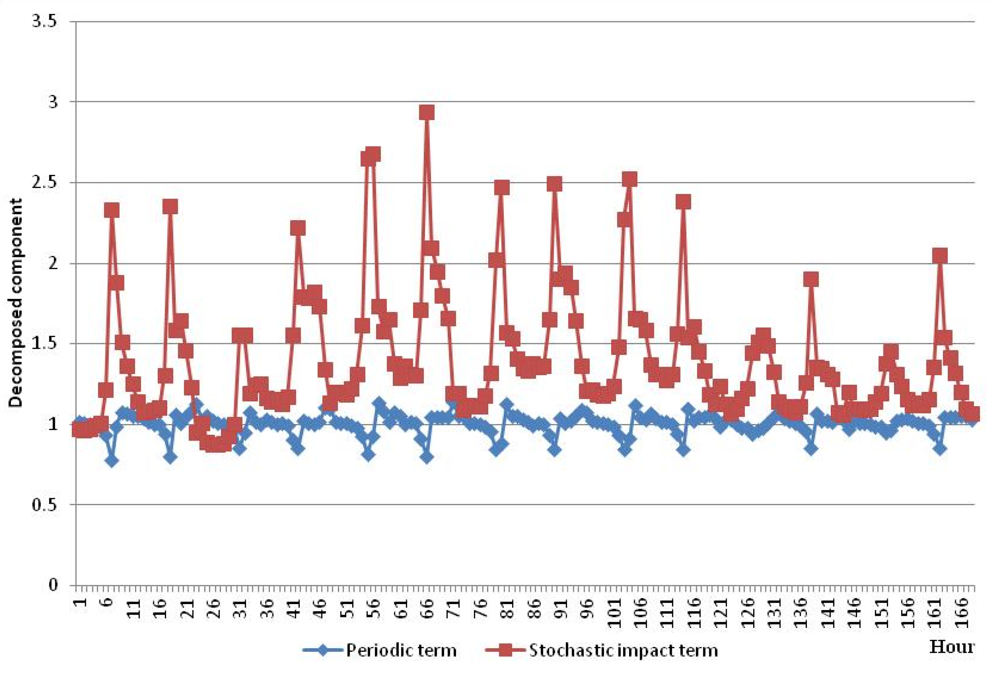
At the first stage, the B-N-D model is applied to decompose the logarithmic form of original 168 h electricity price data. Before disintegrating, considering the qualifications of the B-N-D approach, it is required to test whether the first order of the logarithmic form of original hourly electricity price data is stationary employing the ADF unit root examination method. As is shown in Table 1, the hourly electricity price data series are stationary at first order, and it can be known that the qualification of B-N-D is met whereby the data series can be co-integrated at first order. Therefore, we can disintegrate the logarithmic form of hourly power price data into the determinacy trend, cyclic item and random component through applying Equations (3), (8) and (9). Considering that the obtained three components are all in logarithmic form, we should convert them into natural form to be applied for the WOA-LSSVM method. The disintegrated results of those three components in natural form are shown in Figure 3 and Figure 4. The determinacy trend demonstrates the data series shows a decreasing tendency over the time changes. The stochastic impact effect illustrates the influences of unexpected and uncertainty stochastic factors on data series. The cyclic item implies the periodical change of electricity price data series.
4.2. WOA-LSSVM Prediction Results Based on B-N-D
After obtaining the natural forms of the deterministic trend, periodic term, and stochastic impact effect of hourly electricity price, the LSSVM optimized by WOA is utilized to respectively predict these three items, and the electricity price data can be predicted via multiplying the forecasted data of those terms. Considering the data availability, when those three components are forecasted by WOA-LSSVM, the data at the last moment and the data at the same moment of yesterday are treated as the input data series. Taking the determinacy trend as an example, when future data of the determinacy trend is forecasted, the determinacy trend data at the last moment and at the same moment of yesterday are fed into the WOA-LSSVM model.
Before employing the WOA-LSSVM method to predict those three components, the sample data should be standardized into the interval [0, 1] according to the following equation:
where xmin and xmax demonstrate the minimum and maximum values of training and testing data.
For the WOA-LSSVM method, two parameters ‘c’ and ‘σ’ in the LSSVM approach are optimally selected by the WOA. During iteration, the optimum data of ‘σ’ and ‘c’ in LSSVM for deterministic trend forecasting, stochastic component forecasting and periodic trend forecasting are selected according to the minimum values of RMSE. The optimal values of them are illustrated in Table 2.
During testing process, the determined values of ‘σ2 ‘and ‘c’ are utilized to compute the prediction values of the determinacy term, cyclic item and stochastic item of electricity price series, respectively. The predicted electricity price data are computed through multiplying the prediction data of those items. The prediction accuracy is evaluated by two error criteria, namely RMSE calculated by Equation (27) and mean absolute percentage error (MAPE) computed as Equation (29).
where demonstrates the historical data at k time point, and implies the predicted data at k time point.
The RMSE and MAPE of the established WOA-LSSVM method based on B-N-D for each hour are demonstrated in Table 3. It indicates that the values of MAPE and RMSE at the 21st hour are the smallest, which are respectively 0.02% and 0.006. The MAPE at the 23rd hour is the largest, which is 1.40%. The MAPE values at other hours are in the range of 0.03%–1.31%, and the RMSE values range from 0.007 to 0.381. The mean values of MAPE and RMSE are, respectively, 0.54% and 0.182, which are relatively small compared to the previous literature. Hence, it is known that the established multi-stage intelligent model can improve the prediction precision of electricity price effectively.
5. Prediction Performance Comparison
With the aim of comparing the prediction performances, five comparison prediction approaches are selected including ARIMA, single LSSVM, LSSVM optimized by fruit-fly optimization algorithm (FOA-LSSVM), and LSSVM optimized by particle swarm optimization (PSO-LSSVM) models based on B-N-D approach, as well as WOA-LSSVM based on the initial electricity price data without B-N-D, testing at three different periods the electricity price data collected from the PJM electricity markets. For the single LSSVM, PSO-LSSVM, and FOA-LSSVM models based on the B-N-D approach, the input data series and output data series are the same as the established WOA-LSSVM based on B-N-D approach, while the diversity among these models is that the mechanism of parameters’ determination. For the ARIMA method, when the deterministic term, periodic term and random item are predicted, only the historical data of component itself are used to predict the corresponding term without considering the data of the last moment and the data at the same moment of yesterday. For the WOA-LSSVM based on the initial electricity price data without the B-N-D, the initial electricity price data are employed to predict future data of hourly electricity price, for which the electricity price data at last moment and at the same moment of yesterday are taken as input data series.
Based on the electricity price data series mentioned in Section 4, for the single LSSVM approach based on B-N-D (B-N-D-LSSVM), the corresponding values of the determinacy trend, periodic item and stochastic effect at the last moment and at the same moment of yesterday from 1 to 168 h are treated as the input data series to predict three items respectively. Then, through learning the historical data, the optimized values of ‘σ2‘ and ‘c’ are found [36]. Finally, hourly electricity price data in the next 24 h can be predicted.
For the FOA-LSSVM model based on B-N-D (B-N-D-FOA-LSSVM), the parameters ‘σ2‘ and ‘c’ in LSSVM approach are used to respectively predict the deterministic trend, periodic item and stochastic effect, and are determined by FOA through optimization iteration. Similar to WOA, there are also several parameters that need to be initialized in FOA, which are the maximum iteration set as 100, and the amount of searching individuals supposed to be 50, (X_axis, Y_axis) ⊂ [−50, 50], FR ⊂ [−10, 10], X_axis = rands(1, 2), and Y_axis = rands(1, 2). Then, the optimal value of ‘σ2‘ and ‘c’ can be discovered, and future electricity price data can be forecast.
For the PSO-LSSVM method based on B-N-D (B-N-D-PSO-LSSVM), parameters ‘σ2‘ and ‘c’ in the LSSVM approach used to respectively predict determinacy trend, cyclic item and stochastic effect are selected by PSO through iteration. It is also necessary to initialize several parameters in PSO, including max_iteration = 100, swarm size = 30, particle size = 2, the minimum of the particle= [0.01, 100], the maximum of the particle= [0.1, 1000], the lower limit of velocity = −500, the upper limit of velocity = 500, and learning factors c1 = 1.5, c2 = 1.7. Then, the best values of ‘σ2‘ and ‘c’ can be explored by PSO, and the electricity price data can be forecast.
The ARIMA based on B-N-D (B-N-D-ARIMA) has been widely used in previous literature related to electricity price forecasting [4,9]. The ARIMA method can be utilized to forecast the non-stationary time series. It regards time series as a stochastic process which can be simulated and depicted by a mathematical model. After the mathematical model is identified, the future data can be predicted by the past and present time series data. This method takes the dynamic and persistent characteristics of time series into account, which can reveal the interaction between the past and present time series and between the present and the future time series. Considering the deterministic term, cyclic component and random trend, the ARIMA method is used to simulate the variation tendency of the past 168 h of these three components, and then the future 24 h of the corresponding terms will be forecast. Therefore, the future 24 h power price data can be forecast by multiplying the forecasted three components.
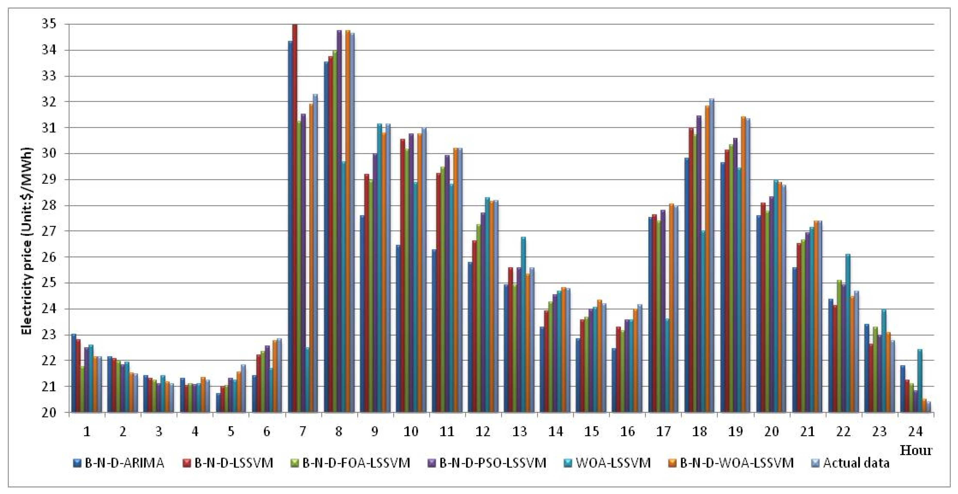
According to the principles of aforementioned models, the future 24 h electricity price data can be predicted. The parameters values of B-N-D-LSSVM, B-N-D-FOA-LSSVM, B-N-D-PSO-LSSVM, and WOA-LSSVM are illustrated in Table 4. The forecasting results of B-N-D-LSSVM, B-N-D-FOA-LSSVM, B-N-D-PSO-LSSVM, B-N-D-WOA-LSSVM, B-N-D-ARIMA and WOA-LSSVM are illustrated in Figure 5. It can clearly be seen that the gap between B-N-D-WOA-LSSVM and actual electricity price data is the smallest, followed by B-N-D-PSO-LSSVM. While the gap between WOA-LSSVM and actual electricity price data is the largest, followed by B-N-D-ARIMA.
To further analyze the forecasting performances of all models, MAPE and RMSE are applied according to Equations (27) and (29). The calculated data of MAPE and RMSE are demonstrated in Table 5. It can be seen that the MAPE and RMSE values of B-N-D-WOA-LSSVM are the smallest, respectively 0.54% and 0.18, while the MAPE values of B-N-D-PSO-LSSVM, B-N-D-FOA-LSSVM, and B-N-D-LSSVM are respectively 1.44%, 2.76%, and 3.07%. Therefore, it can be concluded that the optimization algorithm WOA can effectively select the optimal data of two parameters in LSSVM, which can greatly increase the prediction accuracy of LSSVM in electricity price forecasting. By comparing the MAPE and RMSE values of B-N-D-LSSVM and B-N-D-ARIMA, it can be found that the LSSVM method is more accurate than ARIMA method in electricity price forecasting. By comparatively analyzing the MAPE and RMSE of B-N-D-WOA-LSSVM and WOA-LSSVM, it is apparent that the B-N-D approach can significantly improve the forecasting accuracy by 5.23%. Since the B-N-D method can disintegrate the electricity price data into the determinacy trend, cyclic item and random effect, the uncertainty, stochastic, and fluctuation instincts of electricity price data can comprehensively be considered when these three components are forecast, and hence the forecasting precision can be improved greatly. By comparing the B-N-D-WOA-LSSVM with B-N-D-PSO-LSSVM, B-N-D-FOA-LSSVM, B-N-D-LSSVM, B-N-D-ARIMA and WOA-LSSVM, it is confirmed that the proposed multi-stage intelligent model employing LSSVM optimized by WOA based on the B-N-D approach can effectively enhance the prediction precision of electricity prices.
In order to validate the forecasting performance of B-N-D-WOA-LSSVM, we also selected another 8 days’ hourly electricity price data from 15 January 2018 to 22 January 2018 of the PJM electricity market [35]. As with the process conducted in the first case, 168 h electricity price data are selected to be the training sample, and 24 h electricity price data are treated as the testing sample. By comparing the prediction performances of B-N-D-WOA-LSSVM, B-N-D-PSO-LSSVM, B-N-D-FOA-LSSVM, B-N-D-LSSVM, B-N-D-ARIMA, and WOA-LSSVM employing the calculated data of MAPE and RMSE shown in Table 6, we can obtain the prices. Although the forecasting accuracy of all models decreased, the proposed B-N-D-WOA-LSSVM method still performs best because its MAPE value is 0.80%, lower than comparative models, followed by B-N-D-PSO-LSSVM with 1.76% and B-N-D-FOA-LSSVM with 2.52%. The performance of WOA-LSSVM without B-N-D performs worst with 6.72% MAPE value.
With the purpose of eliminating the effect of the length of selected data on prediction accuracy, another 25 days’ hourly electricity price data from 1 February 2018 to 25 February 2018 of we can obtain PJM electricity markets [35] are also selected to verify the superiority of the proposed B-N-D-WOA-LSSVM for electricity price forecasting. As with the process conducted above, 480 h electricity price data are treated as the training sample, and 120 h electricity price data are examined as the testing sample. After the prediction performances of B-N-D-WOA-LSSVM, B-N-D-PSO-LSSVM, B-N-D-FOA-LSSVM, B-N-D-LSSVM, B-N-D-ARIMA, and WOA-LSSVM are compared by employing the MAPE and RMSE criteria shown in Table 7, it can be seen that the forecasting precision has generally been improved compared with that of 22 January 2018. The B-N-D-WOA-LSSVM still obtains the best performance among all methods, the MAPE value of which is 0.71%, much lower than other comparative approaches, followed by B-N-D-PSO-LSSVM and B-N-D-FOA-LSSVM. The prediction precision of WOA-LSSVM without the B-N-D procedure ranks last with 6.41% MAPE value.
According to the forecasting results of three selected cases, it can be verified that the proposed forecasting model B-N-D-WOA-LSSVM is appropriate for electricity price prediction and can enhance the prediction precision significantly.
6. Conclusions
Accurate electricity price prediction can make a significant contribution for market participants to formulating appropriate competitive strategies, and realize risk minimization as well as benefit maximization. In this investigation, a multi-stage intelligent model is established to improve the prediction accuracy of electricity prices combining the B-N-D methodology, LSSVM as well as a nature-inspired optimization approach called WOA. The proposed multi-stage intelligent method firstly disintegrates the electricity price data series into the determinacy trend, cyclic item and random effect using the B-N-D model. Then, the LSSVM optimized by WOA which is used to select the optimized parameters data of LSSVM is, respectively, employed to forecast the disintegrated determinacy trend, cyclic item and random effect. Finally, the electricity price data are forecast by multiplying the prediction results of those three terms. To verify the superior performance of the established B-N-D-WOA-LSSVM model, five comparison approaches are selected containing ARIMA, single LSSVM, FOA-LSSVM, and PSO-LSSVM models based on the B-N-D approach, as well as WOA-LSSVM based on initial electricity price data without B-N-D. By comparing the error criteria MAPE and RMSE values of various models in testing on the actual data of the PJM electricity market in three cases as well as the forecasting accuracy of existing literature [4] on electricity price prediction with at least a 3% MAPE value, we can safely conclude that the proposed B-N-D-WOA-LSSVM model is valid for power price prediction, which can greatly increase the prediction’s precision.
In future research, the proposed B-N-D-WOA-LSSVM can also be applied in other fields, such as electricity consumption prediction, wind power generation prediction, and carbon dioxide emissions forecasting.
Author Contributions
Sen Guo and Huiru Zhao established the framework. Haoran Zhao finished the empirical analysis and wrote the paper. Sen Guo revised the article.
Acknowledgments
The paper is sponsored by the Major State Research and Development Program in China by Grant No. 2016YFB0900500 and the Fundamental Research Funds for the Central Universities under Grant No. JB2017205.
Conflicts of Interest
The authors declare no conflict of interest.
References
- Wu, L.; Shahidehpour, M. A hybrid model for day-ahead price forecasting. IEEE Trans. Power Syst. 2010, 25, 1519–1530. [Google Scholar]
- Taherian, H.; Nazer, I.; Razavi, E.; Goldani, S.R.; Farshad, M.; Aghaebrahimi, M.R. Application of an improved neural network using cuckoo search algorithm in short-term electricity price forecasting under competitive power markets. J. Oper. Autom. Power Eng. 2013, 1, 136–146. [Google Scholar]
- Lin, C.T.; Chou, L.D.; Chen, Y.M.; Tseng, L.M. A hybrid economic indices based short-term load forecasting system. Electr. Power Energy Syst. 2014, 54, 293–305. [Google Scholar] [CrossRef]
- Shayeghi, H.; Ghasemi, A.; Moradzadeh, M.; Nooshyar, M. Simultaneous day-ahead forecasting of electricity price and load in smart grids. Energy Convers. Manag. 2015, 95, 371–384. [Google Scholar] [CrossRef]
- Contreras, J.; Espinola, R.; Nogales, F.J.; Conejo, A.J. ARIMA models to predict next-day electricity prices. IEEE Trans. Power Syst. 2003, 18, 1014–1020. [Google Scholar] [CrossRef]
- Teo, K.K.; Wang, L.; Lin, Z. Wavelet packet multi-layer perceptron for chaotic time series prediction: Effects of weight initialization. Lect. Notes Comput. Sci. 2001, 2074, 310–317. [Google Scholar]
- Garcia, R.C.; Contreras, J.; Akkeren, M.V.; Garcia, J.B.C. A GARCH forecasting model to predict day-ahead electricity prices. IEEE Trans Power Syst. 2005, 20, 867–874. [Google Scholar] [CrossRef]
- Al-Fattah Saud, M. Artificial Neural Network Models for Forecasting Global Oil Market Volatility; USAEE Working Paper No. 13-112; CRC Press: Boca Raton, FL, USA, 2013; pp. 1–25. [Google Scholar]
- Che, J.; Wang, J. Short-term electricity prices forecasting based on support vector regression and auto-regressive integrated moving average modeling. Energy Convers. Manag. 2010, 51, 1911–1917. [Google Scholar] [CrossRef]
- Amjady, N. Day-ahead price forecasting of electricity markets by a new fuzzy neural network. IEEE Trans Power Syst. 2006, 21, 887–896. [Google Scholar] [CrossRef]
- Osórioa, G.J.; Matiasa, J.C.O.; Catalão, J.P.S. Electricity prices forecasting by a hybrid evolutionary-adaptive methodology. Energy Convers. Manag. 2014, 80, 363–373. [Google Scholar] [CrossRef]
- Shayeghi, H.; Ghasemi, A. Day-ahead electricity prices forecasting by a modified CGSA technique and hybrid WT in LSSVM based scheme. Energy Convers. Manag. 2013, 74, 482–491. [Google Scholar] [CrossRef]
- Catalo, J.P.S.; Pousinho, H.M.I.; Mendes, V.M.F. Short-term electricity prices forecasting in a competitive market by a hybrid intelligent approach. Energy Convers. Manag. 2011, 52, 1061–1065. [Google Scholar] [CrossRef]
- Tan, Z.; Zhang, J.; Wang, J.; Xu, J. Day-ahead electricity price forecasting using wavelet transform combined with ARIMA and GARCH models. Appl. Energy 2010, 87, 3606–3610. [Google Scholar] [CrossRef]
- Dong, Y.; Wang, J.; Jiang, H.; Wu, J. Short-term electricity price forecast based on the improved hybrid model. Energy Convers. Manag. 2011, 52, 2987–2995. [Google Scholar] [CrossRef]
- Mandal, P.; Haque, A.U.; Meng, J.; Srivastava, A.; Martinez, R. A novel hybrid approach using wavelet, firefly algorithm, and fuzzy ARTMAP for day-ahead electricity price forecasting. IEEE Trans Power Syst. 2013, 28, 1041–1051. [Google Scholar] [CrossRef]
- Wu, H.C.; Chan, S.; Tsui, K.M.; Hou, Y. A new recursive dynamic factor analysis for point and interval forecast of electricity price. IEEE Trans Power Syst. 2013, 28, 2352–2365. [Google Scholar] [CrossRef] [Green Version]
- Catalão, J.P.S.; Mariano, S.J.P.S.; Mendes, V.M.F.; Ferreira, L.A.F.M. Short-term electricity prices forecasting in a competitive market: a neural network approach. Electr. Power Syst. Res. 2007, 21, 1297–1304. [Google Scholar] [CrossRef]
- Abedinia, O.; Amjady, N.; Shafie-Khah, M.; Catalão, J.P.S. Electricity price forecast using combinatorial neural network trained by a new stochastic search method. Energy Convers. Manag. 2015, 105, 642–654. [Google Scholar] [CrossRef]
- Beveridge, S.; Nelson, C.R. A new approach to decomposition of economic time series into permanent and transitory components with particular attention to measurement of the ‘business cycle’. J. Monetary Econ. 1981, 7, 151–174. [Google Scholar] [CrossRef]
- Nelson, C.R.; Plosser, C.R. Trends and random walks in macroeconmic time series: some evidence and implications. J. Monetary Econ. 1982, 10, 139–162. [Google Scholar] [CrossRef]
- Campbell, J.Y.; Mankiw, N.G. Permanent and Transitory Components in Macroeconomic Fluctuations; National Bureau of Economic Research: Cambridge, MA, USA, 1987.
- Campbell, J.Y.; Mankiw, N.G. Are output Fluctuations Transitory; National Bureau Economic Research: Cambridge, MA, USA, 1986.
- Morley, J.C. A state-space approach to calculating the Beveridge—Nelson decomposition. Econ. Lett. 2002, 75, 123–127. [Google Scholar] [CrossRef]
- Vapnik, V.N.; Vapnik, V. Statistical Learning Theory; Wiley: New York, NY, USA, 1998. [Google Scholar]
- Suykens, J.A.K.; Lukas, L.; Van Dooren, P.; et al. Least squares support vector machine classifiers: A large scale algorithm. In Proceedings of the European Conference on Circuit Theory and Design, ECCTD, Stresa, Italy, 29 August–2 September 1999; Volume 99, pp. 839–842. [Google Scholar]
- Suykens, J.A.K.; Vandewalle, J. Least squares support vector machine classifiers. Neural Process. Lett. 1999, 9, 293–300. [Google Scholar] [CrossRef]
- Deo, R.C.; Kisi, O.; Singh, V.P. Drought forecasting in eastern Australia using multivariate adaptive regression spline, least square support vector machine and M5Tree model. Atmos. Res. 2017, 184, 149–175. [Google Scholar] [CrossRef]
- Kisi, O. Pan evaporation modeling using least square support vector machine, multivariate adaptive regression splines and M5 model tree. J. Hydrol. 2015, 528, 312–320. [Google Scholar] [CrossRef]
- Deo, R.C.; Tiwari, M.K.; Adamowski, J.F.; Quilty, J.M. Forecasting effective drought index using a wavelet extreme learning machine (W-ELM) model. Stoch. Environ. Res. Risk Assess. 2017, 31, 1211–1240. [Google Scholar] [CrossRef]
- Deo, R.C.; Wen, X.; Qi, F. A wavelet-coupled support vector machine model for forecasting global incident solar radiation using limited meteorological dataset. Appl. Energy 2016, 168, 568–593. [Google Scholar] [CrossRef]
- Watkins, W.A.; Schevill, W.E. Aerial observation of feeding behavior in four baleen whales: Eubalaena glacialis, Balaenoptera borealis, Megaptera novaean-gliae, and Balaenoptera physalus. J. Mammal. 1979, 60, 155–163. [Google Scholar] [CrossRef]
- Mirjalili, S.; Lewis, A. The Whale optimization algorithm. Adv. Eng. Softw. 2016, 95, 51–67. [Google Scholar] [CrossRef]
- Goldbogen, J.A.; Friedlaender, A.S.; Calambokidis, J.; Mckenna, M.F.; Simon, M.; Nowacek, D.P. Integrative approaches to the study of baleen whale diving behavior, feeding performance, and foraging ecology. BioScience 2013, 63, 90–100. [Google Scholar] [CrossRef]
- PJM: ‘PJM Electricity Market Data’. Available online: http://www.pjm.com/ (accessed on 5 April 2018).
- De Brabanter, K.; Karsmakers, P.; Ojeda, F.; Alzate, C.; De Brabanter, J.; Pelckmans, K.; De Moor, B.; Vandewalle, J.; Suykens, J.A.K. LS-SVMlab Toolbox User’s Guide; ESAT-SISTA Technical Report; The LS-SVMLab Team: Heverlee, Belgium, 2011. [Google Scholar]
Figure 1.
The course of the proposed multi-stage intelligent model for electricity price prediction.
Figure 1.
The course of the proposed multi-stage intelligent model for electricity price prediction.

Figure 2.
Pseudo code of the proposed electricity price forecasting model.

Figure 3.
Determinacy trend in natural form of electricity price.
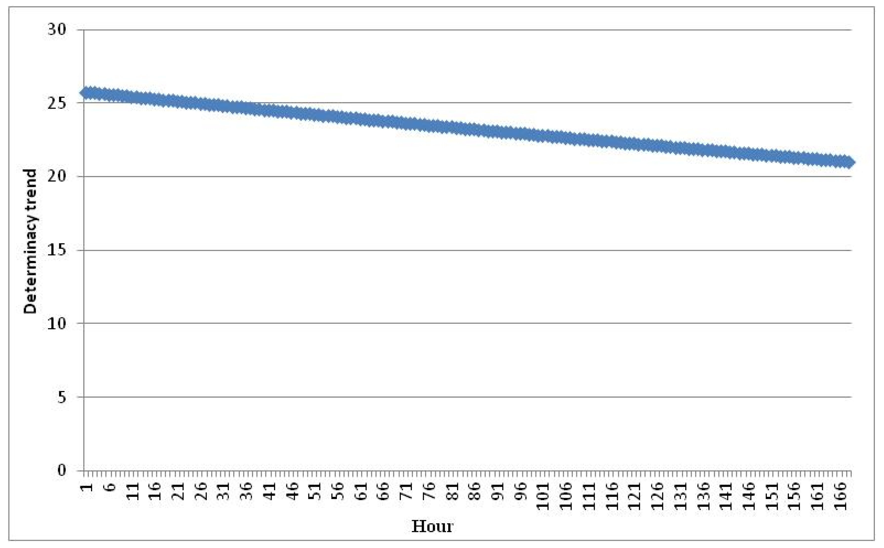
Figure 4.
Cyclic item and stochastic impact term in the natural form of the electricity price.

Figure 5.
The prediction results of different forecasting models and actual electricity price.

Table 1.
The first order stationary examination results for the logarithmic form of the original 168 h electricity price data.
Table 1.
The first order stationary examination results for the logarithmic form of the original 168 h electricity price data.
| Data Series | Examination For (C,T,K) | Augmented Dickey–Fuller (ADF) Test Result | p Value | Conclusion |
|---|---|---|---|---|
| (N,N,1) | −0.631624 | 0.1221 | Unstable | |
| (N,N,0) | −12.090678 | 0.0000 | stable |
Table 2.
The optimal values of ‘σ2‘ and ‘c’ in whale optimization algorithm-least square support vector machine (WOA-LSSVM) for deterministic trend forecasting, periodic item forecasting and stochastic term forecasting.
Table 2.
The optimal values of ‘σ2‘ and ‘c’ in whale optimization algorithm-least square support vector machine (WOA-LSSVM) for deterministic trend forecasting, periodic item forecasting and stochastic term forecasting.
| Parameters | LSSVM for Determinacy Trend | LSSVM for Cyclic Item | LSSVM for Random Term |
|---|---|---|---|
| σ2 | 3.9972 | 8.6573 | 6.8014 |
| c | 97.146 | 93.867 | 94.156 |
Table 3.
Root mean square error (RMSE) and mean absolute percentage error (MAPE) of WOA-LSSVM for each hour.
Table 3.
Root mean square error (RMSE) and mean absolute percentage error (MAPE) of WOA-LSSVM for each hour.
| Error Criteria | MAPE | RMSE | |
|---|---|---|---|
| Hours | |||
| 1 | 0.03% | 0.007 | |
| 2 | 0.26% | 0.055 | |
| 3 | 0.38% | 0.081 | |
| 4 | 0.43% | 0.091 | |
| 5 | 1.31% | 0.286 | |
| 6 | 0.23% | 0.052 | |
| 7 | 1.18% | 0.381 | |
| 8 | 0.37% | 0.128 | |
| 9 | 1.11% | 0.345 | |
| 10 | 0.74% | 0.228 | |
| 11 | 0.04% | 0.012 | |
| 12 | 0.12% | 0.034 | |
| 13 | 0.93% | 0.237 | |
| 14 | 0.09% | 0.023 | |
| 15 | 0.60% | 0.145 | |
| 16 | 0.73% | 0.177 | |
| 17 | 0.19% | 0.052 | |
| 18 | 0.86% | 0.274 | |
| 19 | 0.28% | 0.088 | |
| 20 | 0.29% | 0.084 | |
| 21 | 0.02% | 0.006 | |
| 22 | 0.81% | 0.201 | |
| 23 | 1.40% | 0.319 | |
| 24 | 0.50% | 0.102 | |
| Average values | 0.54% | 0.182 | |
Table 4.
Values of ‘σ2‘ and ‘c’ for comparison approaches.
| Parameters | B-N-D-LSSVM | B-N-D-FOA-LSSVM | B-N-D-PSO-LSSVM | WOA-LSSVM | ||||||
|---|---|---|---|---|---|---|---|---|---|---|
| Determinacy Trend | Cyclic Item | Random Term | Determinacy Trend | Cyclic Item | Random Term | Determinacy Trend | Cyclic Item | Random Term | ||
| σ2 | 4.0102 | 7.3657 | 8.0241 | 3.7067 | 9.0236 | 7.937 | 3.9889 | 8.2489 | 6.0124 | 5.0124 |
| c | 99.156 | 95.086 | 92.303 | 94.302 | 94.137 | 91.262 | 96.103 | 92.989 | 95.112 | 94.879 |
Table 5.
The results of MAPE and RMSE for all models testing on the hourly electricity price data on 18 December 2017.
Table 5.
The results of MAPE and RMSE for all models testing on the hourly electricity price data on 18 December 2017.
| Error Criteria | B-N-D-WOA- | B-N-D-PSO- | B-N-D-FOA- | B-N-D- | B-N-D- | WOA-LSSVM |
|---|---|---|---|---|---|---|
| LSSVM | LSSVM | LSSVM | LSSVM | ARIMA | ||
| MAPE | 0.54% | 1.44% | 2.76% | 3.07% | 5.58% | 5.77% |
| RMSE | 0.18 | 0.46 | 0.85 | 1.04 | 1.90 | 2.79 |
Table 6.
The results of MAPE and RMSE for all models testing the hourly electricity price data on 22 January 2018.
Table 6.
The results of MAPE and RMSE for all models testing the hourly electricity price data on 22 January 2018.
| Error Criteria | B-N-D-WOA- | B-N-D-PSO- | B-N-D-FOA- | B-N-D- | B-N-D- | WOA-LSSVM |
|---|---|---|---|---|---|---|
| LSSVM | LSSVM | LSSVM | LSSVM | ARIMA | ||
| MAPE | 0.80% | 1.76% | 2.52% | 3.88% | 6.03% | 6.72% |
| RMSE | 0.24 | 0.78 | 1.03 | 1.69 | 2.21 | 3.86 |
Table 7.
The results of MAPE and RMSE for all models examining the hourly electricity price data on 21 February 2018 to 25 February 2018.
Table 7.
The results of MAPE and RMSE for all models examining the hourly electricity price data on 21 February 2018 to 25 February 2018.
| Error Criteria | B-N-D-WOA- | B-N-D-PSO- | B-N-D-FOA- | B-N-D- | B-N-D- | WOA-LSSVM |
|---|---|---|---|---|---|---|
| LSSVM | LSSVM | LSSVM | LSSVM | ARIMA | ||
| MAPE | 0.71% | 1.65% | 2.61% | 3.55% | 5.87% | 6.41% |
| RMSE | 0.22 | 0.62 | 1.14 | 1.34 | 2.13 | 3.59 |
© 2018 by the authors. Licensee MDPI, Basel, Switzerland. This article is an open access article distributed under the terms and conditions of the Creative Commons Attribution (CC BY) license (http://creativecommons.org/licenses/by/4.0/).
Share and Cite
MDPI and ACS Style
Zhao, H.; Guo, S.; Zhao, H. A Multi-Stage Intelligent Model for Electricity Price Prediction Based on the Beveridge–Nelson Disintegration Approach. Sustainability 2018, 10, 1568. https://doi.org/10.3390/su10051568
AMA Style
Zhao H, Guo S, Zhao H. A Multi-Stage Intelligent Model for Electricity Price Prediction Based on the Beveridge–Nelson Disintegration Approach. Sustainability. 2018; 10(5):1568. https://doi.org/10.3390/su10051568
Chicago/Turabian StyleZhao, Haoran, Sen Guo, and Huiru Zhao. 2018. "A Multi-Stage Intelligent Model for Electricity Price Prediction Based on the Beveridge–Nelson Disintegration Approach" Sustainability 10, no. 5: 1568. https://doi.org/10.3390/su10051568
Note that from the first issue of 2016, this journal uses article numbers instead of page numbers. See further details here.