Modeling Global Trade in Phosphate Rock within a Partial Equilibrium Framework


Ecosystems Services and Management Program (ESM), International Institute for Applied Systems Analysis (IIASA), Schlossplatz 1, Laxenburg A-2361, Austria
*
Author to whom correspondence should be addressed.
Sustainability 2018, 10(5), 1550; https://doi.org/10.3390/su10051550
Submission received: 23 March 2018
/
Revised: 4 May 2018
/
Accepted: 8 May 2018
/
Published: 14 May 2018
(This article belongs to the Special Issue Phosphorus Circular Economy: Closing Loops through Sustainable Innovation)
Abstract
:Against the background of combined population and consumption growth, the global sustainable development agenda foresees limits to the expansion of agricultural land. The application of fertilizer is necessary to replenish soil nutrients and keep crop yields high. Phosphate rock (PR) is the main raw material for the production of commercial phosphorus fertilizers. The international PR market is highly concentrated in terms of reserves and supply: a few countries export the major share of all PR traded globally. As many countries are highly dependent on phosphorus import, the modeling of international PR trade and thus exploration of what-if scenarios is of great interest. For modeling purposes, we employ the partial equilibrium framework. The model is driven by a subset of the United Nations (UN) Comtrade database at a yearly time step spanning the period 1997–2016. The only inputs to the model are slope coefficients of demand–supply curves. The transportation costs are internalized by creating a costs ensemble on the basis of historical data. While reasonably sensitive to its inputs, the model fits very well to reported global annual traded quantities and prices and considerably improves per-trade-partner quantity estimates as compared to simple period-averaging approaches. This is the first application of a partial equilibrium approach to global PR market modeling, including validation.
1. Introduction
Within the agenda of sustainable development goals (SDGs) [1], the agricultural economic sector plays an important role, as it is strongly linked to over half of the SDGs, including SDG 2: Zero Hunger; SDG 3: Good Health and Well Being; SDG 8: Decent Work and Economic Growth; SDG 12: Responsible Consumption and Production; and SDG 15: Life on Land, to name a few. The SDG 12 is directly linked to the principles of circular economy and sets a high priority for the reduction of the ecological footprint in agricultural production [2]. In this context, keeping crop yields at high levels is necessary to satisfy the growing food demand of the earth’s population and to limit agricultural expansion into natural land [3]. Fertilizer application is indispensable for replenishing nutrients in the soil that would otherwise quickly become depleted [4]. Phosphate rock (PR) is the main raw material for the production of commercial phosphorus fertilizers—diammonium phosphate, triple superphosphate, monoammonium phosphate, and complex fertilizers including the mixes thereof. The global PR market is very much concentrated: according to the 2008 and 2015 U.S. Geological Survey reports, over 90% of the total production quantity is mined by a handful of countries [5,6]. The global reserves of scarce PR resources are also highly concentrated, with about 75% of the world’s reserves being located in Morocco and Western Sahara, followed by 5% in China and 3% in Algeria [6]. The biggest PR supplier in the world market according to the trade statistics for 2007–2016 is Morocco with an average value of 22 Mtons/year, followed by Jordan with 8.5 Mtons/year and Russia with 6.7 Mtons/year [7]. Here and throughout we abbreviate million tons with Mtons. The biggest PR consumer in the world market by far, according to the trade statistics for 2007–2016, is India with 11.6 Mtons/year, followed by the United States with 5 Mtons/year and Brazil and Poland with 3 Mtons/year each [7].
The majority of countries are net importers of phosphorous, while some completely depend on its import; for example, in India “indigenous rock phosphate supplies meet only 5–10% of the total requirement of P2O5” according to Indian authorities [8]. Modeling of the international PR trade is therefore of great interest, and primary questions regard price sensitivity of the global market to supply shocks (e.g., triggered by potential instability in phosphorus export), increased demand (e.g., due to policy changes such as export/import taxes or subsidies [9]), and effects induced by the transportation sector. In addition to these substantive topics, there are also technical questions that have to be addressed before carrying out any meaningful analysis: (1) to what degree modeling is possible under the constraints of the present data availability and data quality; (2) if and how such a model could be validated. The rest of the paper describes the data harmonization process adopted to prepare the inputs for the model and presents the mathematical formulation of the model, the validation results, and the discussion of the implications for the modeling purposes stated above.
2. Materials and Methods
2.1. Data Preparation
The data source feeding the model is the United Nations (UN) Comtrade database [7], which contains per-commodity information on annual trade flows reported by countries, including the type of the trade flow (export or import), the trade partner (country), the quantity, and the trade value in U.S. dollars. Countries are supposed to report free-on-board (FoB) prices when exporting and cost, insurance, and freight (CIF) prices when importing goods [10]. Unfortunately, the quality of the UN Comtrade data is known to be poor, so that CIF/FoB rates are of questionable quality and are not usable as such [11,12]. A vivid indication of the data quality issue is the fact that one study found that only 10% of the CIF/FoB ratios lay in the plausible range [11]. Unfortunately, as the exploration of the data contained within the UN Comtrade shows, the quality has not improved greatly since these analyses were published. The inconsistencies, which particularly regard PR, include (1) missing records (e.g., only one of the trade partners reports on a trade flow, but the other does not); (2) quantities reported as exported do not match imported quantities for a pair of reporting countries; and (3) CIF and FoB prices derived from reported values of goods are inconsistent, so that the CIF is less than the FoB price. The presence of these inconsistencies leads to the necessity of data harmonization before this data can be used for modeling.
Although there exists a UN Comtrade based product—the BACI World Trade Database [13]—that is available to subscribers, we independently carried out a similar data harmonization of the original UN Comtrade data. The reason for implementing the data harmonization procedure specifically for PR was to obtain a fine control at each of the data processing steps and to keep track of these modifications. The key data processing steps are described in detail below:
- Initial import of a raw dataset into a database.
- Simplification by filtering out very small trades.
- Harmonization of bilateral traded quantities.
- Subsetting data on the basis of major exporters and importers.
- Fitting a regression of transportation costs on distance.
- Corrections of CIF and FoB prices.
As an initial step, we imported the original comma-separated file provided by the UN Comtrade into a SQLite database [14]. The imposed data consistency constraints (non-empty fields) led to the successful import of 98.5% of the records (22,280 out of 22,619) for the full time period (1986–2016) available for PR. At the following step, we simplified the data by removing trade flows marked as re-export and -import (145 records, i.e., 0.65%), leaving 99.35% of records (22,135) untouched—or 99.94% when expressed in terms of weight. We further simplified the dataset by eliminating records with very small traded quantities—those below 1 Kton/year (here and further 1 Kton is 1000 ton), reducing the number of records down to 8542 (38.59%), yet maintaining 99.33% when expressed in terms of weight.
At the first stage of the data harmonization procedure, we added missing data: those records for which only the exporter or importer (but not both) had reported a trade were supplemented with reciprocal records carrying the same traded quantity. The records for which the imported quantity did not match the exported quantity were adjusted by taking the maximum of the two reported quantities, while the value of exported or imported goods was adjusted to represent the respective original FoB or CIF price. At this step, we added 3678 records (43.06%), or 31.11% in terms of weight. That quantity was added rather “virtually”—it was not missing from the database completely, but only in the report of one of the two trading partners.
For running the model, we used a subset of the so far harmonized database corresponding to the 20 year period spanning the years 1997–2016. The reason for selecting a narrower period was that it was relatively stable in terms of major PR exporters and at the same time was reasonably long for model validation purposes. In the preceding years, 1990–1997, the annual PR export from the United States dropped 10-fold from 5 to 0.5 Mtons/year, which effectively led to the United States losing the status of a major world PR exporter. In order to keep the size of the model reasonable, we reduced the number of trading partners and selected the 12 largest exporters (country ISO codes: MAR, JOR, RUS, SYR, CHN, EGY, ISR, TGO, DZA, PER, KAZ, and TUN) and 25 largest importers (country ISO codes: IND, USA, BRA, POL, BEL, ESP, IDN, NLD, MEX, KOR, LTU, NZL, TUR, JPN, NOR, AUS, FRA, LBN, UZB, MYS, BGR, PHL, UKR, CAN, and BLR), with an additional requirement for a trade flow to be greater than 10 Kton/year. This covered 34.99% of the trade flows (active exporter–importer tuples) over the modeling period 1997–2016, and 80.74% in terms of the total traded PR quantity over the period. The resulting dataset contained information on 12 major exporters and 25 major importers, with matching traded annual quantities that were greater than 10 Kton/year. The state of the data at this point is further referred to by the “point-zero” dataset.
An indicative estimate of the number of records and traded weight left in the point-zero dataset from the original dataset spanning the same time period 1997–2016 is as follows:
While the number of records dropped significantly, over 80% of the traded quantity was represented in the data. This estimate is given under the assumption that the simplification by removing the re-export and -import flows and small quantities affected the periods before and after 1997 in a comparable way. In this calculation, we were not taking into account “virtually” added missing data, only removed data. We also did not take into account the percentage of successfully imported records at the initial import step, as it was difficult to qualify records not reporting anything in terms of quantity and/or trade value.
At the second stage of the data harmonization procedure, we aimed to achieve consistent values of both CIF and FoB prices and transportation costs for any trade, where possible. In order to do so, we derived a plausibility criteria for the estimated transportation cost and then applied this criteria for correcting the point-zero dataset. First, we removed from the database records that were inconsistent, as these implied a FoB price greater than the CIF price. This removed about 19.08% of the records; that is, it left 80.92% of records, or 85.09% in terms of traded weight. A loose requirement for both CIF and FoB prices to be within the “reasonable” range of 15–1500 $US/ton and for the transportation cost not to exceed 200 $US/ton left 80.09% of the records, or 88.32% in terms of weight.
The justification for loosely setting the lower threshold to 15 $US/ton was that the global PR production cash cost (excluding financing costs), in 1983, was in the range of 16–55 $US/ton ex-mine and, in 2013, was in the range of 13–94 $US/ton [15]. The justification for loosely setting the upper threshold to 1500 $US/ton was that historical PR prices were below 500 $US/ton [16]. The justification for loosely setting the upper threshold for the transportation costs to 200 $US/ton was that the maximum international PR transport cost (Red Sea—Indonesia) reported in 2012 was below 30 $US/ton [17,18]. The 2018 quote for the PR transport cost was below 100 $US (Jordan–Indonesia) [19]. This quote is openly available and likely is an overestimation of the real cost, as it does not take into account possible long-term agreements and trust built between a transportation company and a PR producer.
On the basis of these records (also satisfying the FoB ≤ CIF price condition), we estimated a linear regression of transportation cost on distance between trading countries. The source of distance data is the GeoDist database [20]. The estimated linear regression provides information on the “average” transportation cost, and in order to use this information for harmonizing the database, we imposed a minimum threshold of 25% and maximum threshold of 500% of the average cost for a transportation cost to be deemed plausible.
As this regards the dataset used for deriving the transport cost regression, an indicative estimate of the number of records and traded weight left in them from the original dataset is as follows:
Here we estimated the numbers on the basis of those for the base point-zero dataset.
In the final stage of the harmonization procedure, we carried out corrections to the point-zero dataset by employing information on the transportation cost thresholds, as follows. If both CIF and FoB prices were within the “reasonable” range of 15–1500 $US/ton but the transportation cost was out of bounds, that is, lower than 25% or higher than 500% of average, then the corrected prices were calculated using the following formulas:
where is the average transportation cost corresponding to the distance. If only one price, for example, FoB, was “reasonable” while the other (CIF) was not, the applied correction was
If, on the contrary, the CIF price was “reasonable” while the FoB price was not, the applied correction was analogous:
If neither the CIF nor FoB price was “reasonable”, then the record was discarded from the resulting database. The statistics for the final-stage corrections relative to the point-zero dataset were as follows: 40.2% of records were corrected (including removals), and in this course, 30.2% of the volume was affected (including removals). The detailed correction statistics by the type of correction are presented in Table 1. The harmonized dataset for the 12 exporters and 25 importers obtained at this final stage of the harmonization procedure is further referred to as the “fully harmonized” dataset.
A comparison of global weighted CIF and FoB prices calculated from the fully harmonized dataset against those derived from the original UN Comtrade data and historical World Bank PR prices [21] is presented in Figure 1. It shows that in spite of the modifications carried out, the original global weighted CIF and FoB prices were negligibly affected, particularly when compared to an alternative price estimate provided by the World Bank.
2.2. Model Description
To model international PR trade, we employed a partial equilibrium framework that is widely used in economic modeling [22,23,24]. In our problem setting, changes in traded quantities and prices were induced by changes in the demand–supply of trading partners and changes in transportation costs. However, the only inputs to the model were annual slope coefficients of demand–supply. The need for estimating annual transportation costs was eliminated by employing a representative set of historical data. An ensemble of optimization models for which each employed one of the possible annual transportation cost estimates comprised the entire model. A single optimization problem was formulated as follows:
where letters “c” and “s” mark consumers ( countries) and suppliers ( countries), respectively; and are countries’ demand and supply functions, respectively; are bilateral traded quantities; are transportation costs; and and are historical maxima of traded quantities. In order to obtain an estimated value (price or quantity), the respective models’ outputs were averaged over the individual members of the ensemble (Equation (1)).
To approximate the annual demand and supply, linear functions were employed:
where parameters , , , and depend on the year and were determined by the following equations:
where (or ) is the imported (or exported) quantity and (or ) is the import (or export) price of an importer (or exporter) in a particular year. We set the value of to the maximum historically observed import price of the respective importer +10%. We assumed that for the purposes of demand curve approximation, this represented the virtual (maximum) price an importer would pay for a “very small” quantity. For the purposes of supply curve approximation, we set to zero the virtual price for which exporters would sell a “very small” amount of PR. From a technical perspective, the simplifying assumption helped to prevent degradation of the problem (Equation (1)) by making sure that all supply functions (price depending on quantity) were strictly increasing while annual demand functions by their construction were strictly decreasing.
3. Results
A linearization of the problem (Equation (1)) could be carried out by approximating countries’ demand and supply functions and with piecewise constant functions. This technical modification allowed for a straightforward numerical solution of the respective linear programming (LP) problem, for example, by using the GLPK software [25]. The problem (Equation (1)) has an implicit time dimension—the year for which the equations are valid. In order to reduce the number of model input parameters, which was useful for the construction of compact exploratory scenarios, we substituted true transportation costs in a particular year with a set of transportation costs from other years, employing these as proxies for the true transportation costs that were not included in an exploratory scenario. By carrying out the transport costs’ substitution for a particular year, we created an ensemble of models (Equation (1)) that differed from each other only in transportation costs; their demand–supply curves were the same and corresponded to their linear approximation (Equation (2)) for that same year. The model by construction delivered exact exported and imported quantities by each exporter and importer for any year if true transportation costs for that year were used to run the model.
Our aim was to model exported and imported quantities and PR price only on the basis of demand–supply curves’ estimation for exporters and importers without having to deal with the transportation cost. By introducing the simple linear approximation of demand–supply curves (Equations (2) and (3)), we effectively reduced this parametrization to just a single parameter per country—the line slope.
In order to benchmark the resulting model, we employed two alternative approaches: (1) using just an average of the exported/imported quantities per country calculated over 1997–2016, further referred to as “Avg97-16”; and (2) using one of the years 1997–2016 for estimating exported/imported quantities by country in all other years and averaging this “naive” ensemble, further referred to as “AvgEns Naive”. As opposed to these simple approaches, the optimization–based averaged model ensemble was comprised of linearized problems (Equation (1)), for which true transportation costs for a particular year were excluded from the set of “plausible” transportation costs; this is further referred to as “AvgEns LP”. This exclusion represents a “leave-one-out cross-validation” approach, which in our particular case reflects an assessment scenario of an expert-based year-specific projection of future demand–supply without a respective projection of transportation costs. The leave-one-out cross-validation approach is commonly used if a dataset available for model validation is small [26]; this was exactly our case, as the dataset was limited to the time period 1997–2016, giving only 20 data points (years).
The modeling results are illustrated in Figure 2, and the respective summary statistics are presented in Table 2. The mean absolute errors (MAEs) of individual models in estimated exported quantity by country relative to total exported quantity for a given year are depicted by circles and crosses for the AvgEns Naive and AvgEns LP ensembles, respectively. The lines represent MAEs of Avg97-16 and ensemble averages (AvgEns Naive and AvgEns LP). Table 2 proves the value delivered by the suggested optimization-based modeling approach: while the minimum, average, and maximum MAEs of both Avg97-16 and AvgEns Naive are close to each other, AvgEns LP reduced all of these MAEs by over 50%.
The modeling results for PR importers are illustrated in Figure 3, and the respective summary statistics are presented in Table 3. The MAEs of individual models in estimated imported quantity by country relative to total exported quantity for a given year are depicted by circles and crosses for the AvgEns Naive and AvgEns LP ensembles respectively. The lines represent the MAEs of Avg97-16 and the ensemble averages (AvgEns Naive and AvgEns LP). Table 3 gives the value delivered by the suggested optimization-based approach also for modeling importers: while the minimum, average, and maximum MAEs for both Avg97-16 and AvgEns Naive are close to each other, AvgEns LP reduced the minimum and average MAEs by about 50% and the maximum MAE by about 30%.
Figure 3 illustrates two interesting anomalies: (1) the model under-performed in terms of per-country quantities as compared to both benchmarks in the price peak year 2008, and (2) the model performance suffered in the following year (2009) while still being better than the benchmarks (see also Figure 2). The analysis of indicators depicted in Figure 4 helps to shed some light on possible causes of these anomalies.
Both the global transportation cost and the number of trade flows (exporter–importer pairs) reached historical (1997–2016) maximums in 2008, while in the following year, the number of trade flows dropped to a historical minimum, and at the same time, the by-country sum of changes in exported quantities to the previous year increased to a historical maximum. The model was challenged when reproducing by-country quantities for 2008 and 2009, as these years were quite specific in terms of their trade flow network configuration, and 2008 in addition was also specific in terms of transportation cost; thus the set of transportation costs (that did not include “true” transportation costs for a particular year, only “plausible” costs) was less representative for these years.
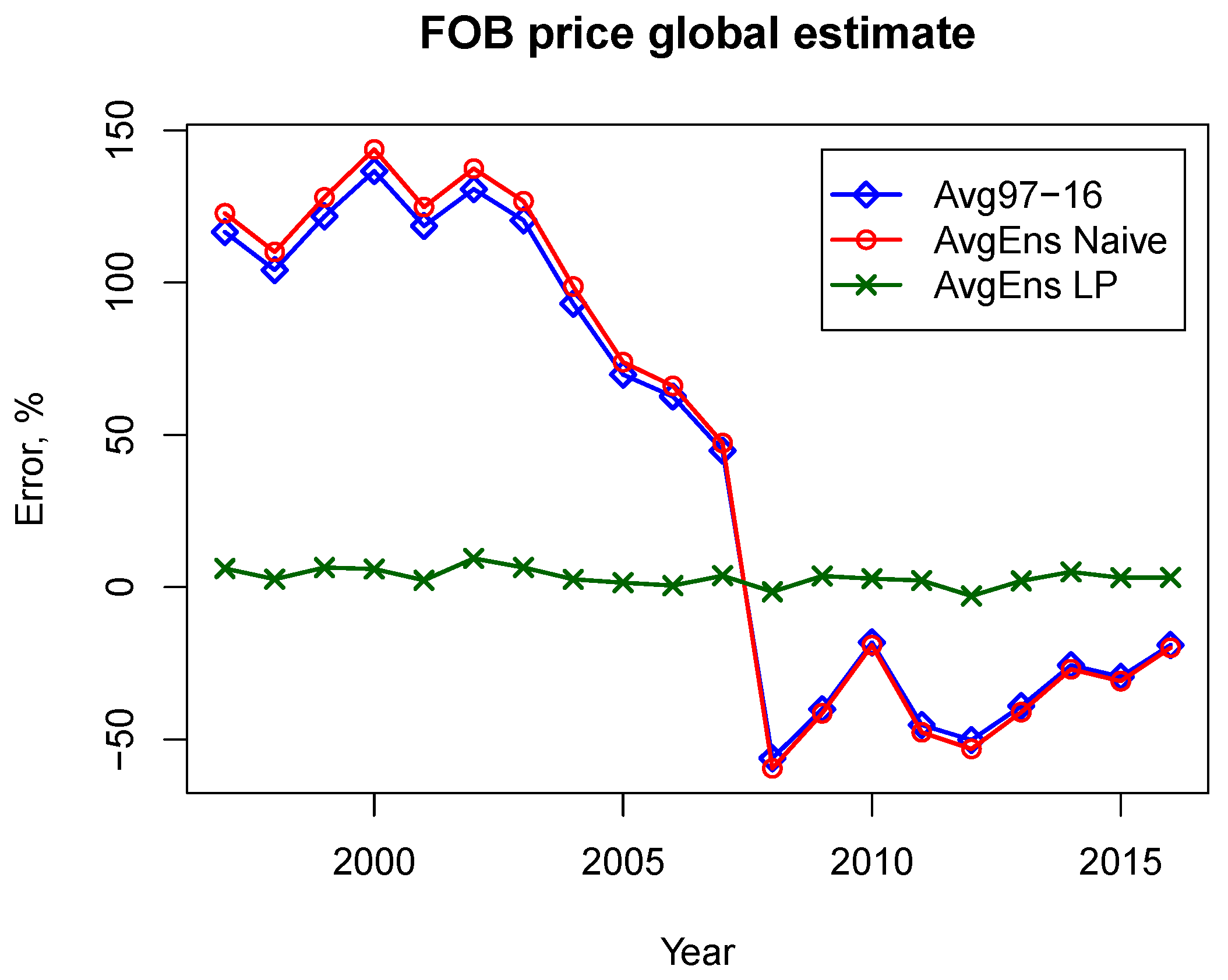
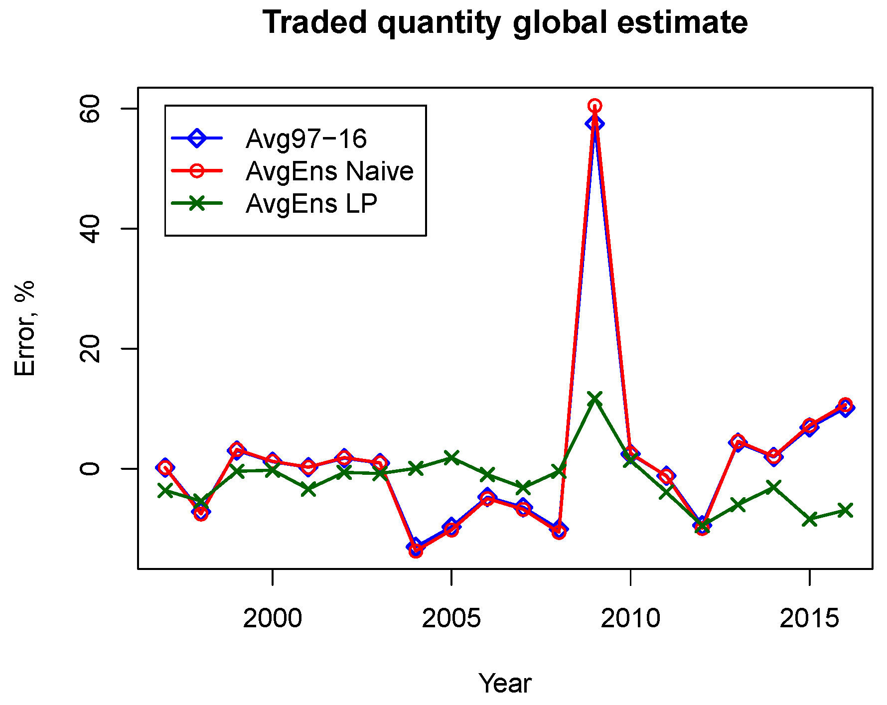
While errors in the model output at a country-level increased in turbulent years, the accuracy of the model’s global estimates remained stable over the entire period and by far exceeded that of both benchmarks Avg97-16 and AvgEns Naive, including for the price peak year 2008. Thus, over the entire modeling period 1997–2016, the maximum absolute value of the error in the global FoB price estimate was 9.42% (Figure 5), the maximum absolute value of the error in the global CIF price estimate was 11.95% (Figure 6), and the maximum absolute value of the error in the global traded quantity estimate was 11.69% (Figure 7).
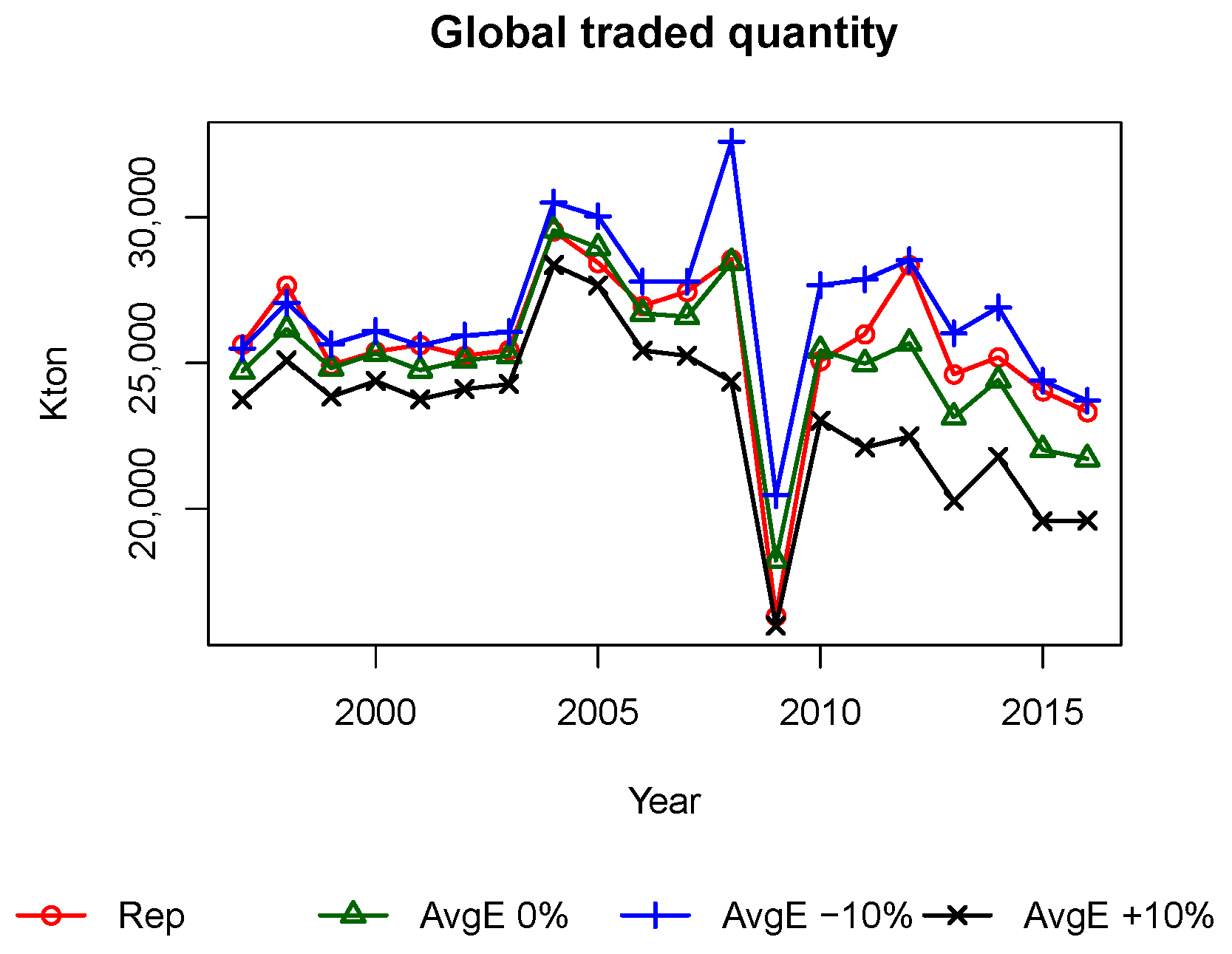
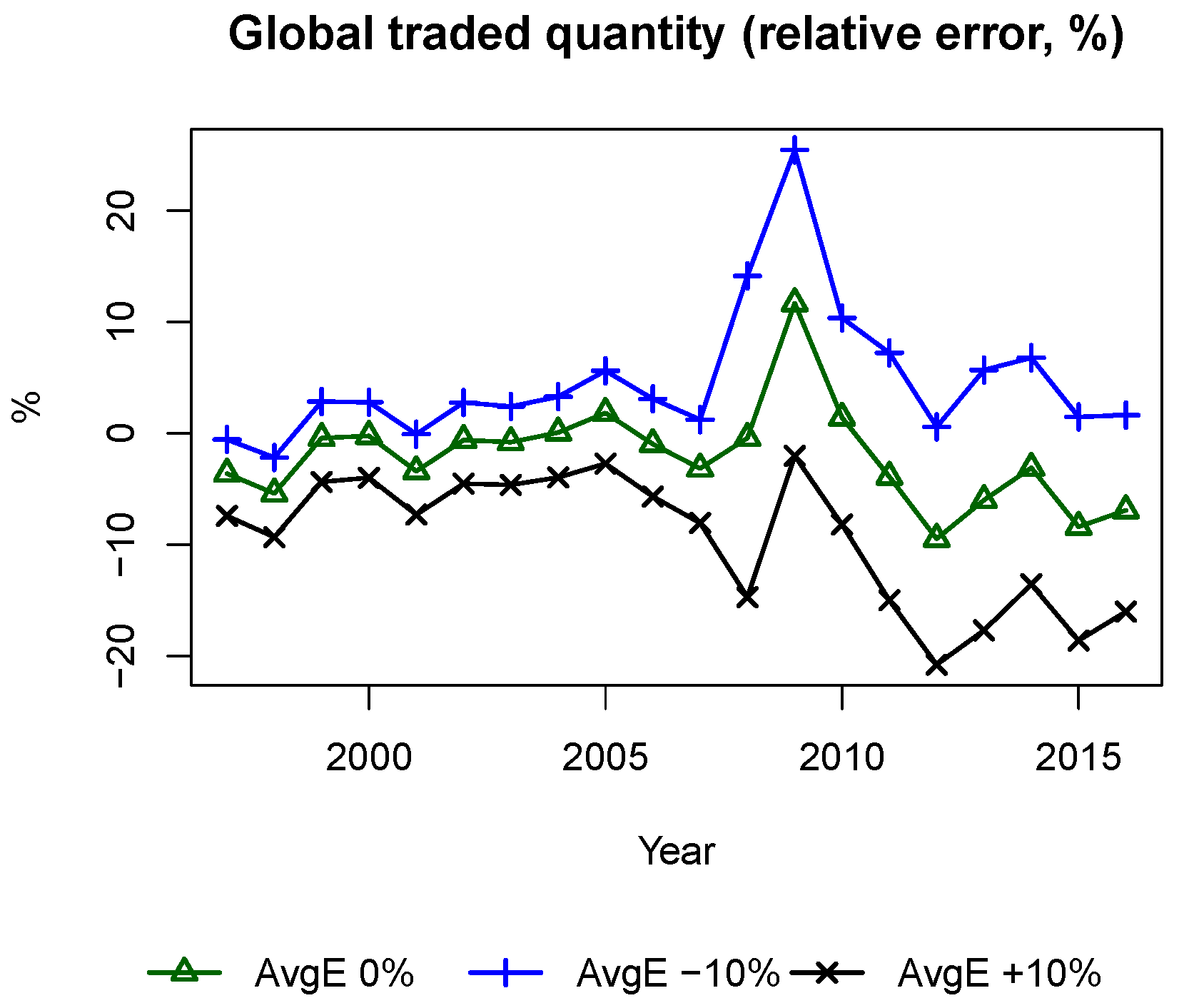
The model demonstrated reasonable sensitivity to errors in input data, that is, slope estimates of the demand–supply curves. For a sensitivity test, we constructed two extreme perturbations of demand–supply: (1) all supply curves were lowered by 10%, and demand curves were lifted by 10% (further referred to as “AvgE-10%”); and (2) all supply curves were lifted by 10%, and demand curves were lowered by 10% (further referred to as “AvgE+10%”). The respective errors in the global CIF and FoB price estimates over the entire modeling period 1997–2016 did not exceed 16% in absolute value, as depicted in Figure 8 and Figure 9. The value of the error in the global traded quantity remained within the approximate range from % to %, as illustrated in Figure 10 and Figure 11.
4. Discussion
The 20 year period 1997–2016 used for the model runs can be potentially extended. The fact that this period is relatively stable in terms of a set of major PR exporters and that the United States effectively dropped out from this set just before 1997 allowed for a clear separation between exporters and importers, as these sets of countries do not overlap. Theoretically, this constraint can be relaxed by expanding the modeling to selected domestic markets for estimation of a country’s preferences on exporting PR over importing it. However, the modeling of a domestic market in this context seems to be a major challenge and would imply a substantial complication of the model.
The modeling of the global PR market is relevant for addressing food security in the context of phosphorus, as high prices may limit access of certain importers to this non-renewable resource (and consequently P-fertilizer), potentially limiting their crop yields. The suggested model allows for the analysis of potential supply and demand shock scenarios in terms of their impact on prices and traded volumes. However, a per-scenario justification of the location and scale of plausible demand/supply shocks would require analysis of the aspects beyond the scope of the manuscript (e.g., national policies [9]) and therefore is left for future research.
The poor quality of trade data led to the necessity of intensive data pre-processing before that data could be used to feed the model. The initial stage of data harmonization was based on straightforward consistency rules and was not tailored in any way to the follow-up modeling exercise. The extensive modification of the original dataset transformed it into a consistent state. However, as consistency does not necessarily imply correctness, the modeling results and further interpretations have to be treated with caution. We applied several thresholds in the process of data harmonization and also when selecting a subset of trading partners. There may be potential to improve the model by adjusting the thresholds suggested as a reasonable first approximation.
In the first stage of the data harmonization procedure, when adding missing data to records for which only an exporter or importer (but not both) reported a trade, and also when taking the maximum of the records for which the imported quantity did not match the exported quantity (preserving the FoB or CIF price), we assumed there was no over-reporting in terms of quantity. If this were the case, however, more fine-tuned corrections would have been needed, requiring the utilization of additional data sources. As these were not available to us, we kept the aforementioned assumption.
We derived plausibility criteria for the estimated transportation cost from a relatively narrow dataset of filtered “reliable” records and then applied this criteria for correcting a relatively wide, less-filtered zero-point dataset. The idea behind this approach was to keep as much “reasonable” information from the original dataset as possible; that is, if just one of the prices (CIF or FoB) was plausible, the trade flow could be reasonably reconstructed.
The simplifying assumption in Equation (3) already briefly discussed above could be potentially modified so that the zero value is replaced by a lower PR mining cost, for example, 13 $US/ton, as reported for 2013 (or 16 $US/ton for 1983) [15]. However, from a theoretical perspective, this estimate is valid for a “substantially” greater than zero quantity. Another obstacle in employing this value is that this estimate is incompatible with the UN Comtrade data: in the period 1997–2003 (the years of relatively low PR prices), there were multiple trades reported at FoB prices equal or less than 13 $US/ton, totaling to 5.26% of the total reported exported volume over that time period. The data harmonization approach we carried out increased this value to 5.60%, hinting that these records were likely correct according to implemented filtering rules.
The assumption that transportation costs estimated for a particular year (within the modeling time period 1997–2016) were plausible also for any other year (i.e., for respective estimated demand–supply) was a simplification that allowed a stochastic interpretation of the model and exploitation of the model ensemble induced by a set of plausible transportation costs. As defined by the model structure, the modeling-error difference between the modeled values and those “correct” from the harmonized (and to a large degree, synthetic) dataset was due to this simplified assumption.
Although the model is able to reproduce exact exported (and imported) quantities by each exporter (and importer) for any year, provided that this year’s transportation costs are used to run the model, it cannot replicate quantities of bilateral trade. Bilateral trade data were not used for the model’s calibration; only the total annual traded quantity and price were part of the problem formulation (Equation (1)) in the demand–supply curves’ approximation (Equations (2) and (3)). As is stated for models of similar structure—partial equilibrium models—even if applied to a different economic sector of agriculture, difficulties in capturing changes at regional levels and regional results are much less satisfactory than the global results [22]. To a certain degree (depending on acceptable estimation error level), this applies to the results of our modeling (see Figure 2 and Figure 3). While sensitivity testing is common practice in presenting modeling results, a model validation is less common. That is particularly true for partial equilibrium and linear optimization models that “frequently receive only superficial validation” [24] or separate validation of single equations, not checking the model as a whole [23]. At the same time, the importance of validation increases as the models are applied for policy analyses [22]. In this context, the results presented in this paper stand out and validate the model as a whole.
5. Conclusions
This paper presents the results of modeling international PR trade within a partial equilibrium framework. Data harmonization and model validation received great attention. Throughout the data preparation procedure, we tracked the number of affected records in the database and respective physical volume. These data modifications at a record level did not affect the original global price.
The model formulated within a partial equilibrium framework allows for an efficient numerical solution through approximation by a LP problem. In the suggested modeling approach, the need for annual transportation cost estimation is eliminated by employing a model ensemble. The approximation of demand–supply curves is reduced to just a single slope parameter.
These simplifications greatly decrease the complexity of model parametrization. A scenario that can be assessed by the model consists of a set of demand–supply slope coefficients reflecting in a condensed way mining costs, policies, and expected profit levels of major exporters and importers. An alternative approach with a full linear approximation of demand–supply (slope and intercept) would need the number of parameters to be doubled. A full transportation cost estimation would need an estimation of many additional parameters (number of exporters multiplied by the number of importers), which greatly increases the complexity of an explorative scenario by adding challenges connected with transportation cost modeling.
The accuracy of modeled global estimates (price and quantity) was stable over the entire modeling period of 1997–2016 (including the turbulent years 2008 and 2009) and was by far superior to simple benchmarking approaches. This feature of the model together with its reasonable sensitivity to estimated demand–supply slope coefficients looks promising for the evaluation of rather extreme scenarios of PR market development. Such scenarios may represent economic, geopolitical, or policy-related shocks to demand–supply, including those triggered by technological innovations aimed at a transition towards circular economy. The construction of these scenarios and the analysis of their implications seems to be a promising direction for future research.
Author Contributions
M.O. provided the concept of the work. N.K. worked on data acquisition and mathematical modeling and drafted the manuscript. Both M.O. and N.K. carried out the analysis and interpretation of data and revised the manuscript.
Funding
This research was funded by the European Research Council Synergy Grant number 610028 Imbalance-P: Effects of phosphorus limitations on Life, Earth system and Society (Seventh Framework Programme of the European Union).
Acknowledgments
The authors acknowledge their colleagues Petr Havlik, Hugo Valin, Juraj Balkovic, and Ian McCallum from IIASA, Austria; Elena Moltchanova from the University of Canterbury, New Zealand; and Bernhard Geissler, Gerald Steiner, and Roland Scholz from Danube University Krems, Austria for useful discussions and help. The authors are thankful to four anonymous reviewers for their helpful feedback.
Conflicts of Interest
The authors declare no conflict of interest.
Abbreviations
The following abbreviations are used in this manuscript:
| CIF | Cost, insurance, and freight |
| ESM | Ecosystems Services and Management Program of IIASA |
| FoB | Free on board |
| IIASA | International Institute for Applied Systems Analysis |
| Kton | thousand ton |
| LP | Linear programming |
| PR | Phosphate rock |
| UN | United Nations |
References
- United Nations Development Programme. Sustainable Development Goals. 2016. Available online: http://www.undp.org/content/undp/en/home/sustainable-development-goals.html (accessed on 4 May 2018).
- United Nations Development Programme. Goal 12: Responsible Consumption and Production. 2016. Available online: http://www.undp.org/content/undp/en/home/sustainable-development-goals/goal-12-responsible-consumption-and-production.html (accessed on 4 May 2018).
- Foley, J.A.; DeFries, R.; Asner, G.P.; Barford, C.; Bonan, G.; Carpenter, S.R.; Chapin, F.S.; Coe, M.T.; Daily, G.C.; Gibbs, H.K.; et al. Global Consequences of Land Use. Science 2005, 309, 570–574. [Google Scholar] [CrossRef] [PubMed]
- Mueller, N.D.; Gerber, J.S.; Johnston, M.; Ray, D.K.; Ramankutty, N.; Foley, J.A. Closing yield gaps through nutrient and water management. Nature 2012, 490, 254–257. [Google Scholar] [CrossRef] [PubMed]
- The United States Geological Survey (USGS). Mineral Commodity Summaries; USGS: Reston, VA, USA, 2008.
- The United States Geological Survey (USGS). Mineral Commodity Summaries; USGS: Reston, VA, USA, 2015.
- UN Comtrade. International Trade Statistics Database. 2018. Available online: https://comtrade.un.org (accessed on 24 January 2018).
- Department of Fertilizers. Annual Report 2008–2009. 2009. Available online: http://fert.nic.in/sites/default/files/Annual-Report-2008-2009-english.pdf (accessed on 14 February 2018).
- Khabarov, N.; Obersteiner, M. Global Phosphorus Fertilizer Market and National Policies: A Case Study Revisiting the 2008 Price Peak. Front. Nutr. 2017, 4, 22. [Google Scholar] [CrossRef] [PubMed]
- International Chamber of Commerce. Incoterms 1953, International Rules for the Interpretation of Trade Terms. 1953. Available online: https://www.uncitral.org/pdf/english/texts_endorsed/INCOTERMS1953_e.pdf (accessed on 14 February 2018).
- Gaulier, G.; Mirza, D.; Turban, S.; Zignago, S. International Transportation Costs Around the World: A New CIF/FoB Rates Dataset. 2008. Available online: http://www.cepii.fr/baci_data/freight_rates/freight_rates_doc.pdf (accessed on 14 February 2018).
- Hummels, D.; Lugovskyy, V. Are Matched Partner Trade Statistics a Usable Measure of Transportation Costs? Rev. Int. Econ. 2006, 14, 69–86. [Google Scholar] [CrossRef]
- CEPII. BACI World Trade Database at A High Level of Product Disaggregation. 2018. Available online: http://www.cepii.fr/CEPII/en/bdd_modele/presentation.asp?id=1 (accessed on 15 February 2018).
- SQLite Developers. SQLite—A Self-Contained, High-Reliability, Embedded, Full-Featured, Public-Domain, SQL Database Engine. 2018. Available online: https://sqlite.org (accessed on 15 February 2018).
- Mew, M. Phosphate rock costs, prices and resources interaction. Sci. Total Environ. 2016, 542, 1008–1012. [Google Scholar] [CrossRef] [PubMed]
- IndexMundi. Rock Phosphate Monthly Price—US Dollars per Metric Ton. 2018. Available online: https://www.indexmundi.com/commodities/?commodity=rock-phosphate&months=360 (accessed on 21 February 2018).
- Bourne, I. (Ed.) Argus Fertilizer Freight: Weekly International Market Prices and Commentary. 2012. Issue 12-20. Available online: http://www.argusmedia.com/~/media/files/pdfs/fertilizers/argus-fertilizer-freight.pdf/?la=en (accessed on 25 January 2018).
- Bourne, I. (Ed.) Argus Fertilizer Freight: Weekly International Market Prices and Commentary. 2012. Issue 12-25. Available online: http://www.argusmedia.com/fertilizer/~/media/files/pdfs/samples/argus-fertilizer-freight.ashx (accessed on 25 January 2018).
- World Freight Rates. Freight Calculator: Rate Estimates for Port-to-Port Ocean Shipments. 2018. Available online: http://worldfreightrates.com/en/freight (accessed on 25 January 2018).
- Mayer, T.; Zignago, S. Notes on CEPII’s Distances Measures: The GeoDist Database. 2011. Available online: http://www.cepii.fr/CEPII/en/bdd_modele/presentation.asp?id=6 (accessed on 22 January 2018).[Green Version]
- Bank, T.W. DataBank Commodity Prices—History and Projections—Phosphate Rock, Nominal, $/mt. 2018. Available online: http://databank.worldbank.org/data/reports.aspx?source=3692&series=FPHOSROCK# (accessed on 22 February 2018).
- Baldos, U.L.C.; Hertel, T.W. Looking back to move forward on model validation: Insights from a global model of agricultural land use. Environ. Res. Lett. 2013, 8, 034024. [Google Scholar] [CrossRef]
- Mapila, M.A.; Kirsten, J.F.; Meyer, F.; Kankwamba, H. A Partial Equilibrium Model of the Malawi Maize Commodity Market; International Food Policy Research Institute (IFPRI): Washington, DC, USA, 2013; Volume 1254. [Google Scholar]
- McCarl, B.A.; Apland, J. Validation of linear programming models. South. J. Agric. Econ. 1986, 18, 155–164. [Google Scholar] [CrossRef]
- Makhorin, A. GNU Linear Programming Kit–Reference Manual for GLPK Version 4.64. 2017. Available online: https://www.gnu.org/software/glpk/ (accessed on 6 January 2018).
- Hastie, T.; Tibshirani, R.; Friedman, J. The Elements of Statistical Learning: Data Mining, Inference, and Prediction, 2nd ed.; Series in Statistics; Springer: Berlin, Germany, 2017. [Google Scholar]
Figure 1.
Global quantity-weighted CIF and FoB prices of phosphate rock (PR) calculated from the harmonized data (respectively denoted as “Hcif” and “Hfob”) and those derived from the original United Nations (UN) Comtrade dataset (respectively denoted as “Ocif” and “Ofob”) and historical World Bank PR prices (denoted as “WB”).
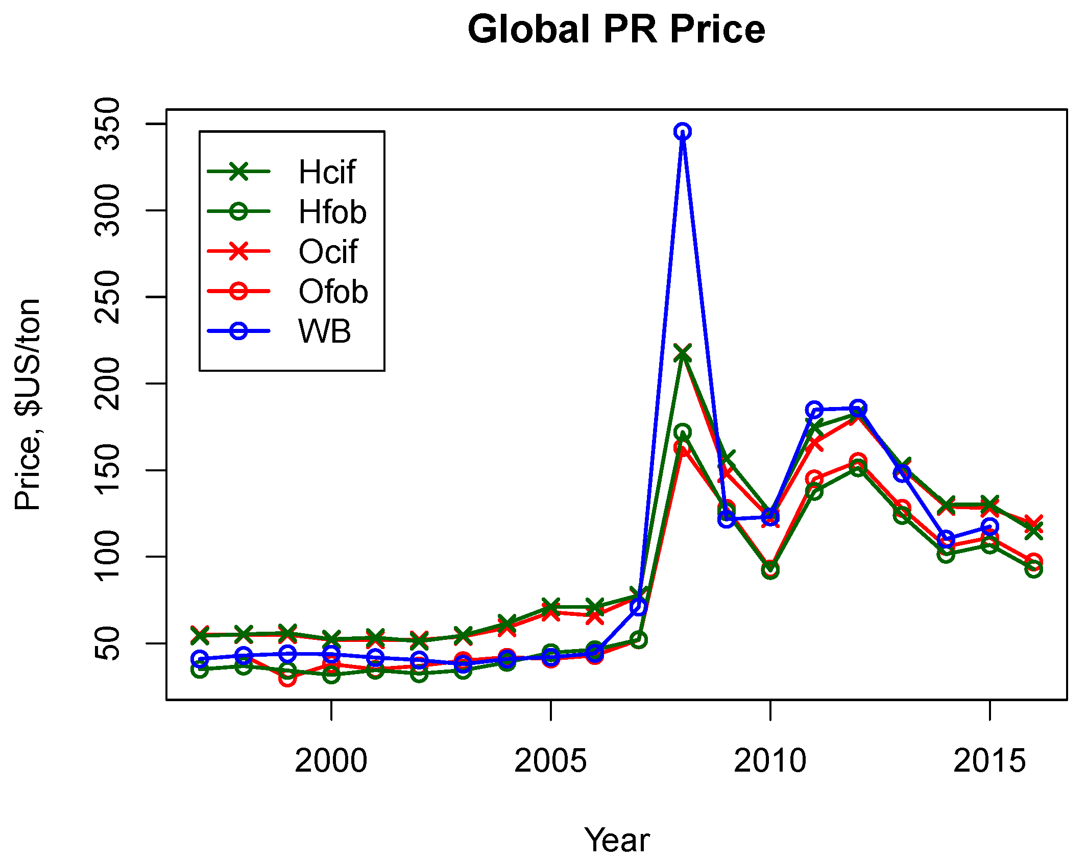
Figure 2.
Lines represent mean absolute errors (MAEs) of simple average over the period (“Avg97-16”) and naive and optimization-based ensemble averages (“AvgEns Naive” and “AvgEns LP”, respectively). The MAEs of individual models in estimated exported quantity by country relative to total exported quantity for a given year are depicted by circles and crosses for AvgEns Naive and AvgEns LP ensembles, respectively.
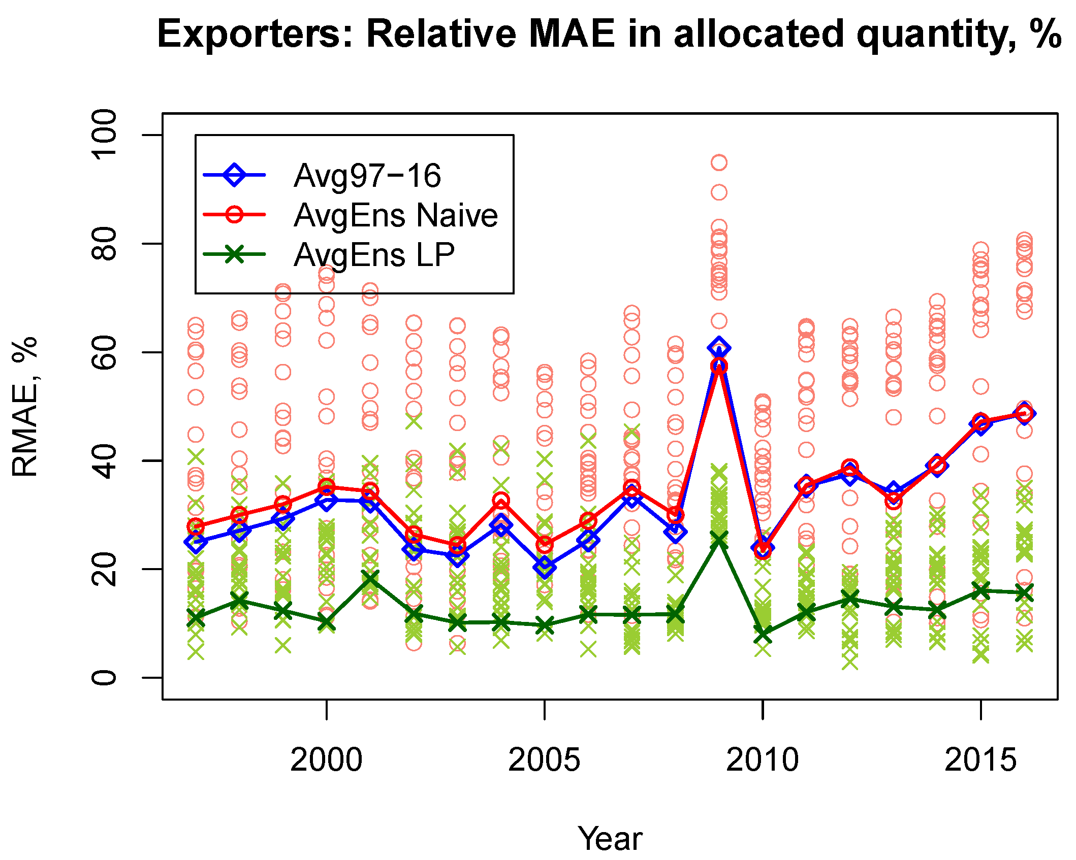
Figure 3.
Lines represent mean absolute errors (MAEs) of simple average over the period (“Avg97-16”) and naive and optimization-based ensemble averages (“AvgEns Naive” and “AvgEns LP”, respectively). The MAEs of individual models in estimated imported quantity by country relative to total imported quantity for a given year are depicted by circles and crosses for AvgEns Naive and AvgEns LP ensembles, respectively.
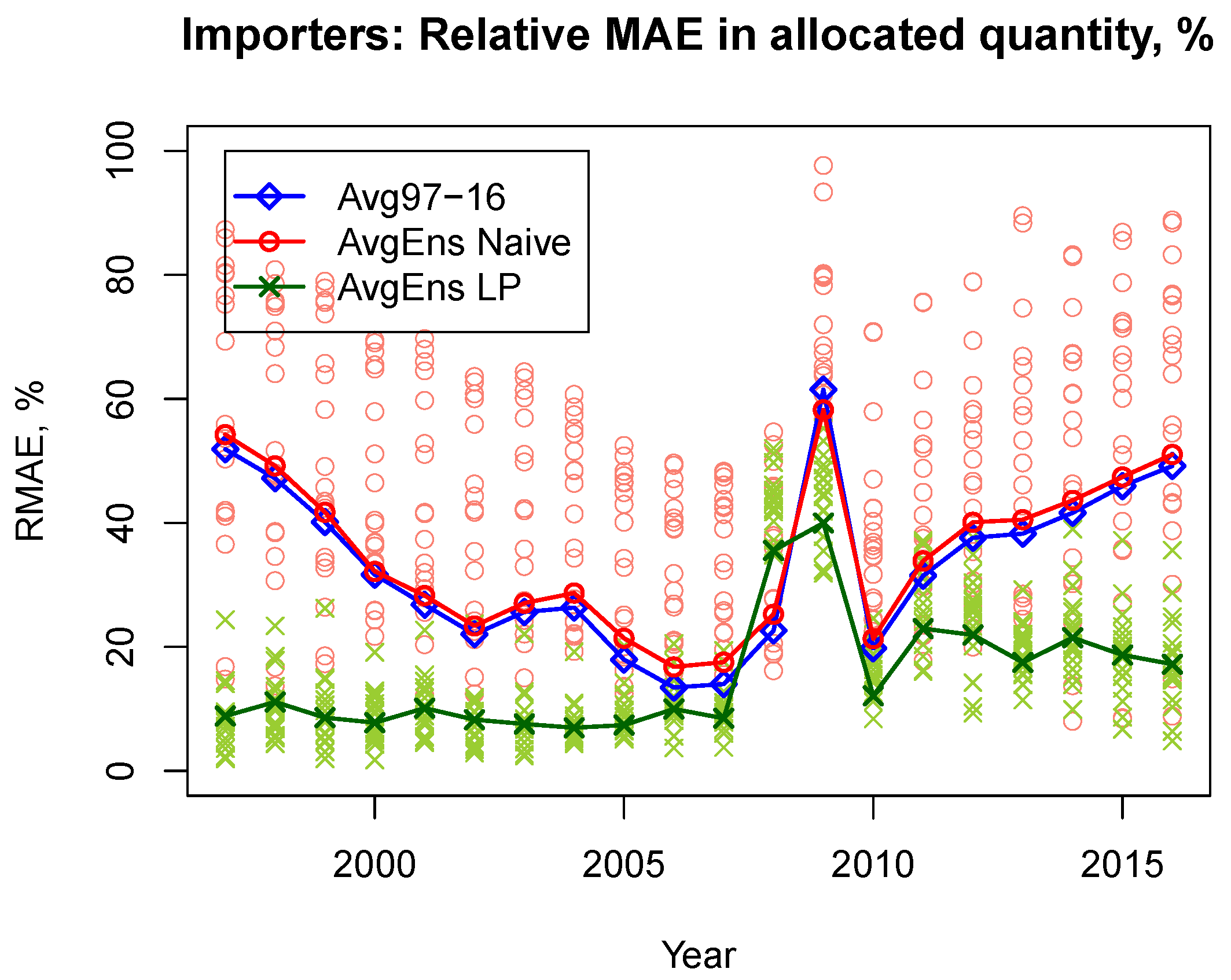
Figure 4.
Absolute deviation (%) from period average of global transportation cost (Tran.cost), the number of trade flows (Num.tr.fl.), and the by-country sum of changes in exported quantities to the previous year (Delta Qty).
Figure 4.
Absolute deviation (%) from period average of global transportation cost (Tran.cost), the number of trade flows (Num.tr.fl.), and the by-country sum of changes in exported quantities to the previous year (Delta Qty).

Figure 5.
Error in global phosphate rock (PR) free-on-board (FoB) price estimate by using a simple average over the period (“Avg97-16”), naive (“AvgEns Naive”), and optimization-based (“AvgEns LP”) ensemble averages.
Figure 5.
Error in global phosphate rock (PR) free-on-board (FoB) price estimate by using a simple average over the period (“Avg97-16”), naive (“AvgEns Naive”), and optimization-based (“AvgEns LP”) ensemble averages.

Figure 6.
Error in global phosphate rock (PR) cost, insurance, and freight (CIF) price estimate by using a simple average over the period (“Avg97-16”), naive (“AvgEns Naive”), and optimization-based (“AvgEns LP”) ensemble averages.
Figure 6.
Error in global phosphate rock (PR) cost, insurance, and freight (CIF) price estimate by using a simple average over the period (“Avg97-16”), naive (“AvgEns Naive”), and optimization-based (“AvgEns LP”) ensemble averages.
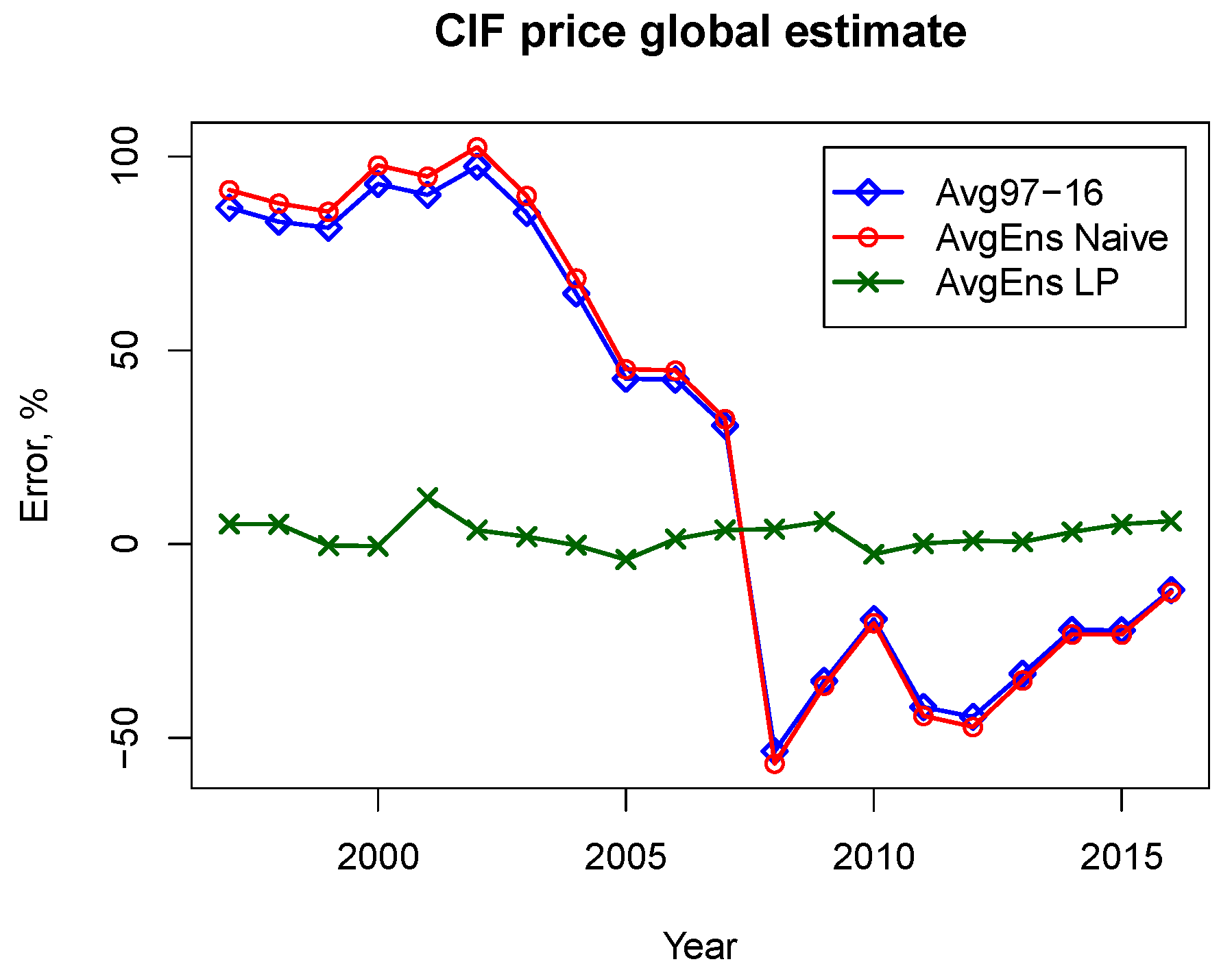
Figure 7.
Error in global phosphate rock (PR) traded quantity estimate by using a simple average over the period (“Avg97-16”), naive (“AvgEns Naive”), and optimization-based (“AvgEns LP”) ensemble averages.
Figure 7.
Error in global phosphate rock (PR) traded quantity estimate by using a simple average over the period (“Avg97-16”), naive (“AvgEns Naive”), and optimization-based (“AvgEns LP”) ensemble averages.

Figure 8.
Relative error in estimating global cost, insurance, and freight (CIF) price by unperturbed model ensemble “AvgE 0%”; an ensemble with supply curves shifted by −10% (demand curves lifted by 10%), “AvgE-10%”; and an ensemble with supply curves shifted by +10% (demand curves lowered by 10%), “AvgE+10%”.
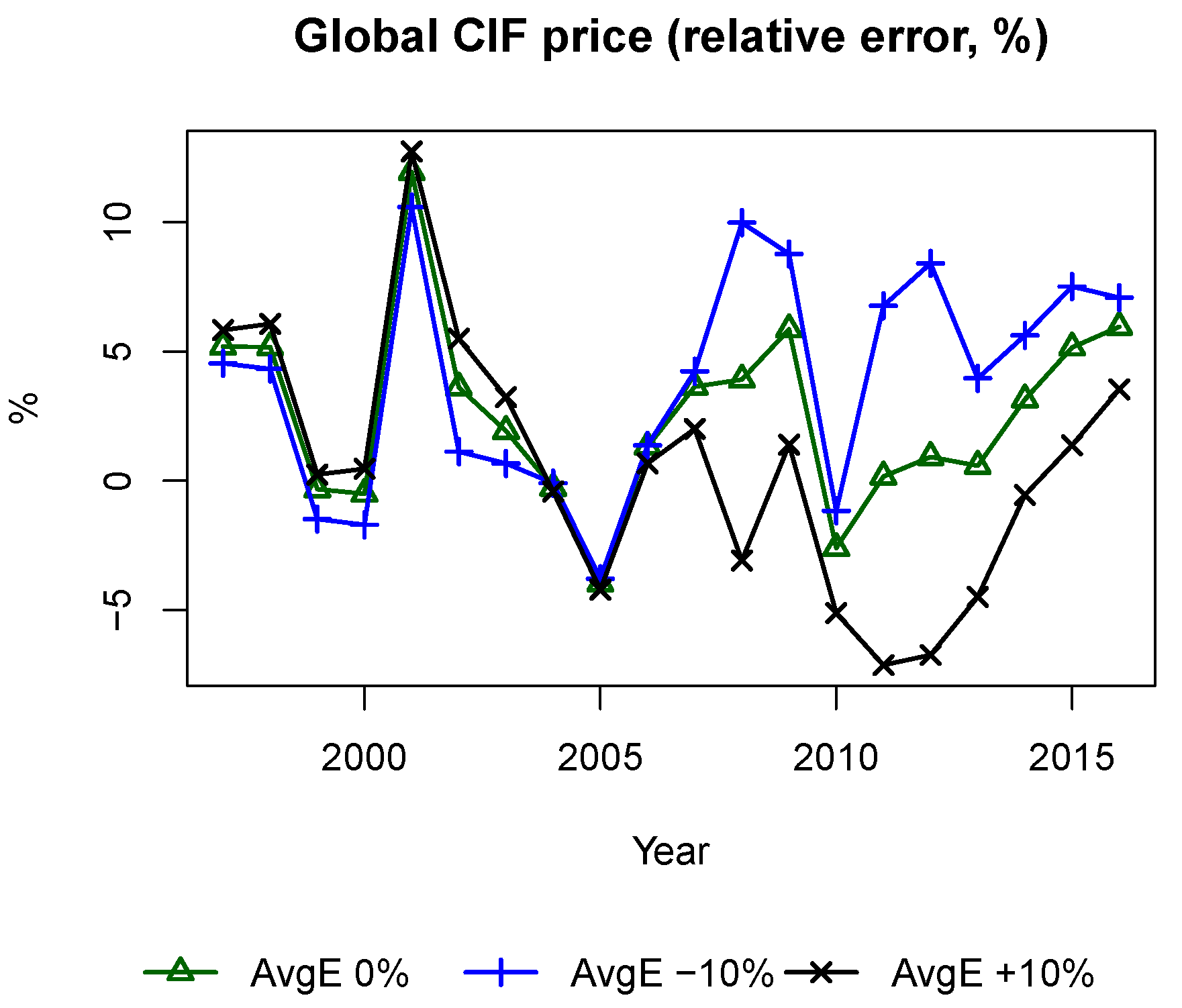
Figure 9.
Relative error in estimating global free-on-board (FoB) price by unperturbed model ensemble “AvgE 0%”; an ensemble with supply curves shifted by -10% (demand curves lifted by 10%), “AvgE-10%”; and an ensemble with supply curves shifted by +10% (demand curves lowered by 10%), “AvgE+10%”.
Figure 9.
Relative error in estimating global free-on-board (FoB) price by unperturbed model ensemble “AvgE 0%”; an ensemble with supply curves shifted by -10% (demand curves lifted by 10%), “AvgE-10%”; and an ensemble with supply curves shifted by +10% (demand curves lowered by 10%), “AvgE+10%”.
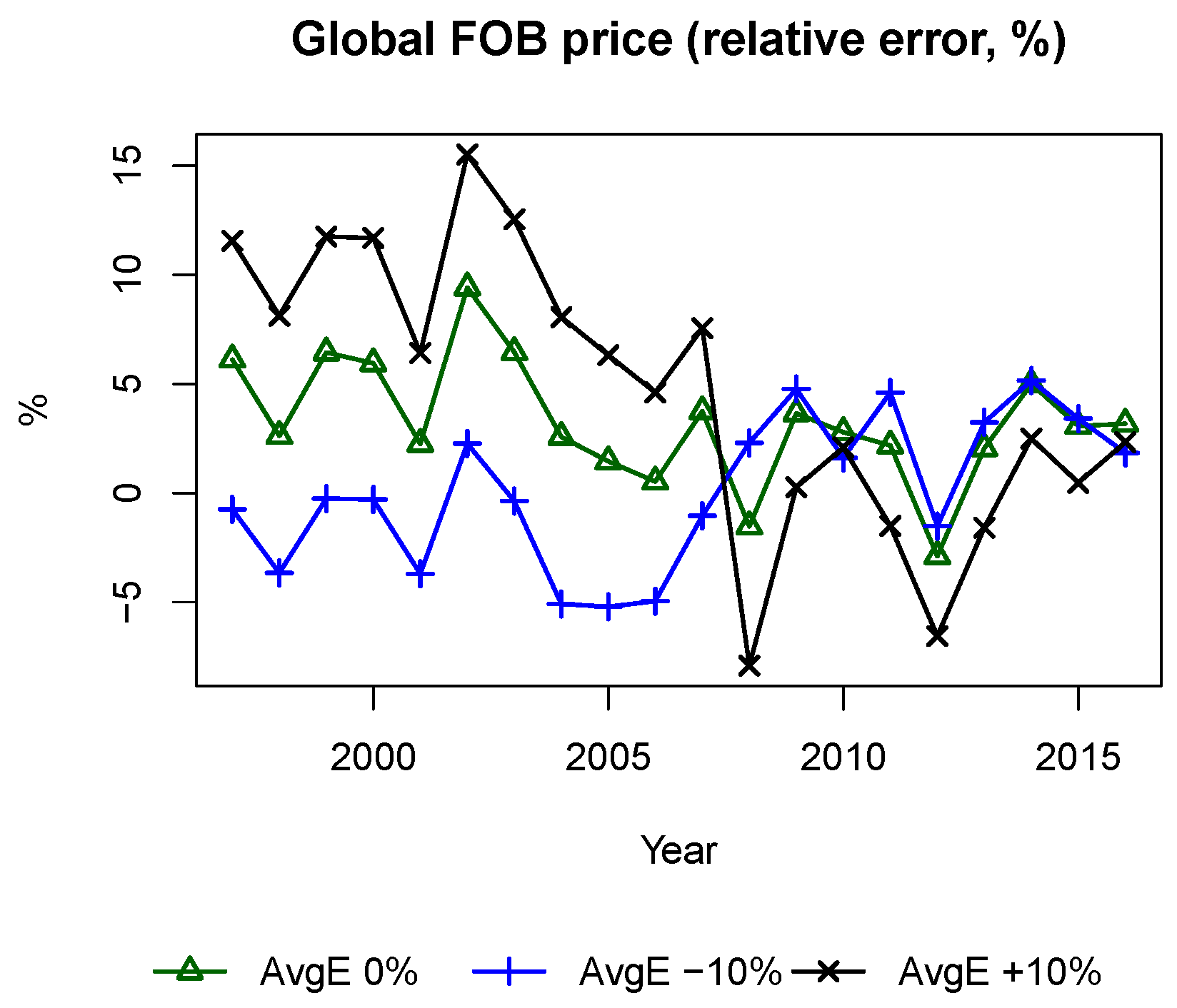
Figure 10.
Relative error in estimating global phosphate rock (PR) traded quantity by unperturbed model ensemble “AvgE 0%”; an ensemble with supply curves shifted by −10% (demand curves lifted by 10%), “AvgE-10%”; and an ensemble with supply curves shifted by +10% (demand curves lowered by 10%), “AvgE+10%”.

Figure 11.
Estimation of global phosphate rock (PR) traded quantity by unperturbed model ensemble “AvgE 0%”; an ensemble with supply curves shifted by −10% (demand curves lifted by 10%), “AvgE-10%”; an ensemble with supply curves shifted by +10% (demand curves lowered by 10%), “AvgE+10%”; and values reported in the United Nations (UN) Comtrade database, “Rep”.

Table 1.
Detailed correction statistics at the final stage of data harmonization—shares of different correction types, using plausible values of cost, insurance, and freight (CIF) and/or free-on-board (FoB) prices, removed records, and respective shares of corrected records and volume.
Table 1.
Detailed correction statistics at the final stage of data harmonization—shares of different correction types, using plausible values of cost, insurance, and freight (CIF) and/or free-on-board (FoB) prices, removed records, and respective shares of corrected records and volume.
| Correction Based on | Records | Volume |
|---|---|---|
| CIF & FoB | 39.1% | 54.3% |
| CIF only | 45.0% | 23.4% |
| FoB only | 14.9% | 16.8% |
| Removed | 0.9% | 5.5% |
Table 2.
Mean absolute errors (MAEs) in traded phosphate rock (PR) quantity estimation for exporters. Minimums, averages, and maximums are taken over the years 1997–2016. “Avg97-16” provides estimates by using a constant per-country average over the period; “AvgEns Naive” and “AvgEns LP” are respectively naive and optimization-based ensemble averages.
| Min | Avg | Max | |
|---|---|---|---|
| 20 | 33 | 61 | Avg97-16 |
| 23 | 34 | 57 | AvgEns Naive |
| 8 | 13 | 25 | AvgEns LP |
Table 3.
Mean absolute errors (MAEs) in traded phosphate rock (PR) quantity estimation for importers. Minimums, averages, and maximums are taken over the years 1997–2016. “Avg97-16” provides estimates by using a constant per-country average over the period; “AvgEns Naive” and “AvgEns LP” are respectively naive and optimization-based ensemble averages.
| Min | Avg | Max | |
|---|---|---|---|
| 13 | 33 | 62 | Avg97-16 |
| 17 | 35 | 58 | AvgEns Naive |
| 7 | 15 | 40 | AvgEns LP |
© 2018 by the authors. Licensee MDPI, Basel, Switzerland. This article is an open access article distributed under the terms and conditions of the Creative Commons Attribution (CC BY) license (http://creativecommons.org/licenses/by/4.0/).
Share and Cite
MDPI and ACS Style
Khabarov, N.; Obersteiner, M. Modeling Global Trade in Phosphate Rock within a Partial Equilibrium Framework. Sustainability 2018, 10, 1550. https://doi.org/10.3390/su10051550
AMA Style
Khabarov N, Obersteiner M. Modeling Global Trade in Phosphate Rock within a Partial Equilibrium Framework. Sustainability. 2018; 10(5):1550. https://doi.org/10.3390/su10051550
Chicago/Turabian StyleKhabarov, Nikolay, and Michael Obersteiner. 2018. "Modeling Global Trade in Phosphate Rock within a Partial Equilibrium Framework" Sustainability 10, no. 5: 1550. https://doi.org/10.3390/su10051550
Note that from the first issue of 2016, this journal uses article numbers instead of page numbers. See further details here.