The Economic Effect of Virtual Warehouse-Based Inventory Information Sharing for Sustainable Supplier Management


1
Asia Pacific School of Logistics, Inha University, 100 Inharo, Nam-Gu, Incheon 22212, Korea
2
Business school, Kwangwoon University, 26 Kwonagwoon-gil, Nowon-Gu, Seoul 139-701, Korea
*
Author to whom correspondence should be addressed.
Sustainability 2018, 10(5), 1547; https://doi.org/10.3390/su10051547
Submission received: 22 January 2018
/
Revised: 8 May 2018
/
Accepted: 8 May 2018
/
Published: 13 May 2018
(This article belongs to the Special Issue Toward Sustainability: Supply Chain Collaboration and Governance)
Abstract
:With the rapid development of information and communication technologies, inventory information sharing between a manufacturer and its suppliers is becoming easier than ever. In line with this trend, we focus on the virtual warehouse where only inventory information on all of the material provided by the suppliers can be stored and shared. Unlike traditional supplier management, the manufacturer constructs and operates this virtual warehouse to check the inventory levels of all the required material at the same time, but each supplier can access only the information about its inventory. This virtual warehouse-based approach can foster a tight relationship between the manufacturer and its suppliers and can handle suppliers as a single company without a large investment in constructing a physical warehouse. The virtual warehouse-based approach seems to be more economically sustainable. To investigate the effect of inventory information sharing via the virtual warehouse, we developed and analyzed a system dynamics-based simulation model. The experiment results show that sharing the inventory information of the suppliers via the virtual warehouse can help manufacturers to achieve better operational performance on several important measures, such as the reduction of finished goods inventory, parts purchasing quantity, degree of backlogs, and total cost.
1. Introduction
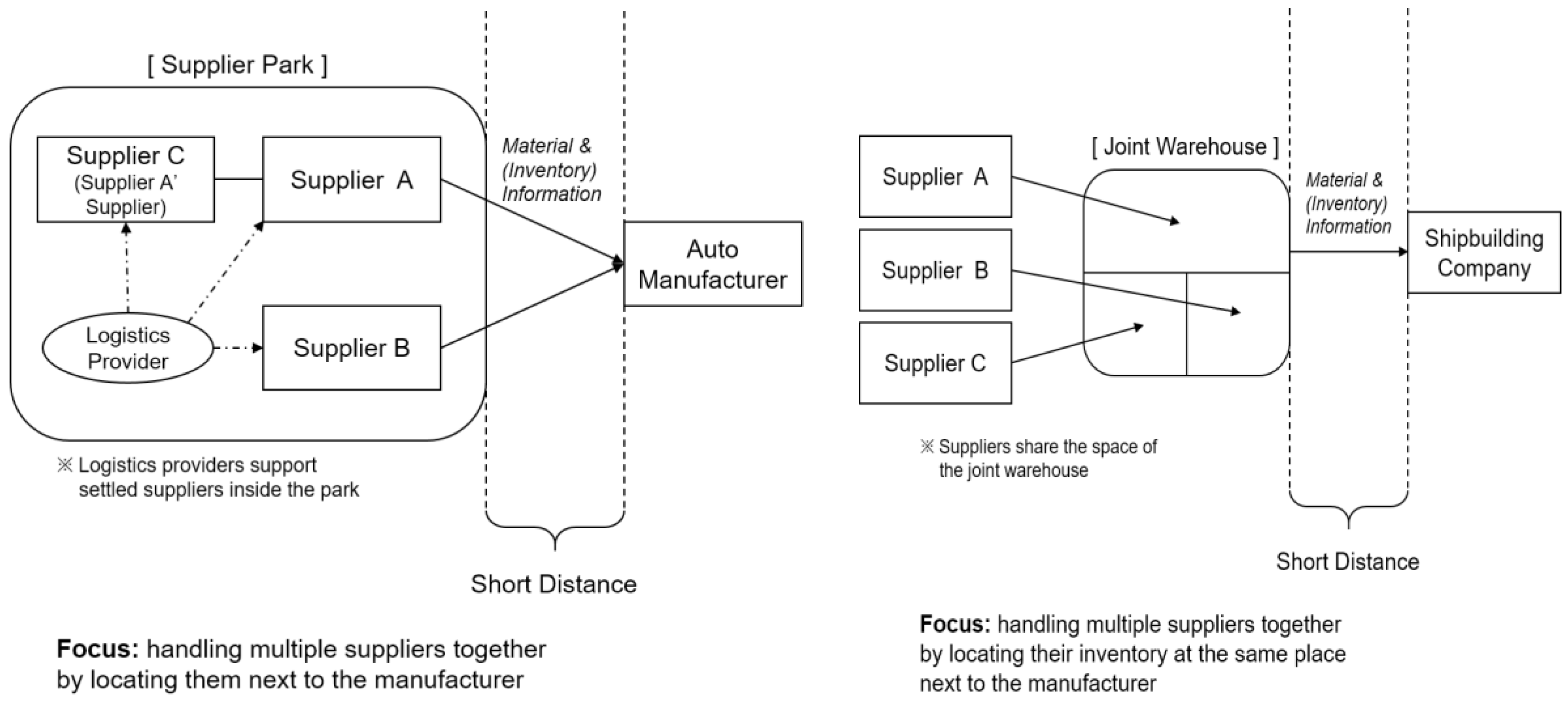
Recent developments in information and communication technologies have facilitated collaboration among business partners, such as manufacturers and suppliers. Firms have begun considering how real-time information sharing among business partners can provide benefits to both a manufacturer and its suppliers [1]. Focusing on purchasing and inventory management, manufacturers want to purchase the correct amount of material from their suppliers on time, which can lead to a reduction in total purchasing and inventory carrying costs. Additionally, suppliers have an interest in maintaining a proper level of material inventory to support their customers (i.e., manufacturers). In the past, it was difficult for both a manufacturer and its suppliers to share information in real-time due to high investment costs or a lack of related technologies. However, with the rapid development of information and communication technologies, some industries are trying to devise an inventory information sharing mechanism between a manufacturer and its suppliers to better manage the material flow from the suppliers to the manufacturer. In the German automotive industry, the concept of the supplier park is well established to increase the delivery service level, cost savings, and development of relationships between the auto manufacturer and its suppliers for just-in-time procurement [2]. This supply park was formed by a German auto manufacturer and consists of the nodes in the supply chain from the sub-supplier to the auto manufacturer, next to the auto manufacturer’s plant [3]. By sharing information about the auto manufacturer’s requirements, the suppliers provide the necessary components on demand. Another example of inventory information sharing between the manufacturer and its suppliers can be found in the Korean shipbuilding industry. Company K, a Korean shipbuilding company, has many suppliers that provide various components and parts, such as pipes, machinery, engine parts, design elements, and electric-electronic parts. Company K established a joint warehouse of components and parts for its suppliers and assigned warehouse space to store the materials delivered by each supplier. After the establishment of this joint warehouse, suppliers save on warehouse operating costs because they do not need to operate their own warehouse, and Company K removed all of the direct delivery routes from many suppliers, which increased complexity. Instead, Company K is concerned only with the delivery route between the joint warehouse and its shipbuilding sites by checking the level of the material inventory in the joint warehouse. Figure 1 briefly describes two industrial cases: the supplier park and the joint warehouse.
As seen in the above industrial cases, a park or a joint warehouse where multiple suppliers join and share plays an important role in fostering a relationship between a manufacturer and its suppliers. If the manufacturer can handle its multiple suppliers as one company from the viewpoint of inventory and delivery management, it benefits from reductions in both related costs and complexity. Additionally, the on-time delivery of the required material from various suppliers via the joint warehouse can be easily achieved when needed.
However, the above industrial cases focused on the physical aspect of grouping the suppliers. Manufacturers need to invest large sums of money in constructing and operating a supplier park or a joint warehouse for their suppliers. Thus, this type of supplier management seems to be economically unsustainable for the manufacturer. Although suppliers that provide material to the same manufacturer can build a joint warehouse, it is difficult for those suppliers that have different buyers (manufacturers) to collaborate with each other by spending their investment costs. Thus, the above cases also seem to be economically unsustainable to the suppliers.
Thus, in this research, we focus on the virtual warehouse (VW), where inventory information on the materials provided by the suppliers can be stored together. The manufacturer constructs and operates this VW to check all of the inventory levels of the required material at the same time, and each supplier can access (record or update) the information about its inventory. By adopting this VW, both the manufacturer and the suppliers are expected to derive similar benefits from the supplier park or the joint warehouse without a large investment in constructing a physical warehouse. Unlike the existing supplier management, such as a supplier park or joint warehouse, this VW-based supplier management is realistic and sustainable. Additionally, with the help of the rapidly developing communication technologies, the VW-based sustainable supplier management will receive more attention from real world. The concept of the VW in this research is depicted as shown in Figure 2.
This paper stresses the effect of inventory information sharing via a VW between a manufacturer and its suppliers. To investigate how this VW can affect the performance of the manufacturer, such as its finished goods inventory and degree of backlogs, we developed a simulation model and validated the model using a real-world case adopted from a U.S. household electric appliance company (Company H). Among the various techniques for building a simulation model, the authors chose system dynamics (SD) because it is widely known that SD can be used to build system models identifying a robust structure that can accommodate the dynamics of manufacturing or supply chains [4,5,6].
This paper is organized as follows. Related research is presented in Section 2, and a case study using the SD model is discussed in Section 3. In Section 4, the simulation results of the case study are summarized and analyzed. Finally, Section 5 suggests future research directions and gives concluding remarks.
2. Literature Survey
Recent publications regarding our research can be categorized into the following three areas: (1) sustainable supplier management through manufacturer-supplier partnerships; (2) VW; and (3) SD-based simulation. The first two areas are related to our research subject, and the final one is related to the methodology of our research.
2.1. Sustainable Supplier Management through Manufacturer-Supplier Partnerships
The effective implementation of sustainable supplier management through manufacturer-supplier partnerships (MSPs) has been one of the critical issues in achieving successful supply chain management (SCM). Both the manufacturer and the supplier aim to leverage a strategic relationship to gain a competitive advantage. Many recent studies have focused on the importance of the MSP. The term ‘partnership’ stemmed from the collaborative associations forged between assemblers and suppliers in the Japanese automotive industry in the 1960s and 1970s and was used only recently in the West [7]. However, in many studies, partnership is often ambiguous and has been described in different ways from strategic perspectives [8]. Some research focused on the partnership for new product development [9,10,11], while others tried to identify the benefits of such a partnership using various interviews and case studies [12,13]. Additionally, vendor-managed inventory (VMI), another interesting collaboration between a manufacturer and a supplier, has been initiated to reduce inventory costs and to increase fill rates [14]. In VMI, by using the inventory information received from the buyer, suppliers can plan their production runs, schedule deliveries, and manage the order volumes and inventory levels at the buyer’s stock-keeping facilities. VMI integrates operations between suppliers and buyers (i.e., manufacturers or retailers) through information sharing and business process reengineering, and many applications of VMI can be found in related research [15,16,17,18,19].
Since a firm’s supplier performance has a significant impact on many of its product dimensions, such as cost, quality, and on-time delivery [20], manufacturers have an interest in building a good partnership with their suppliers.
Although there are various past studies regarding the MSP, most of them have focused on specific processes, such as new product development or quality issues. Additionally, for inventory management, past research addressed VMI as the MSP. Thus, there is a lack of research on inventory information sharing between a manufacturer and its suppliers via a (manufacturer-driven) VW shared by the suppliers.
2.2. Virtual Warehouse
VW is a business model that aims to reduce costs, optimize production and provide high-quality customer service among supply chain channels [21]. Additionally, the VW is dependent on information technologies and real-time decision algorithms to provide operating efficiencies and global inventory visibility comparable to those achieved in a single-location, world-class warehouse [21]. Most previous research considered a VW operated by the manufacturer, focusing on the distribution between the manufacturer and customer for better customer service [21,22]. The frequent changes in customer orders led to an insufficient inventory, which meant that the available inventory at the manufacturing site was lower than the customer demand. VW can resolve this situation using inventory relocation, which assigns inventory at different or remote manufacturing sites to the given customer demand. This action can only be undertaken in VW, which means that inventory relocation is conducted using inventory information instead of physical stock movement. Thus, the inventory at different or remote manufacturing sites is tagged for its final customer (i.e., destination) in the VW. Landers et al. [22] proposed a VW model for the field repair service of a business telephone system. Using the VW model, they argued that the productivity and utilization of skilled field technicians were improved. Fung et al. [21] presented a VW system that is capable of refining inventory planning to streamline product planning and control if there is an abrupt change in the product demand. Their VW system was designed for the manufacturer to handle its own inventory to cope with the demand change without incorporating the supplier into the design of the VW. Other researchers viewed the VW as an inventory pooling or inventory consolidation technique [23,24]. The idea is that inventory increases as the standard deviation of either demand or lead time increases. Companies may attempt to reduce inherent variation using pooling [25]. Inventory pooling refers to a complex system in which different stocking points, either from intra-operational or inter-operational organizations, share their inventories with the aim of reducing costs while improving the overall performance in terms of both logistics and maintenance management [26]. Yang and Ma [27] proposed the VW-based inventory management of the spare parts under emergency. In their research, the VW was utilized to manage the inventory of the various spare parts stored in multiple sites together in order to cope with emergencies (i.e., unexpected demand surge, etc.). More recently, Mathien and Suresh [28] investigated the appropriate supply chain structures for implementing the VW via information sharing among the manufacturer and retailers.
The VW is an appropriate tool for inventory-pooling because it provides a powerful search engine that helps check all inventories at multiple sites and locates the abrupt demand or order to any site online.
As summarized above, although many researchers have studied VWs, they considered only a single manufacturer and its product distribution network composed of multiple physical warehouses. Additionally, most of the existing research on VW focused on the design architecture of a VW system without analyzing the performance using simulation models. Additionally, a VW shared by multiple suppliers who provide material to the same manufacturer (buyer) has not been explored.
2.3. System Dynamics-Based Simulation
To analyze the various dynamics occurring in a supply chain, computer simulations are widely used and considered an effective method. Additionally, queuing theory plays a very important role and sets the framework for these simulations because capturing the interactions between demands and backlogs is a critical factor in any supply chain. Ballou [29] indicated that when more than two echelons are involved, managing the inventory throughout the supply chain becomes too complex for mathematical analysis and is usually performed with the aid of computer simulation.
For computer simulation models, discrete-event simulation (DES) and SD are two widely-used modelling tools [30,31,32]. Although both of them are built to understand how systems behave over time, some technical differences exist between the modelling approaches in terms of their underlying principles [33]. For example, DES models systems as network queues and activities where state changes occur at discrete points in time, whereas SD models represent a system as a set of stocks and flows where the state changes occur continuously over time [34]. Additionally, considering the nature of the problem modelled, SD focuses on strategic issues and policy analysis, while DES is used to analyze problems at an operational or tactical level [35]. A brief comparison of DES and SD using the previous related literature [34,35] is summarized as shown in Table 1.
Tako and Robinson [32] investigated the application of both DES and SD in the logistics and supply chain context, and they classified the issues in the supply chain into either the strategic/policy or operational/tactical group. According to their classification, information sharing and supply chain structure issues can be considered strategic/policy issues. Despite technical differences, both simulation approaches can be applied to strategic/policy issues in the supply chain. However, in this research, we chose the SD as the main simulation modelling tool due to its ease of applicability and its fitness for strategic (or policy)-related issues, such as the adoption of VW for information sharing among vendors.
Since Forrester [36] built an SD model of a three-echelon production distribution system and demonstrated how market demands are amplified through transactions in the supply chain, many researchers have adopted the SD model to analyze the various supply chain dynamics [37,38,39]. Recently, Feng [40] showed the importance of information sharing in the supply chain by establishing an SD model of supply chain information sharing and analyzing several scenarios. Costantino et al. (2014) investigated the interaction of collaboration and coordination in a four-echelon supply chain in different scenarios of information sharing levels [41]. This research showed the bullwhip effect and how the inventory variance increased and amplified when a periodic review order-up-to level policy was applied, noting that more benefits were generated when coordination started at downstream echelons. More recently, Cannella et al. [42], by applying the SD model, quantified the impact of inventory record inaccuracy on the dynamics of collaborative supply chains in terms of both operational performance (i.e., order and inventory stability) and customer service level.
As shown above, many studies focused on the MSP, joint warehouse operations, and system dynamics in the supply chain. However, the manufacturer-driven VW for information sharing with multiple suppliers has not been investigated in depth. This paper analyzes the importance of inventory information sharing via the VW using the SD-based simulation. Additionally, to show the feasibility of the simulation, we adopt a real-world case of a U.S. server manufacturer. In the following sections, the real-world case, simulation model, and analysis results are provided.
3. Case Study
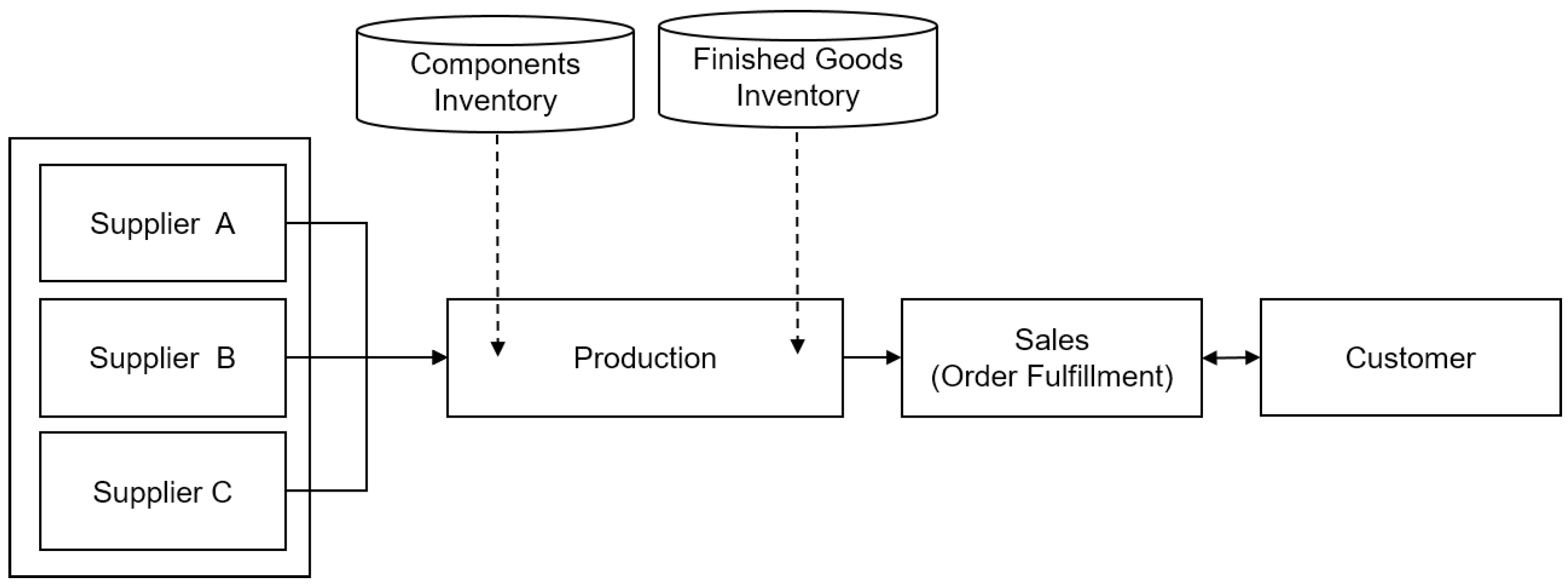
3.1. The Supply Chain Flow of Company H
In this study, we analyzed the effects of information sharing using VW between a single manufacturer and multiple suppliers for the successful achievement of sustainable supplier management. To design a model and investigate the effects of sustainability between the manufacturer and suppliers via VW, we conducted a case study of Company H, a U.S. household electric appliance company. Company H currently manufactures and sells various products, including computers, communication systems, and sound or image media. From the products of Company H, we chose a computer server as the target product for our case study. The supply chain of Company H consists of five entities: the supplier, purchasing, production, sales, and customers. The supply chain flow is triggered by customer orders. When customer orders occur, the sales component manages the order receipts and the proceeds from the customers. This company does not have an agency. The data for demand forecasts are collected in the sales input at SAP (the ERP package), and product orders occur. The product part of the company confirms the quantity of the components needed to produce the number of products received from the sales component and begins to produce the quantity confirmed after the delivery of the components from a warehouse. The purchasing entity determines the purchase quantity though data that are transmitted and order components every 30 days. All of the finished goods are moved into a factory warehouse and transported to customers through the sales component. Company H adopts the make-to-order method and stores raw material and components in a production factory. Figure 3 summarizes the supply chain flow of Company H.
3.2. Causal Diagram
According to Radzicki and Sterman [43], the progressive development of “dynamic” models is preceded by an initial qualitative phase of the formalization of the causal relations in the systems, starting from our preliminary investigation. The structure of any system can be exhibited by a causal loop diagram [44]. It captures the major feedback mechanism and shows the variables and their interactions, where arrows indicate the cause (the arrow’s origin) and its direct effect (the arrow’s point). According to the well-known causal links representations, these arrows are indexed and show how they influence variables. A minus sign (−) means that a change in a variable’s value consequently induces a change in the destination variable in the opposite direction. Conversely, a plus sign (+) means that the two correlated variables are directed in the same way. Figure 4 shows the causal diagram that describes the flow of data and material for the supply chain of Company H. This study focuses on the implementation of five objects and their activated logics that consist of the supply chain of Company H: suppliers, purchasing, production, sales, and the customer.
3.3. Modeling of the System Structure
System dynamics is a method for managing a complex systemic problem with a combination of quantitative and qualitative methods based on feedback control theory. In simulation modeling, the “level” or “stock” variables describe the state of the systems by the continuous integration of the actions resulting from these systems, and the “flow” variables express actions. The levels exist permanently. If any activity were to cease, the flows would disappear. This mode of representation makes it possible to represent the variations of these states through differential equations and to study their dynamic behavior. Additionally, “rate” represents any decision that can change the inventory level, which is influenced by the flow, such as product warehousing and delivery. “Auxiliary” is a “need variable” to describe “level”, “rate”, and “other auxiliaries”. This progressive modelling leads us to continuous simulations, which allow us to visualize stabilized behaviors and to analyze characteristic phenomena of instability within certain real systems. Vensim, which can embody system dynamics, was used to construct a supply chain causal diagram for Company H. Vensim is the software developed by Ventana Systems Inc. (Massachusetts, USA) for systems dynamics model development.
This simulation model was divided into five parts: the sales part, the production part, the sales loss handling part, the purchase part, and the supplier (A, B, and C) parts. This study constructed two types of models, the case that considers the inventory sharing system and the case that does not do so, to understand the effect of the inventory sharing system when comparing the two models. Therefore, we made two models: the case in which suppliers A, B, and C have an inventory warehouse and the case in which suppliers A, B, and C have a VW that integrates and shares component inventories from all of the suppliers. The Appendix supplements the simulation structure and modelling by providing the equations for calculating the variables used in each part, such as sales logic (Appendix A), production logic (Appendix B), and purchasing logic (Appendix C).
Company H must make forecasts far in advance because its response time (the time between the moment when the customer places his/her order and the date on which the ordered product is received) is shorter than its cumulative production cycle. The firm must launch the production of goods on the basis of a forecast of its future sales. These forecasts are characterized by a very remote horizon, which explains the considerable uncertainty of their effectiveness (the chances of overstocking or encountering shortages increase).
3.4. The Case with No Inventory Sharing System (without VW)
This model depicts the situation in which suppliers A, B, and C have inventory warehouses, as shown in Figure 5. Each supplier receives orders, produces parts, and sells parts without any information sharing. The parts inventory is increased by the parts production and is decreased by parts sales. Parts production increases the parts inventory. Parts inventory is decreased by parts sales. The target production of parts is controlled by parts inventory adjustment and parts sales. Parts inventory adjustment is decided by the gap between the target inventory and the parts inventory. The parts inventory holding cost is allotted as 10 for every increase of 100 units. The parts transportation cost is calculated by multiplying the transportation frequency and the cost of transport per unit. The parts relevant cost is determined by the parts inventory holding cost, parts transportation cost, and the parts price. The parts price is a low numerical value because the comparison of the assumptive total cost is an indirect comparison. Each order rate of the suppliers A, B, and C is 4:3:3. In figure 5, “++a day” means an increase of one day during the simulations
- “Parts order” = “Parts purchase quantity” × (4/10)
- “Parts target production” = “Parts sales” + “Parts inventory adjustment”
- “Parts production” = “Parts target production”
- “Parts target inventory” = “Parts sales” × 0.15
- “Parts production” = “Parts target production”
- “Parts transportation capacity” = 100
- “Parts transportation cost per unit” = 500
- “Parts sales” = “Parts order”
- “Parts inventory” = INTEG (Parts production - Parts sales, 0)
- “Parts inventory adjustment” = Parts target inventory - Parts inventory
- “Parts inventory holding cost” = Parts inventory holding cost lookup (Parts inventory)
- “Parts inventory holding cost lookup (((0,0) − (300,30)), (0,0), (100,10), (200,20), (300,30))
- “Parts transportation cost” = Roundup (“Parts purchase quantity/”Parts transportation capacity, 0) × Part transportation cost per unit
3.5. The Case with Inventory Sharing System (With Virtual Warehouse)
This model depicts the situation in which suppliers A, B, and C virtually have an inventory sharing warehouse. Therefore, information on all of the parts produced by suppliers A, B, and C is shared in a Virtual based (VB), and the sales for suppliers A, B, and C are conducted using the information in the VB. A numerical formula is the same as the prior model, except for the VB part, as shown in Figure 6. The calculation of VB transportation cost is the same as case with no information sharing.
- “VB parts production cost” = VB parts inventory holding cost + 2
- “VB parts price” = “VB parts production cost” + 2
- “VB parts inventory holding cost” = VB inventory holding cost lookup (((0,0) − (300,30)), (0,0), (100,10), (200,20), (300,30))
- “VB transportation capacity” = 100
- “Parts transportation cost per unit” = 500
- “VB transportation cost” = Roundup (“VB Parts purchase quantity/”VB Parts transportation capacity, 0) × VB Part transportation cost per unit
- “Virtual warehouse” = INTEGRAL ((A parts production + B parts production + C parts production) − (A parts sales + B parts sales + C parts sales), 0)
4. Experimental Results
4.1. Verification of Simulation
With the appropriate settings for the term of the simulation (i.e., 365 days) and the parts order cycle (i.e., 30 days), the running results of the developed simulation model seemed to be very similar to the real data (Figure 7) of Company H for the recent year.
The purchase parts and holding parts inventory quantities also had similar values. However, the finished goods inventory had a higher value than the real data. Overall, the pattern shape of the graph was similar to the real data. Therefore, the simulation model in this study reflects the reality of the Company H supply chain.
4.2. The Effect of Virtual Warehouse Practices for Sustainable Supplier Management
As noted earlier, information sharing via a VW is an effective method for successfully achieving a sustainable manufacturer-supplier relationship. To see the effect of sustainability, a “what if” analysis was conducted to contrast the two different cases of whether an inventory sharing system was constructed or not.
As shown in Figure 8, the finished goods quantity of the case that considered the inventory sharing system was smaller than the case that did not consider the inventory sharing system. Additionally, the graph had a more stable shape.
The discrepancy between the case that considered the inventory sharing system and the case that did not consider the inventory sharing system was 5699, as shown in Table 2. This result means that the inventory sharing system reduced the inventory quantity of finished goods by approximately 30%.
The parts purchase quantity of the case that considered the inventory sharing system was smaller than the case that did not consider the inventory sharing system.
The discrepancy between the case that considered the inventory sharing system and the case that did not was 5,606,955 parts, as shown in Table 2. This result means that the inventory sharing system reduced the parts purchase quantity by approximately 10%. Therefore, the parts inventory holding cost decreased.
The degree of unattended orders (backlog) of the case that considered the inventory sharing system was smaller than the case that did not. The result is that customer satisfaction increased because of the decrease in unattended orders.
The discrepancy between the case that considered the inventory sharing system and the case that did not was 5561, as shown in Table 2. This result means that the inventory sharing system reduced the unattended order rate by approximately 7%. Therefore, the sales loss decreased.
Transportation cost in the case of information sharing was decreased by about 26.3%, compared to the case with no information sharing, as shown in Table 2.
This assumptive cost was considered to not evaluate the correct cost of all of the supply chain but instead to analyze the effects of important variables (finished goods, parts inventory, sales loss, order cost, parts transportation cost, and parts relation cost) related to the cost of information sharing.
As shown in Table 2, the accumulated total cost of the case that considered the inventory sharing system was smaller than that of the case that did not. As a result, the effect of the inventory sharing system was reflected in various cost relation parts, such as the inventory and sales loss.
The discrepancy between the case that considered the inventory sharing system and the case that did not was 53,808 parts per day, as shown in Table 2.
This result means that the inventory sharing system can reduce the total cost rate by approximately 11.3%. Therefore, the total cost is decreased in the case of the inventory sharing system.
4.3. The Contrast of Order Cycle (30 Days, 14 Days, and 7 Days)
The assumption of this analysis was that the more frequently that the parts were ordered in Company H, the less the charge of the inventory was; this effect was sufficient to offset the increase in the order cost as a result of the increased frequency of parts orders. Therefore, this research assumed that the total cost in the supply chain decreased. In this part, only the case that considered the inventory sharing system was simulated and evaluated by the changing order cycle because this model had better results than did the case that did not consider the inventory sharing system. The length of the cycle was established as 30 days, 14 days, and 7 days, and the length of the cycle was changed by a cycle lookup. The comparison variable (finished goods, parts inventory, sales loss, order cost, and parts relation cost) was established to analyze the effect of the supply chain from the cycle change. Decreasing the cycle of parts orders means that the frequency of parts orders increased with an increase in the order cost. Therefore, the more the cycle of parts orders decreased, the lower the order quantity per order became, but the total order cost increased, as shown in Table 3.
Table 3 also shows that the reduction of the order cycle decreased the purchase quantity per order under the same conditions.
The parts inventory in the supply chain was considered an important variable to show how the parts inventory changed with a decrease of the average parts purchase quantity per order.
The average parts inventory quantity in the case of the 14-day order cycle was much smaller than the case of the 30-day order cycle. However, the discrepancy between 14 days and seven days was low. The discrepancy of the finished goods inventory caused by the order cycle change was low, and the finished goods inventory was the lowest at seven days, as shown in Table 3.
The assumptive total cost was considered, not to evaluate the correct cost of the entire supply chain, but to analyze the effect of the important variables (finished goods, parts inventory, sales loss, order cost, and parts relation cost) related to the cost by information sharing. The more frequent the parts orders became, the more the assumptive total cost increased. This scenario implies that an increase in the parts order frequency reduced the cost of the supply chain because the finished goods inventory, parts inventory quantity, and average parts purchase quantity per order were decreased by the increase in the order frequency. Sales losses caused by the non-fulfilment of the order handling term decreased as the order cycle was reduced.
4.4. Findings and Implications
The finished goods quantity and the parts purchase quantity of the case that considered the inventory sharing system was smaller than those of the case that did not consider the inventory sharing system, and the graph shape was more stable.
The degree of the unattended order (backlog) of the case that considered the inventory sharing system was smaller than the degree of the case that did not. This scenario implies that customer satisfaction increased because the unattended orders decreased. The lost sales also decreased.
The assumptive total cost of the case that considered the inventory sharing system was smaller than that of the case that did not consider the inventory sharing system. This scenario means that the effect of the inventory sharing system was reflected in various cost relation parts, such as inventory and sales losses.
A reduction of the parts order cycle or an increase in the order frequency decreased the parts purchase quantity per order, but the order cost increased. A reduced parts purchase quantity reduced the holding inventory quantity.
As the frequency of the parts orders increased, the assumptive total cost also increased. This scenario implies that the increase in the parts order frequency reduced the cost of the supply chain because the finished goods inventory, parts inventory quantity, and average parts purchase quantity per order decreased with an increase in order frequency.
With respect to the result for the assumptive total cost, considering all of the variables, the assumptive total cost was the smallest at the seven-day order cycle, but the total costs of the 14-day case and the seven-day case were similar. As a result, the increase in the order frequency increased the order cost.
This research not only highlighted the value of information sharing by checking the specific economic benefits for the manufacturer, but also suggested a new possibility of vendors’ collaboration among themselves. Joint pick-up and transport via milk-runs can be adopted to save the time and money of the vendors. Figure 9 shows an example of the joint pick-up and transport among vendors. As shown in Figure 9, if suppliers are located relatively close to each other, and they pursue a joint pick-up and transport of parts/components which should be delivered to the manufacturer, the proposed VW based approach might be better applied.
In addition, if vendors need not consider inventory management, including how much holding and transporting, they could focus on the quality of material and save their efforts. The manufacturer could increase the accuracy of the in-bound logistics plan of materials (which leads to the economic benefits) by constructing and controlling the VW. In short, both the manufacturer and its vendors could obtain benefits from the VW in terms of quantitative (e.g., time, cost, etc.) and qualitative (e.g., fostering collaboration in supply chains, increasing the accuracy of plan/schedule) aspects.
In short, the VW is an appropriate tool for inventory-pooling by the manufacturer who monitors suppliers’ inventory levels and aggregates them in virtual environments on a real-time basis. Unlike the vendor-managed inventory (VMI), the VW of this paper enables the manufacturer to be responsible for controlling suppliers’ inventory located at various sites.
4.5. Generalization of the Proposed Simulation Model
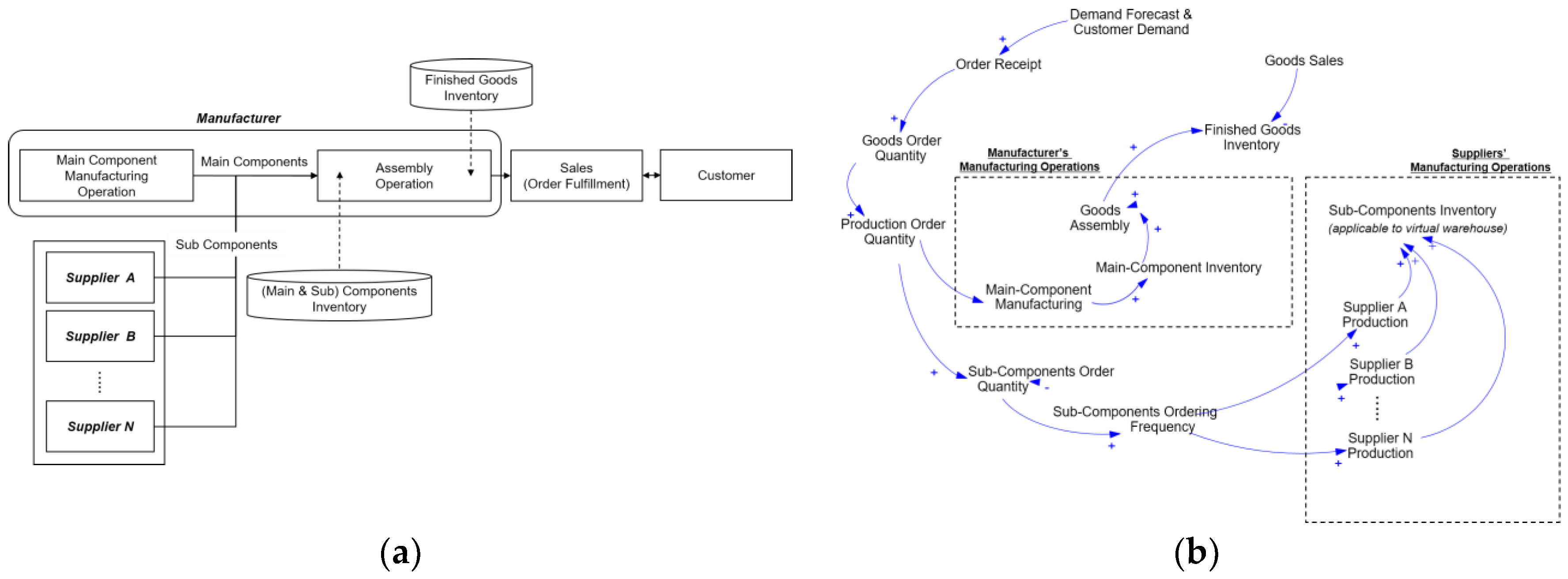
The proposed simulation model can be used for other supply chains where any manufacturer has an assembly operation and multiple suppliers. Many manufacturers have the assembly operation to produce final products (e.g., the household electric appliance of company H), and the inputs of the assembly operation (i.e., the material or semi-finished products) are from either the former operations inside of the factory or the outside suppliers. For example, a thin-film transistor liquid crystal display (TFT-LCD) manufacturing process has a similar structure based on the assembly operation. The TFT-LCD manufacturing process has three basic stages: thin-film transistor (TFT) fabrication, liquid crystal (LC) assembly, and the module assembly process. The module assembly process is the last stage of TFT-LCD manufacturing processes, where the TFT-LCD panels passed from the LC assembly process are assembled with the other necessary parts to complete the final TFT-LCD product. The module assembly process requires approximately 16 distinct, essential parts, most of which are provided by external suppliers [45]. The basic supply chain flow of this TFT-LCD manufacturing process is very similar to that of Company H in terms of the relationship between the manufacturer and its suppliers around the assembly operation.
Thus, the proposed simulation model can be applied to any manufacturer’s supply chain that has an assembly operation and suppliers that provide parts or semi-finished products, such as the TFT-LCD manufacturing process, without a significant modification of the proposed simulation model. The generalized supply chain and its corresponding causal diagram can be depicted as shown in Figure 10.
5. Conclusions
In this research, we analyzed the positive and economic effects of sustainable supplier management via a VW between a manufacturer and its suppliers.
A VW where only inventory information on all the material provided by the suppliers can be stored and shared can replace a physical joint warehouse or a supplier park without a large investment. To implement a sustainable relationship with suppliers, the manufacturer designs and operates this VW to check all the inventory levels of the required material at the same time and orders the delivery of any required material when needed. By sharing the inventory information of the suppliers via the VW, the manufacturer can achieve better operational performance on several important measures, such as the reduction of finished goods inventory, parts purchasing quantity, degree of backlogs, and total cost.
There also exist some potential limitations regarding this research: (i) we further need to consider the way to implement the VW model effectively when suppliers are not willing to share their inventory and cost with the manufacturer; (ii) to argue the justification of our proposed model, the strong cases for considering VW where the manufacturer controls the pools of supplier inventory should present; (iii) although the simulation results have been validated using various scenarios which mimic real situations, it was not possible to evaluate the proposed simulation model using the exact data gathered from the real world; (iv) a what-if analysis using the proposed simulation model should follow to check how parameters can affect the performance of the VW; and (v) more scenarios from various supply chain partnerships need to be checked using the proposed simulation model. Although we show some possibilities regarding the generalization of the proposed model, extensive experiments using real data gathered from other supply chains are required.
Additionally, for simplicity, we designed the simulation model by considering only some important costs, such as inventory, ordering, and sales loss costs. For an in-depth discussion of the effects on sustainable supplier management through a VW, our model could be expanded to include a financial component that reflects the real costs, including production cost and profitability, for Company H. Finally, our future research will consider developing the modular components for the simulation model by adding various indicators evaluating all three aspects of sustainability; economic, environmental, and social perspectives between a manufacturer and its suppliers.
Author Contributions
Hosang Jung(First Author) formulates “virtual warehouse” concept and draws up a research framework. Sukjae Jeong(Corresponding Author) designs an experimental plan and summarizes the simulation results.
Acknowledgments
The present research has been conducted by the Research Grant of Kwangwoon University in 2017. This work was supported by the Ministry of Education of the Republic of Korea and the National Research Foundation of Korea (NRF-2017S1A5B8060156).
Conflicts of Interest
The authors declare no conflict of interest.
Appendix A. Variables and Equations Used in Sales Logic
A backlog, a stock variable, is established to accumulate the gap values between the order receipt amount and the quantity of the order completed every 30 days. The order receipt is given by summing up sales forecasts and non-forecast demand. A sales loss variable is established as the process that considers backlog every 30 days. In order to originate a “sale loss” as a “sales loss handing cycle”, variable M is used in this logic.
In the following pseudocodes, the RANDOM UNIFORM (m, x, s) function provides a uniform distribution between m and x (exclusive of the endpoints). RANDOM NORMAL (m, x, h, r, s) provides a normal distribution of mean 0 and variance 1 before it is stretched, shifted, and truncated. This is equivalent to a normal distribution with mean h and standard deviation r. The units of r should match m, x, and h.
Here, m is the minimum value that the function will return. Where necessary, the distributions will be truncated to return values above this. Truncation occurs after the output has been stretched and shifted. If the number drawn is below this value it will be discarded and another number drawn. x is the maximum value that the function will return. Where necessary, the distributions will be truncated to return values below this. Truncation occurs after the output has been stretched and shifted. If the number drawn is greater than this, it will be discarded and another number drawn.
h is a shift parameter that indicates how much the distribution will be shifted to the right after it has been stretched (but before being truncated). r is a stretch parameter that indicates how much the distribution will be stretched before it is shifted and truncated. Note that for the NORMAL distribution h and r correspond to the mean and standard deviation. s is a stream ID for the distribution to use.
- Backlog = INTEG (Order receipt - Order completion, 0)
- Order receipt = Product order
- Order completion = IF THEN ELSE (Sales loss handing = 1, Backlog, Transportation)
- Sales forecast = 23 + sin(RANDOM UNIFORM (6, 6.28, 0))
- Non-forecast demand = RANDOM NORMAL (0, 8, 4, 3, 0)
- Product order = Sales forecast + Non-forecast demand
- Sales loss = IF THEN ELSE (Sales loss handing = 1, Backlog, 0)
- Variable M = INTEG (“++ a day”, 0)
- Sales loss handling cycle = Lookup for sales loss cycle (Variable M)
- Lookup for sales loss cycle = Lookup ([(0,0)-(365,400)], (0,0.5), (29,0.5), (30,30), (31,0.5), (59,0.5), (60,60), (61,0.5), (89,0.5), (90,90), (91,0.5), (119,0.5), (120,120), (121,0.5), (149,0.5), (150,150), (151,0.5), (179,0.5), (180,180), (181,0.5), (209,0.5), (210,210), (211,0.5), (239,0.5), (240,240), (241,0.5), (269,0.5), (270,270), (271,0.5), (299,0.5), (300,300), (301,0.5), (329,0.5), (330,330), (331,0.5), (359,0.5), (360,360), (361,0.5), (364,0.5), (365,365))
Appendix B. Variables and Equations Used in Production Logic
A production capability is determined by the amount of parts inventory and maximum production capacity. A production lead time is established to represent the required time for goods production. An amount of finished goods inventory is calculated by the production amount and transportation that are affected by the lead time, respectively.
The effect of product price represents the clear increase or decrease in the sales quantity periodically by comparing the preceding product price and the present product price. However, the product price is decided to be a low numerical value because the cost comparison of this study does not consider all of the costs, including the parts and goods production costs, inventory costs, sales loss, and so on, but only the costs that are related to inventory, sales losses, and orders.
In the following pseudocodes, the DELAY FIXED function plays a role to control delays in the flow from an input stock (product price) to an output stock (preceding product price). The initial value of the preceding product price is set to zero, and it is replaced with the present product price after one month. In other words, the present product price (i.e., the input variable) is converted into the preceding product price after one month.
- Production capability = IF THEN ELSE (Parts inventory/50) <= Max. Production capability, Parts inventory/50, Max. Production capability)
- Max. Production capability = 80 + RAMP (0.5, 60, 120)
- Finished goods inventory = INTERG (Product production-Transportation, 5)
- Transportation = IF THEN ELSE (Finished goods inventory <= 0, 0, IF THEN ELSE Finished goods inventory >= sales quantity/Transportation lead time, Finished goods inventory/Transportation lead time))
- Transportation lead time = 1.5
- Sales quantity = 22 + (4 × ABS (SIN (RANDOM UNIFORM (0, 3, 3))))
- Product price effect = IF THEN ELSE (Product price < Preceding product price, 1/(Preceding product price - Product price) × (Preceding product price/Product price), (Preceding product price - Product price) × (Preceding product price/Product price))
- Preceding product price = DELAY FIXED (Product price, 1, 0)
- Sales rate = RANDOM UNIFORM (150, 200, 1)
- Price change = 1/(Preceding product price - Product price)
- Price change rate = IF THEN ELSE (Preceding product price = 0, Preceding product price/Product price)
- Product price = Production cost + 5
Appendix C. Variables and Equations Used in Purchasing Logic
The quantity of parts purchased is calculated as the product order multiplied by the requirement of parts per product. Transportation lead time determined by the quantity of purchasing parts is linked to the delay time from the supplier to the factory. Parts inventory is controlled by the order quantity of parts and the production amount of products. Order cost is allotted to every parts ordering and is increased or decreased by the order times. Here, a cycle lookup function considers three order cycles, such as 7, 14, and 30 days, in order to compare the effect of the order cycle in Company H. Additionally, the assumptive total cost (finished goods inventory, parts inventory, sales loss, order cost, and parts relation costs) is established to compare the inefficiency of this model. Therefore, large costs, such as product production costs and parts production costs can be allotted a low numerical value, optionally.
- “Parts purchase quantity decision” = “Product order = Production quantity” × “Need parts per a product”
- “Need parts per a product” = 50
- “MAX. Inventory” = 10000
- “Safety Inventory” = 3000
- “Received purchase parts” = IF THEN ELSE (“Parts inventory” > “MAX. Inventory”:OR:Parts inventory < Safety Inventory, IF THEN ELSE (Parts inventory < Safety, Inventory Parts purchase quantity decision + Safety Inventory, 0), Parts purchase quantity decision)
- “Parts ordering” = IF THEN ELSE (Order execution = 1, Parts purchase quantity/Purchase parts transportation lead time, 0)
- “Variable N” = INTEG (“++a day, 0)
- “Purchase parts transportation lead time”
- “Parts inventory” = INTEG (“Parts ordering” - “Product production delivery”)
- “Product production delivery” = “Product production” × 50
- “Order cost” = IF THEN ELSE (Order execution = 1, 2400, 0)
- “++a day” = 1
- “Cycle” = “Cycle Lookup” (Variable N)
- “Cycle Lookup” =
- “Order execution” = IF THEN ELSE (Variable N/“Cycle” = 1, 1, 0)
- “Product lead time” = 7
- “Assumptive total cost (Finished goods inventory, Parts inventory, Sales loss, Order cost and Parts relation cost)” = INTEG ((Finished goods inventory × 0.2) + (“Sales loss” × 0.4) + Order cost + Parts relation cost, 0)
Supplier consists of three suppliers, supplier A, supplier B, and supplier C, to construct an outsourcing model in the supply chain. This study is constructed from two types of models, those that consider the inventory sharing system and those do not consider the inventory sharing system, to know the effect of the inventory sharing system and to compare it with the two models. Therefore, we made two models, for the case in which suppliers A, B, and C have inventory warehouses and the case in which suppliers A, B, and C have a VW that integrates inventory in the warehouses of all the suppliers.
References
- Fu, X.; Han, G. Trust-embedded information sharing among one agent and two retailers in an order recommendation system. Sustainability 2017, 9, 710. [Google Scholar] [CrossRef]
- Taylor, S.Y. Just-in-time. In Handbook of Logistics and Supply Chain Management; Brewer, A.M., Button, K., Hensher, D.A., Eds.; Elsevier Science: Oxford, UK, 2001; pp. 213–224. [Google Scholar]
- Pfohl, H.-C.; Gareis, K. Supplier parks in the German automotive industry. Int. J. Phys. Distrib. Logist. Manag. 2005, 35, 302–317. [Google Scholar] [CrossRef]
- Khaji, M.R.; Shafaei, R. A system dynamics approach for strategic partnering in supply networks. Int. J. Comput. Integr. Manuf. 2011, 24, 106–125. [Google Scholar] [CrossRef]
- Josefa, M.; Francisco, C.B.; Manuel, D.M. A system dynamics model for the supply chain procurement transport problem: Comparing spreadsheets, fuzzy programming and simulation approaches. Int. J. Prod. Res. 2013, 51, 4087–4104. [Google Scholar]
- Rabelo, L.; Sarmiento, A.T.; Helal, M.; Jones, A. Supply chain and hybrid simulation in the hierarchical enterprise. Int. J. Comput. Integr. Manuf. 2015, 28, 488–500. [Google Scholar] [CrossRef]
- Chicksand, D. Partnerships: The role that power plays in shaping collaborative buyer-supplier exchanges. Ind. Mark. Manag. 2015, 48, 121–139. [Google Scholar] [CrossRef]
- Duffy, R.S. The Impact of Supply Chain Partnerships on Supplier Performance: A Study of the UK Fresh Produce Industry. Ph.D. Dissertation, University of London, London, UK, 2002. [Google Scholar]
- Dyer, J.H. Effective interfirm collaboration: How firms minimize transaction costs and maximize transaction value. Strateg. Manag. J. 1997, 18, 535–556. [Google Scholar] [CrossRef]
- Song, X.M.; Parry, M.E. A cross-national comparative study of new product development processes: Japan and the United States. J. Mark. 1997, 61, 1–18. [Google Scholar] [CrossRef]
- Chung, S.; Kim, G.M. Performance effects of partnership between manufacturers and suppliers for new product development: The supplier’s standpoint. Res. Policy 2003, 32, 587–603. [Google Scholar] [CrossRef]
- Goffin, K.; Lemke, F.; Szwejczewski, M. An exploratory study of ‘close’ supplier-manufacturer relationships. J. Oper. Manag. 2006, 24, 189–209. [Google Scholar] [CrossRef] [Green Version]
- Tanskanen, K.; Aminoff, A. Buyer and supplier attractiveness in a strategic relationship—A dyadic multiple-case study. Ind. Mark. Manag. 2015, 50, 128–141. [Google Scholar] [CrossRef]
- Yao, Y.; Evers, P.T.; Dresner, M.E. Supply chain integration in vendor-managed inventory. Decis. Support Syst. 2007, 43, 663–674. [Google Scholar] [CrossRef]
- Dong, Y.; Xu, K. A supply chain model of vendor managed inventory. Trans. Res. Part E Logist. Transp. Rev. 2002, 38, 75–95. [Google Scholar] [CrossRef]
- Disney, S.M.; Towill, D.R. A procedure for the optimization of the dynamic response of a Vendor Managed Inventory system. Comput. Ind. Eng. 2002, 43, 27–58. [Google Scholar] [CrossRef]
- Tyan, J.; Wee, H.-M. Vendor managed inventory: a survey of the Taiwanese grocery industry. J. Purch. Supply Manag. 2003, 9, 11–18. [Google Scholar] [CrossRef]
- Arora, V.; Chan, F.T.S.; Tiwari, M.K. An integrated approach for logistic and vendor managed inventory in supply chain. Expert Syst. Appl. 2010, 37, 39–44. [Google Scholar] [CrossRef]
- Yu, U.; Wang, Z.; Liang, L. A vendor managed inventory supply chain with deteriorating raw materials and products. Int. J. Prod. Econ. 2012, 136, 266–274. [Google Scholar] [CrossRef]
- Krause, D.R.; Handfield, R.B.; Tyler, B.B. The relationships between supplier development, commitment, social capital accumulation and performance improvement. J. Oper. Manag. 2007, 25, 528–545. [Google Scholar] [CrossRef]
- Fung, S.H.; Cheung, C.F.; Lee, W.B.; Kwok, S.K. A virtual warehouse system for production logistics. Prod. Plan. Control 2005, 16, 597–607. [Google Scholar] [CrossRef]
- Landers, T.L.; Cole, M.H.; Walker, B.; Kirk, R.W. The virtual warehousing concept. Transp. Res. Part E Logist. Transp. Rev. 2000, 36, 115–125. [Google Scholar] [CrossRef]
- Ballou, R.H.; Burnetas, A. Planning multiple location inventories. J. Bus. Logist. 2003, 24, 65–89. [Google Scholar] [CrossRef]
- Wanke, P.F.; Saliby, E. Consolidation effects: Whether and how inventories should be pooled. Transp. Res. Part E Logist. Transp. Rev. 2009, 45, 678–692. [Google Scholar] [CrossRef]
- Wanke, P.F. Consolidation effects and inventory portfolios. Transp. Res. Part E Logist. Transp. Rev. 2009, 45, 107–124. [Google Scholar] [CrossRef]
- Braglia, M.; Frosolini, M. Virtual pooled inventories for equipment-intensive industries: An implementation in a paper district. Reliab. Eng. Syst. Saf. 2013, 112, 26–37. [Google Scholar] [CrossRef]
- Yang, J.; Ma, Z. Research on the strategy of spare parts supply network virtual inventory under emergency. In Proceedings of the 11th International Conference on Service Systems and Service Management, Beijing, China, 25–27 June 2014. [Google Scholar]
- Mathien, L.D.; Suresh, N.C. Inventory management in an e-business environment: A simulation study. World J. Manag. 2015, 6, 229–247. [Google Scholar] [CrossRef]
- Ballou, R.H. Business Logistics Management; Prentice-Hall: Upper Saddle River, NJ, USA, 1992. [Google Scholar]
- Van der Zee, D.J. Building insightful simulation models using Petri Nets—A structured approach. Decis. Support Syst. 2011, 51, 53–64. [Google Scholar] [CrossRef]
- Willis, K.O.; Jones, D.F. Multi-objective simulation optimization through search heuristics and relational database analysis. Decis. Support Syst. 2008, 46, 277–286. [Google Scholar] [CrossRef]
- Tako, A.A.; Robinson, S. The application of discrete event simulation and system dynamics in the logistics and supply chain context. Decis. Support Syst. 2012, 52, 802–815. [Google Scholar] [CrossRef] [Green Version]
- Brailsford, S.C.; Hilton, N.A. A comparison of discrete event simulation and system dynamics for modelling health care systems. In Proceedings of the 26th Meeting of the ORAHS Working Group 2000, Glasgow, Scotland, July 30–August 4 2000; pp. 18–39. [Google Scholar]
- Sweetser, A. A comparison of system dynamics (SD) and discrete event simulation (DES). In Proceedings of the 17th International Conference of the System Dynamics Society, Wellington, New Zealand, 20–23 July 1999. [Google Scholar]
- Taylor, K.; Lane, D. Simulation applied to health services: Opportunities for applying the system dynamics approach. J. Health Serv. Res. Policy 1998, 3, 226–232. [Google Scholar] [CrossRef] [PubMed]
- Forrester, J.W. Industrial Dynamics: A Major Breakthrough for Decision Makers. Harv. Bus. Rev. 1958, 36, 37–66. [Google Scholar]
- Senge, P.M.; Sterman, J.D. System thinking and organizational learning: Acting locally and thinking globally in the organization of the future. Eur. J. Oper. Res. 1992, 59, 137–150. [Google Scholar] [CrossRef]
- Paich, M.; Sterman, J.D. Boom, bust and failures to learn in experimental markets. Manag. Sci. 1993, 39, 1439–1458. [Google Scholar] [CrossRef]
- Campuzano, F.; Mula, J.; Peidro, D. Fuzzy estimations and system dynamics for improving supply chains. Fuzzy Sets Syst. 2010, 161, 1530–1542. [Google Scholar] [CrossRef]
- Feng, Y. System dynamics modeling for supply chain information sharing. Phys. Procedia 2012, 25, 1463–1469. [Google Scholar] [CrossRef]
- Costantino, F.; Gravio, G.D.; Shaban, A.; Tronci, M. The impact of information sharing and inventory control coordination on supply chain performances. Comput. Ind. Eng. 2014, 76, 292–306. [Google Scholar] [CrossRef]
- Cannella, S.; Framinan, J.M.; Bruccoleri, M.; Barbosa-Povoa, A.P.; Relvas, S. The effect of inventory record inaccuracy in information exchange supply chains. Eur. J. Oper. Res. 2015, 243, 120–129. [Google Scholar] [CrossRef] [Green Version]
- Radzicki, M.J.; Sterman, J.D. Evolutionary economics and system dynamics. In Evolutionary Concepts in Contemporary Economics; England, R.W., Ed.; University of Michigan Press: Ann Arbor, MI, USA, 1994; pp. 61–89. [Google Scholar]
- Bowersox, D.J.; Closs, D.J.; Helferich, O.K. Logistical Management: A Systems Integration of Physical Distribution, Manufacturing Support, Materials Procurement; Macmillan Publishing Company: New York, NY, USA, 1986. [Google Scholar]
- Jung, H. A fuzzy AHP-GP approach for integrated production-planning considering manufacturing partners. Expert Syst. Appl. 2011, 38, 5833–5840. [Google Scholar] [CrossRef]
Figure 1.
The concepts of the supplier park and joint warehouse.

Figure 2.
The concept of the VW for sustainable supplier management.
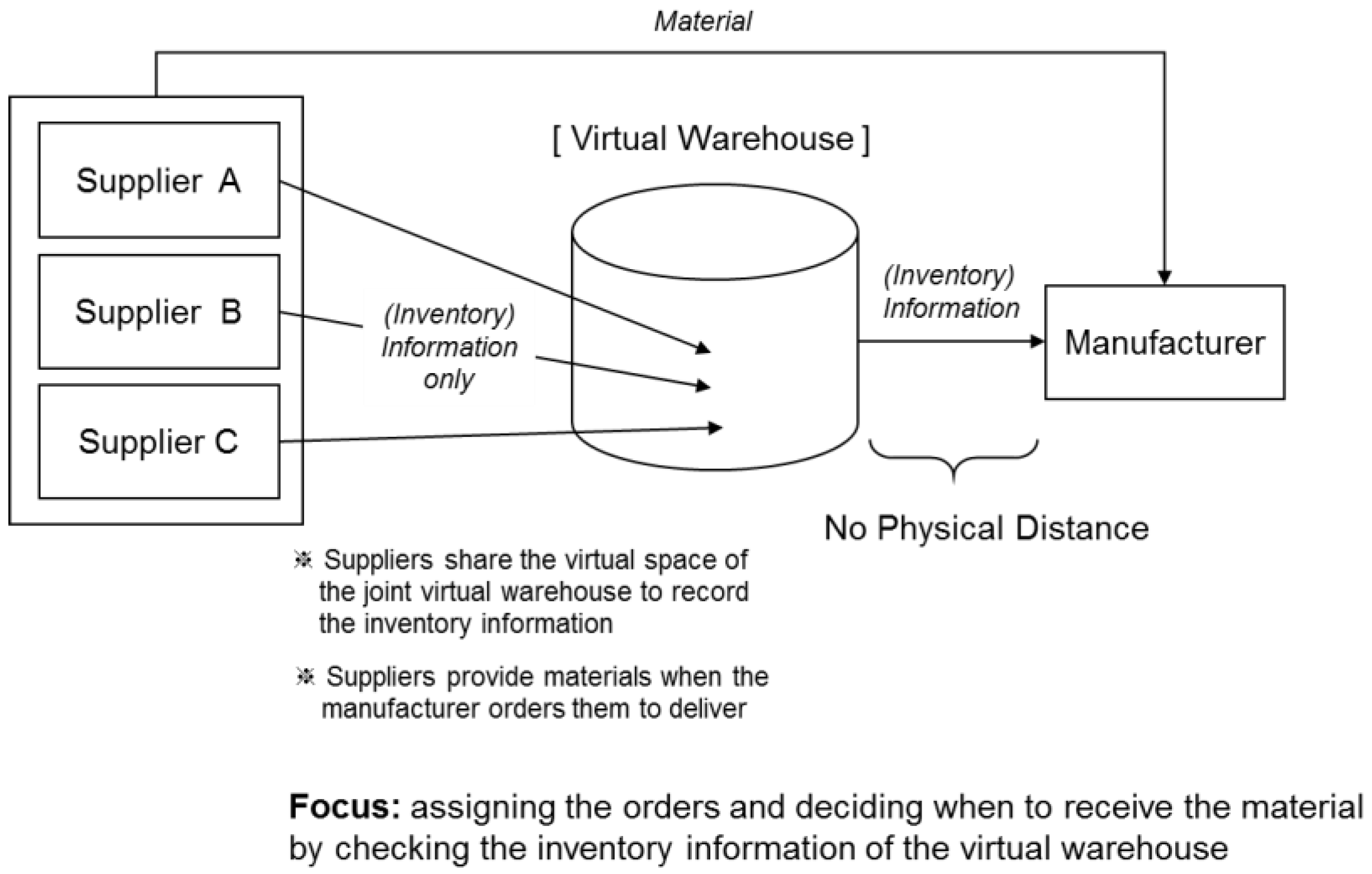
Figure 3.
The supply chain flow of Company H.

Figure 4.
The causal diagram of Company H.
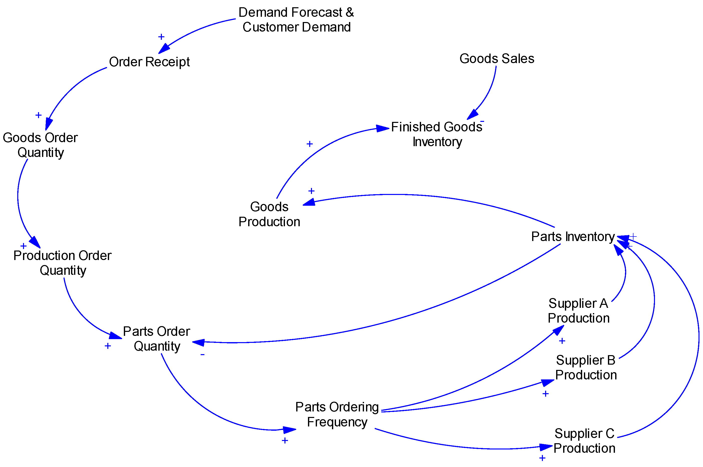
Figure 5.
Modelling without Virtual Warehouse.

Figure 6.
Modelling with Virtual Warehouse.
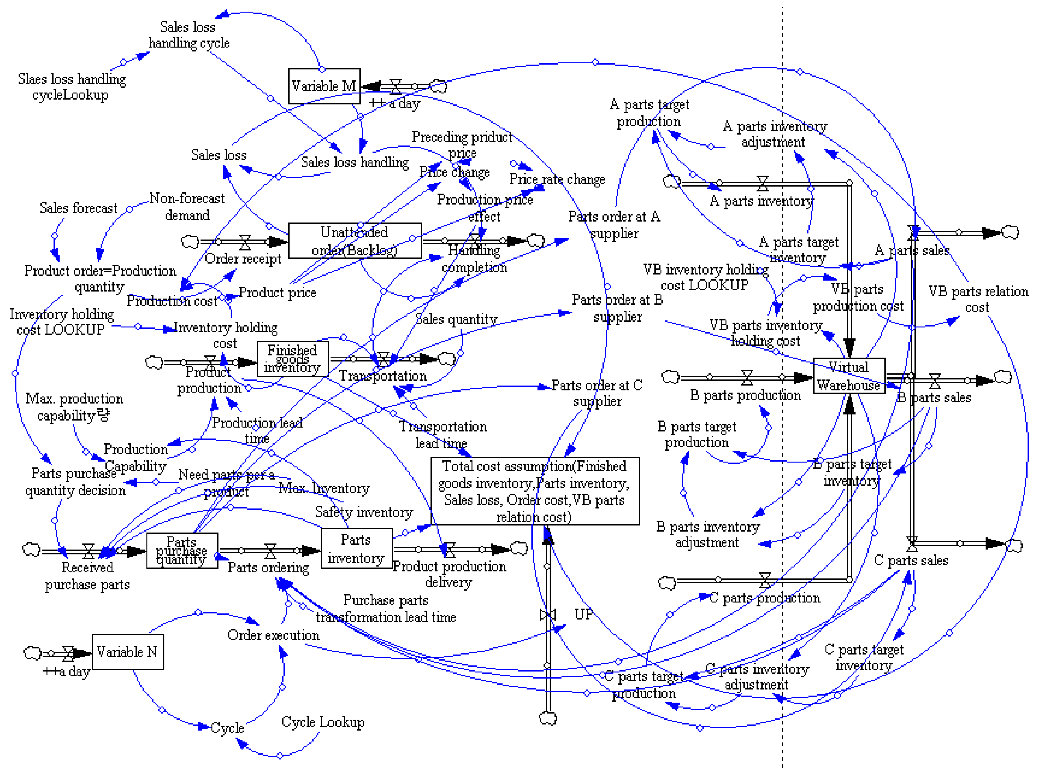
Figure 7.
Comparing the result of the simulation and real data.
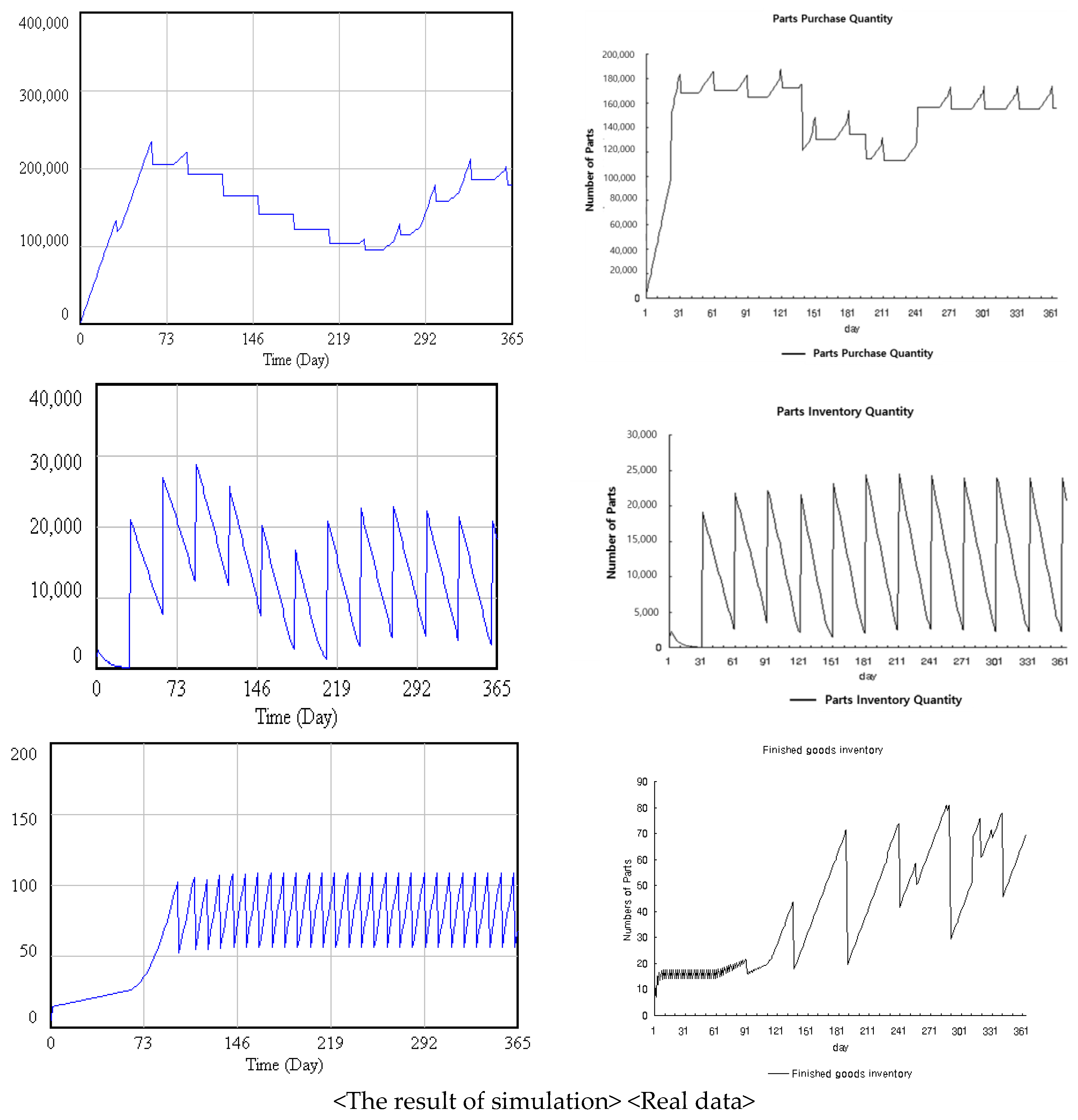
Figure 8.
Accumulated inventory quantity.

Figure 9.
Example of the joint pick-up and transport.
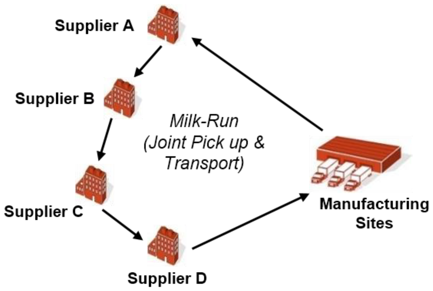
Figure 10.
Generalization of the proposed simulation model. (a) Generalized supply chain; and (b) generalized causal diagram.
Figure 10.
Generalization of the proposed simulation model. (a) Generalized supply chain; and (b) generalized causal diagram.

Table 1.
The brief comparison between Discrete Event Simulation and System Dynamics.
| Criteria | DES (Discrete Event Simulation) | SD (System Dynamics) |
|---|---|---|
| Representation | Network of queues and activities | System as set of stocks and flows |
| Change of states | Changes at discrete points of time (irregular discrete time steps) | Changes continuously over time (small discrete steps of equal length) |
| Setting of attributes | Specific attributes are assigned to each entity | Individual entities are not specifically modelled, but they are represented as a continuous quantity in a stock |
| Application areas | Appropriate when analyzing the problems at an operational or tactical level | Appropriate when taking a ‘distant’ perspective (i.e., strategic) where events and decisions are seen in the form of patterns of behavior and system structure |
Table 2.
Experimental results.
| Before | After | Discrepancy | GAP (%) | |
|---|---|---|---|---|
| Accumulated inventory quantity | 25,067 | 19,368 | 5699 | 22.7 |
| Accumulated part purchase quantity | 53,927,730 | 48,320,775 | 5,606,955 | 10.4 |
| Accumulated unattended order (backlog) | 80,567.49 | 75,006.29 | 5561 | 6.9 |
| Parts transportation cost | 8,868,000 | 7,944,000 | 2,336,500 | 26.3 |
| Accumulated total cost | 174,220,635 | 154,580,608 | 19,640,027 | 11.3 |
| The cost per a day | 477,317 | 423,509 | 53,808 |
Table 3.
The results according to the change of parts order cycle.
| Parts Order Cycle | The Yearly Total Order | Avg. Parts Purchase Quantity per Order | Accumulated Parts Inventory | Accumulated Finished Goods Inventory | Accumulated Assumptive Total Cost * | Avg. Sales Loss per Year |
|---|---|---|---|---|---|---|
| 30 days | 28,800 | 132,385 | 4,846,823 | 19,095 | 162,406,410 | 602 |
| 14 days | 62,400 | 65,598 | 3,679,455 | 19,433 | 153,372,873 | 553 |
| 7 days | 124,800 | 33,854 | 3,693,012 | 18,790 | 153,464,094 | 486 |
* The cost per order = 2400 Korean Won (2.4 USD).
© 2018 by the authors. Licensee MDPI, Basel, Switzerland. This article is an open access article distributed under the terms and conditions of the Creative Commons Attribution (CC BY) license (http://creativecommons.org/licenses/by/4.0/).
Share and Cite
MDPI and ACS Style
Jung, H.; Jeong, S. The Economic Effect of Virtual Warehouse-Based Inventory Information Sharing for Sustainable Supplier Management. Sustainability 2018, 10, 1547. https://doi.org/10.3390/su10051547
AMA Style
Jung H, Jeong S. The Economic Effect of Virtual Warehouse-Based Inventory Information Sharing for Sustainable Supplier Management. Sustainability. 2018; 10(5):1547. https://doi.org/10.3390/su10051547
Chicago/Turabian StyleJung, Hosang, and Sukjae Jeong. 2018. "The Economic Effect of Virtual Warehouse-Based Inventory Information Sharing for Sustainable Supplier Management" Sustainability 10, no. 5: 1547. https://doi.org/10.3390/su10051547
Note that from the first issue of 2016, this journal uses article numbers instead of page numbers. See further details here.