Article

Spatio-Temporal River Contamination Measurements with Electrochemical Probes and Mobile Sensor Networks

by
Iván P. Vizcaíno
1,*,
Enrique V. Carrera
1,
Sergio Muñoz-Romero
2,3,
Luis H. Cumbal
4 and
José Luis Rojo-Álvarez
2,3
1
Departamento de Eléctrica y Electrónica, Universidad de las Fuerzas Armadas ESPE, Av. General Rumiñahui s/n, 171-5-231B Sangolquí, Ecuador
2
Departamento de Teoría de la Señal y Comunicaciones y Sistemas Telemáticos y de Computación, Universidad Rey Juan Carlos, Camino del Molino s/n, 28943 Fuenlabrada, Spain
3
Center for Computational Simulation, Universidad Politécnica de Madrid; Boadilla, 28223 Madrid, Spain
4
Centro de Nanociencia y Nanotecnología, Universidad de las Fuerzas Armadas ESPE, Av. General Rumiñahui s/n, 171-5-231B Sangolquí, Ecuador
*
Author to whom correspondence should be addressed.
Sustainability 2018, 10(5), 1449; https://doi.org/10.3390/su10051449
Submission received: 28 March 2018 / Revised: 25 April 2018 / Accepted: 1 May 2018 / Published: 7 May 2018
(This article belongs to the Special Issue Information and Communications Technologies (ICT) for Sustainability)

Abstract

:
The pollution of the rivers running through the cities or near to them is a current world-wide problem and requires actions and new technologically available approaches to control and restore those waters. In this work, we hypothesized that last-generation mobile sensor networks can be combined with emergent electrochemical probes and with recently proposed spatio-temporal analysis of the measurement dynamics using machine learning tools. With this purpose, we designed a mobile system to measure five variables: two environmental and three water quality variables in rivers: dissolved oxygen with an electrochemical probe, water temperature, electrical conductivity, air temperature and percentage of relative humidity using solid-state sensors, in each monitoring station. Our main contribution is a first mobile-sensor system that allows mobile campaigns for acquiring measurements with increased temporal and spatial resolution, which in turn allows for better capturing the spatio-temporal behavior of water quality parameters than conventional campaign measurements. Up to 23 monitoring campaigns were carried out, and the resulting measurements allowed the generation of spatio-temporal maps of first and second order statistics for the dynamics of the variables measured in the San Pedro River (Ecuador), by using previously proposed suitable machine learning algorithms. Significantly lower mean absolute interpolation errors were obtained for the set of mean values of the measurements interpolated with Support Vector Regression and Mahalanobis kernel distance, specifically 0.8 for water temperature, 0.4 for dissolved oxygen, 3.0 for air temperature, 11.6 for the percentage relative humidity, and 33.4 for the electrical conductivity of the water. The proposed system paves the way towards a new generation of contamination measurement systems, taking profit of information and communication technologies in several fields.

1. Introduction

The continuous increase in population, urbanization, industrialization, and energy demand have generated global climatic changes that have affected the quality of water from natural sources, especially the rivers. Large emissions of CO 2 (carbon dioxide) to the atmosphere (currently the concentration is about 500 ppm) affect rainwater because it can form carbonic acid inside the raindrop and decrease the pH to 5.8–6.2. Once rain falls into the river’s water, its pH can reach values below neutral, thus impacting the aquatic life [1,2]. In recent decades, there has also been a decrease in the water level of streams, rivers, and lakes, while watersheds and surface water deposits have been contaminated. According to data from the World Health Organization, up to 844 million people lacked a basic service of drinking water supply in 2015, a figure that includes 159 million people who depend on the untreated surface waters of lakes, ponds, rivers, or streams. The consumption of contaminated water is related to the transmission of diseases such as cholera, diarrheas, dysentery, hepatitis A, typhoid fever, and poliomyelitis [3]. Therefore, health prevention and environmental care require an efficient intervention of the authorities to manage water resources in a responsible manner. In this setting, water quality monitoring becomes a permanent activity within water management actions, especially in modern times where there are new technologies available that could help to improve the water vigilance.
Water quality monitoring methods range from traditional techniques such as taking samples from natural sources and their subsequent laboratory analysis, to modern methods through in situ monitoring networks for small, medium, and large areas [4,5]. For example, wireless technologies and solid-state sensors were used in China to monitor the water quality of fish hatcheries, in order to optimally maintain several environmental parameters and to reduce the long-term mortality rate [6]. Drinking water and wastewater monitoring systems have also been designed in industrial plants in Europe, North America, and Japan [7,8]. Other monitoring systems were also designed to detect the bacterial concentration in drinking water by means of portable electronic sensors with disposable measurement cells [9].
Current water quality monitoring systems use the traditional method of sample collection and subsequent analysis in the laboratory, and an improved method that uses wireless communication techniques and solid-state sensors. However, there are still limitations regarding the versatility of the referred sensors, for instance: cost, restrictions of the maximum number of samples per sensor, and energy consumption. On the other hand, the cost per monitoring campaign is considerable, due to the difficulty of accessing to the stations. Therefore, the lack of samples in those inaccessible points can limit the knowledge of the spatio-temporal behavior of the pollution in rivers.
On-site water quality monitoring is also performed with electrochemical probes. Among the advantages of these devices, we can mention the following: (1) versatility, since they can interact with solid, liquid, or gaseous contaminants, and even for the electrolysis products; (2) energy efficiency, owing to the electrochemical processes require low temperatures and pressures compared with their non-electrochemical counterparts; (3) safety, due to the harmless nature of the involved chemicals; (4) selectivity, because the operator can control the applied potential to selectively attack specific links, thus avoiding the production of byproducts; and (5) docile to automation, since the electrical variables used are relatively cheap if the monitoring programs are properly designed [10].
For a continuous measurement of water quality, there are several systems [11] with components such as remote stations, sensors with one or more suitable parameters, measurement recorders and GSM/GPRS (Global System for Mobile communications, GPS; General Packet Radio Service, GPRS) communication systems, land and satellite radio links, and via Internet. These systems have been developed for hydrological and water quality applications, in general. Quality parameters such as conductivity, temperature, pH, dissolved oxygen, chlorine, turbidity, among others are monitored [12]. The sensor devices of these variables have been evolved from the traditional ones based on the laboratory setups, such as, potentiometric, conductometric, mass spectrometry, ion-sensitive electrodes and amperometric sensors. Second generation are in situ sensors with the ability to measure in real time water quality parameters at the site of interest, such as biosensors, fiber optic sensors, lab-on-chip-sensors, electromagnetic wave sensors, fluorescent detection, and infra-red (IR) sensors [13]. Currently, there are multi-parameter sensor systems that not only record the measurements, but also have the capacity to process and transmit the data locally or remotely.
The preceding framework and the contributions to the present work can be summarized as follows: in [14], our group started to scrutinize usefulness of state-of-the-art non-uniform interpolation methods to estimate the spatio-temporal dynamics of relevant variables for water quality analysis usually taken in rivers. We restricted ourselves to benchmark well-known conventional interpolation algorithms with a machine learning algorithm known as k-Nearest Neighbors (k-NN), and it was shown therein that the use of basic machine learning based algorithm provided us with the best estimation of spatio-temporal dynamics. These conclusions were obtained by working with measurement campaigns at Machángara River. After this [15], we proposed the use of several enhanced statistical interpolation methods, specifically, we included a priori available information of the quality parameter measurements through the use of Support Vector Regression (SVR) algorithms. Two specific kernels showed relevant advantage when they were used for SVR in this application, namely, the Mahalanobis spatial-temporal covariance matrix and the bivariate estimated autocorrelation function. Given that it was possible to analyze with appropriate algorithms the spatio-temporal dynamics of the water quality measurements from limited resolution measurements, our main contribution here is to create a physical system allowing for increasing the temporal and spatial resolution of these measurements, which can represent a strong support to the conventional campaigns and yield a more detailed description of the signals, in terms of temporal sampling distribution and spatial sampling distribution.
Although a variety of methods of estimating real-life cases concerning sustainability have been used [16,17,18], one would have to study their suitability for non-uniform interpolation problems because such methods could suffer from overfitting, underfitting or a high computational cost when adjusting their free parameters, as it could be the case of artificial neural networks. To avoid these shortcomings, in this work, we have used techniques that adjust very well problems of non-uniform interpolation, as has already been shown in previous works [19]. We refer to the reader to [20] for good summaries on interpolation and, more specifically, nonuniform interpolation. These methods are k nearest neighbor (k-NN), Mahalanobis Support Vector Regression (Ma-SVR), and Autocorrelation Support Vector Regression (Au-SVR). The assessment of these methods were made in terms of the Mean Absolute Error (MAE) by using the Leave One Out (LOO) cross-validation technique. Among the different methods to select the mathematical model, LOO is one of the best options for interpolation algorithms with moderate number of samples, both to obtain a good adjustment of free parameters that allows a solution that generalizes well all the data avoiding the over-fit, and to more accurately estimate the performance of the models [21,22].
In this paper, we propose a new approach of spatio-temporal analysis of environmental variables through electronic components and new and electrochemical devices with their technologies, together with more recent mobile sensors (transceivers) using automatic learning tools. This represents a compilation of the most convenient elements from current and different fields in Information and Communication Technologies (ICT), working together and adequately combined. For this purpose, we created an electronic mobile system that is designed to measure water quality and air parameters. In particular, we use solid state sensors to measure the ambient and water temperatures, a probe based on salinity to determine the electrical conductivity, a resistive-type probe to amount the percentage of relative air humidity, and mainly an electrochemical probe of galvanic type that uses a membrane and electrodes submerged into electrolyte to quantify the content of dissolved oxygen. The novelty of this work is the use of a mobile electronic prototype and low-cost probes to quantify some water characteristics without using chemical reagents that could impact on the environment. On-site measurements were performed online and did not require any transportation of water samples and other related processes of an analytical laboratory. With the measurements obtained at nine different places and at different times (November–December, 2017) in the path of the San Pedro River (Ecuador), the spatio-temporal dynamics of the first and second order statistics of the above referenced environmental variables were determined. For the statistical treatment, we adapted previously developed algorithms of machine learning interpolation [14,15]. Measurement maps were built even in difficult-access places and also at different times that were not routinely recorded in the monitoring campaigns.

2. Materials and Methods

The San Pedro River is one of the four main rivers that receive wastewater discharges from Quito. This river passes through the peripheral area of the city and collects approximately 5% of wastewater. San Pedro River is in the southeast of Quito city (capital of Ecuador) and flows through a hydrographic basin called Guayllabamba, which is located at 2500 m above sea level, as seen in Figure 1. Its temperature ranges from 10 C to 29 C, and it goes through towns such as Tambillo, Amaguaña, and Sangolquí (Los Chillos Valley). These towns are surrounded by extinct volcanoes that behave as natural barriers to the cold air currents, resulting in a pleasant climate with an average temperature of 15 C. This environmental condition has transformed this area into an ideal region for residential suburbs and industrial settlements (textile and food).
Previous studies have already been conducted on the pollution of Machángara River [14,15], which receives approximately 75% of Quito residual loads, but no research has been performed about the San Pedro River pollution. According to the population and housing census of 2001 [23], the population growth in Los Chillos Valley (micro basin of Guayllabamba) was 16.85% between 2010 to 2015, and it will be 15.13% between 2015 to 2020. This growth will strongly affect the water quality of San Pedro River because it receives the liquid-waste discharges from domestic and industry sources in this area. In addition, no previous study has been conducted on the degree of contamination of this river. These circumstances have motivated us to carry out a detailed study of the water contamination of the San Pedro river and to scrutinize the available data gathered in campaigns up to year 2017.
Since in the San Pedro River has not been performed recent water quality investigations, in the areas described in Figure 1, we conducted a water quality study through 23 monitoring campaigns between 15 November and 4 December 2017. For the study, they were allocated nine monitoring stations along 18 km of the river (see Table 1), these stations were localized in three differentiated zones (agricultural, industrial and residential). The average monitoring time was 12 min and the variables analyzed were: water temperature, dissolved oxygen, water electrical conductivity, air temperature and percentage of relative humidity. The measuring device was previously calibrated in a laboratory of environmental remediation using a Mettler Toledo SG9 (SevenGo pro optical dissolved oxygen) multiparameter as the reference equipment under the environmental conditions of the laboratory. Calibration adjustments were also carried out at each monitoring site, especially for the dissolved oxygen probe by the double-point method using: (a) a dissolved oxygen standard solution of 0 mg/L for the first point; and (b) ambient temperature compensation values, atmospheric pressure values, and oxygen dissolved in the air for the second point. The measurements were collected through a micro-controlled system and stored in a laptop. Then, the digital treatment of the information was carried out using automatic learning algorithms to determine the spatio-temporal trends of the five variables.

2.1. Electrochemical Probes and Mobile Sensors

A system to monitor environmental and water quality parameters becomes more efficient if it does not require chemical reagents for the measurements [9]. Therefore, the advantages of a monitoring system with electrochemical probes are notorious compared to other more traditional methods (sample collection and transportation to a laboratory, pretreatment processes and use of reagents) to obtain the final measurements [14]. In general, to monitor the environmental contamination requires portable sensors with rapid response, robust with sufficient sensitivity, and long service life. Among some aspects that should be taken into consideration when choosing electrochemical sensors are: selectivity, concentration range, calibration precision, measurement response time, and technological availability disposable, reusable, or renewable sensors [24].
The electrochemical devices that are used for environmental monitoring are: amperometric or voltammetric, potentiometric, and conductometric. The first group is based on the application of a potential through two electrodes in order to oxidate or reduce electroactive species. In this case, the resultant current is measured. This measurement method is used for the dissolved oxygen probes. For the potentiometric sensors, an electrode or membrane potential is measured when a local equilibrium is reached at the sensor interface. In this second case, the potential difference informs us about the composition of a sample. Typical examples of such as devices are in situ pH or pCO 2 meters. Finally, conductometric sensors are related to the measurement of conductivity at different established frequencies [25].
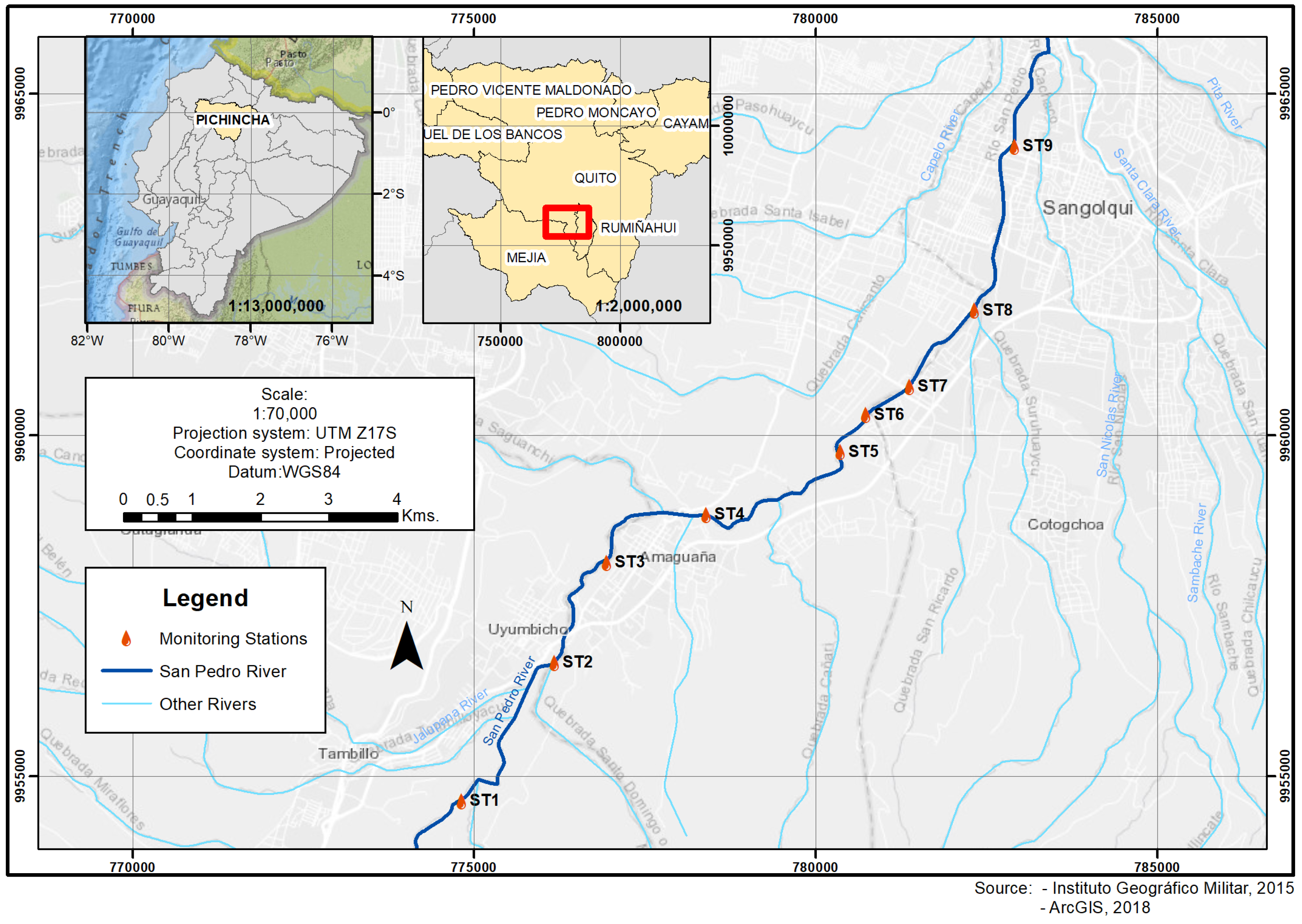
In the study area, we located three unique zones through which the San Pedro River flows: agricultural, industrial and residential (see Table 1). The factories were the first to reach the river banks a few decades ago and began to discharge their waste directly into the river. After the arrival of the factories to the San Pedro river basin, the population also began to grow, contributing with its waste to a greater contamination of the river. Both sources of wasterwater have common water quality characteristics such as dissolved oxygen (DO), electrical conductivity, and water temperature, dissolved oxygen being the the key parameter. If the DO concentration were in between 5 and 8 mg/L, water could be considered acceptable for most fish and other aquatic organisms while if the concentration were less than 5 mg/L, there would be a great risk of disappearance of organisms and sensitive species [26].
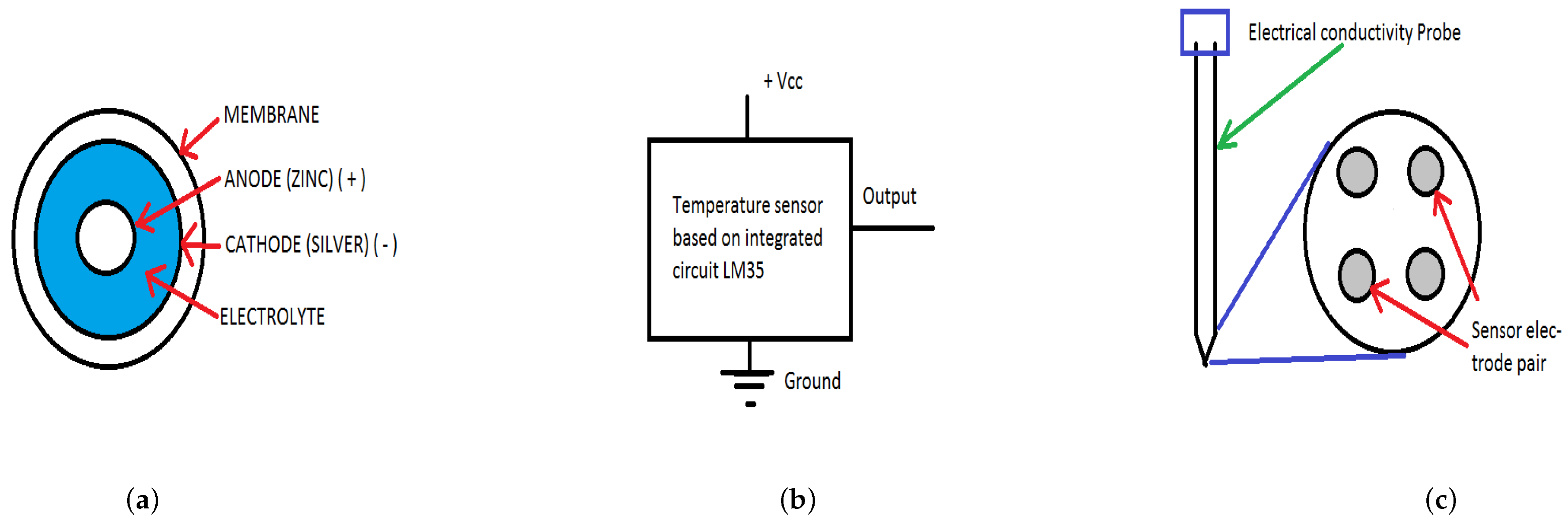
In this work, an electrochemical probe to measure the dissolved oxygen, an electrical conductivity probe for the estimation of total water salts, and an air temperature and percent of relative humidity sensor based on integrated circuits were used (see Figure 2). The dissolved oxygen probe includes a polyethylene membrane, a cathode, and an anode immersed in an electrolyte. The oxygen molecules that diffuse through the membrane at a constant rate [27] are reduced at the cathode and a voltage is produced. If there are no oxygen molecules, the probe will measure 0 mV. As the dissolved oxygen increases, the output measurement of the probe will also increase. The measurement of water temperature in the river was performed by using the integrated circuit device of the LM35 series. The LM35 device does not require any calibration or trimming to provide an accuracy around ± 0.25 C at room temperature and ± 0.75 C on the temperature range from 55 C to 150 C. Humidity measurements were obtained with a DHT11 integrated circuit device, which includes a resistive type humidity sensor, and a negative temperature coefficient for temperature measurement. This sensor was connected to a high performance 8-bit micro-controller, hence offering good quality measurements with a quick response, interference reduction, and low cost. Each DHT11 measuring device was carefully calibrated in the manufacturer laboratories to obtain accurate measurements of humidity. The calibration coefficients were stored in the OTP (One-Time-Programmable) memory, which was used by the sensor for each measurement [28]. The technical specifications of the probe and sensors can be seen in Table 2.
The monitoring campaigns were carried out following the order of geographical positions of the stations, starting from ST1 to ST9 (see Table 3). The sampling dates were chosen according to the climatic conditions that allowed access to the monitoring stations, and to the administrative permissions to access the sites by the landowners of factories or housing complexes. At each monitoring site, the following activities were performed: (1) calibration of the dissolved oxygen probes and the conductivity meter for the actual environmental conditions, considering particularly the ambient temperature, as this affects the second calibration point of the dissolved oxygen probe; (2) setting up the prototype, probes and sensors in a safe place, in such a way that the probes can be extended up to a distance of 1 m between the river border and the water; (3) starting the measurement program at least 10 s after having inserted the probes into the water, so that the transient measurements at the starting time periods can be released; (4) stopping the information recording program at least 10 s before removing the probes from the water; and (5) verification of the data collection, cleaning up probes and sensors with distilled water, and cleaning up with towel paper the solid part of the measurement system.

Mobile Sensor

Generally, in a water quality monitoring program, the monitoring objectives are established, indicating the variables that are to be investigated, the monitoring sites and when these measurements will be made. It is also necessary to know how the collection of samples will be carried out, what tools will be necessary for the analysis, and then the interpretation of the results [
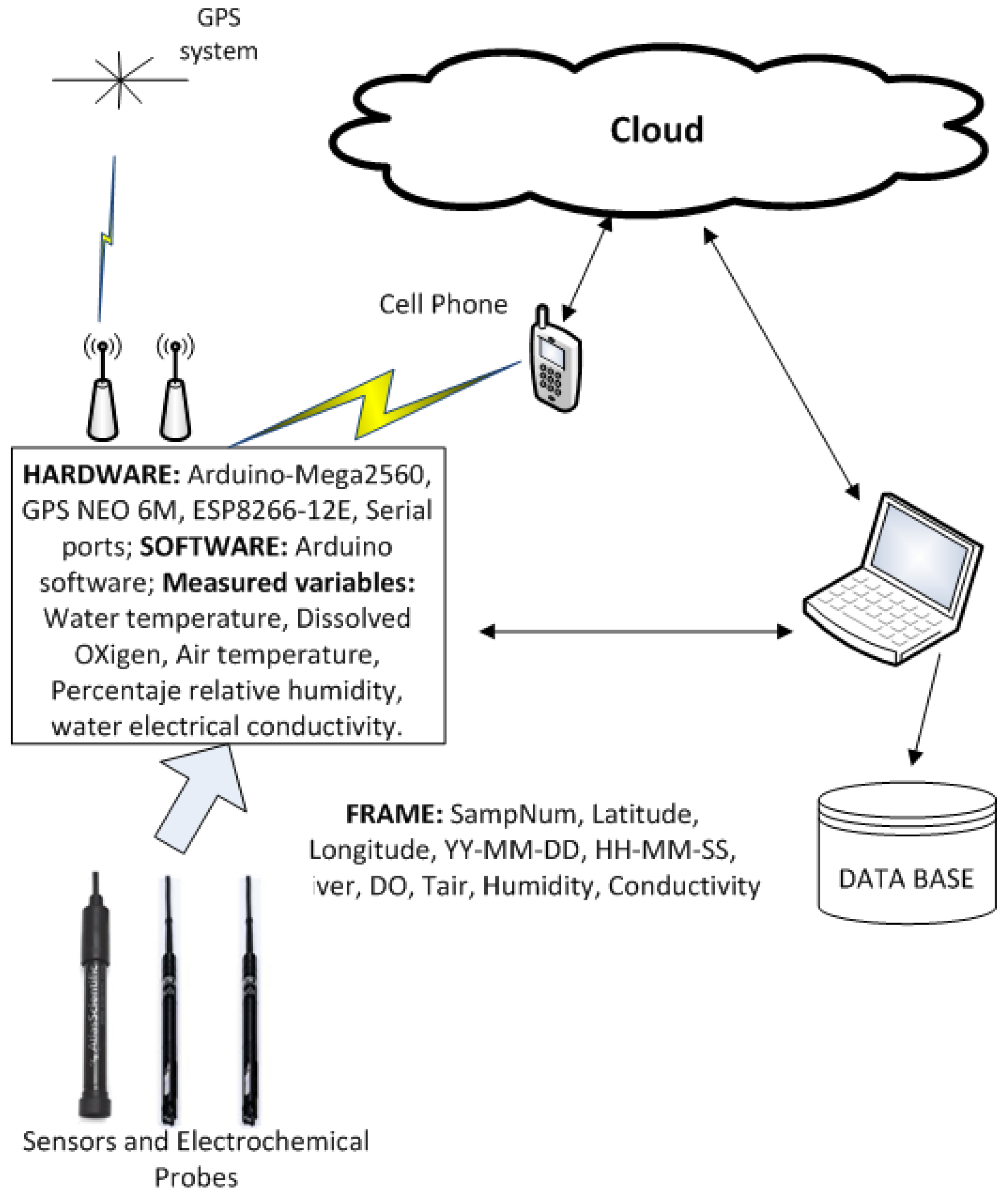
29]. The provision of a mobile prototype that allows online samples to be collected at any point in the study area and stored for later analysis is beneficial since it facilitates monitoring tasks. Although the monitoring sessions could be of short duration, the sum of all the sets of samples will allow forming databases with which studies of spatio-temporal trends of the variables of interest can be carried out. In the present work, micro-controlled devices were used, such as Arduino-Mega 2560 for the acquisition of data from the probes, GPS NEO 6M (Global Positioning System) for capture latitude, longitude, date and time during each monitoring session, and ESP8266-12E for the wireless transmission of information. This data set constitutes important information that could be stored for every campaign where it could be sent to the cloud for remote analysis or be stored in local form through a laptop and make a database of pollution water data. The portability of this prototype is due to some features as its battery durability, low weight, low cost, an easy software to manipulate, and simple calibration process.
In the market, there are multiparameter probes that allow for measuring water quality variables and datalogger to capture the information locally or remotely. These devices are very expensive for multiparameter measurements even without the availability of procedures for data analysis. In contrast, current-microcontrolled devices are cheap, easy to program, providing great versatility of applications to users and can also be adjusted to specific needs once they are coupled with medium-cost electrochemical probes. Thus, the great advantage of having electronic devices with their own software to perform the tasks of water quality monitoring is evident, which is moreover sensitive to the needs of researchers.

2.2. Electrochemical Probes and Mobile Networks

The prototype developed in this work is depicted in Figure 3. The measurements of the five variables are made at each monitoring site through a microcontroller electronic system (Arduino Mega 2560, GPS NEO 6M, ESP8266-12E, 12 V battery, control software created by ourselves to capture data and frame formation periodically) and the electrochemical probes. These five variables then adhere to the location information of the GPS, the date and the time duration of the measurements for each monitoring site. Therefore, the final data set (Frame) consists of the following variables:
  • Sample number,
  • Latitude,
  • Longitude,
  • Year, month, day, hour, minute, second,
  • Water temperature,
  • Dissolved oxygen,
  • Air temperature,
  • Percentage of relative humidity,
  • Water electrical conductivity.
The sampling period was approximately 35 s and the average sampling time at each site was 12 min. This sampling time per session was not constant due to the difficulties of the place access, the vegetation that impeded the reception of the GPS signals and the limitations of the dissolved oxygen sensor whose membrane was saturated after an exposure time greater than 12 min for the waters of the San Pedro River. The final data set can be sent wirelessly to a mobile phone and then to the cloud for backup storage. You can also send the information through the Arduino serial port to a laptop and thus form a local database.
We have developed a software (for Arduino) to capture data and shape the frame to transmit it through the serial port, either to send it to the cloud through the wireless system (ESP8266-12E) thus forming a remote monitoring network of water quality and environment variables, or to transmit it directly via serial cable to a laptop that is a few meters from the monitoring site. It should be noted that one of the advantages of this prototype is its portability that allows several measurements in a single day, taking care of the corresponding calibrations in each monitoring site.
Table 3 shows the summary of the monitoring campaigns carried out and the measured variables. It is important to point out that from 15 to 19 of November 2017, measurements of the river temperature ( T w ), concentration of dissolved oxygen in the river water (DO), ambient temperature ( T a ) and percentage of relative humidity were performed. The conductivity were not measured in this time period because the probe was not available yet. It is also relevant to remark that weather conditions in the study are unique. For example, in a single day, we could have a pleasant climate of 15 C without wind and rain, in the morning. In the afternoon, at about 2:00 p.m., the temperature could rise to 27 C with dry air, and approximately at 4:00 p.m. the temperature could drop to about 10 C and experiencing heavy rain. Therefore, it was necessary to carry out the measurements in that time span since the weather was more stable; however, on 15 and 22 of November 2017, it was raining. Additionally, from 22 November 2017 to 4 December 2017, measurements of five variables were carried out, including the water electrical conductivity. A field campaign description is provided in Figure 4.
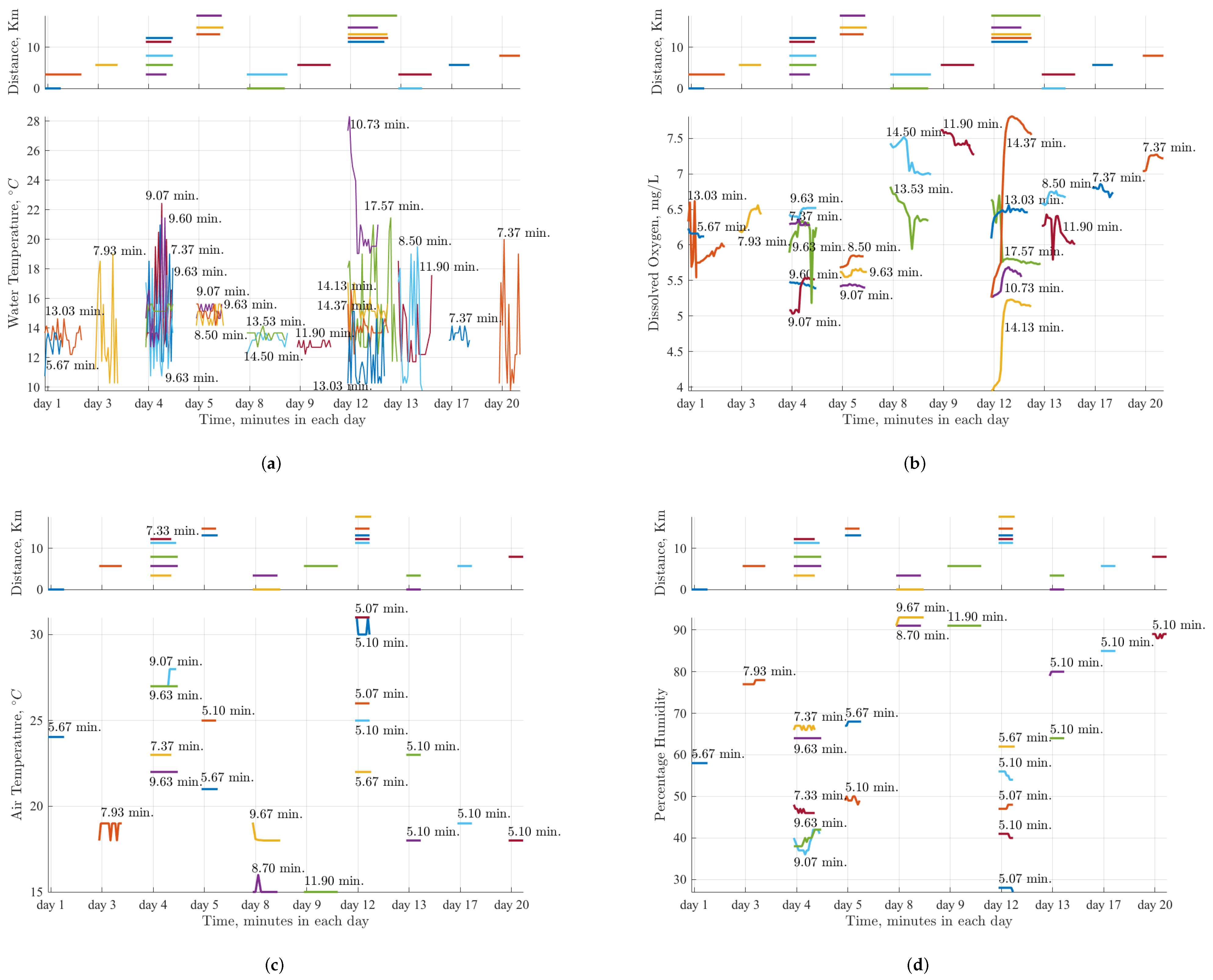
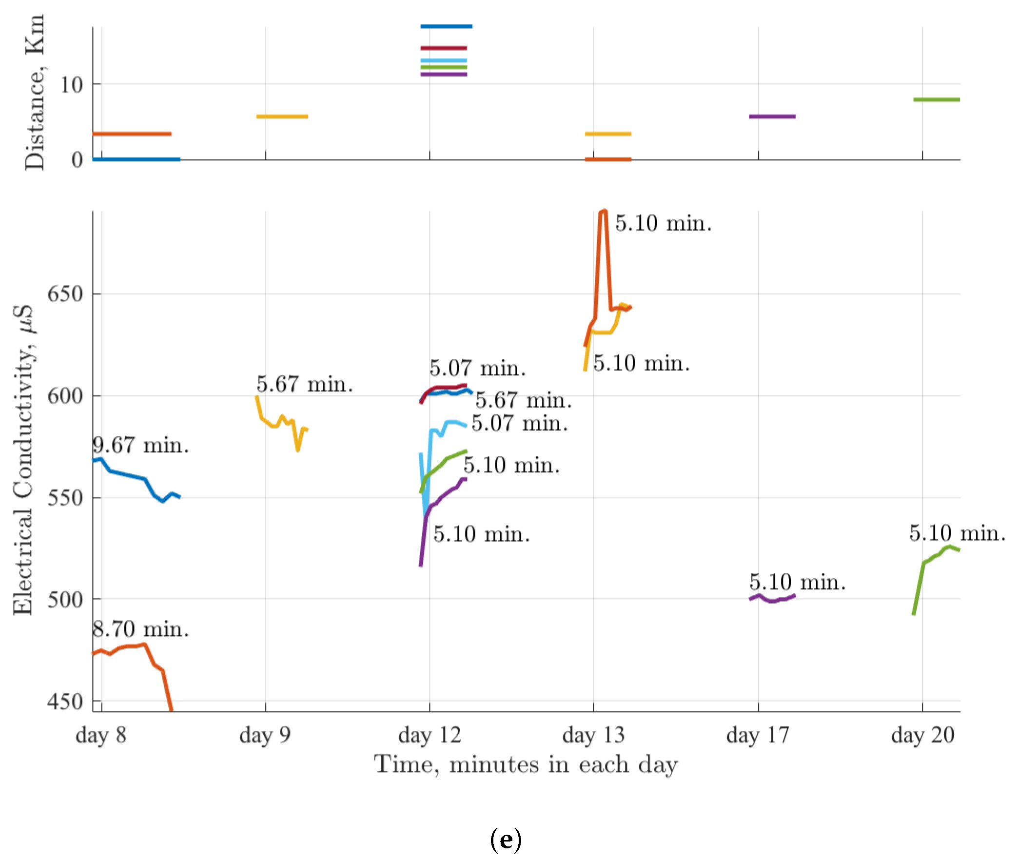
Because the field campaigns were carried out at separate monitoring stations with non-uniform distances and non-uniform times, the measurements of the five variables were different for each campaign and for the final sample sets. Figure 5 shows measurement values of the five variables in a time period of less than 100 sampling hours. Panel (a) represents the behavior of the river temperature, in which the measurement variability is noticeably larger than in the other variables. Panel (b) represents the trend of dissolved oxygen, likewise, its variability is lower than the river temperature, but still larger than the last three variables included in Figure 5. Panels (c)–(e) show the dynamics of air temperature, percentage of relative humidity, and electrical conductivity. It is seen that less spatial variability and highly regular behavior seems to be present. As expected, there could be a direct relationship between the measurement variability and the sensor quality for each. For example, the temperature in the water body of the river does not usually change abruptly. Thus, the variations observed in the measurements could be partially attributed to the quality of the semiconductor device used in this investigation.

2.3. Algorithms for Spatio-Temporal Dynamic Analysis

The proposed system allows us to measure an environmental variable in each location in a short time period and likely moving in space. In previous works [14,
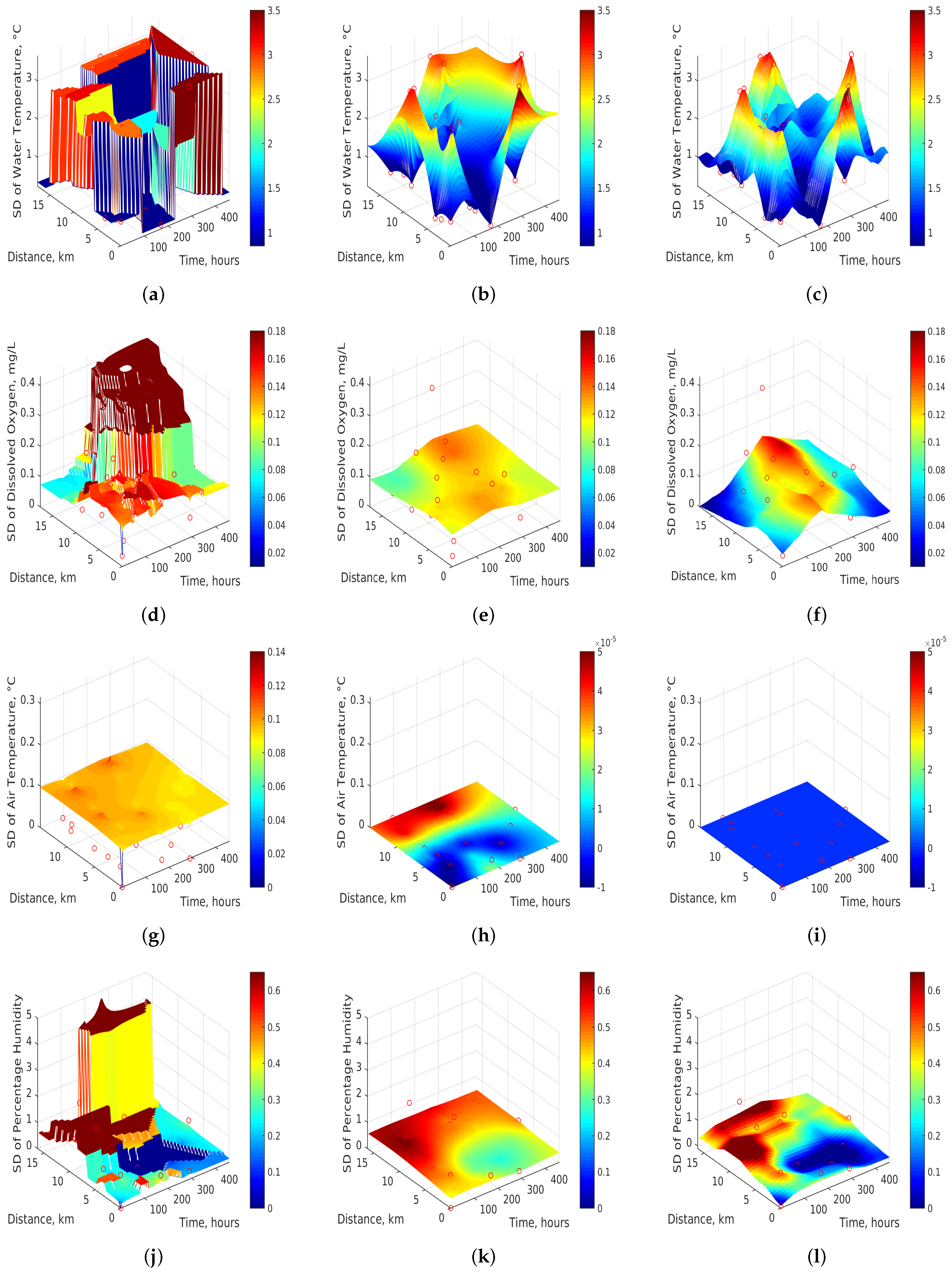
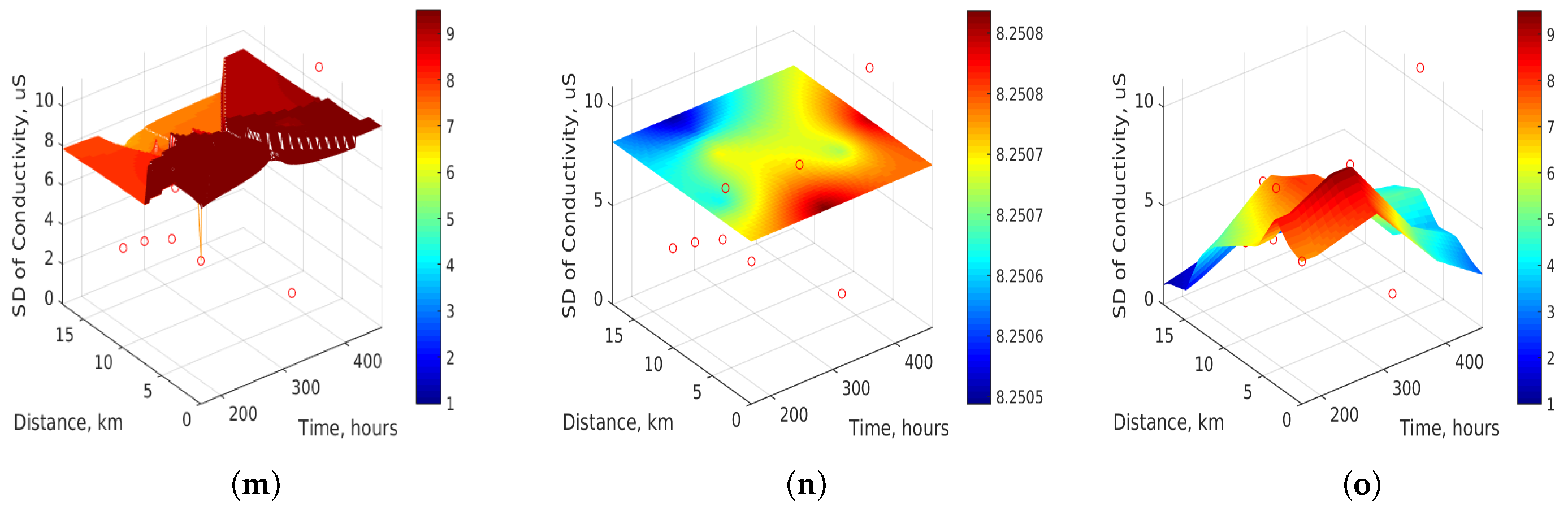
15], the dynamics of the variables resulting from the monitoring campaigns were represented using machine learning and advanced interpolation techniques. In this work, the availability of measurements sets for each location allowed us to calculate the mean and the standard deviation, hence yielding a map representation of the first and second order statistics of the spatio-temporal dynamics. This better exploits the information of the resulting data and gives a more complete description of the environmental variables.
According to purpose of the described system, we needed to analyze the data of our campaigns to monitor measurements on each variable sampled at different times and spatial locations. If we denote by ν a given environmental variable to be measured, its spatio-temporal distribution can be denoted as:
ν ( d , t ) ,
where d is the distance along the river path in a downward direction, usually starting from a zero reference point, and t is the time elapsed in a given area of consecutive sampling. We call this subset of consecutive samples at a geographically region with moderate displacements a session, and, in each session, we take a number of separate samples in time and space, that is:
s i = { ν ( d j , t j ) , j = 1 , , N i } ,
where N i is the number of samples acquired during that session. The set of measures of ν ( d , t ) in a session is obtained as:
{ s i } = j = 1 N i ν ( d , t ) δ ( d d j , t t j ) = j = 1 N i ν ( d j , t j ) δ ( d d j , t t j ) ,
where δ ( d , t ) is the Dirac’s delta function in our two-dimensional domain. A measurement campaign is the set of measurement sessions for the same variable and is denoted as:
V i = { s 1 , s 2 , s 3 , , s N i } ,
and the sessions are numbered by i = 1 , , N ν , where N ν is the total number of sessions for variable ν .
We can characterize each session by using a statistic p applied to that set of samples, for example, if M ( V i ) and S ( V i ), with i = 1 , , N ν , represent the sample average operator and the sample variance operator when applied to the samples of session V i , we have that M ^ ( d , t ) and S ^ ( d , t ) represent the estimated spatio-temporal dynamics for the first and second order statistics of that variable.
At this point, we need to introduce methods to provide us with this estimation from the available samples. Following previous works, we scrutinize here three of the algorithms that showed better performance in the analysis of Machángara River. First, the k Nearest Neighbors (k-NN) algorithm is a simple procedure that has been successfully used to interpolate multidimensional data with low computational burden. Second, the Support Vector Machine (SVM) algorithm has been previously used to estimate the spatio-temporal dynamics of contamination measurement in rivers, and it was shown that Mahalanobis and autocorrelation kernels often outperformed k-NN. Here, we scrutinize these three algorithms, which are next summarized [14,15]. We will denote by p j = ( d j , t j ) the spatio-temporal coordinate vector, and by f the measured variable or its estimated statistic, i.e., f is here a generalized notation for ν , M, and S, according to the analysis context.
One of the advantages of k-NN algorithm is that it is easy to implement it in software, providing robust estimates when a cross-validation technique is used [30]. The estimation of new values for targets p t is computed from the set of k closest neighbors. In addition, each selected neighbor p l , with l = 1 , , k , uses a weighted function according to its corresponding distance. The most common used distances are the Euclidean, Minkowski, Mahalanobis, and Cosine distances. The Mahalanobis distance between two points p 1 and p 2 is defined by
d i s t M ( p 1 , p 2 ) = ( p 1 p 2 ) T Σ p 1 ( p 1 p 2 ) ,
where Σ p is the covariance matrix of the available dataset. With relation to the Euclidean distance, the Mahalanobis distance has important properties; for instance, the Mahalanobis distance is invariant to scale changes and variable units, and it does not require any previous normalization. In addition, the matrix Σ p 1 accounts for the covariance among variables and possibly some redundancy effect. The estimation function f ^ ( p t ) is computed by the Distance Weighted Nearest Neighbor algorithm [31] as follows:
f ^ ( p t ) = l = 1 k w l f ( p l ) l = 1 k w l ,
where f ( p l ) represents the value of f at that neighbor sample, and w l are the weights defined in terms of the Mahalanobis distance as
w l = 1 d i s t M ( p t , p l ) 2 .
Consequently, the interpolation algorithm is polished by weighing the contribution of each neighbor according to their distance to target point p t . When p t matches exactly a p l neighbor, the denominator becomes zero; in that case, we just assign f ( p l ) to f ^ ( p t ) .
In this work, we additionally use kernel methods to interpolate and construct visualizations of the spatio-temporal dynamics of the measured water quality variables. Under this approach, kernel methods can be very useful when the statistical structure of the variables has been taken into account [32,33]. Probably the most well-known algorithm of the SVM is the classification one, but also good results have been obtained when addressing the solution of nonlinear regression applications.
Vapnik proposed to use the ϵ -insensitive loss function to obtain scattered solutions in the SVR algorithm [34,35]. Being ϵ > 0 , then we can define
( u ) = | u | ϵ = 0 , | u | < ϵ , | u | ϵ , otherwise .
This loss function sets to zero any error smaller than ϵ providing also robustness against outliers. The regression function construct a tube around the true function in order to estimate it, defining a margin around the function and treating the deviation as noise. In fact, the SVR model used in this study applies the following nonlinear regression model:
f ^ ( p ) = w , φ ( p ) + b ,
where φ ( p ) is a nonlinear transformation to a higher dimensional space, and b is a bias term. Then, considering a dataset D = { ( p 1 , f 1 ) , , ( p N , f N ) } , where N is the number of observed samples, the ν -SVR algorithm states that the function to minimize is [36]
1 2 w 2 + C ν ϵ + 1 N l = 1 N ( ξ l + ξ l * ) ,
where the first term is an L 2 regularization and the second one is the ϵ -insensitive loss function. Note that ϵ is the insensitivity parameter, C is a parameter that allows for tuning the compensation between the error tolerance and the softness of the regression. Additionally, ξ l and ξ l * are the slack variables representing error excesses for each sample ( p l , f l ) , and ν is the operative parameter that controls ϵ in terms of the maximum deviation from the measured value. Taking into account the following constraints:
ξ l , ξ l * 0 , l = 1 , , N ,
f l ( w , φ ( p ) + b ) ξ l + ϵ ,
( w , φ ( p ) + b ) f l ξ l * + ϵ ,
and, by using the Lagrangian functional, the solution to the nonlinear SVR is
w = l = 1 N η l φ ( p l ) ,
where η l , with l = 1 , 2 , 3 , , N are scalars, and samples p l for which η l 0 are the support vectors. Thus,
f ^ ( p ) = w , φ ( p ) + b = l = 1 N η l φ ( p l , φ ( p ) ) + b ,
which is equivalent to
f ^ ( p ) = l = 1 N η l K ( p l , p ) + b ,
where K ( · , · ) denotes a Mercer’s kernel, standing for the dot product independently from the nonlinear transformation or the dimensional space. In this work, ν -SVR is used to provide the estimation of the support vectors. Thus, the solution can be linearly expressed in terms of the kernel function and the available support samples.
Among the most usual Mercer’s kernels, we have the linear and Gaussian ones. In order to provide an improved performance, we have increased the statistical knowledge about the data structure within the algorithm through the following procedure. First, a conventional Gaussian radial basis function kernel (RBF-SVR) is used. In this case, the kernel is a bivariate function given by
K ( p i , p j ) = exp 1 2 σ 2 p i p j 2 ,
where the parameter σ allows for controlling the neighborhood of the samples influencing the solution. These structures can approximate the underlying function of a wide variety of data as long as σ is adequately tuned. Note that, in our study, we assume that changes in time and space dimensions follow similar dynamics because of radial symmetry. However, temporal and spatial variations will probably differ. Although normalization of inputs can alleviate this problem, other advanced kernels can be used without needing normalization.
Second, we propose to use a non-radially symmetric kernel, by using the covariance matrix of data (i.e., Σ x ). Then, an SVR with a Mahalanobis distance kernel (Ma-SVR) is created. This kernel equation is given by
K ( p i , p j ) = exp 1 2 p i T Σ p 1 p j ,
where the covariance-weighted distance between samples p i and p j is considered. Note that different spatial and temporal scales do not influence the basic distance.
Third, we use a SVR with an Autocorrelation kernel (Au-SVR), defined as
K ( p i , p j ) = R ^ ( p i p j ) ,
where R ^ ( q ) is the estimated two-dimensional autocorrelation function of the spatio-temporal dynamics. This kernel is a new type of SVR kernel that takes advantage of the autocorrelation value among samples. The autocorrelation is highly relevant function in digital signal processing, and a basic feature of stochastic processes. A main characteristic of the autocorrelation function is the symmetry with relation to the kernel matrix elements, K ( p i , p j ) = R ( p i p j ) = R ( p j p i ) . Note that the autocorrelation function is a robust measurement of the dependence among samples [37], depending only on the relative difference between elements rather than on their absolute values in the case of stationary processes.
This study looks for an optimum relationship between the amount of data, the quality of data approximation, and the parameters that characterize the approximation functions [38]. The problem is to find the best SVR structure that allows us to generalize the measurement samples in the presence of noise.

2.4. Motivation and Considerations for ICT on Sustainability

Several aspects can be considered for the use of ICT in the water monitoring environments, in terms of their technical and applied sustainability. On the one hand, the use of interpolation algorithms allows us to process the data to more efficiently extract the information. Specifically, the advantage of the interpolation algorithm in working with the closest neighbor criterion weighted by distance is that the measurements closest to the point to interpolate will be more important than those that are farther away. This is achieved by using the inverse of the square of the distance as the weighting criterion. This decreases the risk that all samples are taken into account for training and decrease the response time of the process. Another advantage is the increased robustness against data noise, especially against large data sets. As previously described, many estimation methods could be applied; however, the kernel methods are very popular and obtain very good benefits and generalization in non-uniform interpolation problems. Mercer kernels can be seen as bivariate functions and this type of kernel has the advantage of being able to do nonlinear learning in quadratic cost functions with a single minimum.
On the other hand, a ν -SVR is adopted in this study; however, other alternatives could be used, such as ϵ -SVR. Although performance of both algorithms would be similar when their free parameters are optimally selected, the free-parameter of ν -SVR is bounded above and below, ν ( 0 , 1 ) , and thus its adjustment is easier and optimal selection can be easier obtained. This is the reason why we have used ϵ -SVR. In addition, each dimension can present a different variation since non-radially symmetric kernels can assign different variation to each dimension, in this case these kernels have an advantage over symmetric kernels. One way of assigning that variation to each distance would be, for example, by applying the Mahalanobis distance with a Gaussian distribution to calculate the kernel, like the Mahalanobis nucleus we apply. Another option is to calculate the autocorrelation of the data in each dimension, as is done in the autocorrelation kernel.
From the acquisition of information perspective, there are two more water quality parameters that provide useful data when evaluating water of rivers, namely, COD and BOD5. However, there are few COD sensors for online measurements that can be hooked up to the designed mobile device. In regard to BOD5, it is usually measured in the laboratory after 5 days of sample collection, thus this parameter cannot be measured every 20 or 30 seg, during time periods of 12 min that lasted every measurement campaign. For the given reasons, we selected dissolved oxygen as the main river’s water quality parameter, which is directly related to both COD and BOD5 and can be measured at the same time as the other variables in situ.
San Pedro River was chosen because domestic discharges from Quito are collected through four rivers, Machángara, Monjas, San Pedro and Guayllabamba. The Machángara River receives approximately 75% of the total discharges of the city and passes through the urban area of Quito and studies of the spatio-temporal trends of some water quality variables have been carried out. However, the San Pedro River crosses a peripheral zone of Quito and receives approximately 5% of the total discharges of wastewater and is less polluted according to studies by EPMAPS (Metropolitan Public Company of Drinking Water and Sanitation) but requires urgent actions such as monitoring and control the water quality before it becomes contaminated as the Machángara River, although the San Pedro River encompasses three type of discharges: agriculture, industrial and residential wastewater, which may end up as an ugly mixture of liquid waste to be treated.

3. Results

3.1. Analysis of Spatio-Temporal Dynamics

As previously described, in this work, we use three interpolation algorithms for scrutinizing the dynamics of all variables. We want to stress that each algorithm could yield better performance than the others in different conditions, so it is highly recommendable to visualize the results for the three algorithms, in order not to trust only in a single one and also to be able to determine if the dynamics were well captured according to the consistency across the algorithms. Therefore, Figure 6 shows the results when using the actual measured values for all measurements, this is, for the 23 field sessions. Figure 7 shows the interpolation results when using the average values of each session. Finally, Figure 8 shows the results considering the standard deviation in each session for each variable.

3.1.1. Raw-Measurement Dynamics

Figure 6a–c show the dynamics of water temperature during all monitoring time and for the nine stations. The red circles show the original values, they appear closely one over another because the time duration of samples in the same session is only some minutes, while the time axis of the complete campaign is depicted in hours. We can observe that the results obtained with the k-NN algorithm are less smooth when compared to those obtained with Ma-SVR and Au-SVR. Figure 6d–f shows the spatio-temporal distribution of the raw measurements for dissolved oxygen. As in the previous case, it can be observed that the interpolation results with the k-NN algorithm are less smooth than those presented by the other two algorithms. In addition, it can be appreciated that, for the estimation results using Au-SVR, there is a noticeable difference in the edges with respect to those presented by k-NN and Ma-SVR, which can be due to loose estimation of the autocorrelation kernel. Figure 6 also shows the results of interpolation of air temperature, percentage of relative humidity, and electrical conductivity of water. As in the previous cases, the interpolation results with Ma-SVR and Au-SVR are better, based on the smoothing of the resulting signal, although Au-SVR continues to present a weak quality in the estimation at the edges.
From these representations, it can be observed that, for example, the river temperature raised to about 16.5 C in the last stations (ST7, ST8, and ST9, between 12 km to 17 km). These results would support the hypothesis that the temperature of the river water, in these stations, could have increased due to discharges of domestic and industrial wastewater from the nearby populated areas. In addition, in the places where the water temperature is high, the concentration of dissolved oxygen should decrease. In Figure 6e,f, it can be observed when the river temperature increases to 16.5 C, the oxygen drops to about 5.5 mg/L. On the contrary, when the temperature decreases to about 13 C, the dissolved oxygen concentration increases to approximately 7.5 mg/L. Panels (g), (h) and (i) show a rise in the ambient temperature to about 27 C at stations ST7, ST8, and ST9, at least in the last three-quarters of the total sampling time. Likewise, for these intervals of time and space, in panels (j), (k), and (l), it is observed that the percentage of relative humidity decreases to approximately 50% with the rise of the environmental temperature. The latter results show a coherence when relating the environmental temperature with the percentage relative humidity because they are inversely correlated. Panels (m), (n), (p) represent the dynamics from the row data for the water electrical conductivity in the spatio-temporal domain. The two last panels, (n) and (p), show two well-differentiated regions after 300 h (approximately 27 November 2017). The first region shows a rise in conductivity up to 630 μ S between stations ST1 to ST3 due to the presence of rain during these days (moderate concentrations of dissolved solids). It is also observed that said conductivity value decreases with the distance of travel, which can be attributed to the decantion of dissolved solids (sand and silt) into sediments of the river bottom. The second region shows a decrease in conductivity to about 480 μ S, which coincides with the decrease in rainfall in the studied zone, and, hence, the amount of dissolved solids in the river water.

3.1.2. Average-Measurement Dynamics

In view of the differences in the spatio-temporal dynamics of each of the environmental parameters analyzed from raw measurements, we believe it is informative to also estimate and represent the dynamics of the session-averaged values of these parameters, in order to verify more clearly the spatio-temporal trends. Figure 7 represents the interpolations of the five environmental parameters taking into account the average values for each monitoring session. Panels (a) and (b) represent the averaged values of the water temperature. It shows a spatio-temporal average value of 15 C, a minimum value of 13 C, and a maximum of 17 C. Panel (c) shows again somewhat different results at the boundaries, although the mean and maximum values are similar to the two previous ones. Panels (d), (e), and (f) show the averaged dissolved oxygen with similar trends between the maximum and the minimum values as those obtained for the raw measurements. Panels showing the session-averaged variations of the ambient temperature and the percentage of relative humidity display also the inversely proportional relation between these two variables. The panels that show the dynamics of the electrical conductivity of the water also show the different zones whose values oscillate between 480 to 620 μ S. Panels (a), (b), and (c) represent the interpolated values of the river water temperature based on the average values per each monitoring session. It should be noted that these estimates are more smoothed compared to the original values (Figure 6). It can be appreciated that the average temperature is 12 C, while the maximum is 16.5 C. The dynamics of dissolved oxygen is shown in Figure 7d–f, where two types of trends can be observed: First, a spatial trend from 12 km (ST6) to onwards. Over here, the concentration of dissolved oxygen in the water decreases due to the pollution with industrial and domestic wastewater. Next, a peak appears around 200 h (23 November 2017), with a value of 7.5 mg/L, which coincides with the rainy days recorded in the study area. This value tends to be kept at a lower constant value of 6.8 mg/L until the end of the monitoring days. The dynamics of the ambient temperature and the percentage of relative humidity are represented in Figure 7g–l. Similar to the results shown in Figure 6, an inverse relationship between the ambient temperature and the relative humidity can be observed in the average distribution of these variables. The electrical conductivity of water can be seen in Figure 7m–o. It clearly shows an increase in the concentration of dissolved solids in water with a maximum of 620 μ S between 200 and 310 h. As earlier explained, this trend is coincident with the rainy days in the study area.

3.1.3. Standard Deviation Dynamics

One of the most relevant aspects of this work is the analysis of the variability, in terms of the standard deviations, which is characteristic for each of the five environmental variables. In this setting, we can identify relevant information about the reliability of the used sensors, the methodology followed in the various measurement processes during the monitoring campaigns, the calibration requirements of the instruments, the stability times of the measurements before obtaining real and reliable measurements free of disturbances, or the method of data collection, among other aspects. Figure 8 presents these spatio-temporal dynamics of the standard deviations for each monitoring session. For instance, Panels (a), (b), and (c) represent the deviations for the measurements of the water temperature. The results based on the three algorithms show the greatest deviations among the other variables, that is, between 1 and 3.5 C with an average of 15 C as obtained in Figure 7. These results could mean that it is necessary to choose another kind of temperature sensor for the measurement of the temperature in the river water that is in constant circulation. Figure 8d–f represents the spatio-temporal dynamics of the standard deviations from dissolved oxygen. The three algorithms show that these deviations are between 0.02 and 0.18 mg/L, while the mean value obtained in Figure 7 was 6.2 mg/L. One of the reasons for a maximum of 0.18 mg/L can be seen in Figure 8, as the dissolved oxygen sensor used a polyethylene membrane that wears after several sessions of use and it needs to be replaced by another, or in its place a change of the whole sensor as happened in our case. Although the dissolved oxygen sensor was placed in favor of the water flow, wear was inevitable, which required us to change the probe in its entirety to ensure the calibration parameters according to the manufacturer instructions. Figure 8g–i represents the deviations of the air temperature in the monitoring zones. This is the case where the three algorithms show the lowest deviations, which could mean that the used sensor was the most appropriate. The average value of this variable, as shown in Figure 7, was 22.5 C, with a deviation from 1 × 10 5 to 5 × 10 5 , as shown in Figure 8. Deviations of percent relative humidity are shown in Figure 8, whose values are between 0 and 0.6%. The mean of this variable was 63.9% as seen in Figure 7. It should be noted that the sensing devices of the ambient temperature and the percentage relative humidity are manufactured in the same device, which is why the deviations are very small. Deviations in the electrical conductivity of the river water are shown in Figure 8m–o, where a minimum of 1 and a maximum of 9 μ S are observed, while the mean value of this variable was 567.7 μ S in Figure 7.

3.2. Behavior of the Interpolation Error

We have used three interpolation algorithms and one metric to know the accuracy degree of the interpolation. Although there are other metrics such as the RMSE (Root Mean Square Error), this parameter is, in turn, a function of three characteristics, such as the variability of the distribution of the error magnitude, the square root of the number of errors, and the magnitude of the average error MAE. Therefore, MAE is a natural measure of the average of errors and is not as ambiguous as RMSE [39]. Table 4 summarizes the mean absolute error (MAE) obtained by using the algorithms with the three data sets, namely, the raw measurements as a result of the 23 monitoring campaigns, the average values of the measurements, and the standard deviations obtained in each of the monitoring sessions for the five variables. In the set of errors obtained with the raw values of the measurements, the k-NN algorithm shows lower errors than the other two algorithms. This is primarily because the number of samples in the raw set (i.e., 431 for T w , 431 for D O , 261 for T a , 261 for H, and 122 for C) is much lower than the number of samples used in previous works [14,15]. In this case, the MAE is minimum for k equals 1 in most of the cases. In fact, we have noticed that Ma-SVR, and, in particular Au-SVR, require a considerable number of samples in order to reduce the MAE obtained through one-leave-out cross-validation.
On the other hand, the MAE obtained for the average values is normally greater than the MAE for the raw values. This result is due to the extremely low number of samples used in the set of average values (i.e., 24 for T w , 23 for D O , 19 for T a , 20 for H, and 12 for C). Because of this small number of samples, the MAE is minimum for k equals 1 in most of the cases, as mentioned before. The usage of k = 1 in the set of average values increases the error of the leave-one-out validation since nearest neighbors were clustered in a single sample. In the raw data set, k = 1 still produces small absolute errors due to the existence of similar neighbors. This last behavior was observed mainly in dissolved oxygen, percentage of relative humidity, and water electrical conductivity.
In addition, the MAE values of Ma-SVR are lower in three of the five variables than the MAE values of Au-SVR. Note also that, if we analyze the previous figures showing the interpolated spatio-temporal distributions, those results obtained with the Ma-SVR and Au-SVR algorithms are smoother and more likely to capture the dynamics than the k-NN algorithm spatio-temporal distributions, which seem to be highly influenced by bursts of outlier samples.

Comparison of the Dispersion of the Five Measures

Since the units of measurement of the temperature of the river water and of the ambient temperatures coincide, and knowing that the three other variables have different units of measurement, it is recommended to perform a comparative analysis of the dispersions found in the campaigns for each variable, in terms of standard deviation and mean values, as follows:
C v = ( σ v / X ¯ ) × 100 % ,
where C v is the variation coefficient, σ v is the standard deviation, and X ¯ is the average value of the measured variable.
Table 5 shows that the variable with the most dispersed measurements was the water temperature ( T w ), and the variable with the least dispersion in the measurements was the air temperature ( T a ). The measurements made with the prototype led to different values of dispersion quantified through the coefficient of variation. In practice, it is customary to consider that a coefficient of variation greater than 25% indicates a high degree of dispersion and therefore could have little representation in the arithmetic mean [40]. It can be observed that all values of variability coefficient had values less than 25%. Table 5 shows that the water temperature ( T w ) had the greatest dispersion (11.14%) with respect to the rest of the variables, while the variable that had the lowest dispersion (0.39%) was the air temperature ( T a ). These numerical results corroborate the graphical results shown in Figure 5 where the water temperature had the greatest dispersion. In this work, we have built a prototype for on-site measurement of three water quality variables in rivers: dissolved oxygen, electrical conductvity and temperature and two environmental: air temperature, percentage of relative humidity at the study area. For dissolved oxygen measurements, the maximum standard deviation was 0.17 mg/L, which represented 2.9%. For water temperature results, the standard deviation is higher compared to other evaluated variables (i.e., 1.6 that represents 11.41%) evaluated in the 23 monitoring campaigns. The water electrical conductivity sensor provides a maximum deviation of 9 μ S within an average of 567.7 μ S, and this is equivalent to 1.5%. Additionally, the percentage of relative humidity and ambient temperature sensors show deviations that do not exceed 0.01%.

4. Discussion and Conclusions

In relation to the space-temporal evaluation of the five variables analyzed, Figure 6 and Figure 7 show the results of the raw values and average values respectively during the sampling period between 15 November and 4 December 2017. The nine monitoring stations were located in three differentiated areas: agriculture, industry, and residential. The water temperature between stations ST1 to ST6 was maintained at about 14 C, while the temperature rose to about 16.5 C between stations ST7 and ST9. This is more likely because the river received water discharges from industrial and domestic sources. The concentration of dissolved oxygen decreases to 5.5 mg/L in the area where the temperature is higher (stations ST7 to ST9) while this value increased to 7.5 mg/L where the temperature remained around 14 C. This is in agreement with the change of oxygen solubility with temperature. In addition, when the ambient temperature rose around 27 C (between stations ST7 to ST9), it is observed that the percentage of relative humidity decreased up to 50%, while, when the ambient temperature decreased to approximately 16 C, the percentage of relative humidity rises to approximately 90%. It is known that, as air temperature increases, air can hold more water molecules, and its relative humidity decreases and, when temperature decreases, relative humidity increases. On the other hand, electrical conductivity remains around 630 σS in the first stations (ST1, ST2, and ST3) coinciding with rainfall in the area while approaching to the last stations, the electrical conductivity decreases to around 480 μ S. Surely this phenomenon is due to the gradual deposition of dissolved solids in the bottom of the river as the journey progresses. It seems that measurements of water quality and ambient parameters using the portable device are quite reliable and assures that the spatio-temporal interpolations are consistent.
In a previous work [41], features of a device are reported for measuring water quality with wireless data transmission, i.e., batteries of up to 6.8 Ah were used for a sensor node and a gateway. In our prototype, we use batteries with a lower current capacity (1.3 Ah), in which communication with the laptop (where the data is stored) is mostly via cable. Wireless communication, although available, is used less frequently. As a result, a battery endures approximately 10 h without recharging. Therefore, our prototype has less operational costs. The monitoring prototype developed in this work allows for monitoring three variables of water quality (water temperature, dissolved oxygen and electrical conductivity) and two variables of air quality (air temperature and relative humidity per percentage). The sampling period is approximately 35 s, and the maximum time of continuous measurements is 10 h, which gives the equipment the portability characteristic. This has a wireless communications module (802.11 b/g/n), low cost and reduced weight.

4.1. Kernel-Method Advantages

The spatio-temporal interpolation of each variable analyzed using each of the k-NN, Ma-SVR and Au-SVR algorithms was performed by adjusting its free parameters (see equations). For example, for the water temperature, an optimum k of 5 was obtained, which allowed the lowest MAE error of 1.34. The optimal parameters of Ma-SVR were ν = 0.86 and C = 0.19 with an MAE error of 1.33. For the algorithm Au-SVR, we obtained ν = 1 , C = 0.162 , γ = 0.001 and step = 0.297 (step is another tuning parameter) with an MAE of 1.28. The process time for the k-NN algorithm (few minutes) is the lowest compared to the rest of the algorithms that can be hours since the search method is used. The classic algorithm k-NN was used due to its great advantage over its low processing time; however, the interpolation surfaces are less pleasant than those presented by Ma-SVR and Au-SVR. This last algorithm has a longer processing time than the previous two, but, in Table 4, it is observed that, for the raw values and for the values of standard deviation, Au-SVR, at least in three of the five variables, has the lowest MAE error.
Regarding spatio-temporal dynamics, the use of interpolation of water quality measures through automatic learning has been proposed in [14,15]. The first and second order statistics allowed us to obtain graphical representations of the stochastic dynamics of the water pollution parameters of the river. In the same way, in this work, we have used these statistics and graphs that show the spatio-temporal dynamics of the five variables analyzed. For the set of average values, the lowest MAE errors were obtained using Ma-SVR for three variables, 1.34 (Water Temperature), 0.38 (Dissolved Oxygen), and 33.35 (Electrical Conductivity), while the slightly lower MAE errors for the other two variables were obtained with k-NN, 2.45 (Airt Temperature), and 11.25 (Percentage Humidity). Although k-NN was slightly better than Ma-SVR and Au-SVR algorithms, the best smoothness of these two algorithms compared with k-NN is notorious, which allows a better visualization of spatio-temporal trends.

4.2. Limitations of the Study

The limitations of the on-site measurements prototype fabricated in this work is the durability of the dissolved oxygen sensor because it uses a polyethylene membrane. The membrane gets saturated with colloids dissolved in water and with the time, thus the measurements are no longer stable. In our case, we had to replace the dissolved oxygen sensor after the 14th campaign, due to the fact that the measures marked values above 11 mg/L, and they were also unstable. Another limitation refers to the durability of the batteries. They lasted 10 h of continuous measurement before requiring a recharge. Another shortcoming is the loss of coverage of the GPS system in areas of medium and high vegetation. However, all these problems can be minimized if we use more stable water temperature sensors, electrochemical probes with longer membranes durability and higher gain antennas for the system GPS.
Nonetheless, it was noteworthy to demonstrate that this on-site measurement prototype has a great advantage compared to others due to its portability. It allows for short or long-term water quality measurements (less than 10 h) and several sites in the study area. Another advantage is that we are able to transfer the measurements in a wired or wireless way and these values can be recorded locally or in the cloud to create a historical record of the space-time dynamics.

4.3. Main Contributions and Future Works

This work proposes a microcontroller-based mobile system to measure water quality variables using electrochemical probes and solid-state sensors. This mobile-sensor system allows for carrying out water monitoring campaigns with increased temporal and spatial resolutions. The monitoring methodology for the mobile system has been evaluated through 23 monitoring campaigns in the San Pedro River, showing reliable and stable water quality values. In addition, machine learning algorithms have been applied for the interpolation of the monitored data, resulting in SVR with a Mahalanobis kernel showing the lower MAE due to the relatively small number of samples.
As future works, we have planned: (i) to perform longer monitoring campaigns to generate more representative spatio-temporal data for common water contaminants and different seasons; (ii) to increase the number of variables using other electrochemical probes for measuring variables such as pH, chlorine, or BOD5, among others; and (iii) to improve our microcontroller-based prototype in order to create a robust monitoring station that can travel along rivers sending information to the cloud. This last future work is without doubt a technological challenge that will revolutionize the way that water monitoring campaigns are performed currently.

Author Contributions

I.P.V., E.V.C., J.L.R.-Á., and L.H.C. conceived and designed the experiments. I.P.V. and S.M.-R. performed the experiments. E.V.C., L.H.C. and J.L.R.-Á. supervised the experiments. I.P.V. wrote the paper, and all authors contributed to reviewing all sections.

Funding

This work was supported in part by the Universidad de las Fuerzas Armadas ESPE under Research Grant 2015-PIC-004, and it has also been partially supported by Research Grants FINALE, and KERMES (TEC2016-75161-C2-1-R, and TEC2016-81900-REDT) from Spanish Government and PRICAM (S2013/ICE-2933) from Comunidad de Madrid, Spain.

Acknowledgments

The authors are grateful to Professor Marco Luna (IGN) for developing the cartography used in this work.

Conflicts of Interest

The authors declare no conflicts of interest.

References

  1. John, H.S.; Spyros, N.P. Atmospheric Chemistry and Physics: From Air Pollution to Climate Change, 2nd ed.; Wiley-Interscience: Hoboken, NJ, USA, 2006; pp. 959–960. [Google Scholar]
  2. Le Quéré, C.; Andrew, R.M.; Friedlingstein, P.; Sitch, S.; Pongratz, J.; Manning, A.C.; Korsbakken, J.I.; Peters, G.P.; Canadell, J.G.; Jackson, R.B.; et al. Global Carbon Budget 2017. Earth Syst. Sci. Data 2018, 10, 405–448. [Google Scholar] [CrossRef]
  3. World Health Organization. Drinking-Water. Available online: http://www.who.int/mediacentre/factsheets/fs391/en/ (accessed on 2 November 2017).
  4. Zhuiykov, S. Solid-state sensors monitoring parameters of water quality for the next generation of wireless sensor networks. Sens. Actuators B 2012, 161, 1–20. [Google Scholar] [CrossRef]
  5. Duan, W.; He, B.; Nover, D.; Yang, G.; Chen, W.; Meng, H.; Zou, S.; Liu, C. Water Quality Assessment and Pollution Source Identification of the Eastern Poyang Lake Basin Using Multivariate Statistical Methods. Sustainability 2016, 8, 133. [Google Scholar] [CrossRef]
  6. Xiuna, Z.; Daoliang, L.; Dongxian, H.; Jianqin, W.; Daokun, M.; Feifei, L. A remote wireless system for water quality online monitoring in intensive fish culture. Comput. Electron. Agric. 2010, 71S, S3–S9. [Google Scholar]
  7. Tseng, C.-L.; Jiang, J.-A.; Lee, R.-G.; Lu, F.-M.; Ouyang, C.-S.; Chen, Y.-S.; Chang, C.-H. Feasibility study on application of GSM–SMS technology to field data acquisition. Comput. Electron. Agric. 2006, 53, 45–59. [Google Scholar] [CrossRef]
  8. Vellidis, G.; Tucker, M.; Perry, C.; Kvien, C.; Bednarz, C. A real-time wireless smart sensor array for scheduling irrigation. Comput. Electron. Agric. 2008, 61, 44–50. [Google Scholar] [CrossRef]
  9. Grossi, M.; Lazzarini, R.; Lanzoni, M.; Matteuzzi, D.; Ricco, B. A Portable Sensor With Disposable Electrodes for Water Bacterial Quality Assessment. IEEE Sens. J. 2013, 13, 1775–1782. [Google Scholar] [CrossRef]
  10. Krishnan, R.; Ibanez, J. Environmental Electrochemistry; Fundamentals and Applications in Pollution Sensors and Abatement; Technology Books; Elsevier Science: New York, NY, USA, 1997; pp. 365–366. [Google Scholar]
  11. Agua y Medio Ambiente. Available online: http://www.panatec-agua.com/calidad-agua.php (accessed on 2 January 2018).
  12. LG SONIC. Available online: https://www.lgsonic.com/es/software-de-monitoreo-de-la-calidad-del-agua-en-tiempo-real/ (accessed on 10 January 2018).
  13. Adu-Manu, K.S.; Tapparello, C.; Heinzelman, W.; Katsriku, F.A.; Abdulai, J.-D. Water Quality Monitoring Using Wireless Sensor Networks: Current Trends and Future Research Directions. ACM Trans. Sens. Netw. 2016, 13, 1–37. [Google Scholar] [CrossRef]
  14. Vizcaíno, I.P.; Carrera, E.V.; Sanromán-Junquera, M.; Muñoz-Romero, S.; Rojo-Alvarez, J.L.; Cumbal, L.H. Spatio-Temporal Analysis of Water Quality Parameters in Machángara River with Nonuniform Interpolation Methods. Water 2016, 8, 507. [Google Scholar] [CrossRef]
  15. Vizcaíno, I.P.; Carrera, E.V.; Muñoz-Romero, S.; Cumbal, L.H.; Rojo-Alvarez, J.L. Water Quality Sensing and Spatio-Temporal Monitoring Structure with Autocorrelation Kernel Methods. Sensors 2017, 17, 2357. [Google Scholar] [CrossRef] [PubMed]
  16. Chen, X.Y.; Chau, K.W. A Hybrid Double Feedforward Neural Network for Suspended Sediment Load Estimation. Water Resour. Manag. 2016, 30, 2179–2194. [Google Scholar] [CrossRef]
  17. Olyaie, E.; Banejad, H.; Chau, K.W.; Melesse, A.M. A comparison of various artificial intelligence approaches performance for estimating suspended sediment load of river systems: A case study in United States. Environ. Monit. Assess. 2015, 187, 189. [Google Scholar] [CrossRef] [PubMed]
  18. Wang, W.; Xu, D.; Chau, K.; Lei, G. Assessment of River Water Quality Based on Theory of Variable Fuzzy Sets and Fuzzy Binary Comparison Method. Water Resour. Manag. 2014, 28, 4183–4200. [Google Scholar] [CrossRef]
  19. Sanroman-Junquera, M.; Mora-Jimenez, I.; Almendral, J.; Everss, E.; Caamaño-Fernandez, A.; Atienza, F.; Castilla, L.; Rojo-Alvarez, J.L. Automatic Location of Ventricular Arrhythmia using Implantable Defibrillator Stored Electrograms. Comput. Cardiol. 2010, 37, 749–752. [Google Scholar]
  20. José, L.R.-Á.; Manel, M.-R.; Jordi, M.-M.; Gustau, C.-V. Digital Signal Processing with Kernel Methods; Wiley: Hoboken, NJ, USA, 2018. [Google Scholar]
  21. Arlot, S.; Celisse, A. A survey of cross-validation procedures for model selection. Statist. Surv. 2010, 4, 40–79. [Google Scholar] [CrossRef]
  22. Ludmila, I.K. Combining Pattern Classifiers, Methods and Algorithms; Wiley: Hoboken, NJ, USA, 2004. [Google Scholar]
  23. Municipio del Distrito Metropolitano de Quito. La Planificación del Desarrollo Territorial en el Distrito Metropolitano de Quito; Technical Report; Municipio del Distrito Metropolitano de Quito: Quito, Ecuador, 2009. [Google Scholar]
  24. Brett, C.M.A. Electrochemical sensors for environmental monitoring. Strategy and examples. Pure Appl. Chem. 2001, 12, 1969–1977. [Google Scholar] [CrossRef]
  25. Grady, H.; Deepa, G.; Wang, J. Electrochemical sensors for environmental monitoring: Design, development and applications. R. Soc. Chem. J. 2004, 6, 657–664. [Google Scholar]
  26. Bain, M.B.; Stevenson, N.J. Aquatic Habitat Assessment: Common Methods; American Fisheries Society: New York, NY, USA, 1999. [Google Scholar]
  27. Jordan Press. Atlas Scientific Environmental Robotics V3.8 Dissolved Oxygen EZO; Technical Report; Jordan Press: New York, NY, USA, 2017. [Google Scholar]
  28. D-Robotics UK. DHT11 Humidity & Temperature Sensor. Available online: http://www.droboticsonline.com (accessed on 20 December 2017).
  29. Canadian Council of Ministers of the Environmental. Guidance Manual for Optimizing Water Quality Monitoring Program Design; Technical Report; Canadian Council of Ministers of the Environmental: Winnipeg, MB, Canada, 2015.
  30. Karl, S.; Truong, Q. An Adaptable k-Nearest Neighbors Algorithm for MMSE Image Interpolation. IEEE Trans. Image Process. 2009, 18, 1976–1987. [Google Scholar]
  31. Shepard, D. A two-dimensional interpolation function for irregularly-spaced data. In Proceedings of the 23rd ACM National Conference, Las Vegas, NV, USA, 27–29 August 1968; pp. 517–524. [Google Scholar]
  32. Soguero-Ruiz, C.; Guerrero-Curieses, A.; Palancar, F.J.; Bermejo, J.; Antoranz, J.C.; Rojo-Álvarez, J.L. Autocorrelation Kernel Support Vector Machines for Doppler Ultrasound M-Mode Images Denoising. In Proceedings of the Computing in Cardiology Conference, Vancouver, BC, Canada, 11–14 September 2016. [Google Scholar]
  33. Castro-García, B.; Sanromán-Junquera, M.; Guerrero-Curieses, A.; Trenor, B.; García-Alberola, A.; Rojo-Álvarez, J.L. Non-uniform Interpolation of Cardiac Navigation Maps Using Support Vector Machines with Autocorrelation Kernel. In Proceedings of the Computing in Cardiology Conference, Vancouver, BC, Canada, 11–14 September 2016. [Google Scholar]
  34. Clarke, B.; Fokoué, E.; Zhang, H.H. Principles and Theory for Data Mining and Machine Learning; Springer: New York, NY, USA, 2009; pp. 304–310. [Google Scholar]
  35. Hsieh, W.W. Machine Learning Methods in the Environmental Sciences; Cambridge University Press: Cambridge, UK, 2009; pp. 196–198. [Google Scholar]
  36. Chang, C.C.; Lin, C.J. Training ν-Support Vector Regression: Theory and Algorithms. Neural Comput. 2002, 14, 1959–1977. [Google Scholar] [CrossRef] [PubMed]
  37. Kong, R.; Zhang, B. Autocorrelation Kernel Functions for Support Vector Machines. In Proceedings of the Third International Conference on Natural Computation, Haikou, China, 24–27 August 2007. [Google Scholar]
  38. Vladimir, N.; Vapnik, V. Adaptive and Learning Systems for Signal Processing, Communications, and Control. In Statistical Learning Theory; Wiley: New York, NY, USA, 1998. [Google Scholar]
  39. Willmott, C.J.; Matsuura, K. Advantages of the mean absolute error (MAE) over the root mean square error (RMSE) in assessing average model performance. Clim. Res. 2005, 30, 79–82. [Google Scholar] [CrossRef]
  40. Murray, S. Estadística; McGrawHill: Madrid, España, 1991. [Google Scholar]
  41. Jieping, Y.; Huili, Y.; Weixing, W.; Guohui, J. Design of Real Time Monitoring System for Rural Drinking Water Based on Wireless Sensor Netwok. In Proceedings of the IEEE International Conference on Computer Network, Electronic and Automation, Xi’an, China, 23–25 September 2017. [Google Scholar]
Figure 1. Location of monitoring stations at San Pedro River. Based on data from IGM (Instituto Geográfico Militar), 2015.
Sustainability 10 01449 g001
Figure 2. Probes and sensors used in the measurement system: (a) galvanic probe, membrane and measurement kit for dissolved oxygen; (b) water river temperature sensor; (c) conductivity probe.
Sustainability 10 01449 g002
Figure 3. Electronic components of the prototype used in the measurements of environmental variables and water quality of the river. Data can be sent wirelessly to the cloud for storage and further processing, or the data can also be obtained directly through the serial ports.
Sustainability 10 01449 g003
Figure 4. Field campaign description of the measurement sessions: (a) satellite view of the monitoring stations that are located in agricultural, industrial, and populated areas; (bd) three types of stations can be distinguished, namely, slightly polluted, polluted by organic waste, and contaminated by textile waste; (eg) staff is calibrating the equipment, initiating the data record, and sensing the contamination variables in the river.
Sustainability 10 01449 g004
Figure 5. Spatio-temporal representation of the measurements for the five analyzed variables. Each time slot corresponds to a monitoring session (campaign) with a maximum duration of 12 min: (a) water river temperature; (b) dissolved oxygen; (c) air temperature; (d) percentage humidity; (e) electrical conductivity.
Sustainability 10 01449 g005aSustainability 10 01449 g005b
Figure 6. Spatio-temporal dynamics of the raw measurements from the environmental variables, by using k-NN (left column), Ma-SVR (center column), and Au-SVR (right column) algorithms: (ac) water river temperature; (df) dissolved oxygen in the river; (gi) air temperature at monitoring station; (jl) air percentage humidity; (mo) electrical water conductivity.
Sustainability 10 01449 g006
Figure 7. Spatio-temporal dynamics of the session-averaged measurements from the environmental variables, by using k-NN (left column), Ma-SVR (center column), and Au-SVR (right column) algorithms: (ac) water river temperature; (df) dissolved oxygen in river; (gi) air temperature at monitoring station; (jl) air percentage humidity; and (mo) water electrical conductivity.
Sustainability 10 01449 g007aSustainability 10 01449 g007b
Figure 8. Spatio-temporal dynamics of the SD Values in 2D of five variables by using the algorithms k-NN, Ma-SVR, and Au-SVR respectively in each column: (ac) water river temperature; (df) dissolved oxygen in river; (gi) air temperature at monitoring station; (jl) air percentage humidity; and (mo) water electrical conductivity.
Sustainability 10 01449 g008aSustainability 10 01449 g008b
Table 1. Monitoring stations used in San Pedro River. Parameter d corresponds to the distance from each station to the first one.
Station NumberStation Named (km)
ST1Populated area (Tambillo town)0.00
ST2Food factory3.39
ST3Textile factory5.70
ST4Sport fishing area7.94
ST5Agricultural area11.32
ST6South industrial zone12.26
ST7Center industrial zone13.15
ST8North industrial zone14.80
ST9Populated area of residential complexes17.69
Table 2. Technical specifications of the sensors used in water and air quality measurements.
SensorSpecifications
Dissolved oxygenAtlas Scientific Dissolved Oxygen Sensor, Range 0.01 to 35.99 mg/L, Accuracy +/− 0.05 mg/L, Data protocol UART (Universal Asynchronous Receiver-Transmitter) and I2C (Inter-IC bus), Calibration 1 or 2 points
Water temperaturePrecision centigrade temperature sensor, LM35 (Linear Monolithic), rated for full −55 C to water temperature 150 C, Linear + 10-mV/ C Scale Factor, 0.5 C ensured, accuracy (at 25 C)
Electrical conductivityElectrical Conductivity Tester 11+ Spectrum, Range 0 to 2000 μ S
Air temperature and humidityDHT11 (Digital Temperature & Humidity sensor) basic temperature - humidity sensor, Range 0 to 50 C temperature humidity readings +/− 2 C accuracy
Table 3. Dates of monitoring sessions conducted by each station and monitored variables. T w is the river water temperature, D O is the dissolved oxygen, T a is the air temperature at the station, H is the percentage relative humidity existing in the river bank, and C is the electrical conductivity of the river water. The total monitoring time was about 459 h through 20 days.
StationDates and Measured Variables
15 Nov.17 Nov.18 Nov.19 Nov.22 Nov.23 Nov.26 Nov.27 Nov.1 Dec.4 Dec.
ST1 T w , D O , T a , T w , D O , T a , T w , D O , T a ,
H H, C H, C
ST2 T w , D O , T a , T w , D O , T a , T w , D O , T a , T w , D O , T a ,
H H H, C H, C
ST3 T w , D O , T a , T w , D O , T a , T w , D O , T a , T w , D O , T a ,
HH H, C H, C
ST4 T w , D O , T a , T w , D O , T a ,
H H, C
ST5 T w , D O , T a , T w , D O , T a ,
H H, C
ST6 T w , D O , T a , T w , D O , T a ,
H H, C
ST7 T w , D O , T a , T w , D O , T a ,
H H, C
ST8 T w , D O , T a , T w , D O , T a ,
H H, C
ST9 T w , D O , T a , T w , D O , T a ,
H H, C
Table 4. MAE of interpolation algorithms k-NN, Ma-SVR, and Au-SVR, by using the raw values, the average values, and the standard deviation values.
RawAverageStandard Deviation
k-NN Ma - SVR Au - SVR k-NN Ma - SVR Au - SVR k-NN Ma - SVR Au - SVR
Water Temp.1.341.341.291.030.811.261.101.040.98
Dissol. Oxyg.0.040.160.150.410.380.660.140.130.13
Air Temp.0.060.060.062.453.023.200.150.090.09
Perc. Humid.0.190.410.4211.2511.5513.160.790.700.71
Conductivity4.015.705.5037.9233.3573.244.924.795.06
Table 5. Variability coefficients for the five variables analyzed in this paper: river water temperature ( T w ), dissolved oxygen in water ( D O ), air temperature ( T a ), relative relative humidity (H), and electrical conductivity of water (C).
Average Values
Variable X ¯ σ C v ( % )
T w 14.431.6011.14
D O 6.200.172.89
T a 22.500.080.39
H63.960.851.34
C567.728.851.55

