Air Quality Monitoring Network Design Optimisation for Robust Land Use Regression Models


1
Institute For Geoinformatics, Westfälische Wilhelms-Universität, 48149 Münster, Germany
2
Department of Mathematics, Universitat Jaume I, 12071 Castelló de la Plana, Spain
*
Author to whom correspondence should be addressed.
Sustainability 2018, 10(5), 1442; https://doi.org/10.3390/su10051442
Submission received: 30 March 2018
/
Revised: 1 May 2018
/
Accepted: 2 May 2018
/
Published: 5 May 2018
(This article belongs to the Special Issue Spatial and Spatio-Temporal Planning for Urban Health and Sustainability)
Abstract
:A very common curb of epidemiological studies for understanding the impact of air pollution on health is the quality of exposure data available. Many epidemiological studies rely on empirical modelling techniques, such as land use regression (LUR), to evaluate ambient air exposure. Previous studies have located monitoring stations in an ad hoc fashion, favouring their placement in traffic “hot spots”, or in areas deemed subjectively to be of interest to land use and population. However, ad-hoc placement of monitoring stations may lead to uninformed decisions for long-term exposure analysis. This paper introduces a systematic approach for identifying the location of air quality monitoring stations. It combines the flexibility of LUR with the ability to put weights on priority areas such as highly-populated regions, to minimise the spatial mean predictor error. Testing the approach over the study area has shown that it leads to a significant drop of the mean prediction error (99.87% without spatial weights; 99.94% with spatial weights in the study area). The results of this work can guide the selection of sites while expanding or creating air quality monitoring networks for robust LUR estimations with minimal prediction errors.
1. Introduction
According to United Nations estimates [1], 66% of the total world population is expected to be living in the urban spaces by 2050. At the same time, the Organisation for Economic Co-operation and Development (OECD) projects that by 2050 air pollution will be the top environmental cause of mortality worldwide [2]. Given this unprecedented global urbanisation along with the threat of air pollution, the need for efforts for sustainable air pollution control emerges as the desired goal for present and future urban health and well being in cities. Human health is closely linked to the air we breathe. Policy makers and scientists are showing an increased interest in air pollution data at a higher spatial resolution, because of growing health effects of chronic exposure to ambient air pollution [3,4]. Several studies have reflected on the impact of adverse air quality on human health [5,6]. According to the World Health Organisation (WHO), globally, one in eight deaths is associated with air pollution [7]. Various recent studies from spatial epidemiology and public health have developed a specific interest in traffic pollution [8,9]. Assessment of long-term exposure to air pollution has been a challenge because of a highly varying spatial pollution concentration in urban spaces.
Nitrogen dioxide () has been identified as one of the harmful pollutants affecting the quality of life of population [10,11]. Other pollutants of interest include fine particles (), elemental carbon (EC), and Ozone (); each has been linked to respiratory diseases and vehicular emissions [12]. Describing the pathways from the generation of emission, dispersion and chemical transformation of pollutants in ambient air is very challenging because of its high variability over space and time [13]. To represent this intraurban variability in pollutant concentrations, various sophisticated exposure assessment methods were used in the recent past [9,14]. There are also several research efforts investigating air pollution modelling approaches using machine learning and other computationally intensive methods [15,16,17]. Dispersion models that simulate pollutants’ dispersion and reaction in the atmosphere are also often infeasible at higher spatial resolution throughout larger areas. These methods require measurements from the monitoring station (directly or indirectly) and data calculated by meteorological prediction models as inputs for predicting the extreme values of air pollutants. However, these approaches are not well suited for situations where data is scarce.
GIS and spatial analysis have increasingly become an essential tool for air pollution monitoring [18]. Interpolation of pollution data collected by regulatory air quality monitoring stations can help in regional patterns, but the air quality monitoring networks are very sparsely arranged to collect informed data at a city level. Land Use Regression (LUR) models are helpful to take into account air pollution variability with in the cities. LUR models are a promising alternative to these conventional approaches as they establish the relationship between easily accessible land use characteristics and pollutant measurement. LUR models also require the pollutant measurements collected at the monitoring sites to select the independent variables, but are less data intensive than the other air pollution monitoring methods mentioned above.
The present study introduces an air quality monitoring network design (MND) optimisation method and demonstrates its applicability for the city of Münster (Germany). A LUR model was selected based on Beelen et al. [19] to model the distribution in the study area. The selection of this LUR model assumes that it asserts the knowledge about the real distribution for the study area considering predictors. The predictors of the regression model were then used as the input to the optimisation method. The primary objective for the method developed in this study is to find the combination of locations which minimise the spatial mean prediction error over the entire study area for two contexts: (1) without using any weighted function; and (2) with a spatial population weighted function for high population density areas. There are two significant innovations for the proposed method. First, the flexibility to identify optimal locations for air quality monitoring devices without the obligation to feed in air quality monitoring station measurements. The method exploits variables as input data which do not include pollutants concentration values (or measurements from monitoring stations), and relies on predictors of an LUR model which are easily accessible for all the locations in the study area. Second, the determination of the locations of new monitoring stations, which can optimally contribute to improve air quality monitoring efforts (and help lessen data scarcity challenges).
The paper is organised as follows. Section 2 gives a brief overview of the previous research conducted in this area. In Section 3, we describe the study area and the data considered for the optimisation method. We propose the optimisation method adopted as the criterion for air quality MND in Section 4. Section 5 presents the results of the proposed method. Finally, Section 6 points at the limitations of the work, and Section 7 concludes the article.
2. Related Work
Understanding the effect of pollution on city residents requires a monitoring network that can provide a representative view of the experiences across the population [20,21]. In an urban space, a network of monitoring stations can routinely measure pollutants concentration in space and time. However, placing only a few centrally located monitoring stations is not very helpful for assessing the spatial variability of air pollution over an urban area [22]. The measurement of spatial air pollutant concentration variation was ineffective with single monitoring stations [23]. Since the process of air pollution monitoring for capturing spatial variability is costly and time-consuming [24], it is highly desirable to find the air quality MND which can use an optimal number of measurement devices and reduce costs [25]. In general, the objective of air pollution monitoring network concerns spatial representativeness (i.e., siting criteria, including fixed or mobile sites and numbers of sites), temporal resolution, and accuracy of measurement [26].
An optimal air quality MND is essential for air pollution management [27,28]. The MND can be determined by its placement criteria based on study objectives. The determination of spatial and temporal variations in the air pollutant concentration and its degradation are two widely used underline consideration for choosing the air quality MND [29]. MND selection can be considered as an optimisation problem, i.e., searching for the best combination of potential locations [30]. The process of comparing all possible combinations of locations and determining the optimal configuration is practically intensive, especially when optimisation aims involve multiple variables and multiple objectives for the vast area. An heuristic approach such as spatial simulated annealing (SSA) can be helpful in solving the optimisation problems for location selection at different scales [31,32]. Many studies have extended the optimisation criterion for various other constraints, such as protecting sensitivity receptors (e.g., population districts and historic buildings), response to emission sources nearby, and minimising costs [29,33,34]. Because of these increasingly complex constraints, optimisation of MND for monitoring air pollution is considered a demanding task [31].
Although various approaches discussed previously have been put forward to make valuable progress, only a few have focused on the challenge of setting up a new monitoring network, and of revision and redistribution of an existing air quality MND considering their optimisation for robust LUR estimation. The primary goal of developing LUR is to predict air pollutant values, and this can help in deriving information about the exposure to harmful air quality at the city level. The evaluation of LUR models has been limited to the number of measurements available in a monitoring campaign [35]. In some cases (such as in our study with two), no or very few air quality monitoring measurement stations exist. Selection of new monitoring sites without air pollution data create an issue, as one aspect of the accuracy of the monitoring devices and related estimations deals with the aspect of “where" the data is collected.
Few studies indicated that the robustness of the LUR model to predict air pollution can be improved when more monitoring sites can be considered [36]. Other studies argue that the variability of monitoring sites is more important than the number of monitoring sites. This implies that a LUR model can be more robust when a large variety of land use characteristics are considered for monitoring network design (see [37]). In a recent work, Wu et al. [38] pointed at two current gaps in research of LUR development: the lack of rigorous methods to determine the number of monitoring sites, and the lack of systematic ways of finding out the distribution of these monitoring sites. Wu et al. [38] also examined the aspect of tackling the number and distribution for monitoring sites required to develop LUR, but the selection criteria for optimal location selection was judged based on manual land use entities rules. The question of how to systematically place monitoring stations of an air quality monitoring network is the main focus in this article.
3. Material
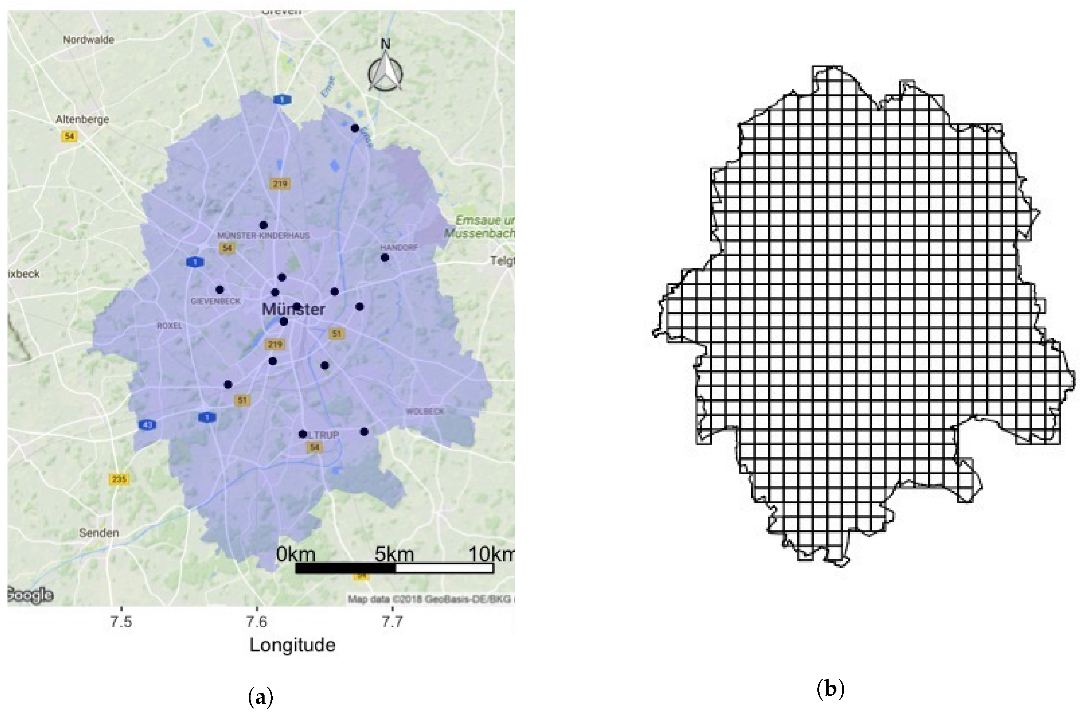
The method was applied to the city of Münster in North Rhine Westphalia, Germany (51.96 N, 7.63 E). Münster is one of the 42 agglomeration areas and one of Germany’s biggest cities in terms of area (303 km), as shown in Figure 1a. The city is divided into six administrative districts with nearly half the city’s area being agricultural, resulting in a low average population density of approximately 900 inhabitants per km, but with a population density of about 10,000 inhabitants per km in the city centre. For analysis, the whole city is divided into 599 grid cells of 1 km, as shown in Figure 1b.
As often happens for a mid-sized city in Europe, air quality data are collected by only two monitoring stations for the whole study area [20], and this is clearly insufficient for performing any meaningful geostatistical analysis. Moreover, various other air quality models such as CHIMERE, LOTOS-EUROS, and ENSEMBLE models [39] for retrieving air quality data were not very helpful, because the resolution of these models were meagre compared to the area of study. We can only represent nine cells of these standard models output for our area of interest (as shown in Figure 2). Since the data were not available for more than two monitoring stations in Münster, we added 14 simulated locations as existing air quality monitoring locations in the MND during the study. The simulation of these 14 locations was based on the argument of Ryan and LeMasters [37] for considering different land use types, and a special focus on populated areas in city (see Figure 1a and Figure A1). We assume that the knowledge about selected LUR in the study can represent the actual state of the concentration in the study area and hence predictors selected in the regression can be used to judge the performance of the proposed optimisation method.
In recent years, LUR has been a choice for various epidemiological and health studies to explain exposure [9]. In addition, this method demonstrates a better or an equivalent performance to other geostatistical methodologies such as kriging and conventional dispersion models [35]. The structure of the LUR method varies depending on the study objective and available data (i.e., number of variables, different distances and buffer sizes) due to location and size of the areas (i.e., city, state, and nation). In any case, a model typically involves information about traffic, road type & length, land use, and population. LUR uses multiple linear regression to derive the relation between air pollutant concentration and known variables at a location or its surroundings. It is then applied to unmeasured locations to predict a spatially resolved average air pollution values. The regression model is of the form :
where
- y is an n × 1 vector of air pollution concentration from monitoring sites at any particular time (in our case annual mean concentration at monitoring stations);
- X is an n × k matrix with observations of k independent variables for the n available air pollution monitoring stations;
- is a k × 1 vector of unknown parameters that we want to estimate; and
- is an n × 1 vector of errors, assumed to be independent and identically distributed.
The main strength of LUR is the empirical structure of the regression mapping and its relatively simple input/low cost (compare to dispersion modelling). A well established study for LUR model, European Study of Cohorts for Air Pollution Effects (ESCAPE), has been applied to develop local LUR models for 36 European regions for NOx, and nitrogen dioxide () [19] to explain the impact of long term exposure of air pollution on health. Methods were also hypothesised to improve the accuracy and prediction power of the LUR models using various approaches such as random forests [40]. However, the number and distribution of monitoring sites to build LUR models were identified as one of the critical factors affecting the quality of LUR outcomes in previous studies [38]. Various methods were adopted in the recent past which can help in determining the number and distribution of monitoring sites [29,31]. Few previous studies also evaluated the impact of the number of monitoring sites on LUR model results [41,42], but the influence of the spatial distribution of monitoring sites remains poorly understood. Since monitoring stations cannot be placed everywhere, the monitoring network must be used in a way that it represents critical pollutant levels where there are no monitoring stations. A viable alternative to address the constraint of monitoring station data availability could be to consider the spread of predictor variables which are available for all the locations in study area for identifying the optimal locations which can help in improving LUR robustness.
For our study, a LUR model was selected, assuming it represents annual average for the study area, pursuing the standardised predictors selected from the ESCAPE study [19]. GIS analyses were conducted to derive the discrete values of predictors at all potential monitoring station locations included in this study based on the selected LUR model. The predictor values were derived using the open geospatial data gathered from various sources, e.g. road network and building datasets were obtained from OpenStreetMap [43]. These datasets were used to calculate the total length of major roads, minor roads and building counts in varying buffers sizes of 25, 50, 100, 300, 500, 1000, and 5000 m. We also calculated the distances to the nearest major or minor roads data for each monitoring location. The city council of Münster provided traffic intensity data on major roads. Minor roads traffic intensity was calculated by spreading the 25% of the total vehicles in the city based on its length. CORINE land cover data of 2012 were used to extract the land use information around the monitoring station in the buffers. The land cover classification from CORINE was regrouped into high-density residential land, low-density residential land, industry, port, urban green, semi-natural and forest areas. We calculated the surface area of each land use regrouped in each buffer considered in the study. After model selection, predictors involved (Table 1) were further utilised in the study for identifying the combination of optimal locations for air pollution monitoring network.
4. Method
Our knowledge of air pollution monitoring is largely based on limited data. The present paper takes a new look at MND using a new optimisation method which identifies the potential locations in the study area. The optimisation methods were developed to identify the new MNDs by random perturbation over potential locations, considering associated predictors within the LUR models. The random selection of the monitoring sites, and the optimisation of their spatial distribution in the study area was implemented using Spatial Simulated Annealing (SSA).
4.1. Spatial Simulated Annealing (SSA)
Having an objective before initiating the monitoring campaign is helpful in distributing the sensors optimally. The objective must be in agreement with the aim of the study. If the objective requires monitoring the excess level of pollutants, one approach is to locate the monitoring sites in the study area where pollutants concentration is higher. Usually, such design of the network is in agreement with the intention to monitor the maximum exposure values, and it does not represent the whole picture about the air pollution in the city. Air quality varies on a comparatively small scale, as the pollutant concentration at a particular place relies heavily on local emission sources, structures and atmospheric flow conditions [22,44,45]. The location selection for MND can be optimised numerically using approaches such as geostatistical surveys, where probability sampling is not considered [46]. Finding the optimal locations for monitoring networks manually is practically impossible given the extraordinary number of possible combinations, even with the coarse grid than we considered for our study. This process can be automated by using the spatial numerical search algorithm called spatial simulated annealing (SSA). The method implements optimisation by generating a sequence of new possible monitoring locations. A new monitoring location is considered by selecting random locations and shifting them in a random direction over the random distance in two dimensional space defined in the optimisation process. After each such perturbation, the mismatch between the current MND’s discrete value and the observed new MND’s value is quantified for combination of locations according to a predefined optimisation criterion function. In the 2000s, van Groenigen [32] introduced a simulated annealing algorithm as a method to find the spatial distributions of monitoring points based on an optimisation criterion function. Over the years, the approach has been used for investigating optimal sample designs for criterion as variogram estimation [47], thinning existing sampling networks [48], optimisation of geostatistical surveys [49], phased sampling designs for containment urban soil [50], and Kriging with External Drift (KED) variance minimisation for rainfall prediction [51], to name just a few.
The SSA approach to finding an optimal monitoring design involves the minimisation of the optimisation criterion value using an objective function such as the average kriging variance across the area of interest [32]. The optimal location identification problem is formalised as a single-objective optimisation function, pointing at criteria involving discrete-valued variables. For some monitoring design objectives, the optimality of a particular combination of monitoring sites may be judged based on more than one criterion, considering not only the quality of the resulting information obtained but also the cost of acquiring the data.
4.2. Optimisation Criterion Estimation
The optimal MND is the configuration for which the criterion chosen is minimal. The criterion we used in this study is to minimise the spatial mean prediction error for the selected LUR model. Under the assumption of independent and identically distributed (IID) errors, the (ordinary least squares) estimator of is a linear combination of the observations y:
and the predicted pollutant concentration for a new location with predictor variables is given by
with the k × 1 vector with predictor variables at that location.
The estimation error in is
and hence the error in is
with the variance of .
Considering a two-dimensional study area A, we want to decrease the prediction error using n observation sites using a network design . The optimisation process starts with a existing MND (can also be done using randomly selected monitoring design) , consisting of observation points with corresponding predictor variable vectors , …, . At the first optimisation step, the monitoring sites are transformed into a random vector with only one element different from the initial, yielding a new monitoring design . During the optimisation process, the prediction error is calculated at each node of the rasterised study area A.
The different monitoring sites in the MND are supposed to cover a diverse range of representative areas. Therefore, to optimise the MND considering all the sites in MND, we average over all potential locations inside the study area A. Since acts as a constant, we leave it out and use as criterion:
with the size of the area (expressed as the number of grid cells representing the area). In this optimisation criterion, manipulating the MND leads to the modification of X.
The typical aim for air pollution monitoring is to accurately measure air quality and understand the impact of ambient air pollution on population. However, because of the limited number of possible monitoring station sites, we need to prioritise the MND optimisation in a way that it can help in collecting precise information about air quality in the residential area of the cities. With this aim, we fine tuned the above mentioned optimisation method to identify the optimal locations which can help in decreasing the spatial mean prediction error prioritising areas where the population resides. This newly extended optimisation criterion can be written as:
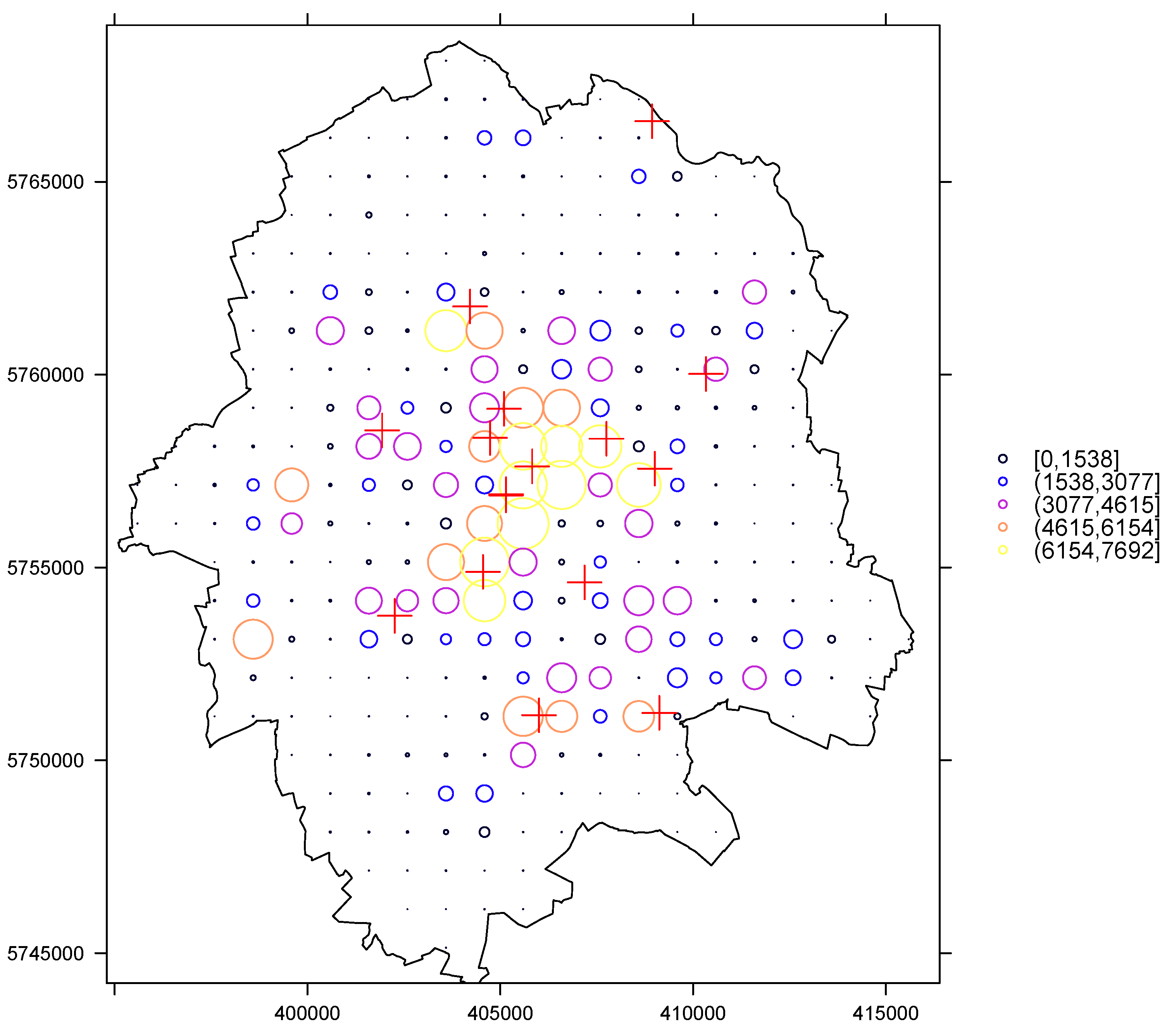
where is the population at location . We established the weight for our study by focusing on the areas with more than 1500 houses per grid cells (see Figure A1 in Appendix A).
We use as scenario a setting where (due, e.g., to budget and infrastructure constraints) the number of air quality monitors deployed n are fixed. We aim to find the optimal locations for the specific n monitors, which can help in developing the robust LUR model for cities. The optimisation method developed in this section will allow us to compare the different possible combinations for optimal MND. In this study, we only consider a static design for the monitoring network, i.e., locations of the network do not change over time. With a finite number of candidate locations N derived by discretising the whole study area A, we can get combinations, and select the one which minimises the optimisation criterion. Every time a new possible MND is generated, the optimisation criterion mentioned earlier is calculated and compared with the criterion value of the previously selected monitoring design. The new location will be accepted if the MND leads to a smaller optimisation criterion overall. If the MND leads to a larger optimisation criterion, the new design might sometimes be accepted, based on the probability of acceptance defined in the parameters of the annealing algorithm, expressed as:
where is a control parameter which controls the number of remaining iterations. The temperature defined in the annealing algorithm decreases from a positive starting value to zero as the count of iterations increases. From Equation (8), we see that, at a given temperature, the larger the increase in criterion value, the smaller will be its probability to accept a worse network design. In addition, for lower values for temperature (at larger number of iterations), the probability of accepting a worse design becomes lower. The repetition for a new design creation continues until the total number of defined iterations has been achieved. We refer to the work of Heuvelink et al. [52] for a more detailed explanation of the optimisation algorithm used in our study.
4.3. The Optimisation Procedure
The steps of the optimisation algorithm are the following:
- A LUR model is chosen for the study area by selecting predictors that explain the air pollutant considered.
- An initial (possibly existing) monitoring design is defined, consisting of n observations to be optimised.
- The area of study A is discretised, the raster is defined with N raster nodes.
- is modified, returning a monitoring design and the new mean prediction error is calculated
- A new monitoring design is accepted if it reduced the optimisation criterion value or rejected as the basis for further optimisation based on Equation (8).
- The optimisation continues until the proposal monitoring designs are no longer accepted, based on energy transition and iteration parameters.
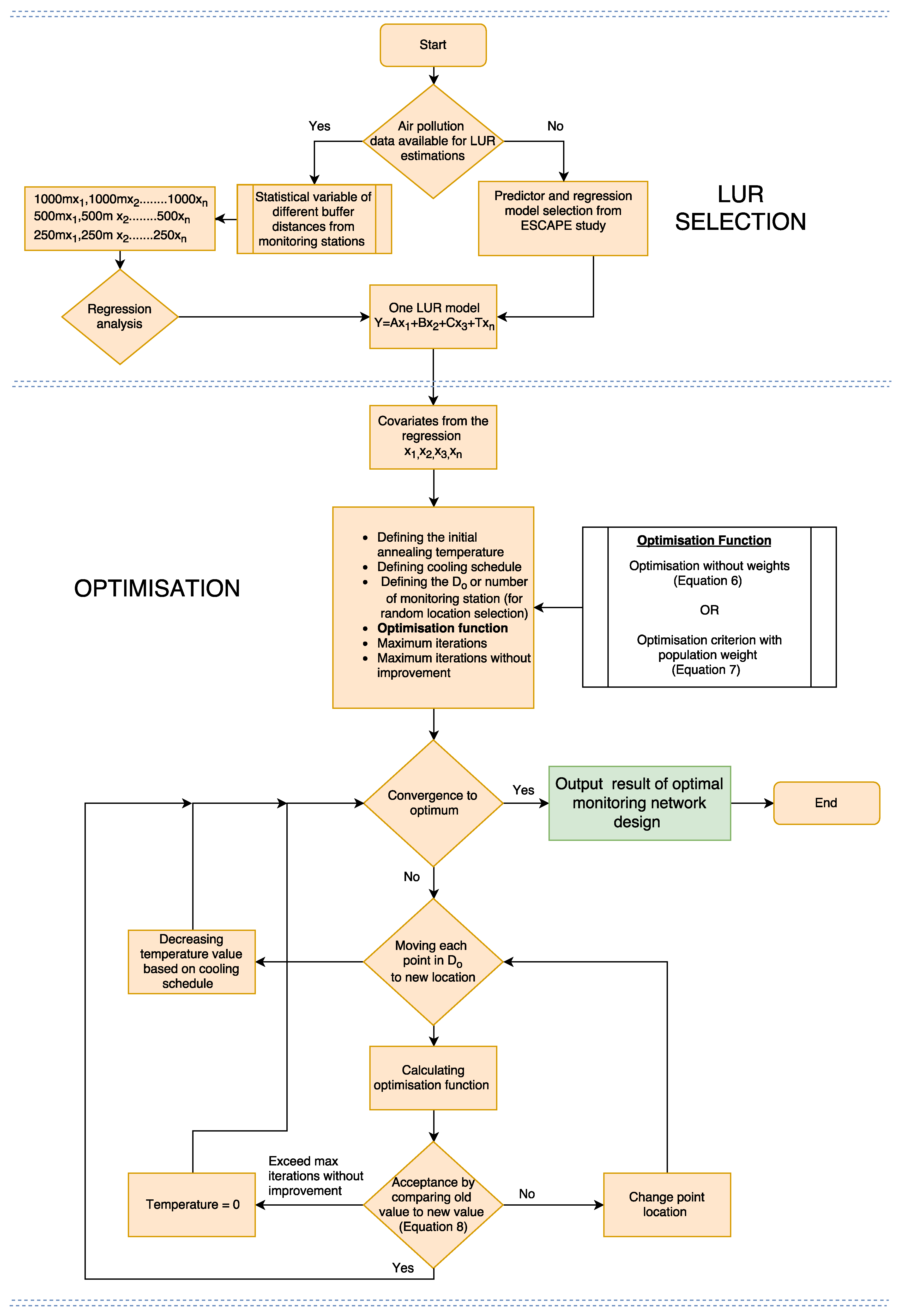
The schematic overview of the proposed optimisation method described above is shown in Figure 3. All geospatial and statistical calculations for the study were conducted using the R packages sp [53], sf [54]. For running SSA, we used the R package spsann [55]. The source code for the proposed optimisation method can be accessed from Github [56].
5. Results
Nine (out of 58) predictor variables were used from the selected LUR model (Table 1). The variables were selected based on the existing knowledge about their relationship with the pollution concentration data and their inclusion in previous LUR models [19]. We used all 599 raster cell as the potential locations for monitoring stations and the associated values of selected predictors at those locations in SSA to find the optimal MND. The inputs for running both of our optimisation algorithms require a raster grid with potential sites (599 cells) for monitoring stations, the predictor of the LUR as covariates for each raster cell, an initial monitoring network design with the location of existing monitoring stations, the temperature and the probability of acceptance parameters for annealing.
5.1. Optimisation without a Weighted Function for the Study Area
The optimal MND identification started with monitoring network points, based on already existing monitoring network design (). The method iterated to select any MND which can minimise the criterion value recognising the optimisation method (Equation (6)), and representing a minimum spatial mean prediction error for the study area. Figure 4 represents the criterion values achieved at different probability parameter values while keeping other annealing parameters constant during the whole process. Figure 5 shows that several worsened designs were accepted in the beginning, succeeding that the mean prediction error steadily decreased. After about 3500 iterations, no substantial further reduction was achieved, indicating that the algorithm reached a nearly optimum configuration design, as was confirmed by observing the similar patterns of decline at different runs. Overall, the defined criterion was considerably dropped from 156.5 to 0.1918595 with 0.3 as probability of acceptance, which shows an improvement of about 99.87%.
It can be inferred from the results in Figure 6 that the final optimised monitoring locations have a larger density around the city centre than in the initial monitoring design, and this is consistent with the population-based optimisation criterion for MND defined earlier.
5.2. Optimisation with a Population Weighted Function for the Study Area
After realising the optimal MND that represents the least spatial mean prediction error for the study area, we considered focusing on the areas with high population density (calculated based on the number of residential buildings around each potential location for the monitoring stations). Equation (7) was used as a criterion for implementing the weighted optimisation method.
Again, the configuration was considered optimal based on the least energy (spatial mean prediction error) obtained during the calculation of the criterion value at various probabilities (Figure 7). Figure 8 shows the optimised monitoring design obtained after running the algorithm. As a comparison with Figure 6b, an alternative design was obtained using the weighted spatial areas of highly populated housing areas (see Figure A1). The new monitoring design has a close resemblance to the previous optimal configuration but this time with more emphasis on the area with weight (green areas in the Figure 8b represents populated housing areas) than on areas with no weight (or non-housing areas). The optimised MND represents a significant drop in the spatial mean prediction error, from 571,492.23 to 332.8651, a difference of about 99.94%. The optimal configuration obtained at various other probability of acceptance presented graphically can be found in Appendix C. The optimised monitoring networks also placed the monitor locations towards the boundary of the study area. This is a well-known effect while running SSA, expressed by van Groenigen [32] in the literature.
5.3. Sensitivity of the Optimisation Methods
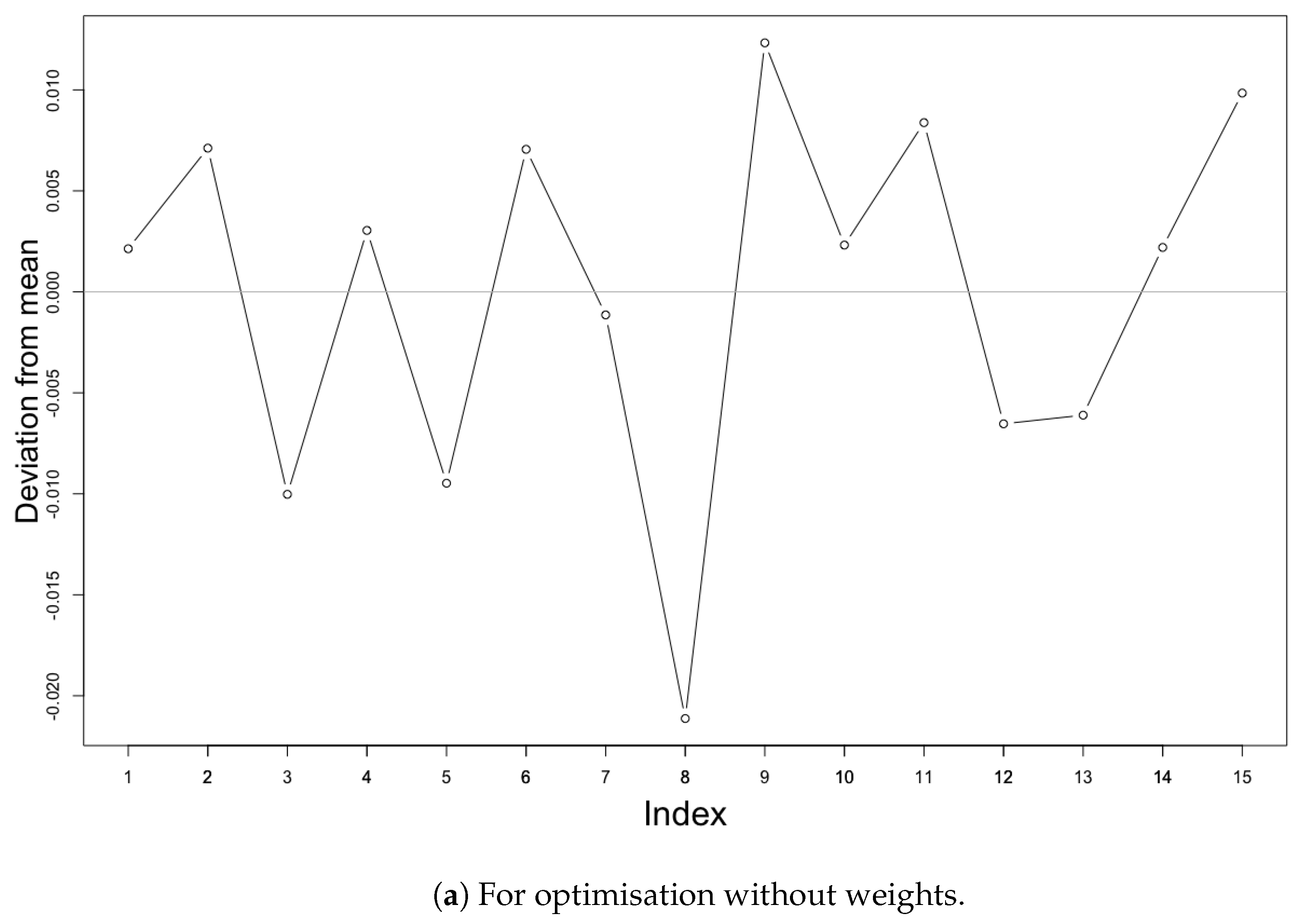
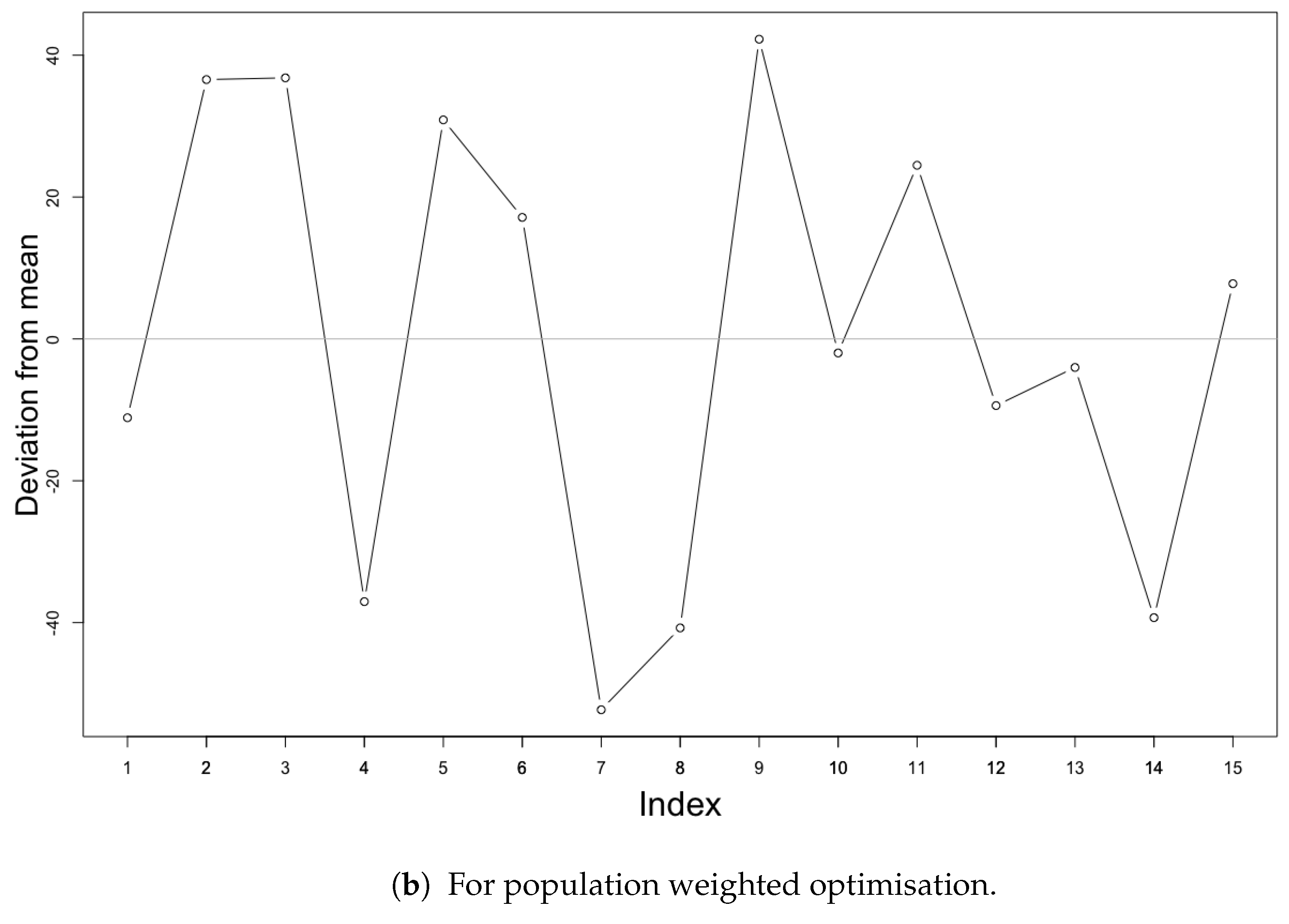
The distribution of optimal monitoring sites at various locations and its criterion values can be influenced by various parameters or with different iterations. Indeed, SSA is a stochastic algorithm and does not generate a unique spatial distribution of monitoring stations at each run (i.e., algorithm execution). To investigate the variation in final criterion values for each complete process of optimisation, we ran the algorithm 15 times each for both without weighted optimisation and with population weighted area optimisation. The 15 runs for each involve exactly the same parameters and the probability of acceptance as the run with the least optimisation criterion values according to the graphs of previous runs (see Figure 4 and Figure 7) (i.e., 0.3 probability of acceptance for non weighted and 0.1 probability of acceptance for weighted area, respectively). Figure 9 shows the results of the investigation for change in optimal criterion values. The resulting energy state for the optimisation criterion without weights returned values with mean 0.2058 and standard deviation of 0.0091 or 4.42%. In the case of the population-weighted optimisation run, the criterion values obtained were with the mean of 398.030 and standard deviation of 31.53 or 7.3%. These small deviations from the mean values can be considered as insignificant in comparison with the improvement of around 99% in spatial mean prediction error for both the methods.
Besides the variation of final criterion values per run, the sensitivity of our method to the number of monitoring stations in the optimisation method was also investigated. For this, we changed the numbers of monitoring sites in the input parameters. Figure 10 compares the criterion value obtained at a different monitoring station involved in the optimisation method. We again used the same optimisation method parameters with the least criterion values of 0.3 and 0.1 probability of acceptance from the results obtained in previous runs (Figure 4 and Figure 7) for this investigation. More monitoring stations yielded better results; the spatial mean prediction error decreased with a increase in monitoring sites. However, we kept other parameters such as initial temperature, chains and temperature change for all the optimisation runs unchanged. It would be interesting to investigate the influence of the change in parameters and number of monitoring stations on the outcome of the optimisation method.
5.4. Comparative Analysis
From the above results, we can infer that the combinations of locations obtained from our optimisation methods employed in the selected study area give satisfactory results towards the development of a reliable, less assumption based, less data intensive, easy to use and low-cost methods for identifying the optimal location for air quality monitoring at a city level. The proposed methods also consider the enhanced efforts to anticipate areas of more importance (such as residential areas) in cities for planning air pollution monitoring network, without using pollutants monitoring station values as inputs. Since LUR have been a useful exposure estimation method in various epidemiological and public health studies. Location optimisation considering such methods can be useful to understand exposure in cities. At this point, it could be useful to compare the results of the proposed methods with results from previous similar research works [27,28,29,33,34,38], where other strategies were adopted to identify the optimal locations for air quality MND. The main difference with these approaches is that the proposed optimisation method used LUR predictor variables values which are available for all the candidate locations of the study area for optimal location identification, rather than the computationally intensive datasets inputs from dispersion models (which sometime are not accessible at the city level). The proposed method tries to address the fundamental input data required for air quality monitoring initiatives with the significant decrease in the assumption parameter involvement in the previous studies (such as dispersion model or emission sources and its assumptions) for location optimisation. In addition, the proposed method is more flexible and low cost compared to others, as it uses the easily accessible geospatial data for LUR estimation. The approach is also less data intensive compared to other existing approaches for optimal design of MND [28,33,34]. Moreover, few of the methods in the literature are suitable for application on a smaller scale, such as cities, because of spatial resolution limits of the input datasets [29,38]. As illustrated in Section 5.2, the current method does not suffer from this drawback, and is applicable at the city level.
6. Discussion
In this paper, we have presented an optimisation method that can help identifying the optimal MND for robust LUR estimations. The method utilises the predictors selected in the regression model for optimal location identification. The optimisation method shown in this study was initially developed to select the combination of locations which can represent the least spatial mean prediction error in air pollution estimation without giving weights to any specific regions in the study area. Figure 6 presented the outcome obtained by applying this optimisation method. Furthermore, to consider the relevance of precise air pollution information close to population, the initial optimisation method was further adapted to prioritise the specific regions of importance in the study area. The weights for the population were added to the optimisation method for identifying the optimal combination of locations that minimise the spatial mean prediction error while prioritising populated regions in the study area. SSA was used to implement the optimisation. Figure 8 showed the results of the modified optimisation method for the study area. Overall, the proposed approach can be of interest to air quality management authorities, researchers trying to monitor the air pollution, particularly if considering LUR estimation methods, and to the city councils to better collect air quality data in future. As discussed in Gupta et al. [57], it has the potential of addressing big data challenges in environmental monitoring. The method can also be of use in other domains, such as sound pollution studies, which also utilise land use regression estimations.
The standard criteria used for ambient air quality assessment are the number and locations of monitoring stations. The number of monitoring stations and locations affects the degree of detail for pollution monitoring across regions. According to the EU directive of 2008 [20], a minimum of one monitoring station per million inhabitants over agglomerations and additional urban areas of more than 100,000 inhabitants is required for placing air quality monitoring stations. A large number of EU member states seems to follow the strict minimum regarding number of monitoring stations, and this leads to a low resolution air quality data inventory for cities. Previous work has shown that using a limited number of monitoring stations in cities will not be sufficient for determining the patterns of air pollutants due to their complex behaviour [31]. Given that the collection of ambient air quality data is not possible at all locations in the study area, optimising the distribution of monitoring stations can help in collecting precise representative information for all the locations in the study area.
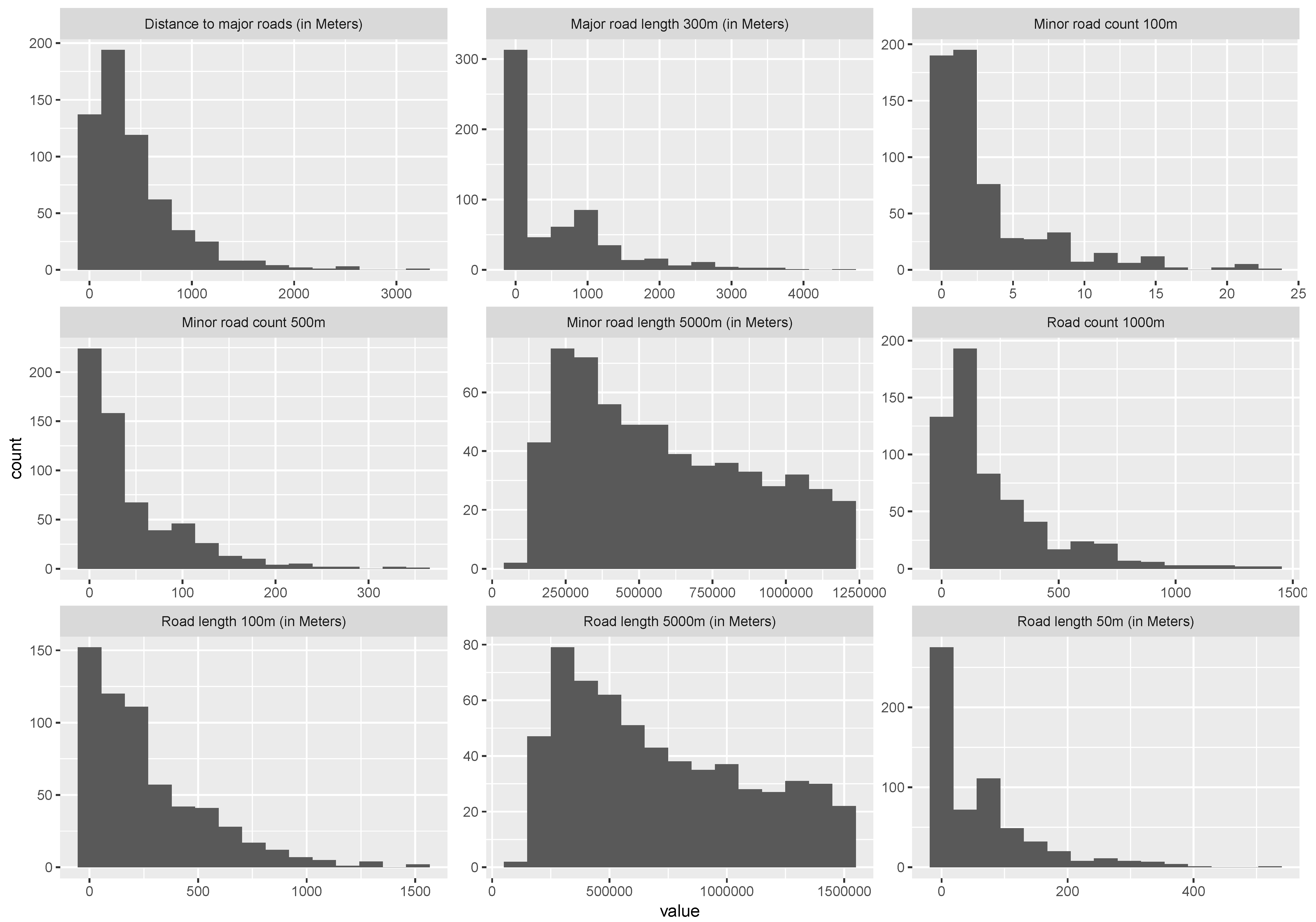
Randomly selecting monitoring station locations in the area could result in a clustered or dispersed design which may be ineffective and not representative for the real aim of the study. The efficiency of spatial monitoring design can be increased by embedding prior knowledge about the random field [58]. According to [28], the design of monitoring network involves three significant considerations: (1) determining the design criteria; (2) estimating the concentration of pollutant; and (3) solving an optimisation problem. The proposed optimisation methods favour all three considerations. Firstly, it takes into account the design criterion which focuses on identifying the combination of locations for decreasing the spatial mean prediction error in the area. Secondly, the selection of MND in the optimisation method is dependent on the linear function of predictors which estimate air pollution concentration. The optimal design will decrease the error for the estimated air pollution values based on predictors involved in the optimisation process. Figure A2 in Appendix B shows the histograms of various predictors used in the present optimisation study. It is worth mentioning here that the selection of predictors for optimisation may differ from those considered in the ESCAPE study if real data about monitoring stations is available or the number of monitoring stations involved in the initial monitoring design () changes for area-specific LUR estimations. Lastly, the proposed optimisation methods in the current study can help in solving the problem for robust LUR estimation for the study area by identifying the optimal location underlying the specific LUR model. The weight-based optimisation method also supports solving the optimisation problem based on a specific goal of the study by prioritising specific regions in the study area. The final optimal MNDs obtained from the proposed optimisation method were successful in selecting a combination of the broad range of locations (such as roads or residential areas) while also giving higher priority in the area-weighted optimisation. Thus, we complement the finding of Wu et al. [38] regarding the advantage of mixed site MND for LUR exposure analyses.
This study optimised MND by minimising the spatial mean prediction error while using a given LUR model. To the best of our knowledge, such an approach has not been used before concerning LUR based air quality monitoring network optimisation. It is essential to find the optimal locations for the case of future monitoring campaigns plans to readjust the existing network or to develop a new MND for the city. The two significant advantages of the proposed optimisation method are: (1) flexible covariate integration, which allows the integration of other possible variables of interest for optimisation; and (2) autonomy to monitoring data, hence avoiding dependencies on monitoring data for identifying locations for MND. Overall, the flexibility offered by the proposed methods can be helpful in developing the optimal MND for the area with no or negligible amount of air pollution monitoring data. Furthermore, we would like to emphasise that this method only applies to optimisation of the MND based on an already selected LUR model. In case of unavailability of air pollution monitoring data for estimating LUR, various already existing standard LUR models (e.g., ESCAPE [19]) regression models can be considered for optimising the MND as we did in our study. This particular advantage can help in setting up the air pollution monitoring network from a very early stage for underlying a selected LUR model. Another significant advantage of the proposed methods can be to overcome the limitation of the LUR models concerning transferability. According to Hoek et al. [35], transferability of LUR models depends on the similarity of the area regarding land use. On the other hand, Johnson et al. [59] stated that LUR models are not transferable most of the time. With the help of the proposed method, it is possible to initiate air quality monitoring considering the specific LUR of interest hence making it transferable. Based on the study focused on transferability by Allen et al. [60], it was suggested that locally calibrated models performed better than the transferred model. The proposed method can be used as a tool for transferring the selected model and re-calibrating it locally by optimising the locations of monitoring station using predictors. Furthermore, the method provides resilience for increments and decrements of weights as per the aim for distribution of monitoring sites.
Limitations and Future Work
There are also limitations to the proposed method. First, the selection of a LUR model is vital for implementing the optimisation method, which means that, in the case of unavailability of monitoring station data for LUR model estimation, the regression model needs to be assumed from previous studies. In this case, the selection would be arbitrary, and may not provide a correct representation of the air pollution variability in the area of study. The availability of data and selection procedures for predictors selection in regression model also impacts the outcome. Second, the underlying assumptions of multiple regression concerning linearity between dependent and independent variables in the regression, independence and normal distribution of error term may create bias in the interpretation of the final results, which are the typical limitations for many simplistic LUR based studies. Third, the initial MND () considered in the study is comprised of 16 monitoring stations, of which 14 locations are simulated, and 2 originally had a known location. These two stations, in reality, will not be considered for relocation easily based on various objective functions. Further research should be dedicated to fine tune the existing criterion functions which can restrict perturbation of permanently located monitoring stations but only allowing optimal location identification for additional monitoring stations [32]. These limitations also highlight the difficulty of having proper data about air pollution and concerning predictors. There may also be several other sources which can inherit errors, concerning the open data and simulated locations of monitoring stations used in the study. Although many optimisation methods have already been developed, the flexibility offered by our method provides room for more insights to be considered for optimisation in the future. For example, taking into account the geographical information, preliminary observations, and information on the spatial correlation could have helped in improving MND optimisation strategy [49,51,61]. We have not considered using such optimisation constraints in the current study, but they could be integrated during future research.
Future work will include the testing of the method with other datasets in different cities. As to the potential of low-cost sensors to increase the spatial coverage of air pollution monitoring (which has been a matter of discussion in recent years, see [62]), the proposed method can be further extended for decisions making process about where one should deploy low-cost sensors for air pollution monitoring in cities. Further data collection is required to determine precisely how air pollution monitoring network can be developed and optimised considering various LUR models for higher resolution air pollution monitoring in the study area. Further studies can also be carried out, utilising enhanced data collection procedures including systemic crowd-sourcing approaches and higher resolution remote sensing data from the various missions (such as Sentinel-4 and -5P), to enable air pollution monitoring efforts at the higher spatial scale in cities. Thus, encouraging the efficient monitoring of air pollution distribution and gathering information about the possible exposure of the population can serve as a base for improving environmental sustainability and urban health.
7. Conclusions
LUR models provide the opportunity to take into account within-city variability of air pollution concentration for epidemiological and public health studies. In the present study, we aimed at improving the robustness of LUR by identifying the combination of locations which can decrease the spatial mean prediction error for air quality estimation in the cities. A statistical optimisation method was developed to optimise locations in the study area. The initial version of the optimisation method focused on identifying the locations for MND which can help in representing the air pollution estimates with minimal spatial mean prediction error considering an area of interest. This version was then further modified to include the weighted function of the population to determine optimal locations which can represent the estimates with least spatial mean prediction error in high density populated spaces of the study area. The methods require all predictor variables in selected LUR to be known at all of the potential locations for calculating their significance in the optimisation process. The optimisation method does not rely on monitoring station data for monitoring site placement, thus giving independence for planning and readjustments of the optimal air quality MND for the cities with no or insignificant amount of air quality data. Furthermore, we demonstrated that, by distinguishing between weighted areas, the optimisation method could be a helpful tool in air quality monitoring and exposure studies. The proposed optimisation method is an efficient way to achieve air quality estimates with minimal prediction errors to understand air pollution variability and support the sustainable air quality control efforts for the urban spaces. One possible extension of the method could be the inclusion of Wu and co-workers’ work on selecting the number of monitoring stations required and their optimal design for robust LUR estimation. Moreover, the possibility to prioritise particular areas of interest may be considered as a useful control in the air quality control and exposure assessment related decision-making processes. Additional further work could include assessing how the method performs when provided with various quality of LUR models and data sources for a given urban area as input.In all, the proposed optimisation method can be a helpful tool in air quality MND that enables LUR estimations with fewer errors for preventing air pollution exposure and advancing urban health sustainability.
Author Contributions
S.G. and E.P. conceived the optimisation method. S.G. developed and performed the main proportions of the study. E.P. and J.M. provided advice regarding the optimisation method and performance. A.D. supported in shaping the presentation of the paper.
Acknowledgments
The authors gratefully acknowledge funding from the European Commission through the GEO-C project (H2020-MSCA-ITN-2014, Grant Agreement Number 642332, http://www.geo-c.eu/).
Conflicts of Interest
The authors declare no conflict of interest.
Abbreviations
The following abbreviations are used in this manuscript:
| MND | Monitoring Network Design |
| LUR | Land Use Regression |
| ESCAPE | European Study of Cohorts for Air Pollution Effects |
| OECD | Organisation for Economic Co-operation and Development |
| WHO | World Health Organisation |
| PM | Particulate Matter |
| EC | Elemental Carbon |
| Ozone | |
| CORINE | coordination of information on the environment |
Appendix A
This section contain the map of the study area to represent the spread of data populated housing areas.
Figure A1.
Populated housing area map with initial monitoring station locations (red plus signs) for study area.
Figure A1.
Populated housing area map with initial monitoring station locations (red plus signs) for study area.
Appendix B
The following image shows the histogram of all the predictor variables used in the study as described in Table 1.
Figure A2.
Histogram of predictor variables for LUR used in the study.
Appendix C
In this section, we show all the configurations we realised for the study area by using optimisation method for non weighted and weighted optimisation.

Table A1.
All the configuration realised for optimisation at different probability of acceptance.
| Various other configurations realised during the study for different probability of acceptance | |
|---|---|
| Without weight optimisation | Population weighted optimisation |
 |  |
| Spatial mean prediction Error: 0.1990 | Spatial mean prediction Error: 404.57 |
 |  |
| Spatial mean prediction Error: 0.2039 | Spatial mean prediction Error: 363.34 |
 |  |
| Spatial mean prediction Error: 0.21179 | Spatial mean prediction Error: 332.86 |
 |  |
| Spatial mean prediction Error: 0.2018 | Spatial mean prediction Error: 370.25 |
 |  |
| Spatial mean prediction Error: 0.1918 | Spatial mean prediction Error: 385.52 |
 |  |
| Spatial mean prediction Error: 0.2027 | Spatial mean prediction Error:405.39 |
 |  |
| Spatial mean prediction Error: 0.2579 | Spatial mean prediction Error: 387.15 |
 |  |
| Spatial mean prediction Error: 0.2043 | Spatial mean prediction Error: 387.57 |
 |  |
| Spatial mean prediction Error: 0.19381 | Spatial mean prediction Error: 27798.28 |
 |  |
| Spatial mean prediction Error: 0.2094 | Spatial mean prediction Error: 333.96 |
References
- United Nations. World Urbanization Prospects: The 2014 Revision, Highlights. Department of Economic and Social Affairs; Population Division; United Nations: New York, NY, USA, 2014. [Google Scholar]
- Marchal, V.; Dellink, R.; Van Vuuren, D.; Clapp, C.; Chateau, J.; Magné, B.; van Vliet, J. OECD Environmental Outlook to 2050; Organization for Economic Co-operation and Development: Paris, France, 2011. [Google Scholar]
- Zivin, J.G.; Neidell, M. Air pollution’s hidden impacts. Science 2018, 359, 39–40. [Google Scholar] [CrossRef] [PubMed]
- Cohen, A.J.; Brauer, M.; Burnett, R.; Anderson, H.R.; Frostad, J.; Estep, K.; Balakrishnan, K.; Brunekreef, B.; Dandona, L.; Dandona, R.; et al. Estimates and 25-year trends of the global burden of disease attributable to ambient air pollution: An analysis of data from the Global Burden of Diseases Study 2015. Lancet 2017, 389, 1907–1918. [Google Scholar] [CrossRef]
- Fugiel, A.; Burchart-Korol, D.; Czaplicka-Kolarz, K.; Smoliński, A. Environmental impact and damage categories caused by air pollution emissions from mining and quarrying sectors of European countries. J. Clean. Prod. 2017, 143, 159–168. [Google Scholar] [CrossRef]
- Zhang, Q.; Jiang, X.; Tong, D.; Davis, S.J.; Zhao, H.; Geng, G.; Feng, T.; Zheng, B.; Lu, Z.; Streets, D.G.; et al. Transboundary health impacts of transported global air pollution and international trade. Nature 2017, 543, 705. [Google Scholar] [CrossRef] [PubMed]
- WHO. Global Platform on Air Quality and Health. Available online: http://www.who.int/phe/health_topics/outdoorair/global_platform/en/ (accessed on 1 May 2018).
- Jerrett, M.; Arain, M.A.; Kanaroglou, P.; Beckerman, B.; Crouse, D.; Gilbert, N.L.; Brook, J.R.; Finkelstein, N.; Finkelstein, M.M. Modeling the intraurban variability of ambient traffic pollution in Toronto, Canada. J. Toxicol. Environ. Health Part A 2007, 70, 200–212. [Google Scholar] [CrossRef] [PubMed]
- Khreis, H.; Kelly, C.; Tate, J.; Parslow, R.; Lucas, K.; Nieuwenhuijsen, M. Exposure to traffic-related air pollution and risk of development of childhood asthma: A systematic review and meta-analysis. Environ. Int. 2017, 100, 1–31. [Google Scholar] [CrossRef] [PubMed]
- McConnell, R.; Islam, T.; Shankardass, K.; Jerrett, M.; Lurmann, F.; Gilliland, F.; Gauderman, J.; Avol, E.; Künzli, N.; Yao, L.; et al. Childhood incident asthma and traffic-related air pollution at home and school. Environ. Health Perspect. 2010, 118, 1021. [Google Scholar] [CrossRef] [PubMed] [Green Version]
- Health Effects Institute. Panel on the Health Effects of Traffic-Related Air Pollution. Traffic-Related Air Pollution: A Critical Review of the Literature on Emissions, Exposure, and Health Effects; Number 17; Health Effects Institute: Cambridge, MA, USA, 2010. [Google Scholar]
- Charpin, D.; Caillaud, D.M. Air pollution and the nose chronic respiratory disorders. In The Nose and Sinuses in Respiratory Disorders ERS Monograph; European Respiratory Society: Polymouth, UK, 2017; Volume 76, p. 162. [Google Scholar]
- Mayer, H. Air pollution in cities. Atmos. Environ. 1999, 33, 4029–4037. [Google Scholar] [CrossRef]
- Conti, G.O.; Heibati, B.; Kloog, I.; Fiore, M.; Ferrante, M. A review of AirQ Models and their applications for forecasting the air pollution health outcomes. Environ. Sci. Pollut. Res. 2017, 24, 6426–6445. [Google Scholar] [CrossRef] [PubMed]
- Bougoudis, I.; Demertzis, K.; Iliadis, L.; Anezakis, V.D.; Papaleonidas, A. FuSSFFra, a fuzzy semi-supervised forecasting framework: the case of the air pollution in Athens. Neural Comput. Appl. 2018, 29, 375–388. [Google Scholar] [CrossRef]
- Bougoudis, I.; Demertzis, K.; Iliadis, L. Fast and low cost prediction of extreme air pollution values with hybrid unsupervised learning. Integr. Comput.-Aided Eng. 2016, 23, 115–127. [Google Scholar] [CrossRef]
- Feng, X.; Li, Q.; Zhu, Y.; Hou, J.; Jin, L.; Wang, J. Artificial neural networks forecasting of PM2. 5 pollution using air mass trajectory based geographic model and wavelet transformation. Atmos. Environ. 2015, 107, 118–128. [Google Scholar] [CrossRef]
- Briggs, D. The role of GIS: Coping with space (and time) in air pollution exposure assessment. J. Toxicol. Environ. Health Part A 2005, 68, 1243–1261. [Google Scholar] [CrossRef] [PubMed]
- Beelen, R.; Hoek, G.; Vienneau, D.; Eeftens, M.; Dimakopoulou, K.; Pedeli, X.; Tsai, M.Y.; Künzli, N.; Schikowski, T.; Marcon, A.; et al. Development of NO2 and NOx land use regression models for estimating air pollution exposure in 36 study areas in Europe–the ESCAPE project. Atmos. Environ. 2013, 72, 10–23. [Google Scholar] [CrossRef]
- European Parliament and Council of the European Union. Directive 2008/50/EC of the European Parliament and of the Council of 21 May 2008 on ambient air quality and cleaner air for Europe. Off. J. Eur. Union 2008, L 152/1–L 152/43. [Google Scholar]
- Raffuse, S.; Sullivan, D.; McCarthy, M.; Penfold, B.; Hafner, H. Ambient air monitoring network assessment guidance, analytical techniques for technical assessments of ambient air monitoring networks. Retrieved July 2007, 20, 2007. [Google Scholar]
- Ott, D.K.; Kumar, N.; Peters, T.M. Passive sampling to capture spatial variability in PM10–2.5. Atmos. Environ. 2008, 42, 746–756. [Google Scholar] [CrossRef]
- Goldstein, I.F.; Landovitz, L. Analysis of air pollution patterns in New York City—I. Can one station represent the large metropolitan area? Atmos. Environ. (1967) 1977, 11, 47–52. [Google Scholar] [CrossRef]
- Kanaroglou, P.S.; Jerrett, M.; Morrison, J.; Beckerman, B.; Arain, M.A.; Gilbert, N.L.; Brook, J.R. Establishing an air pollution monitoring network for intra-urban population exposure assessment: A location-allocation approach. Atmos. Environ. 2005, 39, 2399–2409. [Google Scholar] [CrossRef]
- Nejadkoorki, F.; Nicholson, K.; Hadad, K. The design of long-term air quality monitoring networks in urban areas using a spatiotemporal approach. Environ. Monit. Assess. 2011, 172, 215–223. [Google Scholar] [CrossRef] [PubMed]
- Kuhlbusch, T.A.; Quass, U.; Fuller, G.; Viana, M.; Querol, X.; Katsouyanni, K.; Quincey, P. Air pollution monitoring strategies and technologies for urban areas. In Urban Air Quality in Europe; Springer: Berlin/Heidelberg, Germany, 2013; pp. 277–296. [Google Scholar]
- Mofarrah, A.; Husain, T. A holistic approach for optimal design of air quality monitoring network expansion in an urban area. Atmos. Environ. 2010, 44, 432–440. [Google Scholar] [CrossRef]
- Wu, L.; Bocquet, M.; Chevallier, M. Optimal reduction of the ozone monitoring network over France. Atmos. Environ. 2010, 44, 3071–3083. [Google Scholar] [CrossRef]
- Benis, K.Z.; Fatehifar, E.; Shafiei, S.; Nahr, F.K.; Purfarhadi, Y. Design of a sensitive air quality monitoring network using an integrated optimization approach. Stoch. Environ. Res. Risk Assess. 2016, 30, 779–793. [Google Scholar] [CrossRef]
- Elkamel, A.; Fatehifar, E.; Taheri, M.; Al-Rashidi, M.; Lohi, A. A heuristic optimization approach for Air Quality Monitoring Network design with the simultaneous consideration of multiple pollutants. J. Environ. Manag. 2008, 88, 507–516. [Google Scholar] [CrossRef] [PubMed]
- Wang, K.; Zhao, H.; Ding, Y.; Li, T.; Hou, L.; Sun, F. Optimization of air pollutant monitoring stations with constraints using genetic algorithm. J. High Speed Netw. 2015, 21, 141–153. [Google Scholar] [CrossRef]
- Van Groenigen, J.W. Constrained Optimisation of Spatial Sampling: A Geostatistical Approach. Ph.D. Thesis, Wageningen University and Research, Wageningen, The Netherlands, 1999. [Google Scholar]
- Sarigiannis, D.A.; Saisana, M. Multi-objective optimization of air quality monitoring. Environ. Monit. Assess. 2008, 136, 87–99. [Google Scholar] [CrossRef] [PubMed]
- Kao, J.J.; Hsieh, M.R. Utilizing multiobjective analysis to determine an air quality monitoring network in an industrial district. Atmos. Environ. 2006, 40, 1092–1103. [Google Scholar] [CrossRef]
- Hoek, G.; Beelen, R.; De Hoogh, K.; Vienneau, D.; Gulliver, J.; Fischer, P.; Briggs, D. A review of land-use regression models to assess spatial variation of outdoor air pollution. Atmos. Environ. 2008, 42, 7561–7578. [Google Scholar] [CrossRef]
- Marshall, J.D.; Nethery, E.; Brauer, M. Within-urban variability in ambient air pollution: comparison of estimation methods. Atmos. Environ. 2008, 42, 1359–1369. [Google Scholar] [CrossRef]
- Ryan, P.H.; LeMasters, G.K. A review of land-use regression models for characterising intraurban air pollution exposure. Inhal. Toxicol. 2007, 19, 127–133. [Google Scholar] [CrossRef] [PubMed]
- Wu, H.; Reis, S.; Lin, C.; Heal, M.R. Effect of monitoring network design on land use regression models for estimating residential NO2 concentration. Atmos. Environ. 2017, 149, 24–33. [Google Scholar] [CrossRef]
- Colette, A.; Andersson, C.; Manders, A.; Mar, K.; Mircea, M.; Pay, M.T.; Raffort, V.; Tsyro, S.; Cuvelier, C.; Adani, M.; et al. EURODELTA-Trends, a multi-model experiment of air quality hindcast in Europe over 1990–2010. Geosci. Model Dev. 2017, 10, 3255. [Google Scholar] [CrossRef]
- Brokamp, C.; Jandarov, R.; Rao, M.; LeMasters, G.; Ryan, P. Exposure assessment models for elemental components of particulate matter in an urban environment: A comparison of regression and random forest approaches. Atmos. Environ. 2017, 151, 1–11. [Google Scholar] [CrossRef] [PubMed]
- Basagaña, X.; Rivera, M.; Aguilera, I.; Agis, D.; Bouso, L.; Elosua, R.; Foraster, M.; de Nazelle, A.; Nieuwenhuijsen, M.; Vila, J.; et al. Effect of the number of measurement sites on land use regression models in estimating local air pollution. Atmos. Environ. 2012, 54, 634–642. [Google Scholar] [CrossRef]
- Wang, M.; Beelen, R.; Eeftens, M.; Meliefste, K.; Hoek, G.; Brunekreef, B. Systematic evaluation of land use regression models for NO2. Environ. Sci. Technol. 2012, 46, 4481–4489. [Google Scholar] [CrossRef] [PubMed]
- Contributors, O. Planet Dump Retrieved from https://planet.osm.org. Available online: https://www.openstreetmap.org (accessed on 1 May 2018).
- Britter, R.E.; Hanna, S.R. Flow and dispersion in urban areas. Ann. Rev. Fluid Mech. 2003, 35, 469–496. [Google Scholar] [CrossRef]
- Röösli, M.; Braun-Fährlander, C.; Künzli, N.; Oglesby, L.; Theis, G.; Camenzind, M.; Mathys, P.; Staehelin, J. Spatial variability of different fractions of particulate matter within an urban environment and between urban and rural sites. J. Air Waste Manag. Assoc. 2000, 50, 1115–1124. [Google Scholar] [CrossRef] [PubMed]
- De Gruijter, J.; Brus, D.J.; Bierkens, M.F.P.; Knotters, M. Sampling for Natural Resource Monitoring; Springer Science & Business Media: New York, NY, USA, 2006. [Google Scholar]
- Lark, R.M. Optimized spatial sampling of soil for estimation of the variogram by maximum likelihood. Geoderma 2002, 105, 49–80. [Google Scholar] [CrossRef]
- Boer, E.P.J.; Dekkers, A.L.M.; Stein, A. Optimization of a monitoring network for sulfur dioxide. J. Environ. Qual. 2002, 31, 121–128. [Google Scholar] [CrossRef] [PubMed]
- Brus, D.J.; Heuvelink, G.B.M. Optimization of sample patterns for universal kriging of environmental variables. Geoderma 2007, 138, 86–95. [Google Scholar] [CrossRef]
- Wang, J.; Ge, Y.; Heuvelink, G.B.M.; Zhou, C. Spatial sampling design for estimating regional GPP with spatial heterogeneities. IEEE Geosci. Remote Sens. Lett. 2014, 11, 539–543. [Google Scholar] [CrossRef]
- Wadoux, A.M.C.; Brus, D.J.; Rico-Ramirez, M.A.; Heuvelink, G.B. Sampling design optimisation for rainfall prediction using a non-stationary geostatistical model. Adv. Water Resour. 2017, 107, 126–138. [Google Scholar] [CrossRef]
- Heuvelink, G.B.M.; Jiang, Z.; De Bruin, S.; Twenhöfel, C.J.W. Optimization of mobile radioactivity monitoring networks. Int. J. Geogr. Inf. Sci. 2010, 24, 365–382. [Google Scholar] [CrossRef]
- Pebesma, E.; Bivand, R.; Rowlingson, B.; Gomez-Rubio, V.; Hijmans, R.; Sumner, M.; MacQueen, D.; Lemon, J.; O’Brien, J.; O’Rourke, J. sp: Classes and Methods for Spatial Data in R. 2015. Available online: https://cran.r-project.org/web/packages/sp/index.html (accessed on 5 May 2018).
- Pebesma, E.; Bivand, R.; Racine, E.; Sumner, M.; Cook, I.; Keitt, T.; Lovelace, R.; Wickham, H.; Ooms, J.; Müller, K. sf: Simple Features for R. R package version 0.5-5. 2018. Available online: https://CRAN.R-project.org/package=sf (accessed on 5 May 2018).
- Samuel-Rosa, A.; dos Anjos, L.H.C.; de Mattos Vasques, G.; Heuvelink, G.B.M.; Pebesma, E.; Skoien, J.; French, J.; Roudier, P.; Brus, D.; Lark, M. Package ‘spsann’. 2017. Available online: https://cran.r-project.org/web/packages/spsann/spsann.pdf (accessed on 23 June 2017).
- Gupta, S. AQ-MND Optimisation. Available online: https://github.com/geohealthshivam/AQ-MND-optimisation (accessed on 1 May 2018).
- Gupta, S.; Mateu, J.; Degbelo, A.; Pebesma, E. Quality of life, big data and the power of statistics. Stat. Probab. Lett. 2018, in press. [Google Scholar] [CrossRef]
- Wang, J.F.; Stein, A.; Gao, B.B.; Ge, Y. A review of spatial sampling. Spat. Stat. 2012, 2, 1–14. [Google Scholar] [CrossRef]
- Johnson, M.; Isakov, V.; Touma, J.; Mukerjee, S.; Özkaynak, H. Evaluation of land-use regression models used to predict air quality concentrations in an urban area. Atmos. Environ. 2010, 44, 3660–3668. [Google Scholar] [CrossRef]
- Allen, R.W.; Amram, O.; Wheeler, A.J.; Brauer, M. The transferability of NO and NO2 land use regression models between cities and pollutants. Atmos. Environ. 2011, 45, 369–378. [Google Scholar] [CrossRef]
- Beelen, R.; Hoek, G.; Pebesma, E.; Vienneau, D.; de Hoogh, K.; Briggs, D.J. Mapping of background air pollution at a fine spatial scale across the European Union. Sci. Total Environ. 2009, 407, 1852–1867. [Google Scholar] [CrossRef] [PubMed]
- Clements, A.L.; Griswold, W.G.; Johnston, J.E.; Herting, M.M.; Thorson, J.; Collier-Oxandale, A.; Hannigan, M. Low-Cost Air Quality Monitoring Tools: From Research to Practice (A Workshop Summary). Sensors 2017, 17, 2478. [Google Scholar] [CrossRef] [PubMed]
Figure 1.
Study area: City of Münster. (a) Administrative boundary and monitoring station locations in the study area. (b) Study area divided into 599 grid cells.
Figure 1.
Study area: City of Münster. (a) Administrative boundary and monitoring station locations in the study area. (b) Study area divided into 599 grid cells.

Figure 2.
concentration (g/m) map predicted by CHIMERE model as of 20 October 2017 for Münster.
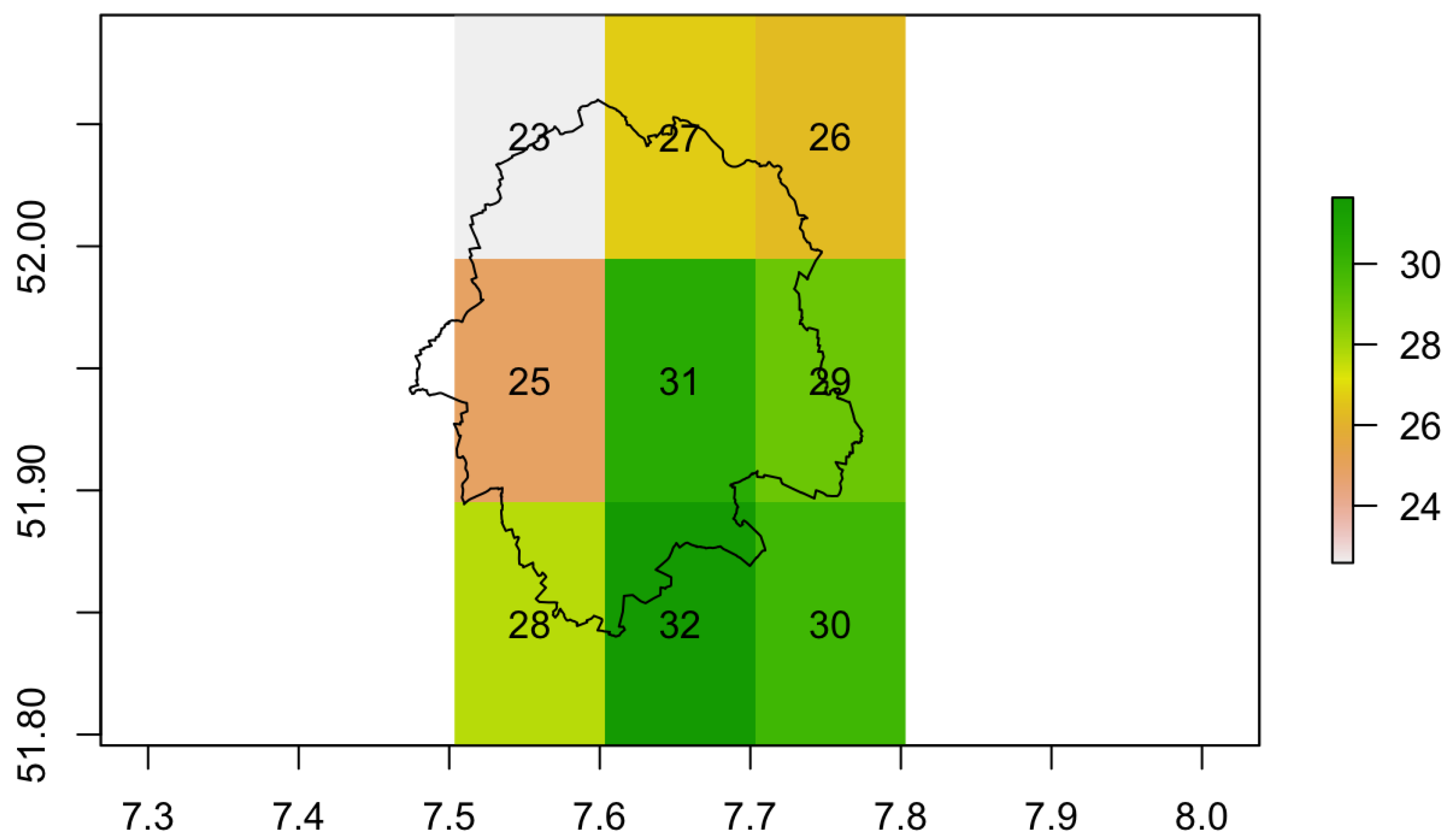
Figure 3.
Schematic overview of the proposed optimisation method. Since no LUR regression model was available for the study area at the moment of the analysis, the LUR model from the ESCAPE study was used in this paper.
Figure 3.
Schematic overview of the proposed optimisation method. Since no LUR regression model was available for the study area at the moment of the analysis, the LUR model from the ESCAPE study was used in this paper.

Figure 4.
Spatial mean prediction error achieved by SSA at different probabilities of acceptance using the optimisation method without weights.
Figure 4.
Spatial mean prediction error achieved by SSA at different probabilities of acceptance using the optimisation method without weights.
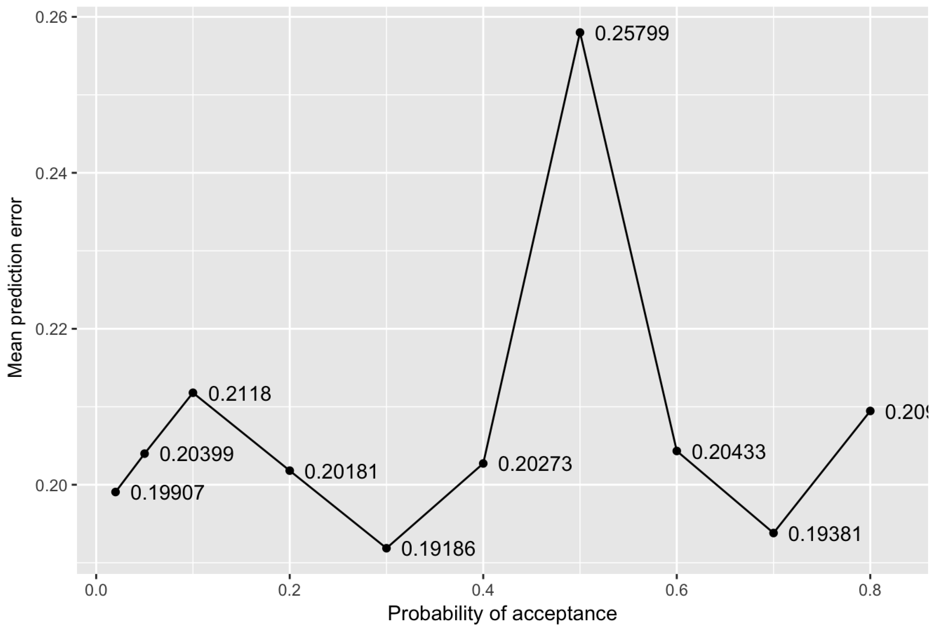
Figure 5.
Energy transition while running optimisation in SSA using parameters of 0.3 probability of acceptance after removing five higher values.
Figure 5.
Energy transition while running optimisation in SSA using parameters of 0.3 probability of acceptance after removing five higher values.
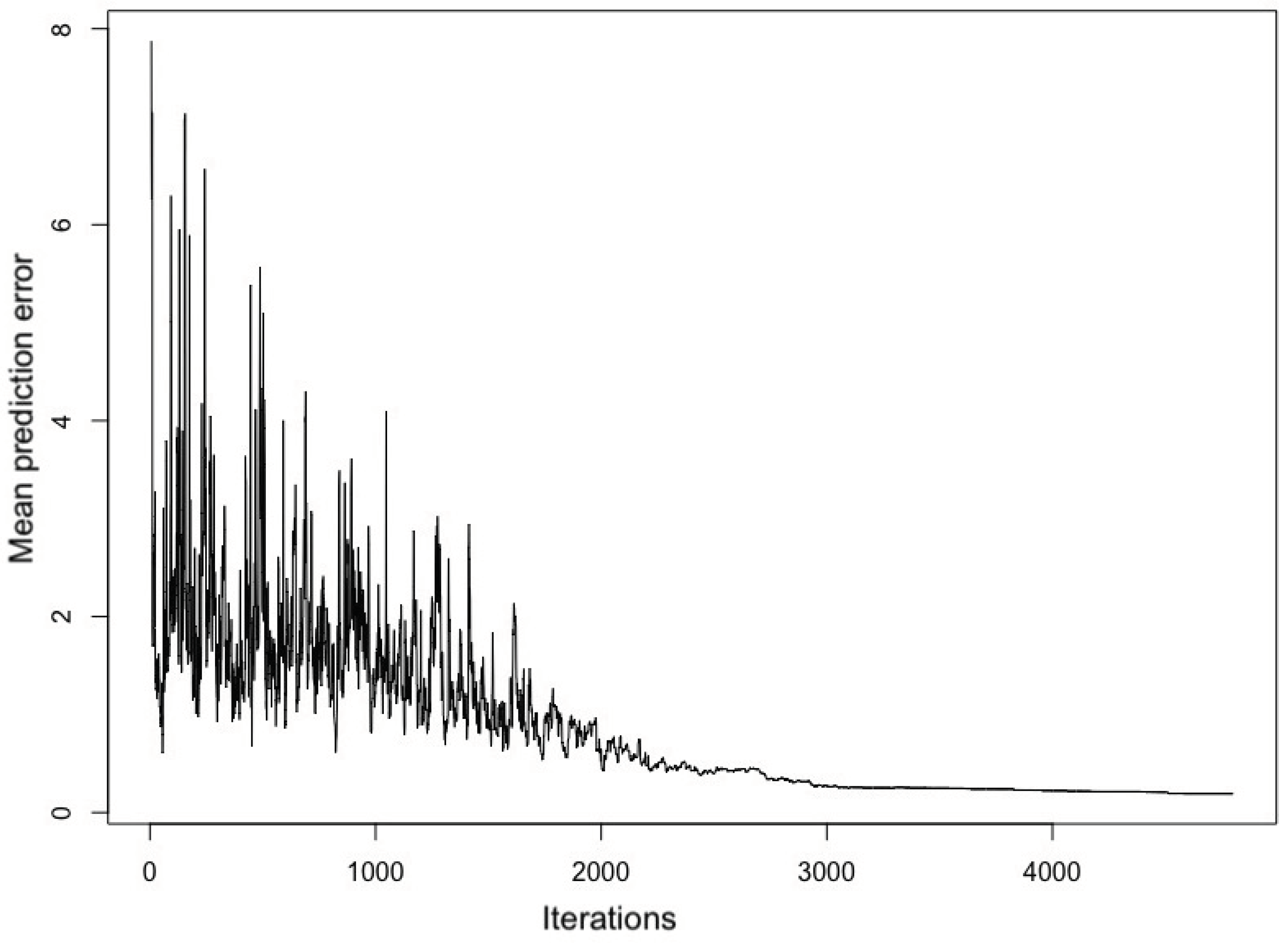
Figure 6.
Monitoring network designs realised after using the first optimisation criterion. (a) Initial monitoring network design (D0). (b) Optimised monitoring network design after using criterion.
Figure 6.
Monitoring network designs realised after using the first optimisation criterion. (a) Initial monitoring network design (D0). (b) Optimised monitoring network design after using criterion.
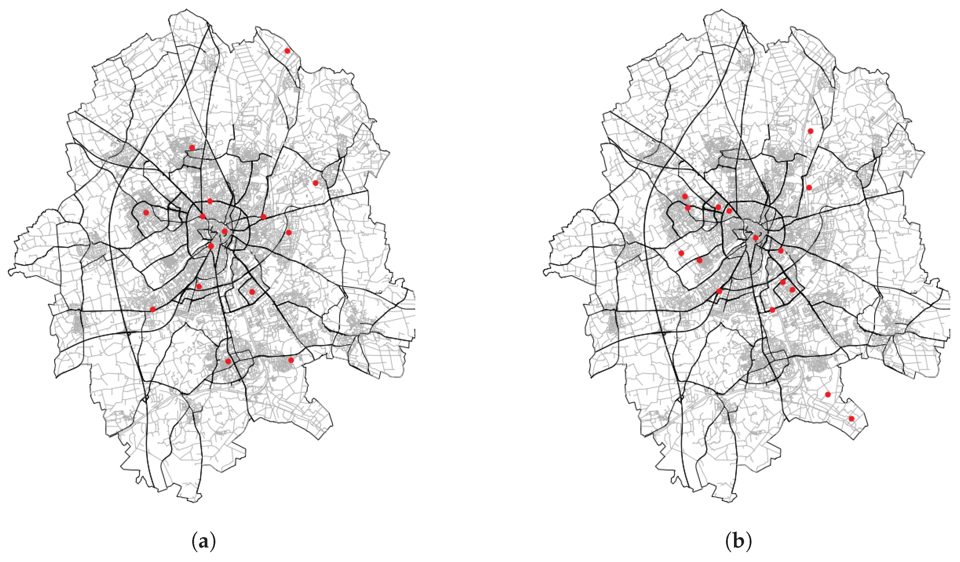
Figure 7.
Spatial mean prediction error achieved by SSA at different probability of acceptance using optimisation method with population weighted criterion.
Figure 7.
Spatial mean prediction error achieved by SSA at different probability of acceptance using optimisation method with population weighted criterion.

Figure 8.
Monitoring network designs obtained using a population weighted optimisation criterion. (a) Initial monitoring network design (D0). (b) Monitoring network design after population weighted optimisation.
Figure 8.
Monitoring network designs obtained using a population weighted optimisation criterion. (a) Initial monitoring network design (D0). (b) Monitoring network design after population weighted optimisation.
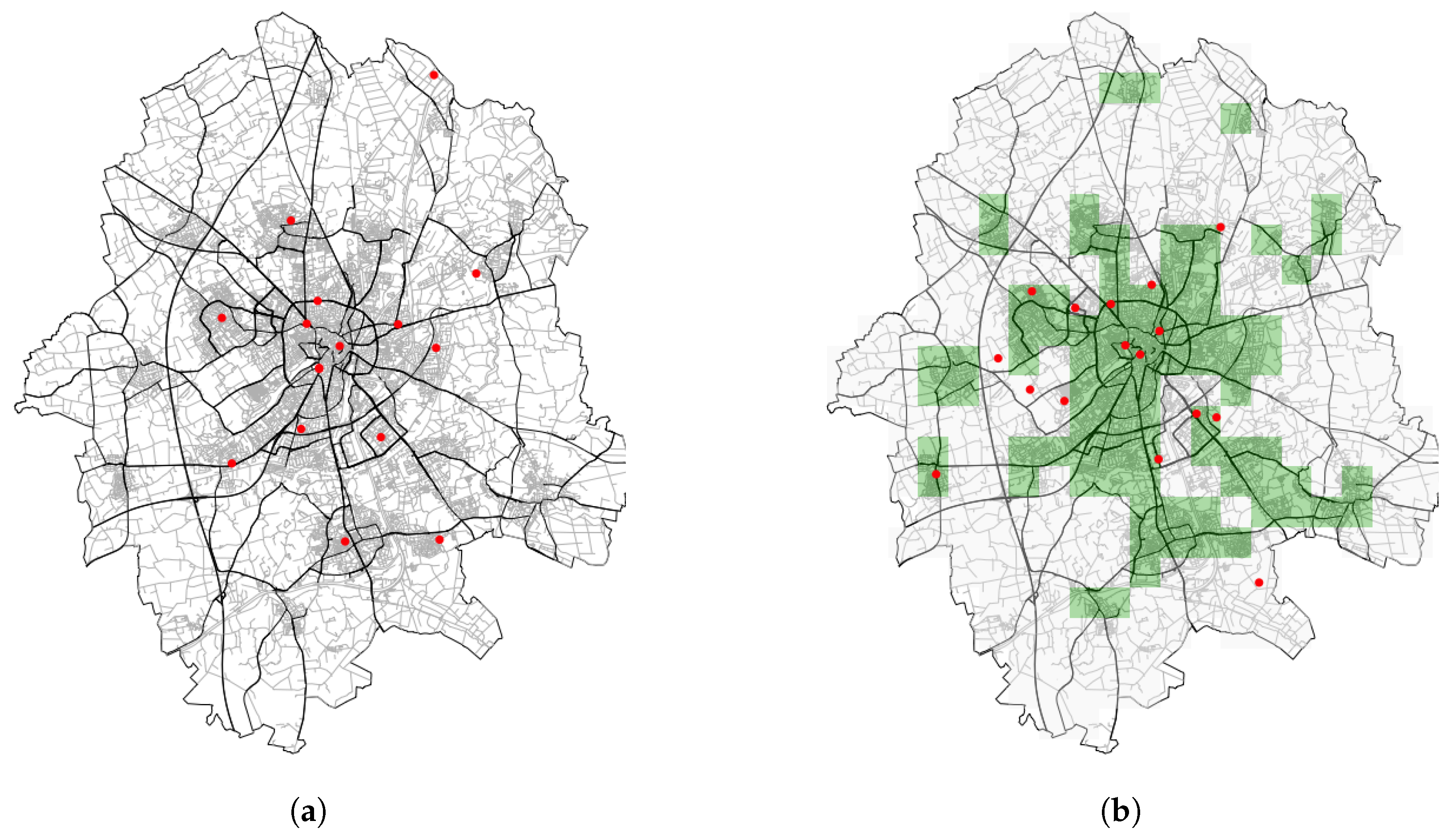
Figure 9.
Deviation of the spatial mean prediction error values from mean value obtained after 15 repetitions with same parameters.
Figure 9.
Deviation of the spatial mean prediction error values from mean value obtained after 15 repetitions with same parameters.


Figure 10.
Summary of least spatial mean prediction error values obtained for different numbers of monitoring stations .
Figure 10.
Summary of least spatial mean prediction error values obtained for different numbers of monitoring stations .
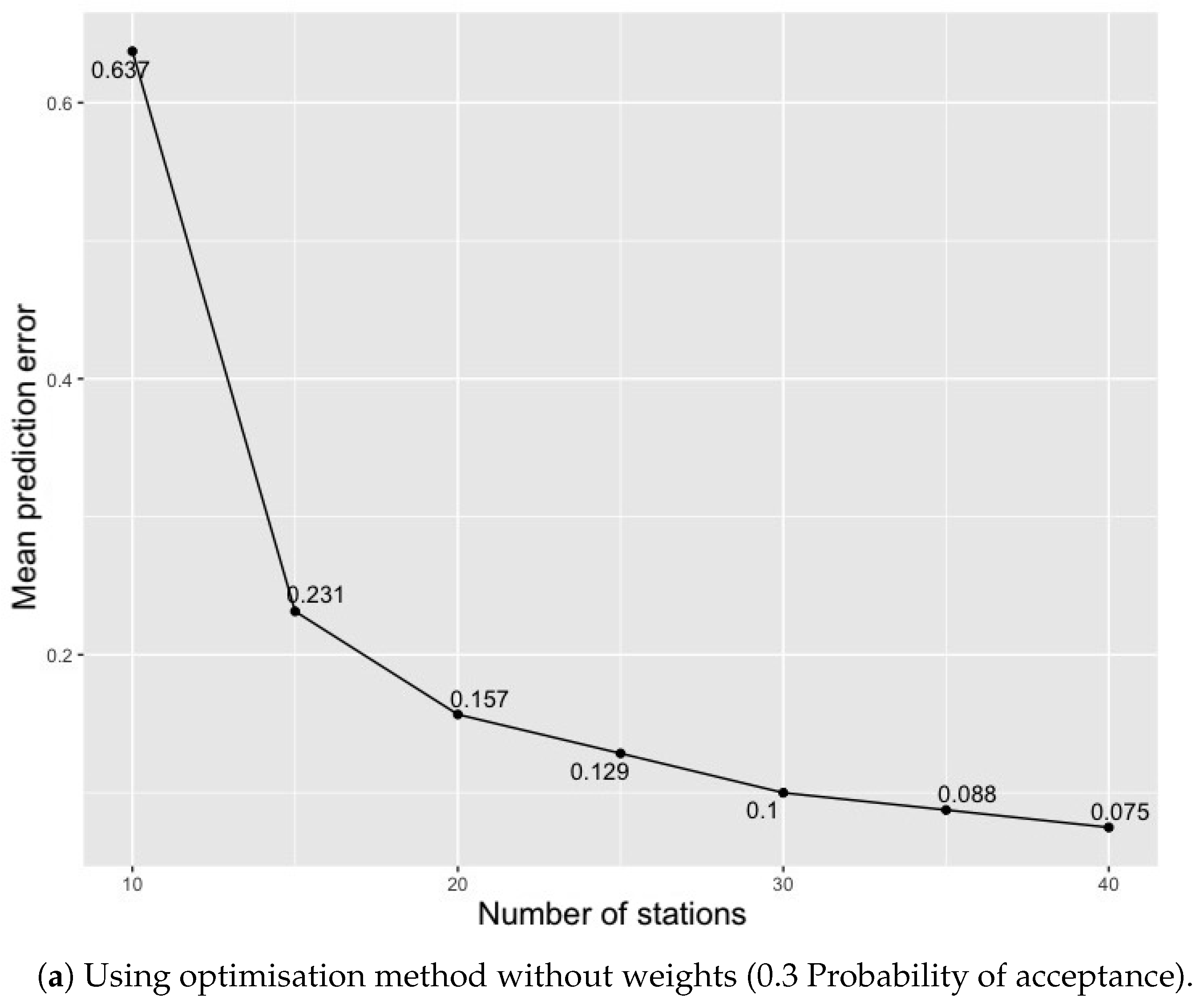

Table 1.
LUR variables selected.
| Variable | Variable Description |
|---|---|
| rdcount_1000 | Road count in 1000 m buffer |
| minrdcount_100 | Minor road count in 100 m buffer |
| minrdcount_500 | Minor road count in 500 m buffer |
| rdlength_100 | Road length count in 100 m buffer |
| rdlength_5000 | Road length count in 5000 m buffer |
| rdlength_50 | Road length count in 50 m buffer |
| mjrdlength_300 | Major road length count in 300 m buffer |
| dist.mjrd | Distance to major roads |
| minrdlength_5000 | Minor road count in 5000 m |
© 2018 by the authors. Licensee MDPI, Basel, Switzerland. This article is an open access article distributed under the terms and conditions of the Creative Commons Attribution (CC BY) license (http://creativecommons.org/licenses/by/4.0/).
Share and Cite
MDPI and ACS Style
Gupta, S.; Pebesma, E.; Mateu, J.; Degbelo, A. Air Quality Monitoring Network Design Optimisation for Robust Land Use Regression Models. Sustainability 2018, 10, 1442. https://doi.org/10.3390/su10051442
AMA Style
Gupta S, Pebesma E, Mateu J, Degbelo A. Air Quality Monitoring Network Design Optimisation for Robust Land Use Regression Models. Sustainability. 2018; 10(5):1442. https://doi.org/10.3390/su10051442
Chicago/Turabian StyleGupta, Shivam, Edzer Pebesma, Jorge Mateu, and Auriol Degbelo. 2018. "Air Quality Monitoring Network Design Optimisation for Robust Land Use Regression Models" Sustainability 10, no. 5: 1442. https://doi.org/10.3390/su10051442
Note that from the first issue of 2016, this journal uses article numbers instead of page numbers. See further details here.