Diagnosis and Treatment of the SWAT Hydrological Response Using the Budyko Framework

Abstract

The hydrologic response of a river basin pertains to how precipitation is partitioned into streamflow, evapotranspiration, and infiltration. The reliability of all these components is essential for the sustainable use of water resources. This paper seeks to understand if the prediction of the main components of the water balance from the SWAT model can be controlled and interpreted by a simple Darwinian approach: the Budyko framework. The Danube Basin was selected to assess the SWAT model green (evapotranspiration) and blue water fluxes (water yield or water that runs off the landscape into rivers) in a diagnostic approach based on two mono-parametric Budyko curve-type equations. This analysis was conducted comparing the evaporative index (EI) and the base flow index (BFI) predicted by Budyko’s equations based on observed data from 418 gauging stations with those simulated by SWAT. The study demonstrated that SWAT evapotranspiration estimations were in good agreement with those of the Budyko curves, whereas SWAT baseflow underestimated the Inn and Austrian Danube regions. The analysis of the Budyko equations in each water management region of the Danube provided a pioneering understanding of the relationship between EI and BFI in the study area, leading to an improvement of the hydrological simulations and providing a more reliable water balance in each water management region.

1. Introduction

Water resource management in river basins is an ever-increasingly challenging task mainly due to the increased demands of water and land as a consequence of global population growth, economic development, and global environmental changes. The solutions for sustainable water resource management require a better understanding of the water cycle. Hydrological modelling is largely used to understand processes that control water movement and to assess the likely impacts of future scenarios on water quantity and quality. Consequently, the quantitative understanding of hydrological components and their spatial and temporal variability in river basins is essential for an efficient planning and management of water resources [1,2].

The hydrological components have been quantified mainly using hydrological models than can be subdivided in two categories: the Newtonian and the Darwinian models. In Newtonian models, the hydrological behavior is derived from Newton’s laws, building mechanism for describing the physical processes in isolation. The Newtonian approach has numerous strengths: it is based on cause-and-effect relationships, and it is spatially explicit, having the potential to represent processes inside the catchment in major details. However, their parametrization remains a major challenge [3]. An example of a Newton model is the Soil and Water Assessment Tool (SWAT; [4]), continuous in time, semi-distributed, process-based river basin model that has been calibrated and applied in hydrological simulations throughout the world [5].

The Darwinian approaches instead aim to explain the hydrological behavior as a whole system and were developed based on empirical data from a large number of watersheds. The Budyko framework [6] is among the most known Darwinian models largely used to quantify the water balance at the watershed scale by means of a semi-empirical curve that represents the fraction of the precipitation that is lost through evapotranspiration as a non-linear function of the aridity index (ratio of potential evapotranspiration and precipitation).

In the 20th century, questions related to agriculture management pushed the continuous development and use of Newtonian models with respect to the Darwinian approaches due to the need of an explicit representation of the interactions between evapotranspiration, soil and runoff and ultimately water quality. However, on-going discussions have taken and are still taking place about model parametrization of complex Newtonian models [7]. In addition, these models are usually calibrated considering only streamflow without taking into account the partitioning of the other hydrological components, such as evapotranspiration and baseflow with the risk to have a model that was “right for the wrong reasons” since the best simulations of discharge do not coincide with the best simulations of other hydrological processes [8].

At a large scale, these models could miss the essential characteristics of what determines the real functioning of a catchment, not considering detailed hydrological processes, and not representing effectively the localized impacts [9]. The Budyko curve has been suggested as a way to constrain model parametrization [10] improving the reliability of water partitioning. In itself, the Budyko curve may also be interpreted as a criterion for model selection since a significant departure from the curve highlights a potential inconsistency of model parameterization or misrepresentation of the local dominant hydrological processes.

The main purpose of this paper is to build on an existing in-depth application of the SWAT model in the Danube River Basin [11] to examine the hydrological components of SWAT through the Budyko framework. The specific objectives are (i) to characterize the Budyko equations for the Danube Basin and across selected water management regions using observed and simulated data,(ii) to analyze the relationship between the expected Budyko curve estimations and the simulated values, (iii) to provide a general understanding of the Budyko coefficients in the study area and their control on hydrological variables, (iv) to compare the Budyko water balance with that predicted by the SWAT model, and (v) to improve the calibration of the SWAT model components in the regions that resulted inconsistent with the Budyko framework, and to present and discuss the water balance for the different water management regions.

2. Materials and Methods

2.1. The Study Area

The Danube River Basin is the second largest river basin in Europe, covering approximately 803,000 km² of Central and South-Eastern Europe. In year 2015, 19 countries were sharing the catchment, 14 of which are called “Danube countries” (with catchment areas >2000 km²). The biggest shares of the catchment belong to Romania (30%), followed by Hungary, Serbia, and Austria (around 10%) (Figure 1).

Due to its vast area and its topography ranging from lowlands to mountains above 3000 m a.s.l., the Danube River Basin exhibits a pronounced climatic variability. The western region is influenced by the Atlantic climate, whereas the eastern region is characterized by a continental climate with lower precipitation and typically colder winters. The mean annual precipitation for the whole Danube basin for the period 1980 to 2009 is 597 mm/year, ranging from 220 mm/year near the outlet of the river to 1510 mm/year in the Alps. The mean annual temperature for the period was 9.7 °C, ranging from 0.8 to 13 °C. The mean annual streamflow at the outlet was estimated around 6387 m³/s [12].

The Danube River Basin mainly consists of forest (35%), arable land (34%), and grassland (17%). The irrigated area is around 9000 km² (only ~1% of arable land), and the volume of irrigation is approximately 3 × 10⁹ m³ [13].

The main pressure types in the Danube River Basin causing hydrological alterations are impoundments, water abstractions, and hydropeaking [14]. The water abstractions for industry and public use is around 10 × 10⁹ m³ and the consumptive use for energy is 15 × 10⁹ m³ [15].

The Danube River can be divided into 18 water management regions (Figure 1;

Table 1. The 18 water management regions of Danube River Basin and their general characteristics.

ID-Regions	Name	Area (km2)	Drain Area (km2)	Mean Elevation (m) 1	Mean Annual Precipitation (mm) 2	Number of Streamflow Gauging Stations
1	Danube Source	49,769	49,769	620	950	117
2	Inn	25,999	25,999	1260	1200	75
3	Austrian Danube	26,036	101,803	800	1000	62
4	Morava	26,628	26,628	380	540	34
5	Vah-Hron-Ipel	30,587	30,587	470	720	-
6	Pannonian Danube	52,085	211,103	560	790	91
7	Drava	39,679	39,679	770	860	72
8	Sava	100,102	100,102	550	915	87
9	Tisa	149,567	149,567	360	590	75
10	Velika Morava	37,702	37,702	630	600	-
11	Middle Danube	44,261	582,414	500	790	5
12	Jiu	10,333	10,333	440	570	1
13	Olt	23,841	23,841	630	570	2
14	Arges Vedea	18,118	18,118	380	560	-
15	Silistra Danube	50,615	685,320	490	710	6
16	Buzau Ialomita	16,358	16,358	310	530	1
17	Siret-Prut	66,250	66,250	270	560	36
18	Delta	34,104	802,032	490	710	5

¹ The mean elevation was calculated from the Digital Elevation Model (DEM) CCM2 DEM [16] considering the whole drained area of each region. ² The long term mean annual precipitation in the period of simulation 1995–2009 was obtained from the ESAF-meteo database [17] considering the whole drained area of each region.

).

2.2. SWAT Model Description, Setup and Calibration

The SWAT model [4] was selected because it has a flexible structure that allows for addressing different water resource problems, it is well documented, it is an open source code that can be adapted to specific applications, and it has been used successfully throughout the world. The SWAT model is a semi-physically based, semi-distributed, basin-scale model that was applied in the Danube River Basin to simulate the water resources availability as described in Malagò et al. [11].

In SWAT, a watershed is divided into multiple subbasins, which are further subdivided into hydrologic response units (HRUs) that consist of a unique combination of soil, land use/cover, and slope. The overall hydrologic balance is simulated at daily time step for each HRU, summarized at the subbasin level, and then routed through the stream network to the watershed outlet.

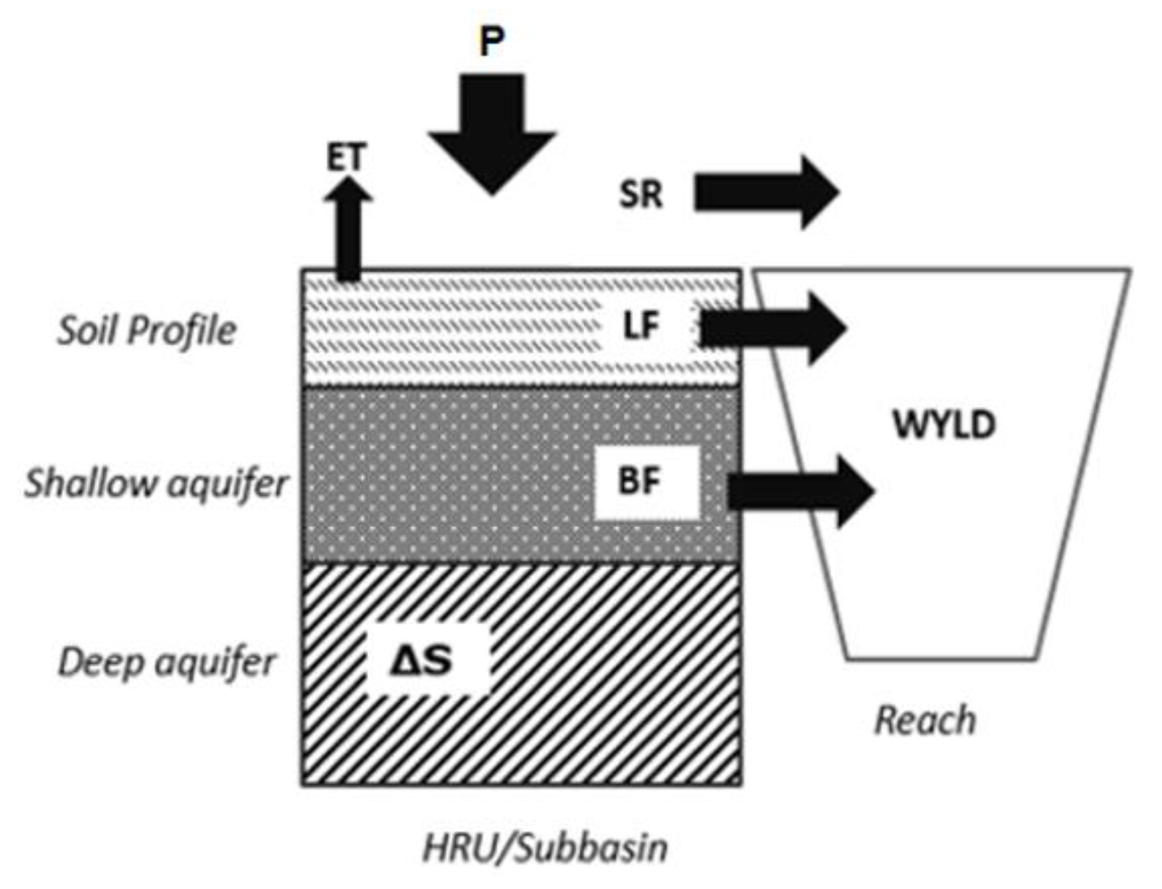
The water balance, illustrated in Figure 2, can be expressed as follows:

$$\mathrm{P}=\mathrm{ET}+\mathrm{SR}+\mathrm{LF}+\mathrm{BF}+\Delta \mathrm{S}$$

(1)

where P is the precipitation (mm), ET is the evapotranspiration (mm), SR is the surface runoff (mm), LF is the lateral flow contribution to stream flow (mm), BF is the baseflow contribution to streamflow from the shallow aquifer, and ΔS is the water storage in the shallow and deep aquifers.

The potential evapotranspiration (PET) was estimated using the Penman-Monteith method [18] and the actual evapotranspiration (ET) was calculated including the processes of canopy interception, crop transpiration and soil evaporation as described in Neitsch et al. [19]. The surface runoff (SR, mm) was estimated using the SCS curve number method [20] as modified by Williams [21] to account for the impact of slope on the curve number. SWAT uses two linear reservoirs to partition groundwater into two aquifer systems: a shallow aquifer that contributes baseflow to streams (BF), and a deep aquifer that can also contribute baseflow to streams. The remaining portion in the deep aquifer can be considered lost from the system. In this work the contribution of baseflow from deep aquifer was considered negligible and was thus set to zero. The recharge of the aquifer for a specific day is calculated as a linear function of the daily seepage, the recharge of the previous day, and the groundwater delay. The lateral flow (LF, mm) occurs whenever the soil water content exceeds field capacity and is calculated as a function of the drainable volume of water stored in the saturated zone of the HRU per unit area (mm), the saturated hydraulic conductivity (mm/h), the drainable porosity of the soil (mm/mm) and the hillslope length (m). The baseflow (BF) from the shallow aquifer is calculated based on the aquifer recharge parameter, the deep aquifer recharge and the baseflow recession constant. The total blue water fluxes leaving the HRU and entering into the main channel during the time step is termed water yield (WYLD) and is estimated as the sum of SR, LF, and BF.

The SWAT model requires five basic input data sets: topography, soil, land use, climatic data and management data. The Danube watershed was subdivided in 4663 subbasins based on the Digital Elevation Model CCM2 DEM [16] with 100 m pixel size. The climate data, including daily precipitation, temperature, solar radiation, wind speed and relative humidity, were obtained from EFAS-METEO at spatial resolution of 5 km × 5 km [17] for the period 1990–2009. To account for the increase in precipitation with elevation that is typically observed in mountainous regions, four elevation bands were implemented. The landuse was defined using a map of 1 × 1 km for year 2000, built from the combination of CAPRI [22], SAGE [23], HYDE 3 [24], and GLC databases [25]. The crops were distributed on dominant arable land subbasins according to European statistics at NUTS2 level (administrative subdivision) [26]. The soil map of 1 × 1 km was obtained from the Harmonized World Soil Database (HWSD) [27]. Based on the combination of land use, soils, and slope, the Danube Basin was discretized into 5181 HRUs with a median area of 129 km².

The simulation period was 1990–2009 including five years used as warm-up to mitigate the unknown initial conditions. In short, a regionalized calibration and validation procedure was developed and applied to ensure that monthly streamflow and its components were correctly simulated. The hydrologic parameters were calibrated in 264 headwaters for the period 1995–2006, followed by a regionalization of the calibrated parameters. The model was then validated in 708 stations for the period 1995–2009. After calibration and regionalization, about 70% of the gauging stations of the calibration dataset reached satisfactory percent bias (PBIAS ≤ ±25%) comparing the observed and simulated monthly streamflow. From the validated dataset, 60% of the gauging stations reached satisfactory performance. Additional details about the SWAT and calibration can be found in Malago’ et al. [11].

2.3. The Budyko Framework

Considering the long term mean annual water balance at watershed scale, assuming that the water storage change (ΔS) is negligible, the mean annual precipitation (P) can be partitioned into surface runoff SR, identified as the total streamflow (Q), and evapotranspiration (ET) as follows:

$$\mathrm{P}=\mathrm{ET}+\mathrm{Q}$$

(2)

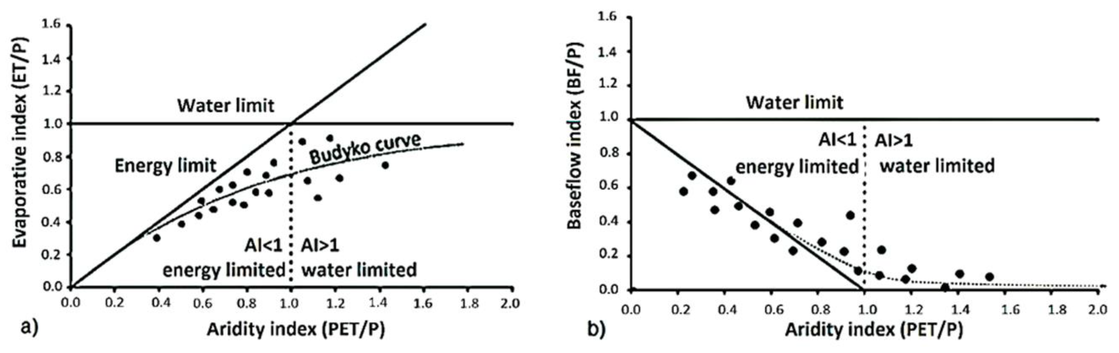
Budyko [28] postulated that the partitioning of precipitation could be determined by the competition between available water (in terms of precipitation) and the available energy approximated by the potential evapotranspiration (PET). Such water and energy coupling is represented in a bi-dimensional space relating two dimensionless variables: the evaporative index (EI) calculated as the ratio of evapotranspiration (ET) and precipitation (P) and the aridity index (AI) calculated as the ratio of PET and P (Figure 3a). The Budyko approach is then expressed as

$$\frac{\mathrm{ET}}{\mathrm{P}}=\mathrm{f}\left(\frac{\mathrm{PET}}{\mathrm{P}}\right)$$

(3)

The evaporative index (ET/P) can be considered a measure of the long-term mean annual water balance in a watershed, since it is the fraction of the water falling as precipitation that is lost as evapotranspiration. On the other hand, the aridity index (PET/P) is a measure of the long-term mean annual climate being a ratio between the energy availability (PET) and the water availability (P). Budyko [6,28] carried out an empirical analysis of the long term mean annual balances in a large number of watersheds around the world and demonstrated that the water balance of equation 2 in different climatic regions provided a nice fit to the curve (called the Budyko curve, Figure 3a). The curve has two physico-mathematical limits: (i) under very dry conditions (AI > 1, water limit) ET will approach P, i.e., in arid regions the available energy greatly exceeds the amount required to evaporate the entire annual precipitation; (ii) under very wet conditions (AI < 1, energy limit) ET will asymptotically approach the unity that means that in humid regions the available energy (PET) is only a fraction of the total annual P.

In this study a mono-parametric Budyko-type equation developed by Yang et al. [29] was used. The equation can be written as

$$\frac{\mathrm{ET}}{\mathrm{P}}={\left[1+{\left(\frac{\mathrm{PET}}{\mathrm{P}}\right)}^{-n}\right]}^{-\frac{1}{n}}$$

(4)

where n is the parameter that captures the combined effects of river basins and vegetation characteristics.

Recently, Wang and Wu [31] defined a complementary Budyko-type equation for the estimation of the baseflow index (BFI = BF/P) assuming that at annual scale in steady-state conditions the baseflow (BF) is mainly controlled by the aridity index, and the surface runoff components is hypothesized as negligible. A complementary mono-parametric Budyko-type equation was formulated as follows:

$$\frac{BF}{P}=1-{\left[1+{\left(\frac{PET}{P}\right)}^{-m}\right]}^{-\frac{1}{m}}$$

(5)

where m is the complementary n parameter of Equation (4) that represents the effects of other factors that can influence the baseflow generation (i.e., elevation, snow melt and slope). This equation has a limit represented by the line 1:1 shown in Figure 3b. Under very wet conditions (AI < 1), the data points of BF/P must not to exceed this line, i.e., BF/P < 1 − PET/P, and we expect that they asymptotically approach the limit when AI is near 0.

The Budyko n and m parameters of Equations (4) and (5) were calibrated on the Danube River Basin based on data of ET, BF and PET from 418 gauged stations well distributed across the basin (Figure 1). The best n and m parameters were identified using a simple non-linear least squares curve fitting function. The long term mean annual PET and P were retrieved from the SWAT model simulations in the period 1995–2009.

EI from observation (EI_obs) was calculated as the difference between the long term mean annual precipitation (P) and the observed mean annual streamflow (Q) during the period 1995–2009 divided by precipitation. The observed BF (BF_obs) was extracted from measured daily streamflow time series at the 418 gauging stations, and then aggregated at annual time step. A digital filter [32] was used to perform the separation of the components of the streamflow. Finally, BFI was calculated dividing BF_obs by the mean annual precipitation.

2.4. The Diagnostic Analysis of SWAT Hydrological Fluxes

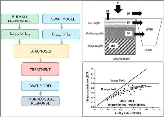
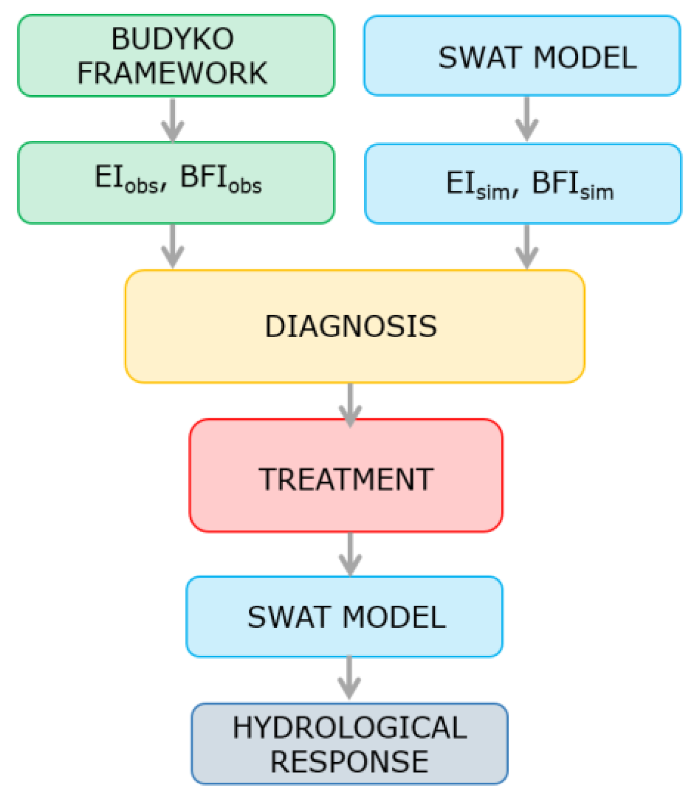
The two mono-parametric Budyko-type Equations (4) and (5) were used to explore the reliability of the main components of the water balance, the evapotranspiration and baseflow, as simulated by the SWAT model. A diagnosis-treatment approach was used following the key medical principles [33] using the following sequential schema (Figure 4):

• examination of the hydrological components through the application of a Newtonian model (the SWAT model) and a Darwinian model (the Budyko approach);
• diagnosis to screen the potential causes of the inconsistencies of SWAT with the Budyko hypothesis;
• application of a treatment constraining the parameters that wrongly affect the process.

In particular, we examined the hydrological components derived from the SWAT model and the Budyko framework. The derived observed Budyko curves were used as a reference to perform a diagnosis of the SWAT predicted components. Thus, the scatter points of the SWAT evaporative index against the corresponding aridity index in each subbasin of the modeled area were plotted in the Budyko diagram. Each point that represents a subbasin in the study area was analyzed considering the catchment physical characteristics such as elevation, slope, precipitation and percentage of area covered by crop land. A specific analysis of EI and BFI of the 18 main water management regions in the Danube Basin (Figure 1) were also performed. The diagnosis analysis was pursued focusing on the Budyko curves derived from SWAT components to investigate the simulated n and m coefficients in each water management region.

After the accurate diagnosis, a screening of the potential causes of the inconsistencies of SWAT predictions with the Budyko hypothesis were investigated and a treatment was applied. The treatment consisted in constraining the parameters that affect the processes wrongly simulated.

3. Results and Discussion

3.1. The Calibrated Budyko Theoretical Equations

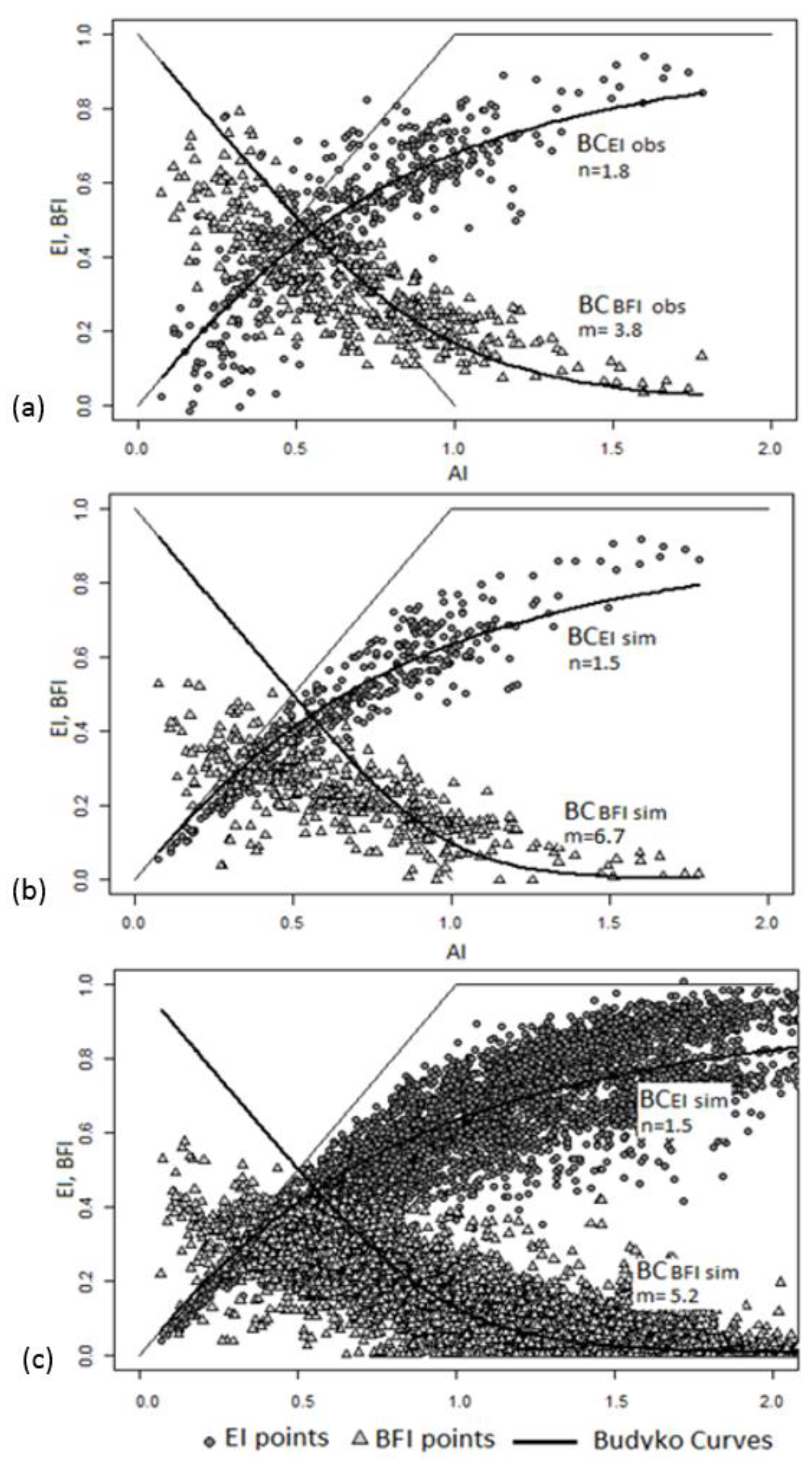
Figure 5 shows the Budyko curves based on the observed values at the 418 selected gauging stations in terms of EI, BFI and AI. The best fitted values of n and m were 1.8 and 3.8, respectively, and hereafter were used as reference values. Figure 5a shows that some subbasins are located outside the energy limit highlighting that for these subbasins there is an external source of water (i.e., karst area, etc.).

Similarly, Figure 5b shows the Budyko curves calibrated using the simulated values by SWAT at the 418 gauged selected subbasins. The coefficient n was estimated equal to 1.5, very similar to that of the Budyko curve of the observations. Instead, the coefficient m was estimated equal to 6.7, about twice the m obtained using the observed values. It is noteworthy that the subbasins in terms of EI and AI are located below the energy limit, highlighting that the model had properly apportioned precipitation among ET, surface runoff and infiltration as no external water was introduced in the SWAT setup. In terms of BFI and AI the subbasins characterized by AI < 0.5 diverged significantly from the limit of Budyko curve for the BFI.

Similar findings were observed when using the SWAT results for all subbasins of the Danube (Figure 5c). The coefficient n was the same of the Budyko curve of the gauged subbasins and m resulted equal to 5.2.

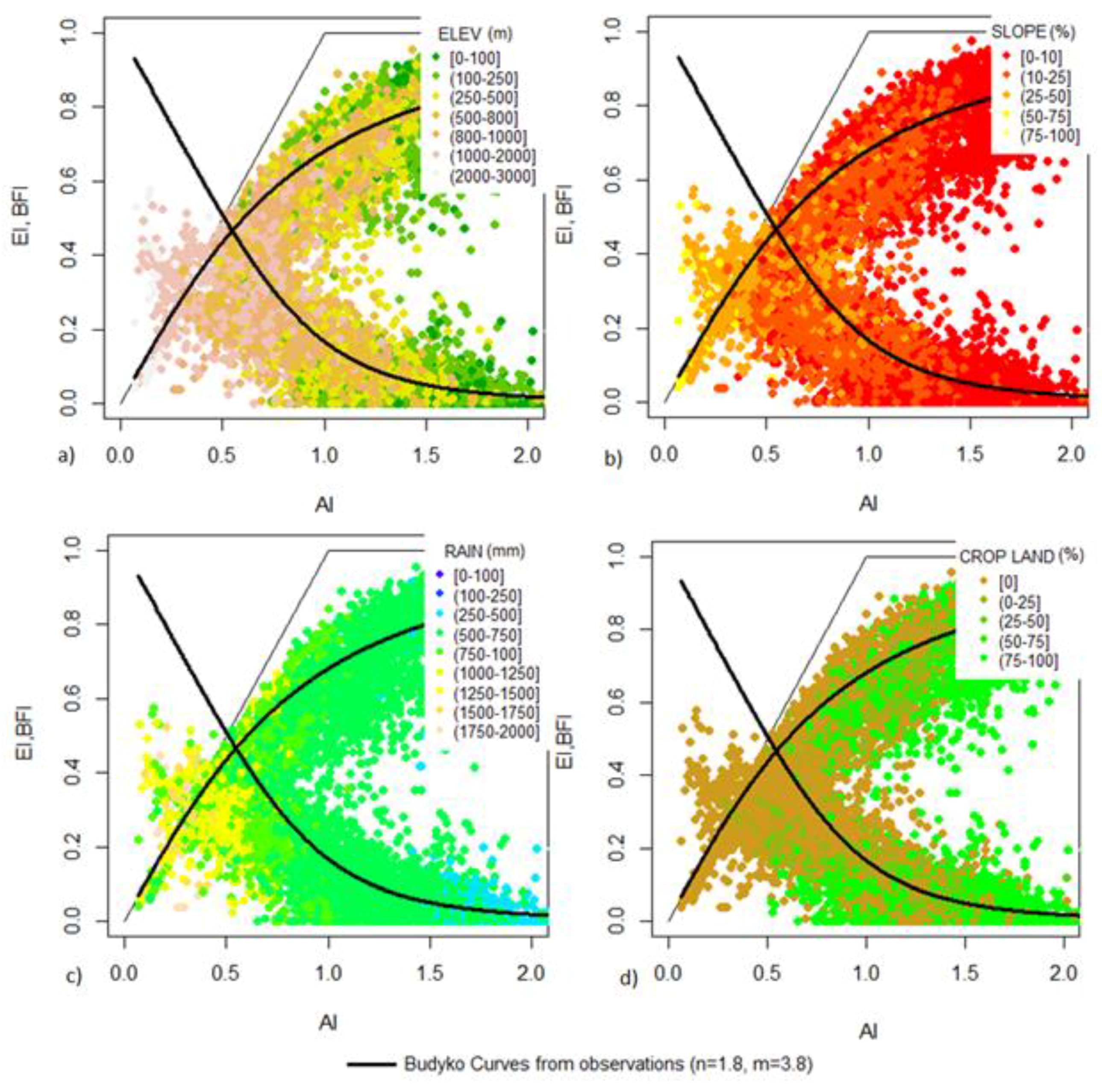
Figure 6 depicts the relationship between AI-EI, and the complementary relationship BFI-AI, considering all subbasins in the Danube, as affected by elevation, slope, precipitation and percentage of area covered by crop land. The simulated EI was lower in the subbasins characterized by lower AI, such as in subbasins with high elevation, steep slope, and abundant precipitation, since the temperature is generally too low for generating higher EI. Conversely, EI is higher in flat crop land subbasins with low precipitation.

Concerning the BFI, it is noticeable that the index resulted underestimated in wet or humid subbasins (AI < 0.5) characterized by high elevation, steep slope, rich precipitation, and mainly covered by forest and pasture as shown in Figure 6d by the brown points (subbasins with higher percentage of forest and pasture compared to crop land).

3.2. The n and m Budyko’s Coefficients for Water Management Regions

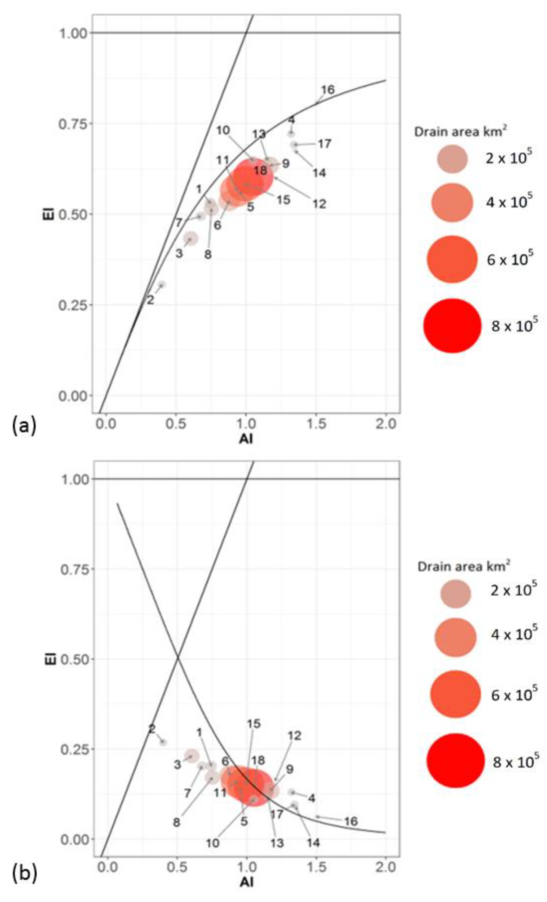
The Budyko-type curves were also calculated in each water management region, calibrating for each of them the coefficients n and m using the simulated values of SWAT. Figure 7a,b show the spatial distribution of these coefficients, while Figure 8a,b show the relationship between the Budyko coefficients in the 18 water management regions with respect to the coefficients n = 1.8 and m = 3.8 obtained using the observations.

Comparing n and m among the regions (Figure 7), it can be observed that generally in the all water management regions the n coefficient was in the range of 1.4–1.6, except for regions 2 (Inn), 12 (Jiu) and 14 (Olt) and for region 16 (Buzau-Ialomita), 17 (Prut-Siret) and 7 (Drava). The coefficient m was around 3 in the region 4 (Morava) and 12 (Jiu), in the range 4–6 in all the other regions except in region 1 (Upper Danube), 2 (Inn), 3 (Austrian Danube), 7 (Drava), and 8 (Sava). In particular, the highest value of m was found in the region 2 (Inn River Basin). In particular, the Inn Basin (region 2) differed from the comprehensive Danube behavior, with the lowest n (equal to 1.3) and the highest m (more than 20), the Drava Basin (basin 7) had instead the highest n (equal to 2) and high m coefficient (equal to 18), whereas the Sava (region 8) had n equal to 1.5 and a significantly higher m equal to 16.5.

Concerning the AI-EI relationship (Figure 8a), all the regions are well distributed near the Budyko curve and, as expected, the Inn Basin (region 2) and Austrian Danube (region 3) had the lowest EI values since they are humid regions characterized by AI < 1. Conversely, for instance, the Morava River Basin (region 4) and the Buzau-Ialomita (Region 16) had higher values of EI since they are classified as arid basins with AI > 1. The differences in percentage between the theoretical EI of the Budyko curve and those simulated by SWAT were below 20%. The regions 16 (Buzau Ialomita), 4 (Morava), and 1 (Danube Source) had the lowest differences and for the whole Danube the difference was around 13%. The AI-BFI relationship (Figure 8b) shows that the Inn basin (region 2) and the Austrian Danube (region 3) are located correctly below the Budyko curve but too low with respect to the limit, thus indicating a likely underestimation of BFI.

Considering these results, Figure 9 provides a general understanding of the n-m relationship with respect to the EI and BFI as simulated by SWAT in each region. Decreasing the n coefficient and increasing the m coefficient the baseflow index becomes significant and the evaporative index negligible. This is the case of the Inn basin (region 2). Conversely, increasing n and decreasing m, the baseflow is negligible and the evaporative index becomes an important factor in the water balance. This is the case of Siret-Prut (basin 17) and Ialomita (basin 16). Increasing both n and m, both the evaporative and baseflow index are important (i.e., in the Drava basin, basin 7). As a consequence, this analysis shows that not only the n coefficient has a key role in the hydrological responses but also the coefficient m and in particular in humid areas.

3.3. The Reliability of the SWAT Model Hydrological Simulation

The previous results highlighted that the model suffers for an underestimation of BFI in the regions characterized by AI < 0.5. The differences in percentage between the theoretical BFI of the Budyko curve and those simulated by SWAT were markedly evident across the Danube (Figure 10), in particular in the Inn River Basin (Region 2).

This underestimation has influenced also the predicted streamflow that was characterized by a bias of 27% with respect to the observed streamflow (

Table 2. Comparison between the mean annual observed streamflow at the outlet (or near the outlet) and the SWAT simulated values before and after the treatment. In evidence the main changes in the Inn, Austrian Danube, and at the Delta. ΔQ is the difference in percentage between observed and predicted mean annual streamflow.

ID-Regions	Name	Gauged Station	Mean Annual Observed 1 Streamflow at the Outlet (m3/s) Period 1995–2009	Mean Annual Simulated before the Treatment Streamflow at the Outlet (m3/s) Period 1995–2009	Mean Annual Simulated after the Treatment Streamflow at the Outlet (m3/s) Period 1995–2009	ΔQ before Treatment	ΔQ after Treatment
1	Danube Source	Hofkirchen (47,690 km2)	651	590	590	9%	9%
2	Inn	Passau Ingling (outlet)	759	555	626	27%	18%
3	Austrian Danube	Wien-Nussdorf (outlet)	1969	1594	1665	19%	15%
4	Morava	Zahorska Ves (outlet)	109	146	146	−34%	−34%
5	Vah-Hron-Ipel	Komarno on Vah Basin (outlet); Kamenin on Hron (outlet); Salka on Ipel (outlet)	245	259	259	−6%	−6%
6	Pannonian Danube	Hercegszanto (208,600 km2)	2350	2217	2288	6%	3%
7	Drava	Dravaszabolcs (37,480 km2)	505	504	504	0%	0%
8	Sava	Sremska Mitrovica (91,920 km2)	1402	1322	1322	6%	6%
9	Tisa	Szeged (138,600 km2)	914	984	984	−8%	−8%
10	Velika Morava	NA2	NA	258	258	NA	NA
11	Middle Danube	Pristol/Novo (outlet)	5457	5590	5660	−2%	−4%
12	Jiu	Podari (9728 km2)	88	77	77	13%	13%
13	Olt	Cornet (13,950 km2)	113	109	109	4%	4%
14	Arges Vedea	NA	NA	117	117	NA	NA
15	Silistra Danube	Chiciu/Silitra (outlet)	6221	6100	6172	2%	1%
16	Buzau Ialomita	Cosereni on Ialomita (6337 km2)	37.98	35	35	8%	8%
17	Siret-Prut	Lungoci on Siret (36,220 km2); Confluence Danube at Giurgiulesti on Prut Basin (28,420 km2)	323	322	322	0%	0%
18	Delta	Delta (outlet)	6680	6508	6580	3%	1%

¹ Details about the sources of observed values can be found in Malago’ et al. [11]. ² NA = not available information.

).

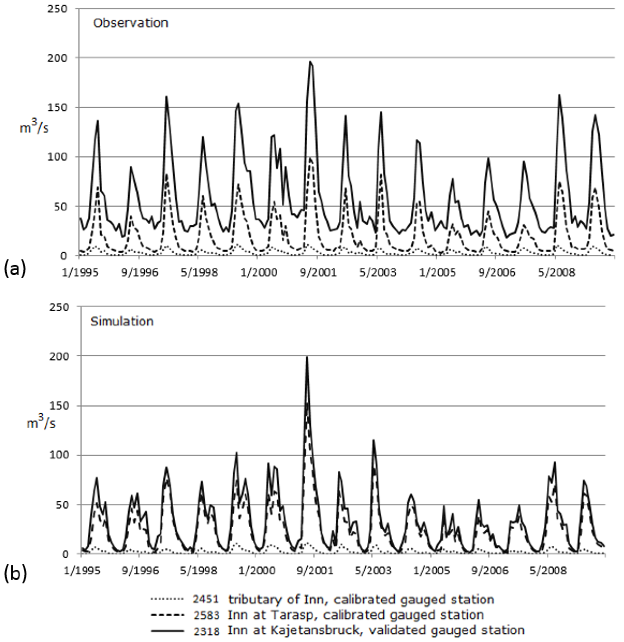
The simulated (SWAT) water balance (

Table 3. Mean annual water balance for each water management region in the Danube Basin as simulated with SWAT for the period 1995–2009 before and after the treatment. P: precipitation (mm); ET: evapotranspiration (%); SR: surface runoff (%); LF: lateral flow (%); BF: baseflow; ΔS = storage in aquifer (%); WYLD: water yields (%). The balance refers to each region considering the upstream area. In evidence the changed percentages for the Inn Basin.

Region	Name	Before Treatment						After Treatment
		ET	SR	LF	BF	ΔS	WYLD	ET	SR	LF	BF	ΔS	WYLD
1	Danube Source	53	19	1	20	7	40	53	19	1	20	7	40
2	Inn	31	21	7	27	14	55	31	21	7	34	7	62
3	Austrian Danube	43	21	3	23	10	47	43	21	3	25	7	49
4	Morava	72	13	0	13	1	27	73	14	0	13	0	27
5	Vah-Hron-Ipel	58	20	1	13	8	34	58	20	1	14	7	34
6	Pannonian Danube	54	19	2	18	7	39	54	19	2	19	6	40
7	Drava	49	19	3	20	8	42	49	19	3	20	8	42
8	Sava	51	25	1	17	5	43	52	25	1	17	5	43
9	Tisa	63	20	0	13	3	34	64	20	0	14	2	34
10	Velika-Morava	65	18	2	11	4	31	65	18	2	11	4	31
11	Middle Danube	57	20	1	16	6	38	57	20	1	17	5	38
12	Jiu	60	19	1	16	4	36	61	19	1	16	3	36
13	Olt	65	21	1	12	2	33	65	21	1	12	2	33
14	Arges-Vedea	67	22	0	8	2	31	68	22	0	8	1	31
15	Silistra Danube	58	20	1	15	5	37	58	20	1	16	4	37
16	Buzau-Ialomita	78	13	0	6	2	20	80	13	0	7	0	20
17	Siret-Prut	73	16	1	9	1	26	73	17	1	10	0	27
18	Delta	60	20	1	14	5	35	61	20	1	15	4	36

) of the Inn River Basins showed that 31% of the precipitation is lost by evapotranspiration, 55% contributes to water yield (21% surface runoff, 7% lateral flow and 27% baseflow) and 14% of precipitation is lost to deep aquifer recharge. This means that there is a considerable amount of water lost by the system that could contribute to baseflow. These findings immediately suggested that the calibrated headwaters used as donors in the regionalization were strongly influenced by derivations, storage of water outside the subbasins, as well as water released in other subbasins. It is noteworthy that the Inn River and its alpine headwaters are strongly influenced by anthropogenic activities. Water resources are intensively used by agriculture, tourism, industry and energy providers [34]. Furthermore, the Inn River Basin is ideally suited for hydroelectric power generation due to its high precipitation and runoff rates. The biggest runoff-river power plants are installed along the main river, and the most important reservoir power plants with a range of 50–1000 GWh are situated in the southern part in the Central Alps [35]. As a consequence, the calibrated parameter sets transposed in the hydrological similar subbasins led to misrepresent the behavior of the Inn Basin as shown in Figure 11 and Figure 12. The gauging stations in the subbasins 2583 and 2451 were independently calibrated and used as donors in the regionalization since human impacts were initially assumed negligible.

Rossi [36] reported that from Inn at S-Chanf, Vallember, Varush, and Tantermozza (Figure 11), the water is stored and diverted to the Ova Spin hydroelectric plant through a pressure pipe. The Ova Spin collects the important contribution from the compensating basin of Spol (33 m³/s) and continues in a pressure pipe parallel to Inn, collecting other water until the Pradella hydroelectric power plant, situated on the Inn, with an average discharge of 66 m³/s (Figure 11). From this point, another water diversion in a pressure pipe runs for 14 km until the Martina hydroelectric plant on the Inn River, with a discharge of 88 m³/s. After that, the Inn River receives a negligible contribution from subbasin 2451 and at the gauged station Kajetansburk (2318) the streamflow resulted strongly influenced by the Martina plant.

Figure 12a shows the monthly observed streamflow on Inn at Tarasp (subbasin 2583), after the diversion and before the Pradella hydroelectric plant, and at Kajetsnsbruck (subbasin 2318) after the Martina plant. The figure shows the negligible contribution of basin 2451 highlighting the strong impact of Martina plant on Kajetsnsbruck gauged station (subbasin 2318).

In SWAT, the calibrated parameters of subbasin 2583 were transposed to the hydrologically similar uncalibrated subbasin 2318. The simulated streamflow in subbasin 2318 (Figure 12, Kajetsnsbruck station) resulted underestimated since the anthropogenic contribution from Martina plant and the diversion upstream were not initially considered in the modelling.

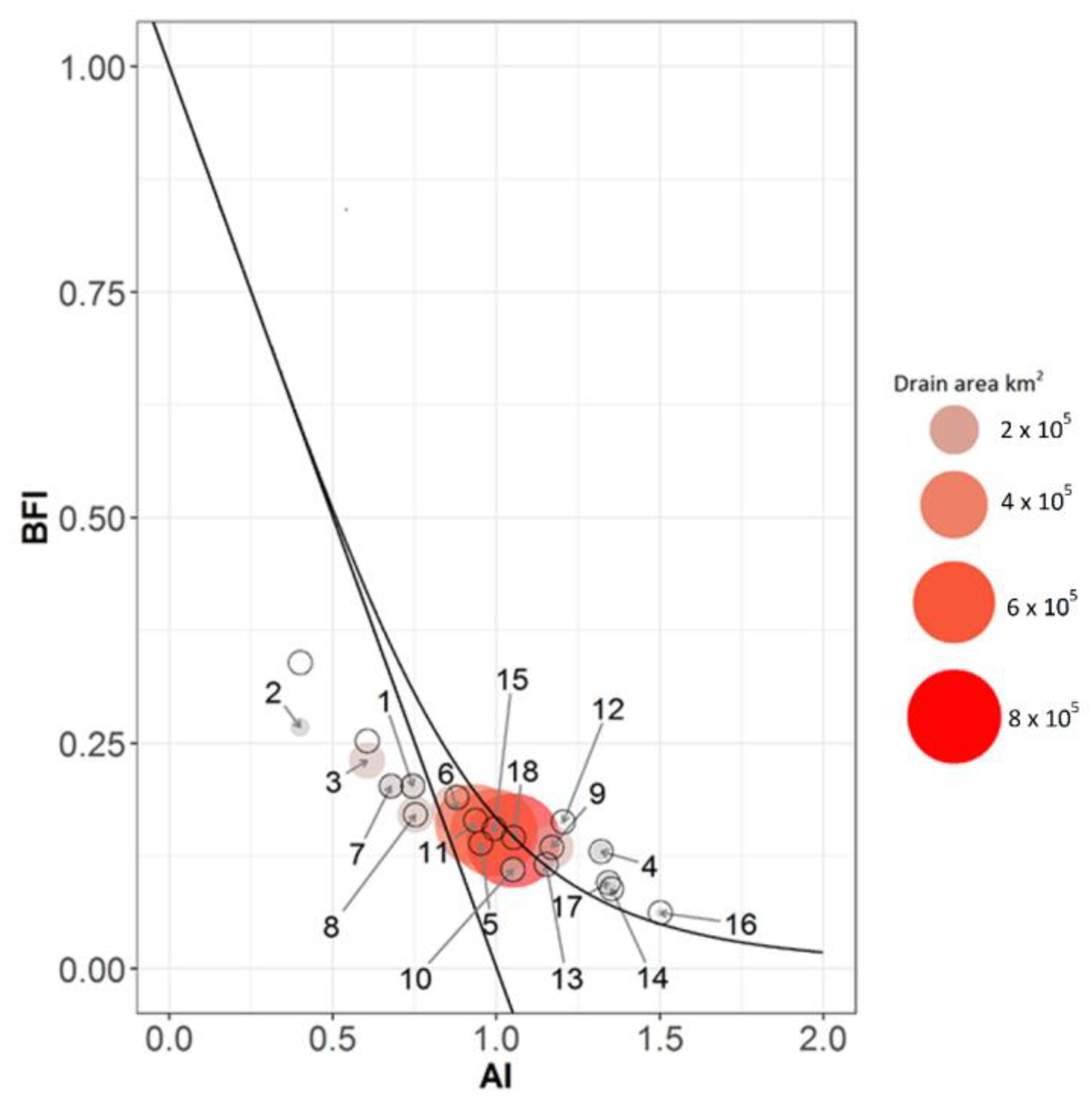
We then manually improved the parametrization in this water management region, and Figure 13 shows the relationship between EI and BFI before and after the manual modification of the deep aquifer recharge coefficients. It is noticeable that the water lost from the system as deep aquifer recharge improved the BFI estimation, moving the points closer to the Budyko curve.

Concerning the other regions, it is noteworthy that larger differences in percentage between the theoretical BFI and that simulated by SWAT were also observed in region 4 (Morava), region 12 (Jiu) and 17 (Siret-Prut). However, the BFI in these regions could be considered acceptable since the regions in terms of relative actual evapotranspiration and aridity index well approximated the theoretical Budyko curves.

The improvement of the parametrization of deep aquifer recharge in the Inn River Basin has allowed obtaining better model performance as reported in Table 2. The difference in percentage between observed and simulated mean annual streamflow for the period 1995–2009 decreased from 27% to 18% for the Inn River Basin, from 19% to 15% in the Austrian Danube and from 3% to 1% at the Delta.

The Water Balance of the Danube River Basin

The Darwinian approach has helped to identify the subbasins with potential errors in evapotranspiration and baseflow estimation. Based on the previous insightful findings, the calibration in the Inn River Basin was manually adjusted, improving the reliability of baseflow estimation. The water balance components in percentage before and after the treatment are reported in Table 3. In particular, the baseflow index increased from 27% to 34% while decreasing the deep aquifer recharge from 14% to 7% of precipitation.

The results reported in Table 3 can be compared with numerous studies that applied hydrological models in the Danube River Basins. Fehér and Muerth [37] provided an exhaustive water models inventory for the Danube Region giving details of models’ structure, spatial and temporal scale, as well as their project studies, main references and the aims of the application. Among these studies, the SWAT model results were compared with the mean values reported by Petrovič et al. [38] and EnviroGRIDS [39]. Petrovič et al. [38] used WatBal model [40] in the Danube regions for the period 1961–1990, while EnviroGRIDS [39] used SWAT to simulate streamflow and nutrients in the whole Black Sea Basin [41].

For the Danube River Basin it was estimated that 60% of the precipitation is lost through evapotranspiration (ET), 35% is water yield and only a 5% is storage in the aquifers. This water balance is similar in the Silistra Danube (Region 15) and in the Middle Danube (Region 11). Both of the aforementioned studies show very close percentages of evapotranspiration and water yield to the one estimated in this study.

In the Danube Source (region 1), 53% of precipitation is lost through evapotranspiration, 40% is water yield and 7% is storage in aquifers. The main component of water yield is the baseflow representing about 20% of the precipitation. Similar findings were obtained in the Austrian Danube, albeit the evapotranspiration decreased to 43% and the water yield increased to 49% due the larger baseflow and lateral flow contribution.

In the Inn River instead the evapotranspiration is very low (31%), while the water yields accounted for 62% of precipitation with half of the contribution from the baseflow and 7% stored in the aquifers. Similarly, EnviroGRIDS [39] and Petrovič et al. [38] obtained 32% of evapotranspiration and 68% of water yields, thus a negligible difference of 5% is detected between the three models. In the Morava River, as well as in the Buzau-Ialomita and Siret-Prut, the evapotranspiration is the main component of the water balance reaching more than 70% of the precipitation. In the Vah-Hron-Ipel instead the evapotranspiration was estimated as 58% of precipitation and the water yield as 34% (with ΔS equal to 7%). For the other management regions, the components were very similar in percentage to that obtained for the whole Danube.

Generally, in the whole Danube it was observed that the surface runoff is around 20% of precipitation, ranging from 14% in the Morava River Basin to 25% in the Sava. Instead, the baseflow ranges from 7% of precipitation in the Buzau-Ialomita to the highest value of 34% in the Inn River Basin.

4. Conclusions

All components of the hydrological cycle should be considered when developing water management plans since each component has a specific role and specific transfer time. In this study, the Budyko approach helped in assessing the reliability of the predicted streamflow of the SWAT model controlling the evaporative and baseflow indices. Two different mono-parametric Budyko curves were used: the Budyko-type equation developed by Yang et al. [29] for the evaporative index (EI), and the Wang and Wu [31] complementary Budyko-type equation for the baseflow index (BFI).

Comparing AI and BFI of the SWAT model with the theoretical curves, we were able to understand the hydrological system of complex large river basins such as the Danube. More specifically, the proposed method is a diagnostic-treatment tool that helps identify potential problems and increase confidence in closing the components of the water balance. Looking at the position of the modelled basins with SWAT with respect to the limits of the Budyko curves, we were able to identify problematic areas where further analysis is required. Indeed, a deviation from the theoretical curves and a position outside the limits indicate an inaccurate representation of the water balance components due to artificial (i.e., diversion) or natural (i.e., karst system) disturbances.

In particular, using the Budyko-type curve that relates AI to EI, we showed the importance of considering the infiltration component in subbasins where the aridity index was below 0.5. Using the Budyko-type curve that relates AI to BFI, we identified an underestimation of the baseflow index in the Alpine areas, and in particular in the Inn River Basin. Furthermore, the analysis of EI and BFI in each water management region revealed a negative correlation between the EI and BFI in the Danube Basin, suggesting that where the baseflow index is significant, the evaporative index becomes negligible as a controlling factor of streamflow generation, albeit some exceptions occurred (i.e., for the Drava River Basin). The analysis of the n and m coefficients of the Budyko curves has also provided a general understanding of their relationship with respect to EI and BFI.

Using the diagnostic-treatment approach in the Inn River Basin, we investigated the baseflow underestimation looking at the literature and soft data [42]. We found that the headwaters and the downstream subbasins of the Inn River Basin are strongly influenced by diversions, storage and water transfer. The SWAT model was not able to reproduce these complex anthropogenic factors, and the calibrated parameters provided an unrealistic hydrological behavior due to misrepresentation of the water management. This error was then propagated throughout the basin because of the regionalization approach used. Consequently, we imposed a strong constrain on the model parametrization improving the SWAT baseflow simulation, reproducing the artificial diversion and storage of water by changing groundwater parameters in the subbasins affected by anthropogenic factors.

It is widely recognized that water balance prediction by hydrological modelling involves a wide range of uncertainties and it is the responsibility of the model user to acknowledge them [43]. These include uncertainties related to input data, those pertaining to the complexity in the structure of the model, those linked to the calibration of parameters, or related to scale [44]. In this context, the proposed method can help the user identify which sources of uncertainty should be addressed. For instance, a SWAT-point basin located above the water limit in the Budyko EI-AI diagram indicates that the evapotranspiration is greater than precipitation or that runoff is greater than precipitation and thus the user should work on the uncertainty related to input data. Instead, if a SWAT-point basin is located outside the energy limit and below the water limit in the Budyko EI-AI diagram, it means that evapotranspiration is greater than potential evapotranspiration, and the user should work on the uncertainty related to internal structure or complexity of the model. In addition, if a SWAT-point basin remains too distant from the theoretical Budyko BFI-AI curve in wet conditions, the user should work on the uncertainty related to the model parameterization.

In conclusion, the Darwinian approach applied in a diagnosis-treatment strategy provided a more reliable water balance for the whole Danube basin, increasing the water resources knowledge in the study area, and the diagnostic approach for hydrological modelling is strongly recommended to accurately represent the major processes during calibration.

The n and m coefficients of the Budyko curves representative of the whole Danube and of each region calibrated in this study could be used as reference for studying the impacts of land use or climate change. In addition, the Budyko framework could be used to identify subbasins that are close to natural conditions and that can be used during the regionalization of calibrated parameters in hydrologic studies.

References

- Pereira, D.D.; Martinez, M.A.; Almeida, A.Q.; Pruski, F.F.; Silva, D.D.; Zonta, J.H. Hydrological simulation using SWAT model in headwater basin in Southeast Brazil. Engenharia Agrícola 2014, 34, 789–799. [Google Scholar] [CrossRef]
- Arai, F.K.; Pereira, S.B.; Gonçalves, G.G.G. Characterization of water availability on a hydrographic basin. Engenharia Agrícola Jaboticabal 2012, 32, 591–601. [Google Scholar] [CrossRef]
- Blöschl, G.; Sivapalan, M.; Wagener, T.; Viglione, A.; Savenije, H.H.G. Runoff Prediction in Ungauged Basins—Synthesis across Processes, Places and Scales; Cambridge University Press: Cambridge, UK, 2013. [Google Scholar]
- Arnold, J.G.; Srinivasan, R.; Muttiah, R.S.; Williams, J.R. Large area hydrologic modeling and assessment: Part I. Model development. J. Am. Water Resour. Assoc. 1998, 34, 73–89. [Google Scholar] [CrossRef]
- Gassman, P.W.; Reyes, M.R.; Green, C.H.; Arnold, J.G. The Soil and Water Assessment Tool: Historical development, applications, and future research directions. Trans. ASABE 2007, 50, 1211–1250. [Google Scholar]
- Budyko, M.I. Climate and Life; Academic Press: New York, NY, USA, 1974; Volume 18, p. 508. [Google Scholar]
- Hogue, T.S.; Bastidas, L.A.; Gupta, H.V.; Sorooshian, S. Evaluating model performance and parameter behavior for varying levels of land surface model complexity. Water Resour. Res. 2006, 42, W08430. [Google Scholar] [CrossRef]
- Pfannerstill, M.; Bieger, K.; Bosch, D.D.; Guse, B.; Bosch, D.D.; Fohrer, N.; Arnold, J.G. How to constrain multi-objective calibrations of the swat model using water balance components. J. Am. Water Resour. Assoc. 2017, 53, 532–546. [Google Scholar] [CrossRef]
- Her, Y.; Yoo, S.-H.; Seong, C.; Jeong, J.; Cho, J.; Hwang, S. Comparison of uncertainty in multi-parameter and multi-model ensemble hydrologic analysis of climate change. Hydrol. Earth Syst. Sci. Discuss. 2016. [Google Scholar] [CrossRef]
- Gentine, P.; D’Odorico, P.; Lintner, B.R.; Sivandran, G.; Salvucci, G. Interdependence of climate, soil, and vegetation as constrained by the Budyko curve. Geophys. Res. Lett. 2012, 39, L19404. [Google Scholar] [CrossRef]
- Malagó, A.; Bouraoui, F.; Vigiak, O.; Grizzetti, B.; Pastori, M. Modelling water and nutrient fluxes in the Danube River Basin with SWAT. Sci. Total Environ. 2017, 603–604, 196–218. [Google Scholar] [CrossRef] [PubMed]
- Pagliero, L.; Bouraoui, F.; Willems, P.; Diels, J. Large-Scale Hydrological Simulations Using the Soil Water Assessment Tool, Protocol Development, and Application in the Danube Basin. J. Environ. Qual. 2014, 43, 145–154. [Google Scholar] [CrossRef] [PubMed]
- Portmann, F.; Siebert, S.; Bauer, C.; Döll, P. Global Data Set of Monthly Growing Areas of 26 Irrigated Crops; Frankfurt Hydrology Paper 06; Institute of Physical Geography, University of Frankfurt: Frankfurt am Main, Germany, 2008. [Google Scholar]
- ICPDR. The Danube River Basin District Management Plan. Part A: Basin-Wide Overview; ICPDR Document IC/151; International Commission for the Protection of the Danube River: Vienna, Austria, 2009. [Google Scholar]
- Vandecasteele, I.; Bianchi, A.; Batista e Silva, F.; Lavalle, C.; Batelaan, O. Mapping current and future European public water withdrawals and consumptions. Hydrol. Earth Syst. Sci. Discuss. 2013, 10, 9889–9914. [Google Scholar] [CrossRef]
- Vogt, J.; Soille, P.; De Jager, A.; Rimaviciute, E.; Mehl, W.; Foisneau, S.; Bodis, K.; Dusart, J.; Paracchini, M.L.; Haastrup, P.; et al. A pan-European River and catchment Database; JRC Reference Reports; EUR 22920 EN; European Commission: Brussels, Belgium, 2007. [Google Scholar]
- Ntegeka, V.; Salamon, P.; Gomes, G.; Sint, H.; Lorini, V.; Thielen, J. EFAS-Meteo: A European Daily High-Resolution Gridded Meteorological Data Set for 1990–2011; JRC Technical Reports; EUR 26408; Publications Office of the European Union: Luxembourg, 2013. [Google Scholar]
- Monteith, J.L. Evaporation and environment. In State and Movement of Water in Living Organisms, Proceedings of the 19th Symposium Society of Experimental Biology; Cambridge University Press: Cambridge, UK, 1965; pp. 205–234. [Google Scholar]
- Neitsch, S.L.; Arnold, J.G.; Kiniry, J.R.; Williams, J.R. Soil and Water Assessment Tool—Theoretical Documentation; Texas Water Resources Institute Technical Report 406; Texas A&M University System: College Station, TX, USA, 2011; Available online: http://swat.tamu.edu/media/99192/swat2009-theory.pdf (accessed on 17 December 2014).
- USDA Soil Conservation Service. SCS National Engineering Handbook; Section 4, Hydrology; USDA: Washington, DC, USA, 1972.
- Williams, J.R.; Nicks, A.D.; Arnold, J.G. Simulator for Water Resources in Rural Basins. J. Hydraul. Eng.-ASCE 1985, 111, 970–986. [Google Scholar] [CrossRef]
- Britz, W. CAPRI Modelling System Documentation, Final Report of the FP5 Shared Cost Project CAP-STRAT “Common Agricultural Policy Strategy for Regions, Agriculture and Trade”; QLTR-2000-00394; Universität Bonn: Bonn, Germany, 2004. [Google Scholar]
- Monfreda, C.; Ramankutty, N.; Foley, J. Farming the planet: 2. Geographic distribution of crop areas, yields, physiological types, and net primary production in the year 2000. Glob. Biogeochem. Cycles 2008, 22, GB1022. [Google Scholar] [CrossRef]
- Klein Goldewijk, K.; van Drecht, G. HYDE 3: Current and historical population and land cover. In Integrated Modeling of Global Environmental Change. An Overview of IMAGE; Netherlands Environmental Assessment Agency (MNP): Bilthoven, The Netherlands, 2006; Volume 2, pp. 93–111. [Google Scholar]
- Bartholome, E.; Belward, A.S. GLC2000: A new approach to global land cover mapping from earth observation data. Int. J. Remote Sens. 2005, 26, 1959–1977. [Google Scholar] [CrossRef]
- Eurostat. 2013. Available online: http://ec.europa.eu/eurostat/web/nuts/overview/ (accessed on 1 September 2013).
- FAO/IIASA/ISRIC/ISS-CAS/JRC. Harmonized World Soil Database (Version 1.0); FAO: Rome, Italy; IIASA: Laxenburg, Austria, 2008. [Google Scholar]
- Budyko, M.I. The Heat Balance of the Earth’s Surface; Stepanova, N.A., Translator; U.S. Department of Commerce: Washington, DC, USA, 1958; 259p.
- Yang, H.; Yang, D.; Lei, Z.; Sun, F. New analytical derivation of the mean annual water-energy balance equation. Water Resour. Res. 2008, 44, W03410. [Google Scholar] [CrossRef]
- Creed, I.F.; Spargo, A.T.; Jones, J.A.; Buttle, J.M.; Adams, M.B.; Beall, F.D.; Booth, E.G.; Campbell, J.L.; Clow, D.; Elder, K.; et al. Changing forest water yields in response to climate warming: Results from long-term experimental watershed sites across North America. Glob. Chang. Biol. 2014, 20, 3191–3208. [Google Scholar] [CrossRef] [PubMed]
- Wang, D.; Wu, L. Similarity of climate control on base flow and perennial stream density in the Budyko framework. Hydrol. Earth Syst. Sci. 2013, 17, 315–324. [Google Scholar] [CrossRef]
- Lyne, V.; Hollink, M. Stochastic time-variable rainfall-runoff modelling. Inst. Eng. Aust. Natl. Conf. 1979, 79, 89–93. [Google Scholar]
- Elosegi, A.; Gessner, M.O.; Young, R.W. River doctors. Learning from medicine to improve ecosystem management. Sci. Total Environ. 2017, 595, 294–302. [Google Scholar] [CrossRef] [PubMed]
- GLOWA-Danube Projekt. Global Change Atlas Einzugsgebiet Obere Donau, 6th ed.; LMU Munich, Department of Geography: Munich, Germany, 2010; Available online: http://www.glowa-danube.de (accessed on 27 September 2011).
- Koch, F.; Prasch, M.; Bach, H.; Mauser, W.; Appel, F.; Weber, M. How Will Hydroelectric Power Generation Develop under Climate Change Scenarios? A Case Study in the Upper Danube Basin. Energies 2011, 4, 1508–1541. [Google Scholar] [CrossRef] [Green Version]
- Rossi. Il progetto Sigev.Sistema Idroelettrico Gallo-Engadina-Venosta. Padova. Available online: http://ledspadova.eu/wp-content/uploads/2014/11/Presentazione-SIGEV.pdf (accessed on 28 April 2018).
- Fehér, J.; Muerth, M. Water Models and Scenarios Inventory for the Danube Region; Report EUR 27357EN; European Commission Joint Research Centre Institute for Environment and Sustainability: European Commission: Brussels, Belgium, 2015. [Google Scholar] [CrossRef]
- Petrovič, P.; Mravcová, K.; Holko, L.; Kostka, Z.; Miklánek, P. Basin-wide water balance in the Danube river basin. In Hydrological Processes of the Danube River Basin, Perspectives from the Danubian Countries; Brilly, M., Ed.; Springer: Dordrecht, The Netherlands; Heidelberg, Germany; London, UK; New York, NY, USA, 2010; pp. 227–258. ISBN 978-90-481-3422-9. [Google Scholar]
- ENVIROGRIDS. enviroGRIDS—Core Datasets. 2015. Available online: http://129.194.231.164 (accessed on 7 September 2015).
- Yates, D.N. WatBal: An Integrated Water Balance Model for Climate Impact Assessment of River Basin Runoff. Int. J. Water Resour. Dev. 1996, 12, 121–140. [Google Scholar] [CrossRef]
- Rouholahnejad, E.; Abbaspour, K.C.; Srinivasan, R.; Bacu, V.; Lehmann, A. Water resources of the Black Sea Basin at high spatial and temporal resolution. Water Resour. Res. 2014, 50, 5866–5885. [Google Scholar]
- Arnold, J.G.; Youssef, M.A.; Yen, H.; White, M.J.; Sheshukov, A.Y.; Sadeghi, A.M.; Moriasi, D.N.; Steiner, J.L.; Amatya, D.M.; Skaggs, R.W.; et al. Hydrological processes and model representation: Impact of soft data on calibration. Am. Soc. Agric. Biol. Eng. 2015, 58, 1637–1660. [Google Scholar]
- Morán-Tejeda, E.; Zabalza, J.; Rahman, K.; Gago-Silva, A.; López-Moreno, J.I.; Vicente-Serrano, S.; Lehmann, A.; Tague, C.L.; Beniston, M. Senstitivity of water balance components to environmental changes in a mountainous watershed: Uncertainty assessment based on models comparison. Hydrol. Earth Syst. Sci. Discuss. 2013, 10, 11983–12026. [Google Scholar] [CrossRef]
- Wagener, T.; Gupta, H.V. Model identification for hydrological forecasting under uncertainty. Stoch. Environ. Res. Risk Assess. 2005, 19, 378–387. [Google Scholar] [CrossRef]
Figure 1.
Map of the 18 water management regions in the Danube River Basin: 1 = Danube Source; 2 = Inn; 3 = Austrian Danube; 4 = Morava; 5 = Vah-Hron-Ipel; 6 = Pannonian Danube; 7 = Drava; 8 = Sava; 9 = Tisa; 10 = Velika Morava; 11 = Middle Danube; 12 = Jiu; 13 = Olt; 14 = Arges Vedea; 15 = Silistra Danube; 16 = Buzau-Ialomita; 17 = Siret-Prut; 18= Delta; the black points represent the available gauging stations of streamflow and the grey triangles are the stations used for the calibration of the n and m parameters of the Budyko curves.
Figure 2.
Soil and Water Assessment Tool (SWAT) model water balance where: P: precipitation; ET, evapotranspiration; BF, baseflow from shallow aquifer; LF, lateral flow; SR, surface runoff; ΔS, storage; WYLD: water yield.
Figure 3.
In (a) Budyko-type curve for evapotranspiration index estimation [30] and in (b) baseflow index estimation as explained in Wang and Wu [31].
Figure 4.
Flow chart of diagnostic tool for the assessment of the reliability of SWAT long term mean annual evapotranspiration and baseflow: EI is the evaporative index; BFI is the baseflow index; obs refers to observation and sim refers to simulated values.
Figure 5.
Budyko curves (BC) obtained using observations from the 418 gauging stations (a), using the simulated SWAT values for the gauging stations (b) and using the SWAT simulated values for all subbasins (c).
Figure 6.
Budyko diagrams for all subbasins in the Danube River Basin and the Budyko curves obtained using the observation in 418 gauging stations (n = 1.8 and m = 3.8). The subbasins are represented by elevation (a), slope (b), precipitation (c), and percentage of area covered by crop land in each subbasin (d).
Figure 7.
Spatial distribution of coefficients n (a) and m (b) in the different water management regions.
Figure 8.
Budyko curves from observation (n = 1.8 and m = 3.8) with points representing the 18 water management regions for evapotranspiration (a) and baseflow (b).
Figure 9.
The relationship between n and m coefficients of Budyko-type curves obtained for each water management region with respect to the coefficient values of the observed Budyko curve (n = 1.8, m = 3.8). The numbers represent the 18 water management regions.
Figure 10.
Comparison between ΔEI (%) and ΔBFI (%) for each water management region in the Danube River Basin where ΔEI is the difference in percentage between the EI predicted by the Budyko curve and simulated by SWAT and ΔBFI is the difference in percentage between the BFI predicted by the Budyko curve and simulated by SWAT.
Figure 11.
The Inn sources and the anthropogenic impacts.
Figure 12.
Observed (a) and simulated (b) monthly time series of water discharge at the Inn sources at Tarasp, in Scholkhof tributary of Inn before the Inn at Kajetsnsbruck.
Figure 13.
Budyko curve of baseflow index calculated form observed baseflow index values (m = 3.8) with points representing the 18 water management regions before (red colors points with drain area used as scale factor) and after (empty circles) the treatment.