An Electricity Price Forecasting Model by Hybrid Structured Deep Neural Networks


1
Computer and Intelligent Robot Program for Bachelor Degree, National Pingtung University, Pingtung 90004, Taiwan
2
School of Electrical Engineering and Automation, Jiangxi University of Science and Technology, Ganzhou 341000, China
*
Author to whom correspondence should be addressed.
Sustainability 2018, 10(4), 1280; https://doi.org/10.3390/su10041280
Submission received: 19 March 2018
/
Revised: 17 April 2018
/
Accepted: 19 April 2018
/
Published: 21 April 2018
(This article belongs to the Collection Power System and Sustainability)
Abstract
:Electricity price is a key influencer in the electricity market. Electricity market trades by each participant are based on electricity price. The electricity price adjusted with the change in supply and demand relationship can reflect the real value of electricity in the transaction process. However, for the power generating party, bidding strategy determines the level of profit, and the accurate prediction of electricity price could make it possible to determine a more accurate bidding price. This cannot only reduce transaction risk, but also seize opportunities in the electricity market. In order to effectively estimate electricity price, this paper proposes an electricity price forecasting system based on the combination of 2 deep neural networks, the Convolutional Neural Network (CNN) and the Long Short Term Memory (LSTM). In order to compare the overall performance of each algorithm, the Mean Absolute Error (MAE) and Root-Mean-Square error (RMSE) evaluating measures were applied in the experiments of this paper. Experiment results show that compared with other traditional machine learning methods, the prediction performance of the estimating model proposed in this paper is proven to be the best. By combining the CNN and LSTM models, the feasibility and practicality of electricity price prediction is also confirmed in this paper.
1. Introduction
The marketization of electricity is the product of the continuous development of the current electricity construct, electric energy is one of its most important segments, electricity price is an important factor in the electricity market, it could ensure stable operation of the market, and electricity price forecast has gradually become the focus of attention of scholars from different countries. From the role of the power generating party, the power company could formulate an accurate bidding plan by predicting electricity price, so as to obtain greater profits; from the role of the power purchasing party, users could effectively control power purchase costs by adjusting electricity consumption through predicting electricity price; from the perspective of market regulators, electricity price forecasting can provide a scientific basis for the stable development of the market. Therefore, electricity price forecasting is of great significance in the electricity market. However, although electricity price has a certain periodicity and volatility, there are various factors affecting electricity price. In addition of quantifiable factors such as historical electricity price and historical loads, other time-varying, unquantifiable factors include climate, market needs, etc. All these factors greatly increase the difficulty of electricity price forecasting.
Presently, there are various studies related to electricity price forecasting [1]. Ziel and Weron considered 58 models in reference [2] and compared the 58 models in 5 categories. The greatest contribution in this paper lies in the analysis of various lasso-type models; hopefully through the analysis results, the paper could provide users with good reference on the selection of lasso-type models on the subject of electricity price forecasting. Marcjasz et al. used non-linear autoregressive (NARX) neural network-type models and Seasonal Component AutoRegressive (SCAR) modeling framework in reference [3] for day-ahead electricity price forecasting. The experiment results show that the performance of the NARX neural network-type model is superior. However, this structure is more traditional among the various neural networks, even so, good results can be obtained in electricity price forecasting. Gollou and Ghadami proposed a hybrid forecast engine in reference [4] and redefined the selectrion of features. This forecast engines uses multi-layer neural network, and its input feature is defined by its author. In addition, Abedinia et al. also defined new feature selection techniques in reference [5]. These methods that were obtained through the feature selection technique has been proven to be effective in experiments, however this structure does not allow the forecasting model to self-learn from beginning to end, additional calculations must be done outside the model. Once the characteristics of the electricity price changes, this method may lose its effectiveness. Bello et al. used the hybrid forecasting methods in reference [6] to conduct probabilistic forecasting of electricity price. The methodology proposed in this paper has been testing the Spanish electric power system, and compared to conventional fundamental model, it has obtained better results. Lin et al. proposed the enhanced probability neural network in reference [7], this model combines the Probability Neural Network (PNN) and the Orthogonal Experimental Design (OED). Although this neural network is not very complicated, it has also proven to effective in experiments. Amjady et al. proposed day-ahead electricity price forecasting with the modified relief algorithm and hybrid neural network in reference [8]. The effectiveness of this method was tested and compared against other methods in the Ontario, New England and Italian electricity markets, and has proven to be effective. Neupane et al. conducted electricity price forecasting with the ensemble prediction model in reference [9]. This paper uses the Fixed Weight Method (FWM) and the Varying Weight Method (VWM) strategies, and tests and compares forecasting results against the Autoregressive Integrated Moving Average (ARIMA) method, the Pattern Sequence-based Forecasting (PSF) method, and the Artificial Neural Networks (ANN) on the New York, Australian and Spanish electricity markets. Lahmiri used two techniques, Variational Mode Decomposition (VMD) and the Generalized Regression Neural Network (GRNN) method to conduct day-ahead energy price forecasting in reference [10]. Experiment results show that the VMD-based GRNN has good results in California electricity and Brent crude oil price prediction. Gonzalez et al. used the Hilbertian autoregressive moving average (ARMAX) model to conduct electricity price forecasting in reference [11]. The model in this paper is the linear regression model, which can be used to estimate the moving average terms in functional time series models. This method is also verified and compared against other methods in the Spanish and German electricity markets database. The Generalized Extreme Learning Machine (GELM) method proposed by Rafiei et al. in reference [12] could be used to enhance wavelet neural networks (WNNs). The effectiveness and efficiency of this method has also been tested in the Ontarian and Australian electricity markets. Benth et al. introduces the stochastic modelling of electricity and related markets in literature [13]. The smoothing algorithm and Heath Jarrow Morton (HJM) approach are used in analyzing the Nord Pool electricity futures market. The feasibility of these methods has been proved in the experimental results. However, these methods are traditional mathematical statistic models. This paper aims at electricity price forecasting research with artificial intelligence methods. Although various methods have already been proposed for electricity price forecasting, with the development of deep learning technology, the performance of the hybrid structured deep neural network model proposed in this paper not only stands out in the various machine learning algorithms, the model also most accurately predicts electricity price, such that power generators and consumers could make the appropriate decisions for power dispatch and usage.
The main goals of this paper include the design of a more accurate electricity price forecasting method, electricity price forecasting performance comparisons between various traditional machine learning algorithms, and the verification of the practicality and feasibility of the electricity price forecasting algorithm proposed by the paper. The arrangement of this paper is as follows: Electricity price forecasting is described in Section 2. Description of the artificial neural network (ANN) is described in Section 3. Performance results of the various different forecasting models are described in Section 4. The conclusion is given in Section 5.
2. Electricity Price Forecasting
Energy load forecasting is a more familiar term when discussing electric power systems, the research on electricity price forecasting only emerged recently with electricity marketization. When the electricity supply and demand construct had not yet become market-oriented, electricity pricing was determined by government departments, and so electricity price forecasting was not conducted. With the marketization of electricity, electric energy appeared in the form of a commodity. To obtain the greatest benefits, market participants would constantly adjust electricity prices so that it trades in the market based on price-like common commodities. The value of electric power is now reflected in its price, which should be determined by the market. According to market value determination rules, changes in the supply and demand situation determine the constantly changing price of electricity. If electricity prices could be accurately predicted, power system dispatching could be carried out reasonably and effectively according to the price of power, and ensure the safe and reliable operation of the electricity system. Power generators could use electricity price forecasting to assist in the formulation of bidding strategies; power users could rationally arrange production activities according to their own needs and reduce to cost of electricity in production; from this we can see that the research on electricity price forecasting has practical significance. The so-called electricity price forecasting takes into account power cost influencing factors such as the power supply and demand relationship, market participant influences, power generation costs, and market structure; and after applying some known information and mathematical models, explores the causation between historical electricity prices and future prices to predict future cost of energy. The prediction accuracy of future electricity prices should have certain practical significance.
In various different countries, electricity is traded in spot and derivative markets similar to that of a commodity. However, unlike most products, electricity is non-storable, and a stable power system is required to achieve a balance between power supply and demand. Due to the high volatility of electricity price, market participants are constantly exposed to high risks. In addition, many different unforeseeable factors contribute to electricity price adjustments, such as sudden changes in weather conditions, transmission problems in the power system [14], etc. The main influential factors on electricity prices are presented in Figure 1. It can be seen that because of the various factors influences electricity prices, there is a certain degree of difficulty in forecasting electricity prices. In order to solve the above problems, this paper proses a hybrid structured deep neural network model to conduct accurate electricity price analysis and forecasting. This model will be explained in detail in the next chapter.
3. Artificial Neural Network Model
Inspired by the biological neural network, the artificial neural network (ANN) is a computing system with powerful molding ability that is very popular in the machine learning sector. ANN general architecture includes neurons, weights, and bias.
3.1. Multilayer Perceptron and Convolutional Neural Network
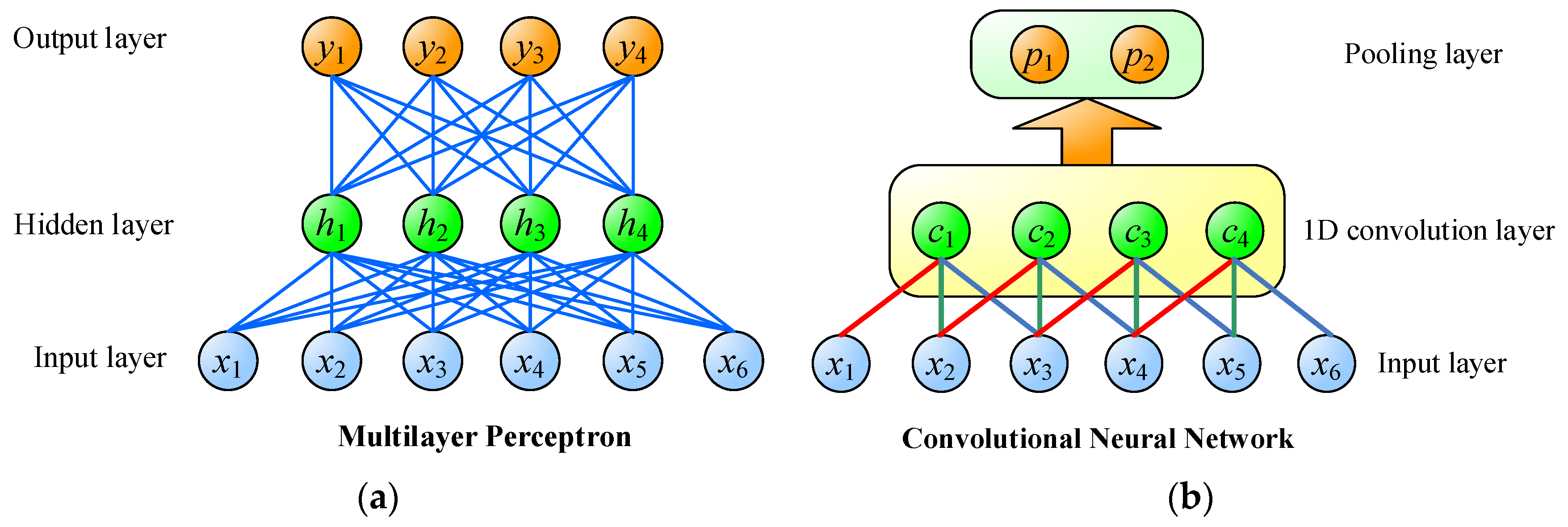
Among the various ANN architectures applied in machine learning problems, the Multilayer Perceptron (MLP) [16] is the most commonly used. The MLP is a fully connected artificial neural network architecture. The structure of MLP is shown in Figure 2a. Generally, the MLP is structured with one input layer, one or more hidden layers, and one output layer. The MLP network presented in Figure 2a is the most common MLP structure, which has only one hidden layer. In the MLP, all the neurons of the previous layer are fully connected to the neurons of the next layer. In Figure 2a, x1, x2, x3, ..., x6 are the neurons of the input layer, h1, h2, h3, h4 are the neurons of the hidden layer, and y1, y2, y3, y4 are the neurons of the output layer. When applied to forecast energy load, the input is the past energy load, and the output is the future energy load. In spite of its simple architecture, MLP provides good results in many applications. The most commonly used algorithm for MLP training is the backpropagation algorithm.
Although the MLP is very good in modelling and pattern recognition, the convolutional neural network (CNN) [17,18,19,20,21,22] which uses the concept of weight sharing provides better accuracy in highly non-linear problems such as energy load forecasting. The one-dimensional convolution and pooling layer are presented in Figure 2b. The lines in the same color signify the same sharing weight, and sets of the sharing weights can be treated as kernels. After the convolution process, the inputs x1, x2, x3, ..., x6 are transformed to the feature maps c1, c2, c3, c4. The next step in Figure 2b is pooling, wherein the feature map of convolution layer is sampled and its dimension is reduced. For instance, in 4 dimensions exist in the feature map in Figure 2b, after the pooling process the number of dimensions is reduced to 2. The process of pooling is an important procedure to extract the important convolution features.
3.2. Long Short-Term Memory
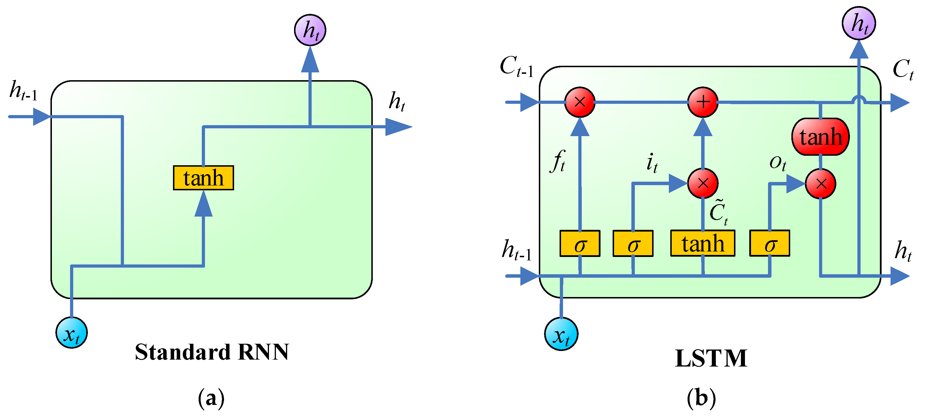
Another popular forecasting method is the recurrent neural network (RNN). RNN is a class of artificial neural network where connections between units form a directed graph along a sequence, as shown in Figure 3a. This structure allows it to exhibit dynamic temporal behavior for a time sequence. Unlike feedforward neural networks, RNNs can use their internal state to process sequences of inputs. Another popular enhanced form of RNN is Long Short Term Memory network (LSTM) [23]. The LSTM is also a recurrent neural network, which has been used to solve many time sequence problems. The structure of LSTM is shown in Figure 3b, and its operation is illustrated by the following equations:
where xt is the network input, and ht is the output of hidden layer, σ denotes the sigmoidal function, Ct is the cell state, and denotes the candidate value of the state. In addition, there are three gates in LSTM: Wf, Wi, Wo, and WC are the weights of forget gate, input gate, output gate, and cell, respectively. bf, bi, bo, and bC are the biases of forget gate, input gate, output gate, and cell, respectively. Whether the input information will be reserved or not is decided by input gate, and the forget gate will determine if the information will be dropped or not. The processing state will be recorded in cell, and the output values of LSTM will be delivered by the output gate. Through this clever design mentioned above, LSTM can learn the long term dependencies from the time sequential data. It is the input gate, is the output gate, and ft is the forget gate. The LSTM is designed for solving the long-term dependency problem. In general, the LSTM provides good forecasting results.
3.3. Batch Normalization
However, in the deep neural network training process, many problems may be encountered. For example, because of the numerous number of layers in deep neural network, when there parameter changes in the previous layer, the output of all subsequent layers will be affected, resulting in frequent corrections from time to time, so there may be poor training efficiency. In addition, if the output value of the neuron already exceeds the proper value range of the activation function itself before passing through the activation function, the neuron may malfunction. However, batch normalization [24] is designed to solve the above mentioned problems. Detailed formulas for batch normalization are shown in(7)–(10).
Here, xi is input value, yi is output value after batch normalization. Where m refers to the mini-batch size, which means that each mini-batch has m inputs. is the total input mean of the same mini-batch. is the input variance of the mini-batch. Next, according to the values of and , we can normalize all xi as , and insert (10) as substitute to acquire yi. Among these γ, β are learning parameters. Through the calculation of batch normalization, the neurons in the deep neural network can be fully utilized and training efficiency could be improved.
4. Hybrid Structured Deep Neural Network
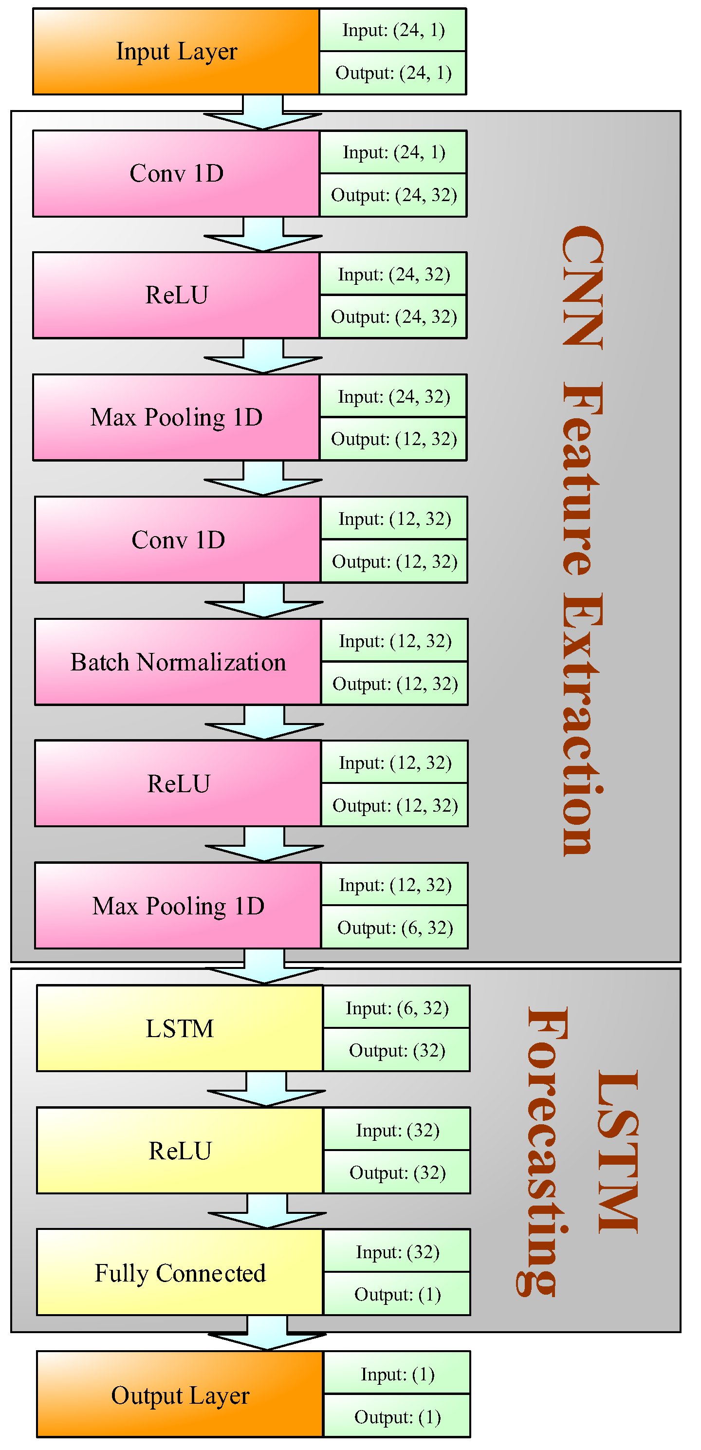
The architecture of the proposed EPNet is shown in Figure 4. EPNet input is the record of electricity price of the past 24 h, and the output is the electricity price of the next hour. Unlike traditional pure CNN or LSTM architectures, the first half of EPNet is CNN and is used for feature extraction, while the latter half is LSTM forecasting, which analyzes the features extracted from CNN and estimate the electricity price for the next point in time. EPNet includes two 1D convolution layers in the CNN segment, in order to improve training efficiency, batch normalization is added after the second convolution layer of EPNet. In general, ReLU is the more widely used activation function, as shown in (11).
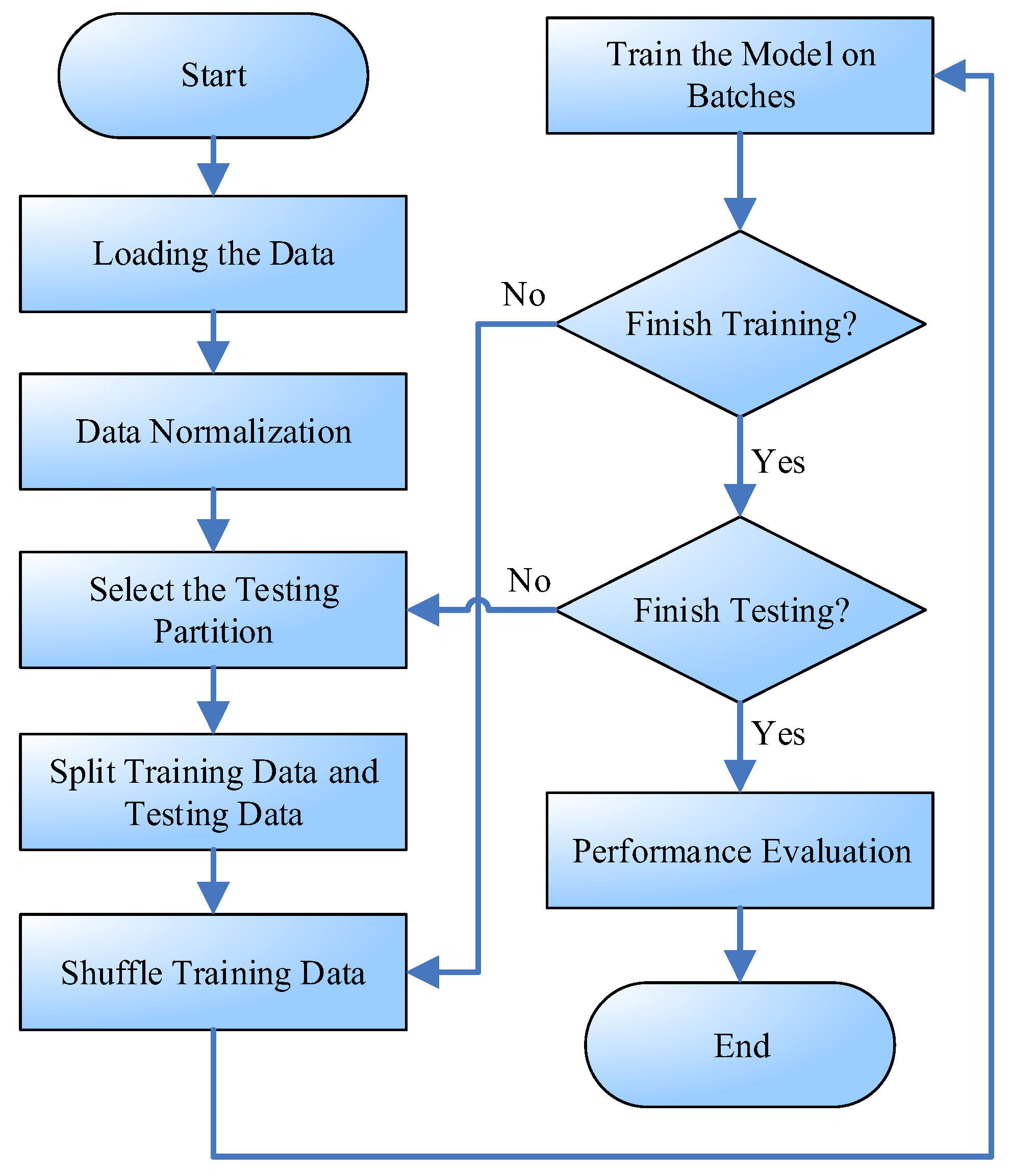
The system flow diagram of the proposed EPNet is shown in Figure 5. In the data preprocessing segment, we first normalize the original dataset, that is to limit the values of all dimentions to the 0 to 1 interval to avoid excess emphasis on a particular dimension during the training process. Next, the normalized data will be split into two parts, the training data and testing data. In order to maintain the fairness of performance evaluation, only training data will be used for training during the training process, and testing data will not be used. After inputting training data into the EPNet, the optimizer will use backpropagation method to adjust the parameters of the EPNet according to the loss value generated. Through various trainings, EPNet forecasting will become more accurate. After EPNet training is complete, we will enter testing data into EPNet and compare the test results with actual data to evaluate the performance of EPNet.
5. Experimental Results
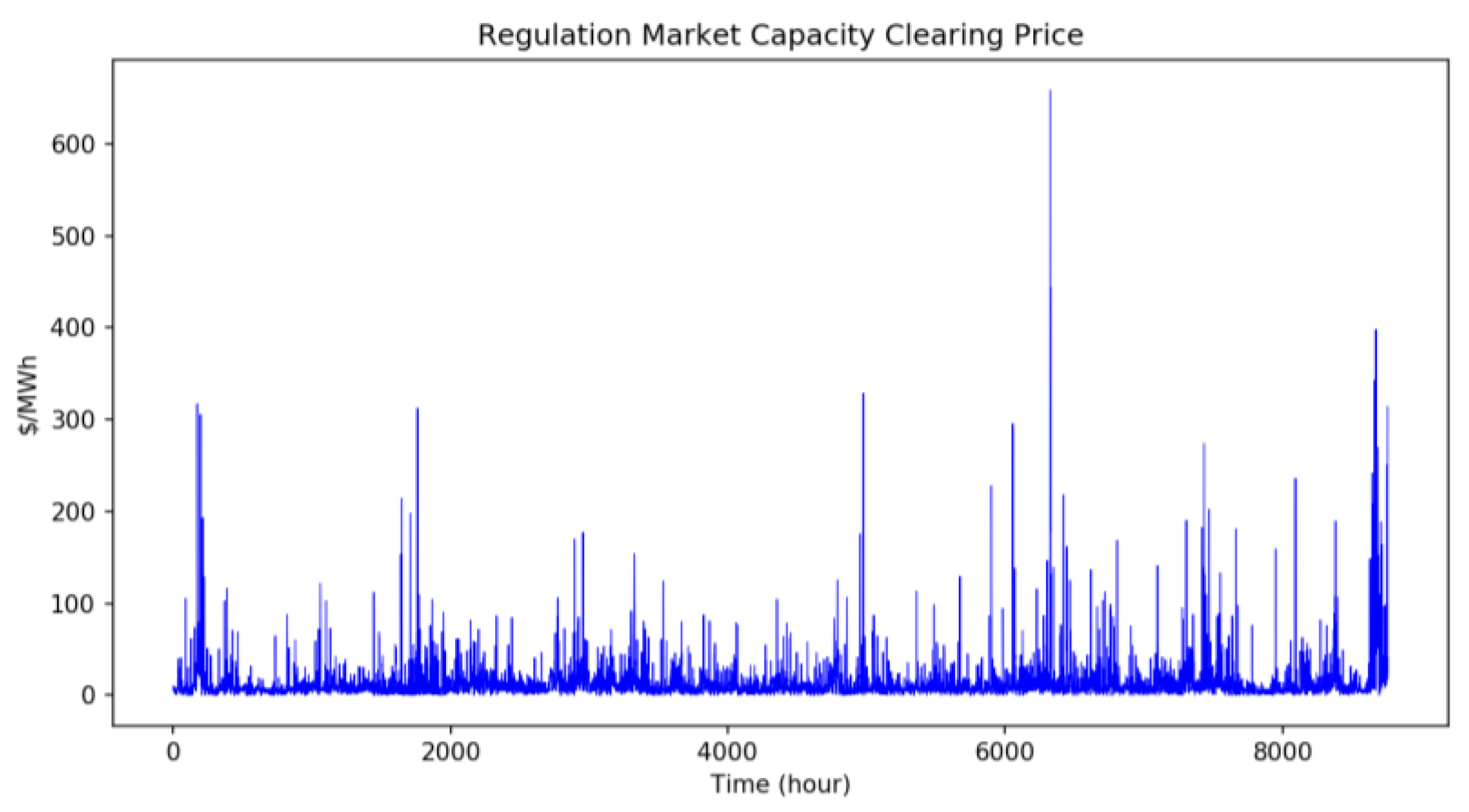
This chapter is described in two parts, the data descriptions segment and the experimental results segment. In order to fully demonstrate the performance of the EPNet proposed in this paper, this chapter includes comparisons between Support Vector Machine (SVM) [25,26,27,28,29,30], Random Forest (RF) [31,32,33,34,35,36], Decision Tree (DT) [37,38,39,40,41,42], MLP, CNN and LSTM. Figure 6 is the Electric Power Markets (PJM) Regulation Zone Preliminary Billing Data [43] used in this experiment, this data records the regulation market capacity clearing price of every half hour in 2017. The dataset provided are republished, with permission, from data collected by the Intercontinental Exchange (ICE), which is updated biweekly. Currently, electricity products can be traded at more than two dozen hubs and delivery points in North America. The data posted under EIA’s agreement with ICE represent eight major electricity hubs. From the figure, we can see that the spread of the regulation market capacity clearing price has a large range, and sudden peak values sometimes occur, which increases the forecasting difficulty for each algorithm.
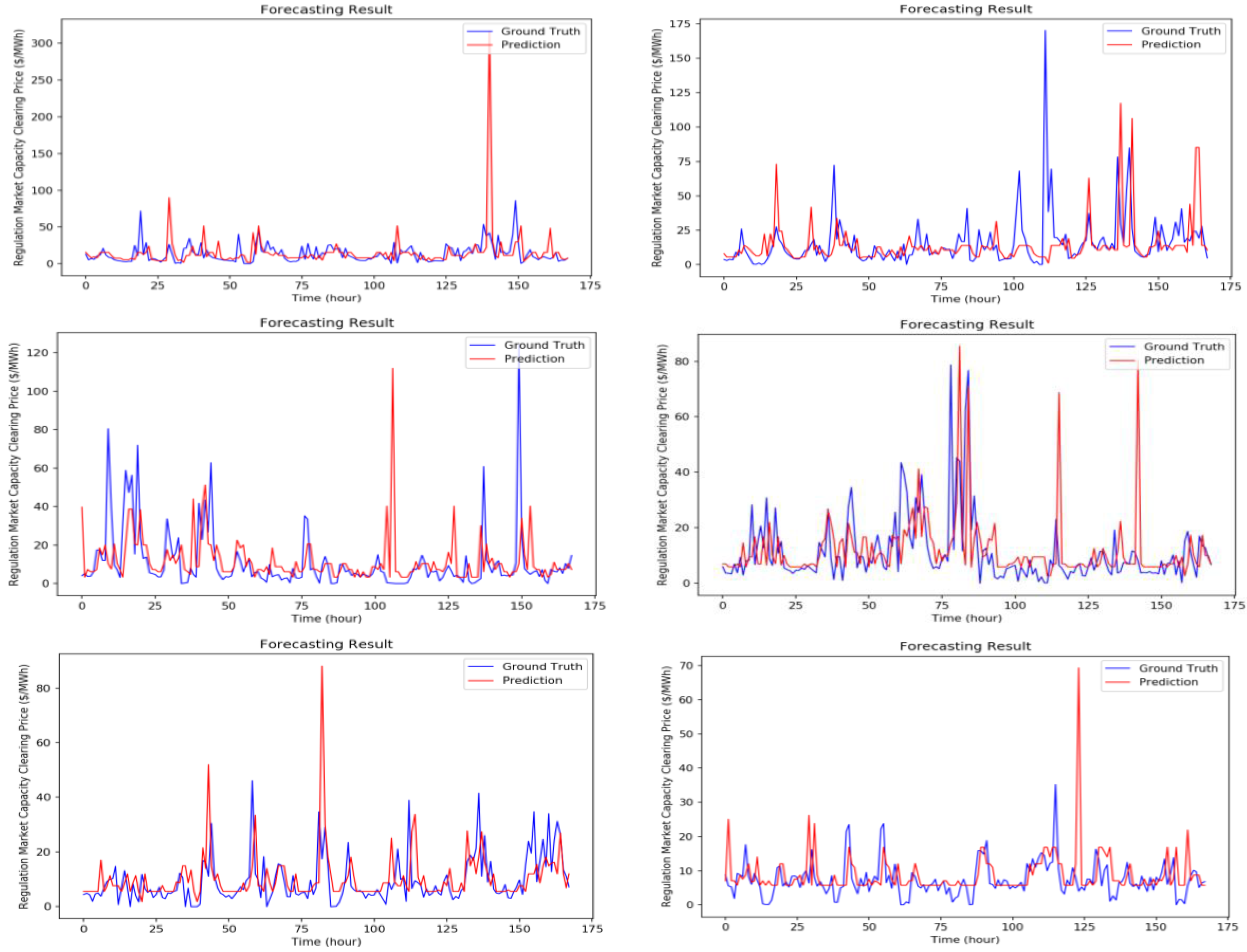
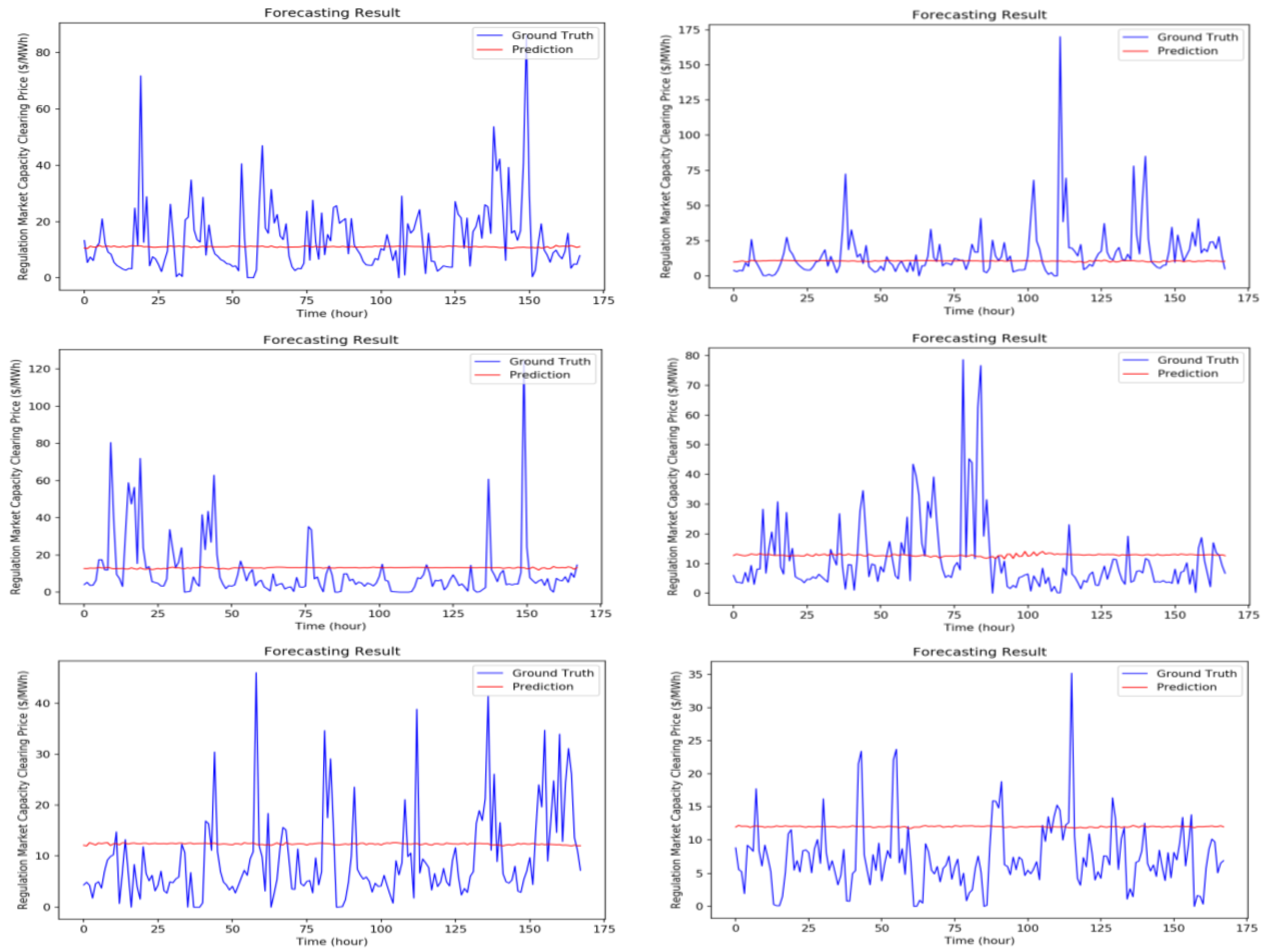
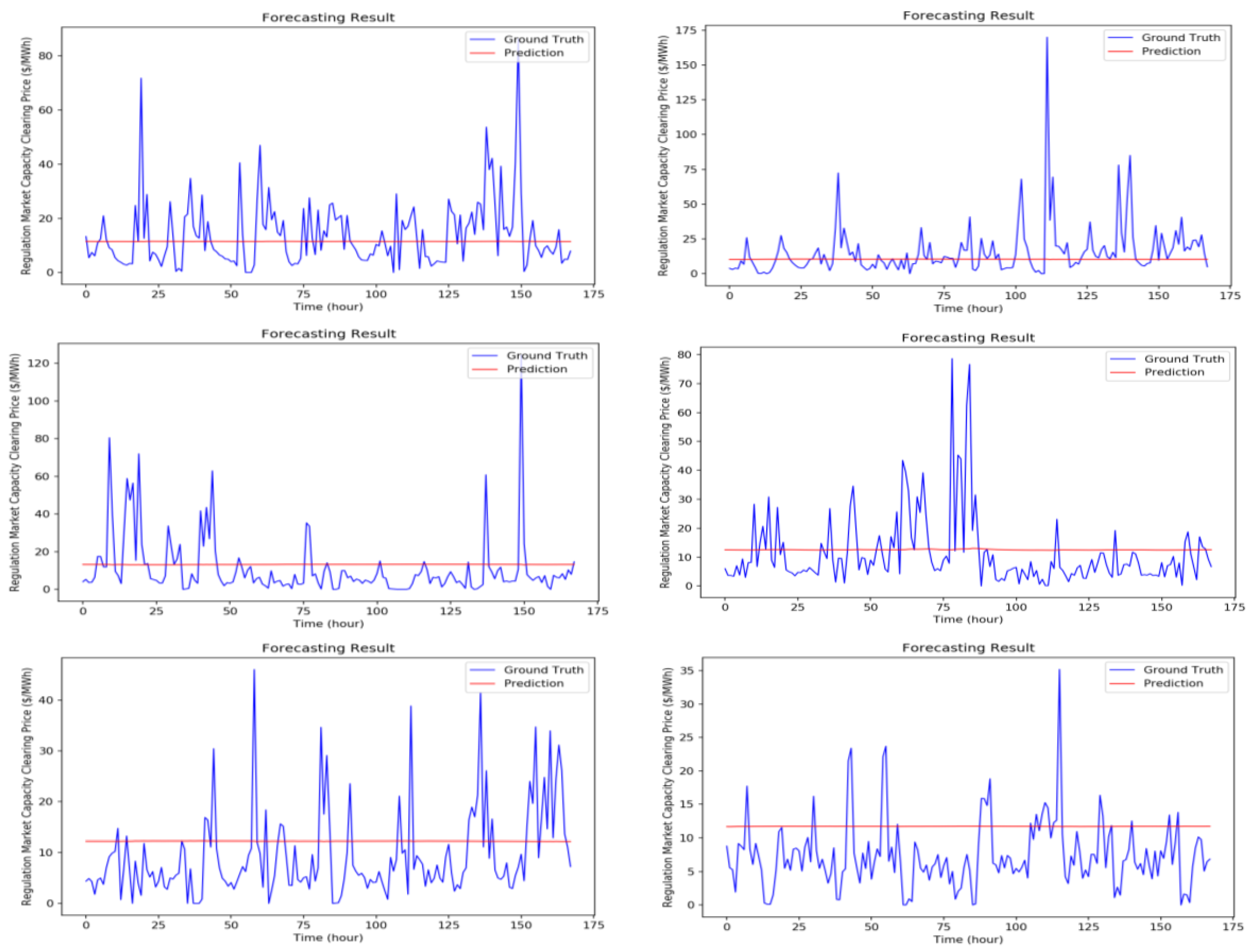
In this experiment, we used two evaluation indicators, the mean absolute error (MAE) and the root-mean-square error (RMSE), the formulas of the indicators are shown in (12) and (13). In order to fully complete the performance test, we selected 10 segments in the database, each segment containing three months’ worth of data as training data, and one month’s worth of data as testing data. Figure 7, Figure 8, Figure 9, Figure 10, Figure 11, Figure 12 and Figure 13 are the forecast results of each algorithm, and Figure 14 shows the comparison of all the algorithms prediction results. From the figure, we can see that SVM performance is slightly weaker in electricity price forecasting, it is unable to grasp the electricity price trend, thus giving highly volatile forecasting results that have almost no matches with the actual data. The performances of DT and RF are slightly better than SVM, they could basically grasp the overall trend of the data, but the error is still quite large, especially with DT, which yields higher miscalculated peak values. If the training is done with basic architectures of MLP, CNN, and LSTM, an almost flat trend is obtained in the forecasting process, the reason being that for MLP, CNN, and LSTM, the electricity price trend is too random to control, so in order to achieve the lowest value of loss during backpropagation, the neural network may estimate the value by averaging, yet this is not the forecast result we want. Among all the methods presented, the best performing algorithm is the one proposed by this paper. Surprisingly, although single MLP, CNN, and LSTM algorithms cannot achieve our goal of forecasting electricity price, but the EPNet which combines CNN and LSTM could not only accurately predict future electricity price value, but is also superior to single MLP, CNN, LSTM forecasting methods. This confirms that EPNet is very effective and accurate in the prediction of electricity prices.
For more complete testing, we extracted 10 segments from the dataset, each segment includes 3 months of training data and 1 month of testing data, and conducted model testing and training on the 10 segments. The test results are shown in Table 1 (MAE) and Table 2 (RMSE). In the MAE ranking, the performance results ranked lowest to highest are EPNet (8.846378), RF (9.201808), DT (9.743163), CNN (9.809469), LSTM (9.82106), MLP (9.860989), SVM (28.98021). In the RMSE ranking, the performance results ranked lowest to highest are EPNet (17.90538), LSTM (18.97729), CNN (18.99075), MLP (18.9891), RF (19.47485), DT (24.88282), SVM (34.28141). From the experiment results, we can see that SVM performed the poorest compared to other algorithms in both MAE and RMSE rankings. The performances of MLP, CNN, LSTM are not as good as that of RF and DT in the MAE assessment, but they performed better than RF and DT in the RMSE ranking. A possible reason may be that on the neural network loss function, the experiment chose to apply the mean squared logarithmic error, so the weight adjustment during backpropagation is beneficial to the RMSE evaluation index. However, overall, the best performance evaluated in either MAE or RMSE or the experiment results from Figure 7, Figure 8, Figure 9, Figure 10, Figure 11, Figure 12, Figure 13 and Figure 14 is the EPNet architecture proposed in this paper.
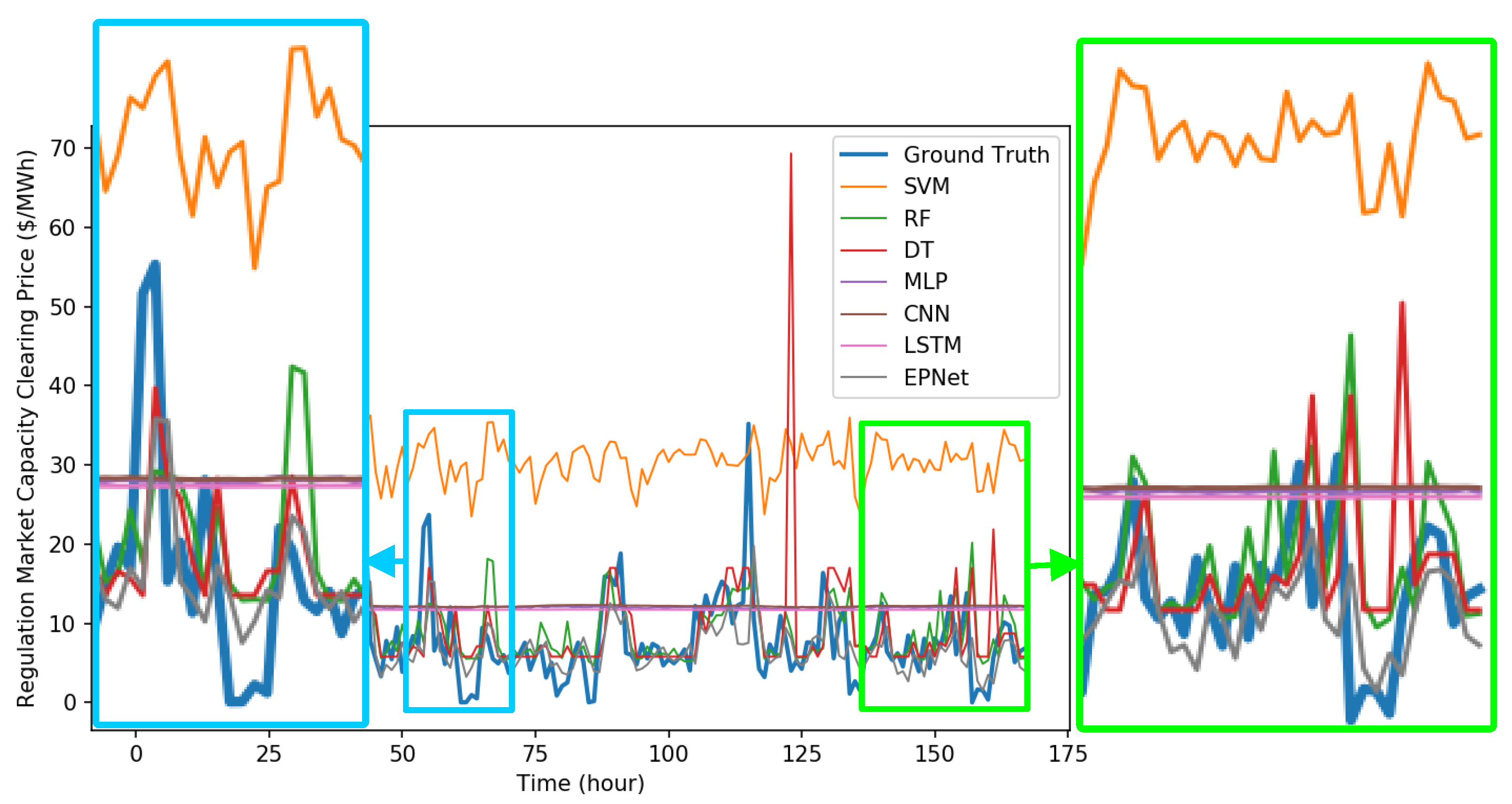
Figure 15 is the detailed performance comparison of the different models. The thick blue line is the actual data, and the lines of other colors are the forecast results calculated by various algorithms. The blue box in Figure 15 shows that the forecast results of SVM almost never matches the actual data, and the forecasts of MLP, CNN, and LSTM do not achieve the expected result. Among all algorithms, the performances of RF, DT and EPNet are better, but RF has misaligned predictions in the second half of the data in the blue box. The green box in Figure 15 shows that SVM almost entirely miscalculated the data trend, and MLP, CNN, and LSTM still do not achieve the expected result, while RF, DT and EPNet performed better. However, DT gave volatile prediction results in the latter half of the data in the green box. Overall, the performances of RF and DT are relatively stable, and the EPNet proposed in this paper has the best performance. Therefore, the ability of EPNet to forecast electricity price is verified in this experiment. According to the characteristics of LSTM, this model is good at handling the time sequence problem, and it has been widely used in many forecasting applications. LSTM is one of the recurrent neural networks which considers the relationship between input values in every time step. However, as shown in (1)–(6), the amount of parameters included in LSTM model also make training much more difficult than that of traditional structures. On the other hand, CNN is another type of neural network. CNN uses the convolution technique to extract important information from the input data. Besides, with an advantage in the “feature extraction” process, CNN can reduce the number of model parameters. As shown in Figure 2, the number of parameters is much fewer than that of the traditional MLP model. In order to solve the main problem of LSTM, in the proposed model, the CNN model is applied first in the feature extraction process. After the most important information has been extracted by CNN, the information will be directly fed into the designed LSTM for the forecasting task. Since the information has been pre-processed by CNN, the analysis of LSTM will be easier. Therefore, estimation performance will be obviously improved, and the conjectures mentioned above are also key points for improvement.
6. Conclusions
This paper proposes a deep neural network model (EPNet) which combines the CNN and the LSTM to forecast future electricity price. EPNet predicts the next hour’s electricity price based on the prices of the previous 24 h. In this experiment, this paper uses PJM Regulation Zone Preliminary Billing Data to perform model training and performance forecast. The paper categorized data into training data and testing data. Training data is used for the training of the model, and testing data which has never been used in the training process will be used to test the model performance on the MAE and RMSE assessments. The performance of EPNet is also compared to that of SVM, RF, DT, MLP, CNN, and LSTM architectures. According to experiment results, compared to traditional machine learning methods, the EPNet proposed in this paper has been proven to have the best forecasting abilities, and its average MAE and RMSE values are the lowest. The feasibility and practicality of proposing a model which combines CNN with LSTM are also confirmed in this paper.
Acknowledgments
This work was performed under auspices of the Ministry of Science and Technology, Taiwan, Republic of China, under Grants MOST 106-2218-E-153-001-MY3 and supported in part by the Jiangxi University of Science and Technology, People’s Republic of China, under Grants jxxjbs18019.
Author Contributions
Ping-Huan Kuo designed this study and collected the dataset. Chiou-Jye Huang wrote the program and designed the CNN-LSTM model. Ping-Huan Kuo and Chiou-Jye Huang contributed in drafted and revised the manuscript.
Conflicts of Interest
The authors declare no conflict of interest.
References
- Nowotarski, J.; Weron, R. Recent advances in electricity price forecasting: A review of probabilistic forecasting. Renew. Sustain. Energy Rev. 2018, 81, 1548–1568. [Google Scholar] [CrossRef]
- Ziel, F.; Weron, R. Day-ahead electricity price forecasting with high-dimensional structures: Univariate vs. multivariate modeling frameworks. Energy Econ. 2018, 70, 396–420. [Google Scholar] [CrossRef]
- Nowotarski, J.; Weron, R. On the importance of the long-term seasonal component in day-ahead electricity price forecasting. Energy Econ. 2016, 57, 228–235. [Google Scholar] [CrossRef]
- Gollou, A.R.; Ghadimi, N. A new feature selection and hybrid forecast engine for day-ahead price forecasting of electricity markets. J. Intell. Fuzzy Syst. 2017, 32, 4031–4045. [Google Scholar] [CrossRef]
- Abedinia, O.; Amjady, N.; Zareipour, H. A New Feature Selection Technique for Load and Price Forecast of Electrical Power Systems. IEEE Trans. Power Syst. 2017, 32, 62–74. [Google Scholar] [CrossRef]
- Bello, A.; Bunn, D.W.; Reneses, J.; Munoz, A. Medium-Term Probabilistic Forecasting of Electricity Prices: A Hybrid Approach. IEEE Trans. Power Syst. 2017, 32, 334–343. [Google Scholar] [CrossRef]
- Lin, W.M.; Gow, H.J.; Tsai, M.T. Electricity price forecasting using enhanced probability neural network. Energy Convers. Manag. 2010, 51, 2707–2714. [Google Scholar] [CrossRef]
- Amjady, N.; Daraeepour, A.; Keynia, F. Day-ahead electricity price forecasting by modified relief algorithm and hybrid neural network. IET Gener. Transm. Distrib. 2010, 4, 432. [Google Scholar] [CrossRef]
- Neupane, B.; Woon, W.; Aung, Z. Ensemble Prediction Model with Expert Selection for Electricity Price Forecasting. Energies 2017, 10, 77. [Google Scholar] [CrossRef]
- Lahmiri, S. Comparing variational and empirical mode decomposition in forecasting day-ahead energy prices. IEEE Syst. J. 2017, 11, 1907–1910. [Google Scholar] [CrossRef]
- González, J.P.; San Roque, A.M.; Pérez, E.A. Forecasting functional time series with a new Hilbertian ARMAX model: Application to electricity price forecasting. IEEE Trans. Power Syst. 2018, 33, 545–556. [Google Scholar] [CrossRef]
- Rafiei, M.; Niknam, T.; Khooban, M.H. Probabilistic Forecasting of Hourly Electricity Price by Generalization of ELM for Usage in Improved Wavelet Neural Network. IEEE Trans. Ind. Inform. 2017, 13, 71–79. [Google Scholar] [CrossRef]
- Benth, F.E.; Benth, J.Š.; Koekebakker, S. Stochastic Modeling of Electricity and Related Markets, 1st ed.; World Scientific: Trenton, NJ, USA, 2010; ISBN 978-981-281-230-8. [Google Scholar]
- An Introduction to Electricity Price Forecasting. Available online: http://energyanalyst.co.uk/an-introduction-to-electricity-price-forecasting/ (accessed on 15 February 2018).
- Hu, L.; Taylor, G.; Wan, H.-B.; Irving, M. A review of short-term electricity price forecasting techniques in deregulated electricity markets. In Proceedings of the 2009 44th International Universities Power Engineering Conference (UPEC 2009), Glasgow, UK, 1–4 September 2009. [Google Scholar]
- White, B.W.; Rosenblatt, F. Principles of Neurodynamics: Perceptrons and the Theory of Brain Mechanisms. Am. J. Psychol. 1963, 76, 705. [Google Scholar] [CrossRef]
- Krizhevsky, A.; Sutskever, I.; Hinton, G.E. ImageNet Classification with Deep Convolutional Neural Networks. Adv. Neural Inf. Process. Syst. 2012, 1–9. [Google Scholar] [CrossRef]
- Qiu, Z.; Chen, J.; Zhao, Y.; Zhu, S.; He, Y.; Zhang, C. Variety Identification of Single Rice Seed Using Hyperspectral Imaging Combined with Convolutional Neural Network. Appl. Sci. 2018, 8, 212. [Google Scholar] [CrossRef]
- Li, C.; Zhou, H. Enhancing the Efficiency of Massive Online Learning by Integrating Intelligent Analysis into MOOCs with an Application to Education of Sustainability. Sustainability 2018, 10, 468. [Google Scholar] [CrossRef]
- Lopez-Martin, M.; Carro, B.; Sanchez-Esguevillas, A.; Lloret, J. Network Traffic Classifier with Convolutional and Recurrent Neural Networks for Internet of Things. IEEE Access 2017, 5, 18042–18050. [Google Scholar] [CrossRef]
- Nam, S.; Park, H.; Seo, C.; Choi, D. Forged Signature Distinction Using Convolutional Neural Network for Feature Extraction. Appl. Sci. 2018, 8, 153. [Google Scholar] [CrossRef]
- An, Q.; Pan, Z.; You, H. Ship Detection in Gaofen-3 SAR Images Based on Sea Clutter Distribution Analysis and Deep Convolutional Neural Network. Sensors 2018, 18, 334. [Google Scholar] [CrossRef] [PubMed]
- Hochreiter, S.; Schmidhuber, J. Long Short-Term Memory. Neural Comput. 1997, 9, 1735–1780. [Google Scholar] [CrossRef] [PubMed]
- Ioffe, S.; Szegedy, C. Batch Normalization: Accelerating Deep Network Training by Reducing Internal Covariate Shift. In Proceedings of the 32nd International Conference on International Conference on Machine Learning (ICML’15), Lile, France, 6–11 July 2015; Volume 37, pp. 448–456. [Google Scholar]
- Suykens, J.A.K.; Vandewalle, J. Least squares support vector machine classifiers. Neural Process. Lett. 1999, 9, 293–300. [Google Scholar] [CrossRef]
- Liu, J.P.; Li, C.L. The short-term power load forecasting based on sperm whale algorithm and wavelet least square support vector machine with DWT-IR for feature selection. Sustainability 2017, 9, 1188. [Google Scholar] [CrossRef]
- Wang, J.; Niu, T.; Wang, R. Research and application of an air quality early warning system based on a modified least squares support vector machine and a cloud model. Int. J. Environ. Res. Public Health 2017, 14, 249. [Google Scholar] [CrossRef] [PubMed]
- Niu, D.; Li, Y.; Dai, S.; Kang, H.; Xue, Z.; Jin, X.; Song, Y. Sustainability Evaluation of Power Grid Construction Projects Using Improved TOPSIS and Least Square Support Vector Machine with Modified Fly Optimization Algorithm. Sustainability 2018, 10, 231. [Google Scholar] [CrossRef]
- Wang, S.; Hae, H.; Kim, J. Development of easily accessible electricity consumption model using open data and GA-SVR. Energies 2018, 11, 373. [Google Scholar] [CrossRef]
- Das, M.; Akpinar, E. Investigation of Pear Drying Performance by Different Methods and Regression of Convective Heat Transfer Coefficient with Support Vector Machine. Appl. Sci. 2018, 8, 215. [Google Scholar] [CrossRef]
- Liaw, A.; Wiener, M. Classification and Regression by randomForest. R News 2002, 2, 18–22. [Google Scholar] [CrossRef]
- Quintana, D.; Sáez, Y.; Isasi, P. Random Forest Prediction of IPO Underpricing. Appl. Sci. 2017, 7, 636. [Google Scholar] [CrossRef]
- MA, J.; Qiao, Y.; Hu, G.; Huang, Y.; Sangaiah, A.K.; Zhang, C.; Wang, Y.; Zhang, R. De-Anonymizing Social Networks With Random Forest Classifier. IEEE Access 2018, 6, 10139–10150. [Google Scholar] [CrossRef]
- Zhu, M.; Xia, J.; Jin, X.; Yan, M.; Cai, G.; Yan, J.; Ning, G. Class Weights Random Forest Algorithm for Processing Class Imbalanced Medical Data. IEEE Access 2018, 6, 4641–4652. [Google Scholar] [CrossRef]
- Hassan, M.; Southworth, J. Analyzing Land Cover Change and Urban Growth Trajectories of the Mega-Urban Region of Dhaka Using Remotely Sensed Data and an Ensemble Classifier. Sustainability 2017, 10, 10. [Google Scholar] [CrossRef]
- Huang, N.; Lu, G.; Xu, D. A permutation importance-based feature selection method for short-term electricity load forecasting using random forest. Energies 2016, 9, 767. [Google Scholar] [CrossRef]
- Safavian, S.R.; Landgrebe, D. A Survey of Decision Tree Classifier Methodology. IEEE Trans. Syst. Man Cybern. 1991, 21, 660–674. [Google Scholar] [CrossRef]
- Rosli, N.; Rahman, M.; Balakrishnan, M.; Komeda, T.; Mazlan, S.; Zamzuri, H. Improved Gender Recognition during Stepping Activity for Rehab Application Using the Combinatorial Fusion Approach of EMG and HRV. Appl. Sci. 2017, 7, 348. [Google Scholar] [CrossRef]
- Huang, N.; Peng, H.; Cai, G.; Chen, J. Power quality disturbances feature selection and recognition using optimal multi-resolution fast S-transform and CART algorithm. Energies 2016, 9, 927. [Google Scholar] [CrossRef]
- Alani, A.Y.; Osunmakinde, I.O. Short-term multiple forecasting of electric energy loads for sustainable demand planning in smart grids for smart homes. Sustainability 2017, 9, 1972. [Google Scholar] [CrossRef]
- Rau, C.-S.; Wu, S.-C.; Chien, P.-C.; Kuo, P.-J.; Chen, Y.-C.; Hsieh, H.-Y.; Hsieh, C.-H.; Liu, H.-T. Identification of Pancreatic Injury in Patients with Elevated Amylase or Lipase Level Using a Decision Tree Classifier: A Cross-Sectional Retrospective Analysis in a Level I Trauma Center. Int. J. Environ. Res. Public Health 2018, 15, 277. [Google Scholar] [CrossRef] [PubMed]
- Rau, C.-S.; Wu, S.-C.; Chien, P.-C.; Kuo, P.-J.; Chen, Y.-C.; Hsieh, H.-Y.; Hsieh, C.-H. Prediction of Mortality in Patients with Isolated Traumatic Subarachnoid Hemorrhage Using a Decision Tree Classifier: A Retrospective Analysis Based on a Trauma Registry System. Int. J. Environ. Res. Public Health 2017, 14, 1420. [Google Scholar] [CrossRef] [PubMed]
- The Electric Power Markets (PJM) Regulation Zone Preliminary Billing Data. Available online: http://www.pjm.com/ (accessed on 15 February 2018).
Figure 1.
The influence factors of electricity price [15].
Figure 1.
The influence factors of electricity price [15].
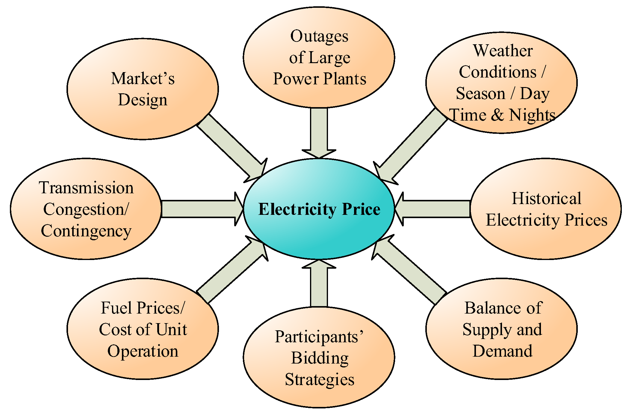
Figure 2.
The comparison of (a) MLP and (b) CNN.

Figure 3.
The comparison of (a) standard RNN and (b) LSTM.

Figure 4.
The architecture of the proposed EPNet.

Figure 5.
The system flowchart of the proposed EPNet.

Figure 6.
PJM Regulation Zone Preliminary Billing Data.

Figure 7.
The forecasting results of SVM.
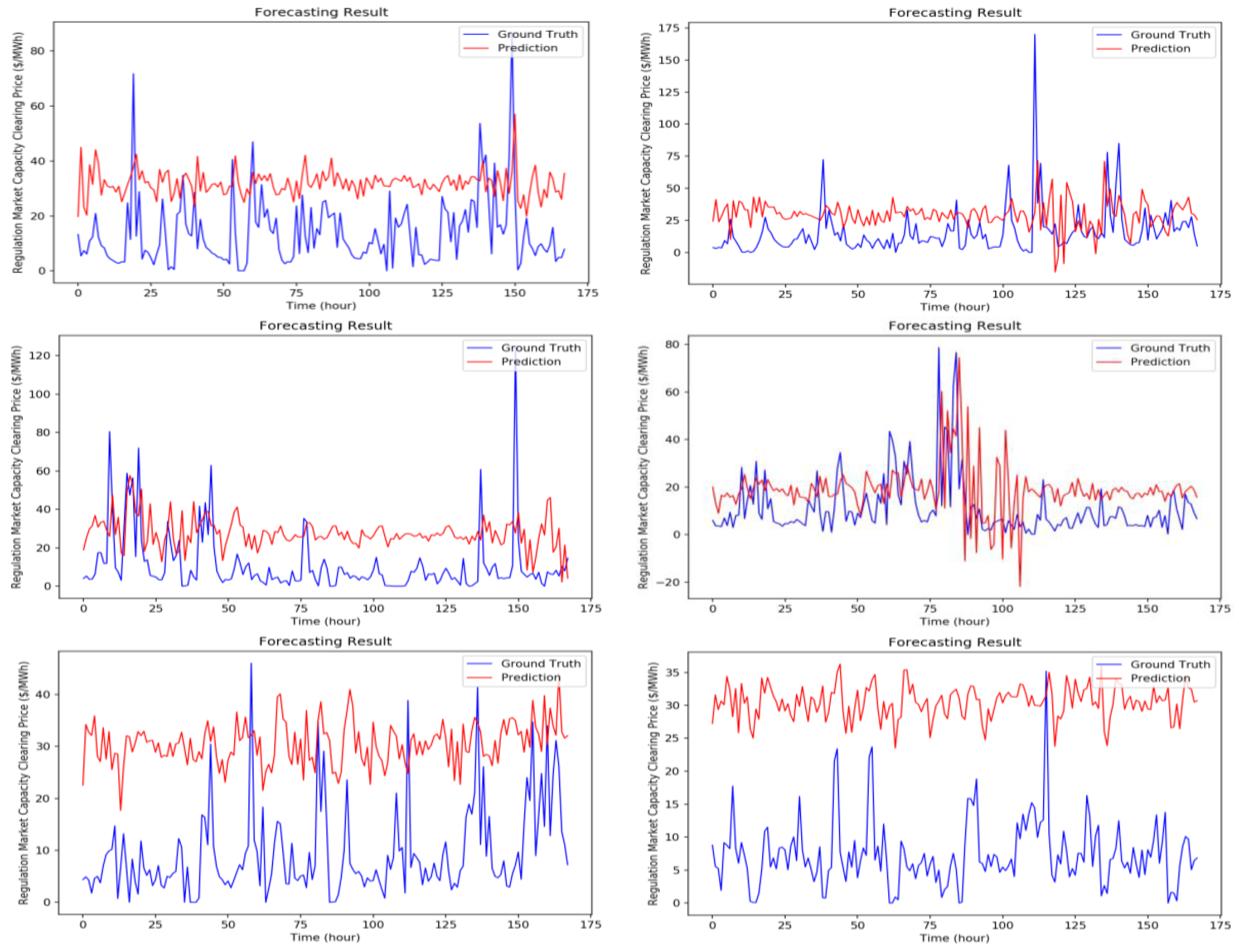
Figure 8.
The forecasting results of random forest.
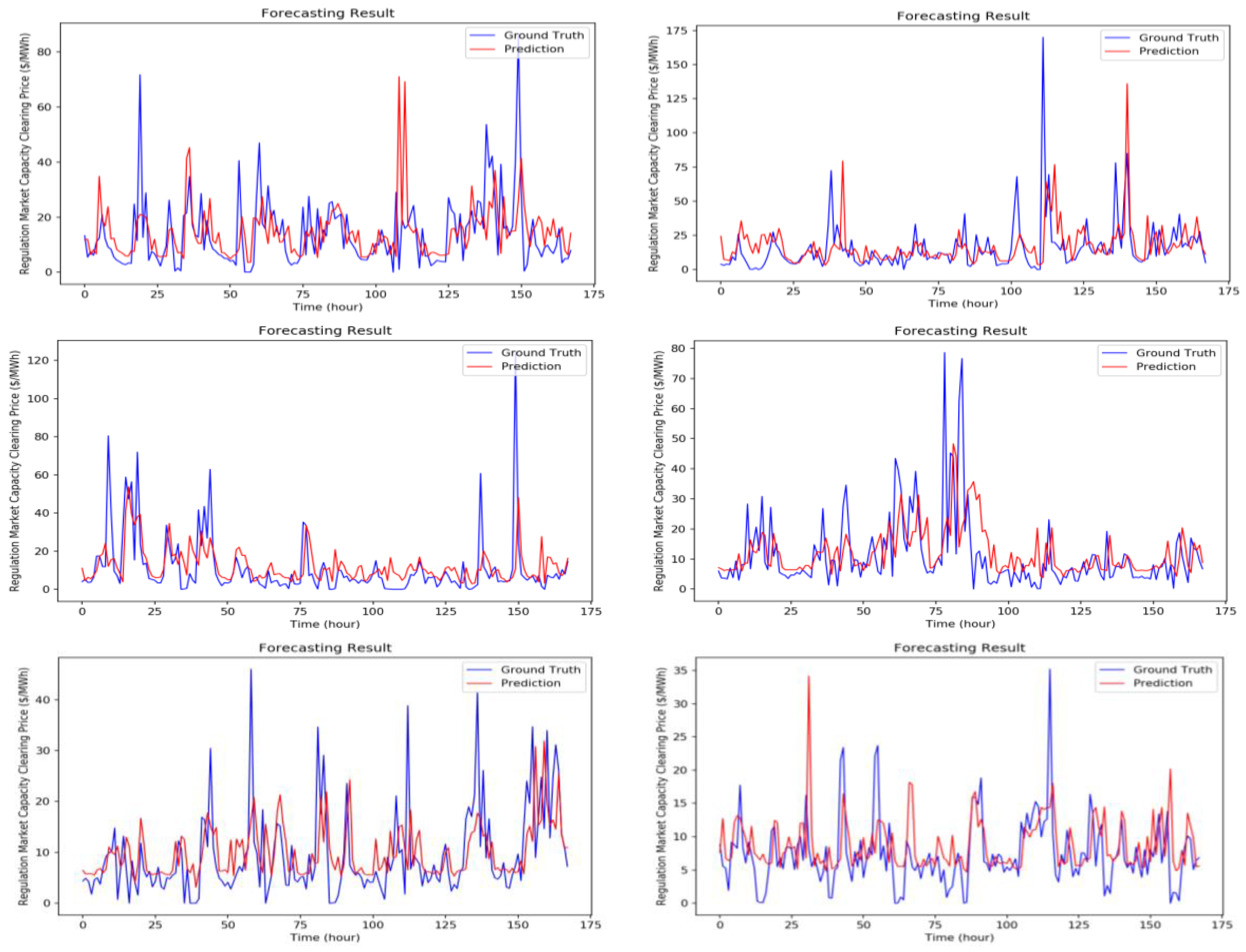
Figure 9.
The forecasting results of decision tree.

Figure 10.
The forecasting results of MLP.

Figure 11.
The forecasting results of CNN.
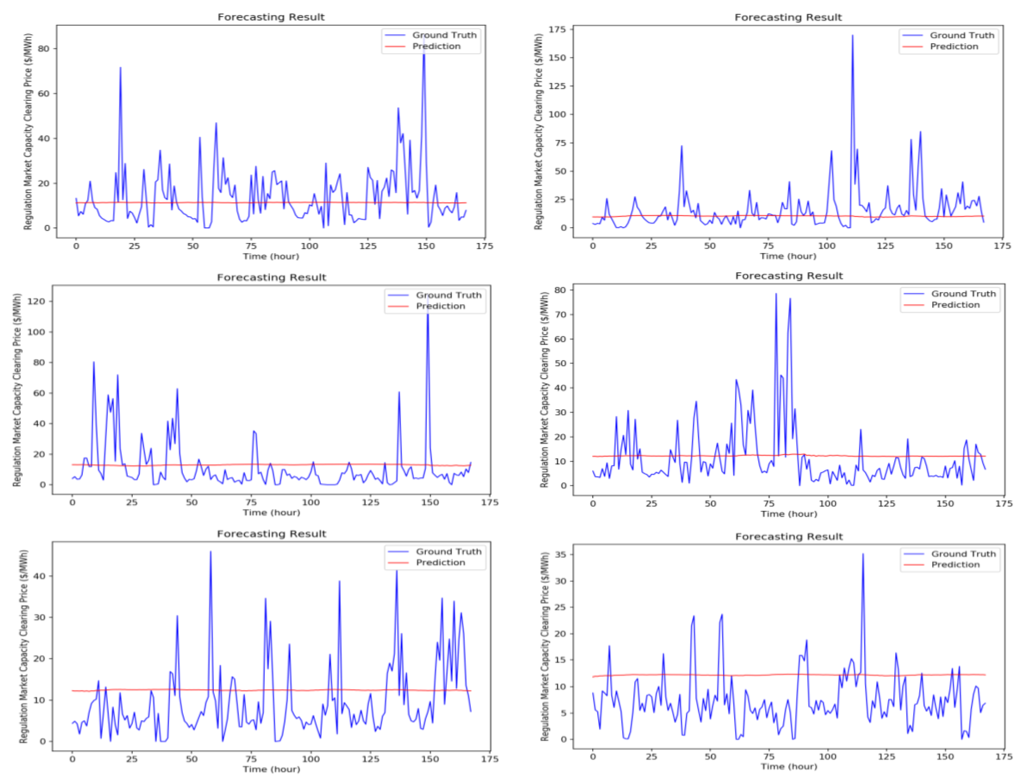
Figure 12.
The forecasting results of LSTM.

Figure 13.
The forecasting results of the proposed EPNet.
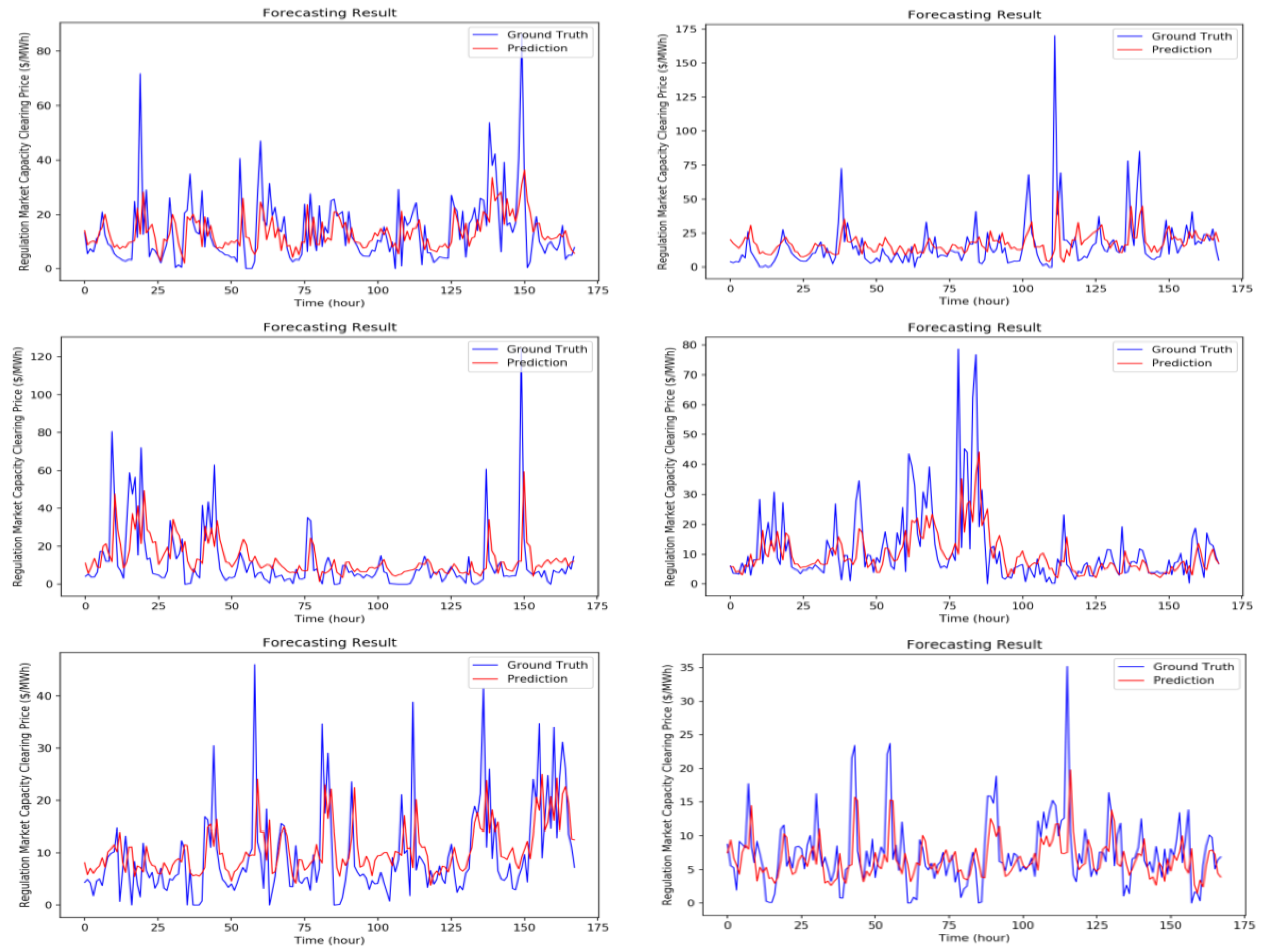
Figure 14.
The comparisons of all the forecasting results.
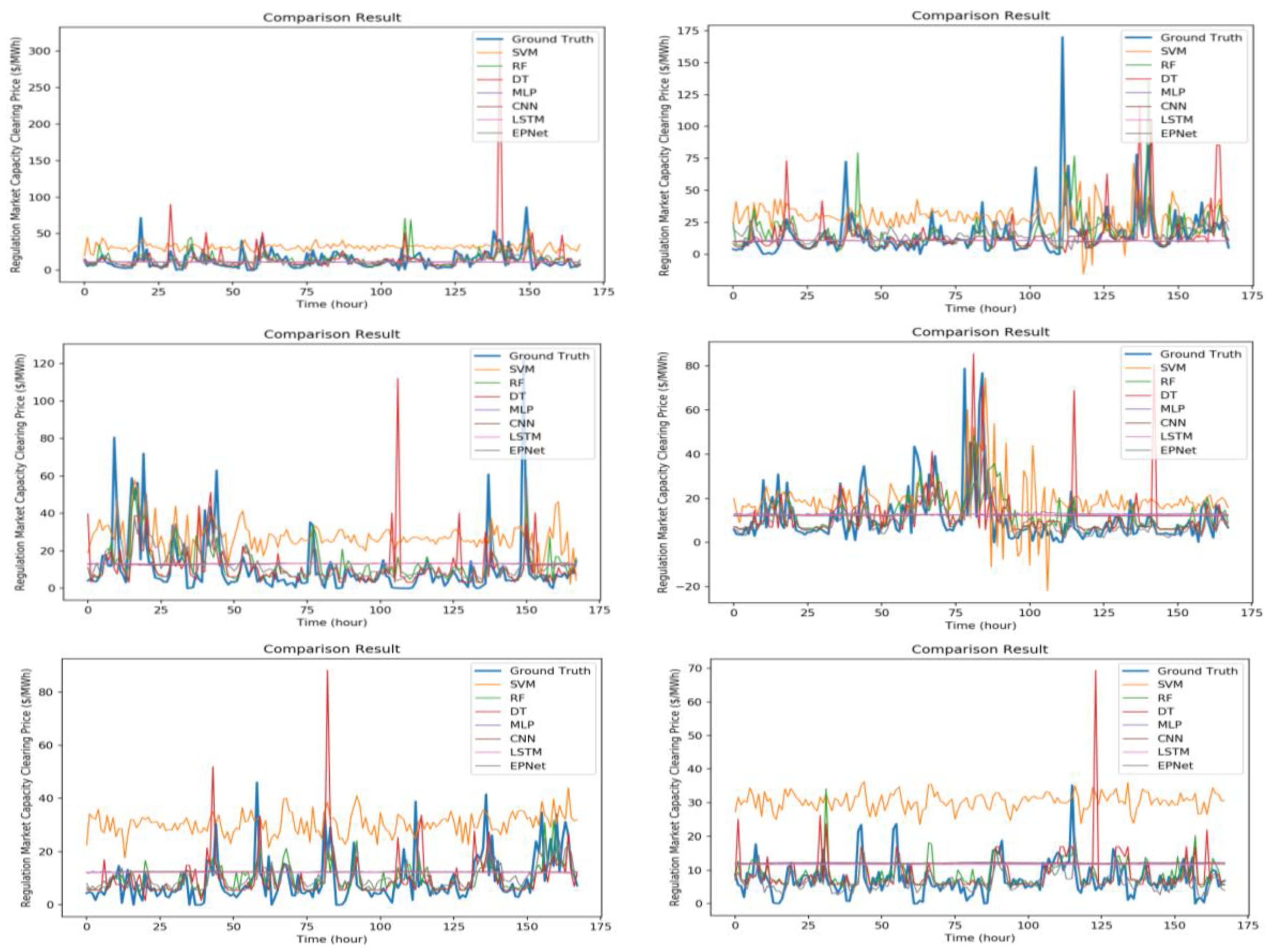
Figure 15.
The comparisons details of forecasting results.


Table 1.
The experimental results in terms of Mean Absolute Error (MAE).
| Test | SVM | RF | DT | MLP | CNN | LSTM | EPNet |
|---|---|---|---|---|---|---|---|
| #1 | 21.39033 | 7.235430 | 7.804850 | 7.43424 | 7.48507 | 7.50518 | 6.64578 |
| #2 | 20.50628 | 10.90374 | 11.26161 | 10.5093 | 10.5437 | 10.4989 | 10.5628 |
| #3 | 19.18263 | 7.668554 | 8.438150 | 9.21527 | 9.19676 | 9.25378 | 7.84723 |
| #4 | 11.67179 | 6.385481 | 7.093340 | 8.06167 | 7.60692 | 7.81942 | 5.58958 |
| #5 | 23.73414 | 7.751149 | 8.375909 | 9.80112 | 9.76736 | 9.72057 | 8.03916 |
| #6 | 22.00405 | 6.055857 | 6.686256 | 7.25569 | 7.28988 | 7.10398 | 5.56724 |
| #7 | 41.34432 | 14.47317 | 15.51438 | 13.6297 | 13.5379 | 13.5496 | 13.7261 |
| #8 | 34.27010 | 10.69618 | 11.52254 | 10.0386 | 9.95490 | 9.94837 | 10.2118 |
| #9 | 42.91338 | 12.00563 | 12.81033 | 11.6585 | 11.6476 | 11.6245 | 11.3043 |
| #10 | 52.78504 | 8.842888 | 7.924259 | 11.0058 | 11.0646 | 11.1863 | 8.96979 |
| Average | 28.98021 | 9.201808 | 9.743163 | 9.860989 | 9.809469 | 9.82106 | 8.846378 |
Table 2.
The experimental results in terms of Root Mean Square Error (RMSE).
| Test | SVM | RF | DT | MLP | CNN | LSTM | EPNet |
|---|---|---|---|---|---|---|---|
| #1 | 22.79050 | 12.33350 | 19.34582 | 11.82432 | 11.76039 | 11.75441 | 10.50514 |
| #2 | 25.06868 | 20.31479 | 20.69246 | 19.61244 | 19.66396 | 19.63171 | 17.22459 |
| #3 | 21.06832 | 12.58604 | 16.24223 | 13.40199 | 13.40107 | 13.39795 | 12.45311 |
| #4 | 14.08044 | 10.81497 | 13.36911 | 11.43035 | 11.19074 | 11.28681 | 10.05318 |
| #5 | 30.12712 | 17.78671 | 20.01475 | 19.25388 | 19.25511 | 19.23331 | 18.23270 |
| #6 | 23.41642 | 10.66788 | 12.99470 | 11.04037 | 11.05200 | 10.98134 | 10.56639 |
| #7 | 66.32881 | 40.86279 | 47.05901 | 42.13376 | 42.24259 | 42.18803 | 39.87986 |
| #8 | 38.79443 | 24.88408 | 42.61376 | 19.51944 | 19.54175 | 19.53222 | 19.06935 |
| #9 | 47.15740 | 25.03586 | 36.95668 | 24.40165 | 24.49525 | 24.41055 | 24.17560 |
| #10 | 53.98195 | 19.46185 | 19.53967 | 17.27284 | 17.30463 | 17.35654 | 16.89385 |
| Average | 34.28141 | 19.47485 | 24.88282 | 18.9891 | 18.99075 | 18.97729 | 17.90538 |
© 2018 by the authors. Licensee MDPI, Basel, Switzerland. This article is an open access article distributed under the terms and conditions of the Creative Commons Attribution (CC BY) license (http://creativecommons.org/licenses/by/4.0/).
Share and Cite
MDPI and ACS Style
Kuo, P.-H.; Huang, C.-J. An Electricity Price Forecasting Model by Hybrid Structured Deep Neural Networks. Sustainability 2018, 10, 1280. https://doi.org/10.3390/su10041280
AMA Style
Kuo P-H, Huang C-J. An Electricity Price Forecasting Model by Hybrid Structured Deep Neural Networks. Sustainability. 2018; 10(4):1280. https://doi.org/10.3390/su10041280
Chicago/Turabian StyleKuo, Ping-Huan, and Chiou-Jye Huang. 2018. "An Electricity Price Forecasting Model by Hybrid Structured Deep Neural Networks" Sustainability 10, no. 4: 1280. https://doi.org/10.3390/su10041280
Note that from the first issue of 2016, this journal uses article numbers instead of page numbers. See further details here.