Inter-Basin Water Transfer Green Supply Chain Equilibrium and Coordination under Social Welfare Maximization

Abstract

The inter-basin water transfer (IBWT) projects have quasi-public-welfare characteristics, whose operations should take into account the water green level (WGL) and social welfare maximization (SWM). This paper explores the interactions between multiple stakeholders of an IBWT green supply chain through the game-theoretic and coordination research approaches considering the government’s subsidy to the WGL improvement under the SWM. The study and its findings complement the IBWT literature in the area of the green supply chain and social welfare maximization modeling. The analytical modeling results with and without considering the SWM are compared. A numerical analysis for a hypothetical IBWT green supply chain is conducted to draw strategic insights from this study. The research results indicate that (1) If the SWM is not considered, coordination strategy could effectively improve the operations performances of the IBWT supply chain and its members, the consumers’ surplus, and the social welfare when compared with the equilibrium strategy; (2) If the SWM is considered, the IBWT green supply chain and its members have a strong intention to adopt the equilibrium strategy to gain more profits, while the government has a strong intention to encourage the IBWT green supply chain and its members to adopt the coordination strategy to maximize social welfare with a smaller public subsidy; (3) The government’s subsidy policy should be designed and provided to encourage the IBWT green supply chain and its members to improve WGL and pursue the SWM, and a subsidy threshold policy can be designed to maximize social welfare with a lower subsidy budget: only when the IBWT green supply chain and its members adopt the coordination strategy can they get a subsidy from the government.

1. Introduction

In the context of global climate change, population growth, and uneven the geographical distribution of natural water resources in many countries and regions, large-scale inter-basin water transfer (IBWT) projects have been constructed and operated worldwide to relieve the water shortage problem; two notable examples are the Central Valley Project in the United States [1,2] and the South-to-North Water Diversion (SNWD) Project in China [3]. However, the ‘World Water Development Report’ released by ‘UN World Water Assessment Plan (WWAP)’ in 2015 pointed out that global water resources waste is still serious, and water abuse behavior is common, either in the water shortage area or in the abundant water area, and revealed that the global water deficit could reach as high as 40% by 2030, according to the current water ratio estimation [4]. Regarding the IBWT projects, the source, channel, and destination of IBWT projects are generally in the densely populated areas and high-incidence of water pollution areas, and continuously maintaining water quality standards, green environmental protection, efficient use of water resources, and ‘clean water corridor’ in this situation is still a big challenge for the IBWT projects in the long run. From the perspective of the operations management of IBWT projects, the quasi-public-goods characteristics of the water resources and the quasi-public-welfare characteristics of the IBWT projects necessitate the government’s appropriate intervention, such as the subsidy to the improvement of water quality, water resources efficiency, and water environment impact to ensure the public would benefit from the green operations of the IBWT projects and maximize the social welfare. According to the current literature regarding green supply chain, the definitions of eco-friendly [5], green level [6], energy saving [7], and greenness index [8] are defined and decided within the framework of green supply chain management. Following their research thinking, we can define water green level (can be abbreviated to WGL) as the comprehensive green level of water quality, water resources efficiency, and water environment impact in the IBWT projects. Hence, how to design an effective government subsidy policy to encourage the IBWT stakeholders to improve the water green level and pursue social welfare maximization (SWM), and how to design an efficient green operations mechanism considering the government subsidy to WGL improvement under the SWM, are urgent problems that need to be solved in the IBWT project. Due to the advantage of taking into account the operations performance, resource efficiency, and environmental impact, the theory and thinking of green supply chain management provides an appropriate perspective for solving the above problems and provides a suitable method for constructing the green operations and the coordination mechanism of the IBWT project in the long run. Therefore, this paper will try to explore the issues of IBWT green supply chain equilibrium and coordination considering the government subsidy to WGL improvement from the perspective of the SWM.

In the following sections, the corresponding literature is reviewed first in Section 2; the notation and assumption for a generic IBWT green supply chain model are defined in Section 3; the IBWT green supply chain equilibrium models considering the government subsidy to WGL improvement under the SWM are developed and analyzed in Section 4; the IBWT green supply chain coordination models considering the government subsidy to WGL improvement under the SWM are developed and analyzed in Section 5; the IBWT supply chain equilibrium and coordination models without considering the government subsidy to WGL improvement and the SWM are analyzed in Section 6; the modeling result comparisons are summarized and discussed in Section 7; the numerical analysis of a hypothetical case for all models is conducted and the results and comparisons are synthesized in Section 8; the management insights and policy implications are then discussed in Section 9; and finally, the research contributions and foresights are synthesized and concluded.

2. Literature Review

The current operations mechanisms of IBWT projects found in literature or practice are mostly developed from the optimization and mathematics programming methods. For example, Li et al. (2017) developed an improved multi-objective optimization model for the operations of south-to-north water diversion (SNWD) project [9]; Zhuan et al. (2017) and Zhuan et al. (2018) developed dynamic programming models for the optimal operation scheduling of pumping station in SNWD project [10,11]; Guo et al. (2012) and Zhu et al. (2017) developed bi-level optimization model for the operations of multi reservoirs in the IBWT projects [12,13]; Wan et al. (2017) developed tri-level programming model for the operations of multi reservoirs in the IBWT projects [14]; Peng et al. (2015) studied multi-reservoir joint operating rule in IBWT projects [15]; Gu et al. (2017) studied simulation and optimization of multi-reservoir operations in IBWT projects [16]; Wan et al. (2018) developed a novel optimization method for multi-reservoir operations in IBWT projects [17]; Wang et al. (2015) studied the optimal operations of bidirectional IBWT projects [18]; Peng et al. (2015) developed optimal operations model with hedging rule for IBWT projects [19]; Mousavi et al. (2017) developed a multi-objective optimization model for the allocation of IBWT projects [20]; Jafarzadegan et al. (2014) developed a stochastic model for the optimal allocation of IBWT projects [21]; Zeng et al. (2014) designed a water transfer triggering mechanism for multi-reservoir operations in IBWT project [22]; and Zhang et al. (2012) developed a negotiation-based multi-objective, multi-party decision-making model for the IBWT Scheme Optimization [23]. These mechanisms could not identify the optimal equilibrium relationships; neither could they coordinate the multiple stakeholders’ benefits in the IBWT projects.

Besides, game theory is applied to identify the equilibrium relationships among stakeholders in the operations management of IBWT projects; for example, Wei et al. (2010) developed a game theory model to analyze water conflicts in the SNWD project [24], Manshadi et al. (2015) developed a game theoretic model for the IBWT system considering both the quantity and quality [25], Rey et al. (2016) designed an innovative option contract for allocating water in the IBWT projects [26], and Sheng et al. (2017) studied the incentive-compatible payments for watershed services along the SNWD Project using the evolutionary game approach [27]. Furthermore, cooperative game theory is applied to balance the individual rationality and the collective rationality in the operations management of IBWT projects; for example, Sadegh et al. (2010) applied the crisp and fuzzy Shapley games to the optimal water allocation in the IBWT system [28], Nikoo et al. (2012) developed an interval parameter cooperative game model for water resources allocation considering the water quality issues in the IBWT system [29], Jafarzadegan et al. (2013) developed a fuzzy variable least core game model for IBWT water resources allocation [30], and Nasiri-Gheidari et al. (2018) developed a robust multi-objective bargaining methodology for IBWT water resource allocation [31].

Taking a supply chain management (SCM) orientation has the advantage of considering both the collective rationality and individual rationality simultaneously in an IBWT project. Recently, SCM concepts and modeling techniques have been applied to the study of the operations management of IBWT projects (especially the South-to-North Water Diversion (SNWD) project in China) such as the definition of the IBWT supply chain, water pricing, water allocation and scheduling, operations performance, and equilibrium and coordination mechanisms. Chen et al. (2013) applied a two-tier pricing scheme to balance water allocation by using a Stackelberg game model for the eastern route of SNWD project, and they concluded that the two-tier pricing scheme is an effective method that can integrate government control and market powers to ensure both the public interest and economic benefits [32]. Wang et al. (2012) studied the pricing and coordinating schemes of the eastern route of SNWD project and discussed the analytical results and their policy implications for the eastern route of SNWD water-resource supply chain [33]. Chen et al. (2012a) developed a decentralized decision model and a centralized decision model with strategic customer behavior using a floating pricing mechanism to construct a coordination mechanism via a revenue-sharing contract [34]. Chen et al. (2012b) further used several game-theoretical models such as Stackelberg game, asymmetric Nash bargaining, etc., when studying the SNWD supply chain [35]. Xu et al. (2012) developed a finite-horizon, periodic-review inventory model with inflow forecasting updates following the Martingale Model of Forecast Evolution (MMFE) to study two-echelon reservoirs in an IBWT project [36]. Obviously, the game and contract theories have been used in the study of the equilibrium decision and benefit coordination mechanism in the IBWT supply chains and the corresponding impact on the operations performance of the IBWT projects.

Nevertheless, an IBWT project typically pursues only the economic goal without considering the water green level (WGL) improvement and the social welfare maximization (SWM). The government subsidy to the WGL improvement and the interactions among the multiple stakeholders in an IBWT green supply chain from a SWM perspective have been rarely investigated in the past. The existing IBWT literatures do not consider the following critical factors: (1) the water green level (WGL) improvement: Due to the quasi-public-goods characteristics of the water resources and the quasi-public-welfare characteristics of the water resources projects, the improvement of water quality, water resources efficiency and water environment impact in the IBWT, projects should be implemented to ensure the public welfare. Therefore, the WGL, which is defined as the comprehensive green level of water quality, water resources efficiency, and water environment impact in the IBWT projects, should be improved; (2) the government’s subsidy policy: Due to the quasi-public-goods characteristics of the water resources and the quasi-public-welfare characteristics of the water resources projects, the government’s subsidy to the WGL improvement is necessary to ensure the public benefits from the IBWT project green operations; (3) the unique structure of an IBWT green supply chain system: An IBWT green supply chain system can be viewed as an ‘embedded’ supply chain structure in which a horizontal green supply chain system is embedded in a vertical green supply chain system (see Figure 1). Due to the embedded supply chain structure characteristics, multiple stakeholders’ optimal decisions and the corresponding operations mechanism in an IBWT green supply chain are different from those of a single water supply system; (4) social welfare maximization: Due to the quasi-public-goods characteristics of the water resources and the quasi-public-welfare characteristics of the water resources projects, not only the goal of economic profit but also the goal of the social welfare should be considered in the green operations of an IBWT project.

To complement the research gaps identified above, a Stackelberg game model and a revenue-sharing contract coordination model for the IBWT green supply chain are developed and solved to explore the optimal operational decisions in an IBWT green supply chain considering the government subsidy to WGL improvement under the SWM. The analytical results are further compared with those without considering the SWM. The numerical analysis is conducted for the analytical models developed in this study to validate the models and gain managerial insights relevant to IBWT practice and policies.

3. IBWT Green Supply Chain Model Structure and Notations

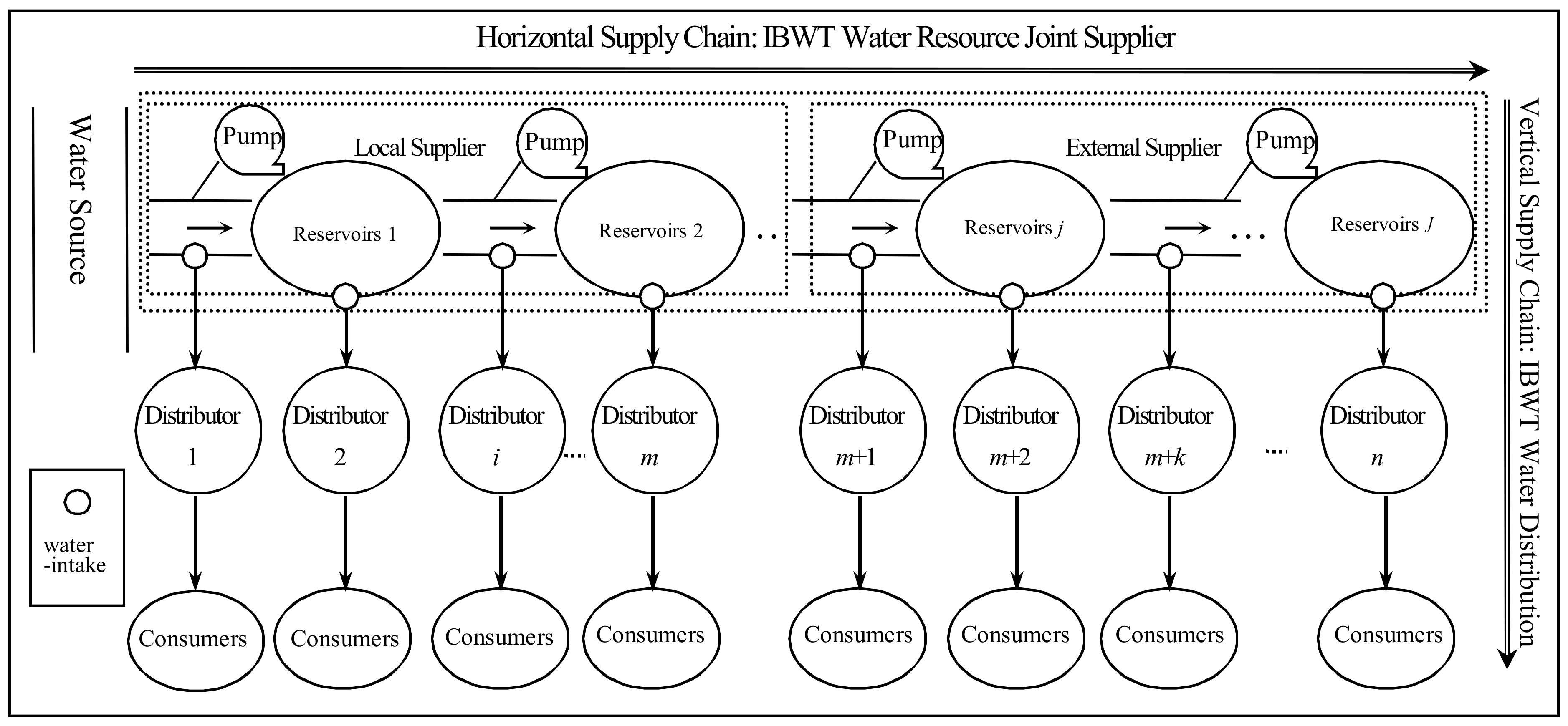
A generic IBWT green supply chain has an ‘embedded’ structure in which a horizontal green supply chain is embedded in a vertical green supply chain (see Figure 1). The horizontal green supply chain is composed of a local supplier and an external supplier, and they serve as a joint IBWT water resources supplier (i.e., an IBWT supplier) via an efficient cooperation mechanism. The water source locates at the territory of the local supplier, and the external supplier relies on the local supplier for her water needs. The local supplier and the external supplier make decisions and take actions such as water allocation, water tariff, etc., subject to the jurisdiction of the central and local water resource authorities. In the vertical green supply chain, the water is supplied from either the water-intake of the river pipeline or the water-intake of the reservoirs to the water resources distributors (i.e., water distributors). The water distributors then sell water to the water resources consumers (i.e., water consumers).

The IBWT supplier is subsidized by the government for its investment cost of water-green-level (WGL) improvement. The transaction characteristics of the IBWT green supply chain are that the local supplier acts as both the water supplier for the external supplier and the water supplier for the water distributors in the local region. That is to say, when the water supply capacity of the local supplier is less than the total water ordering quantity from both the external supplier and the water distributors in the local region, i.e., when the water shortage occurs in the IBWT green supply chain, the local supplier has to allocate the water based on a fair and efficient rule to satisfy the water demand. In this study, we do not consider water shortage problem; rather, we focus on social welfare maximization (SWM) issue, assuming the IBWT water supply capacity is sufficient to meet all downstream demands.

The vertical green supply chain distributes water using the joint IBWT supplier through the multiple water distributors to many water consumers in the service region. The water consumers can only buy water from their regional water distributors due to the fixed physical structure of the water transferring channel and the corresponding facilities and equipment. In rare cases, consumers may buy water from other water distributors through their regional water distributor when they are temporarily out of stock. This paper will not consider the water auction issue among the IBWT distributors during water shortage period. The characteristics of the rigidity of the water distribution in an IBWT green supply chain differentiates it from the general commodity supply chains and how the optimal operations decisions are made.

In Figure 1, the water distributors and the corresponding consumers are indexed by $i=1,2,\dots ,n$. Since the average annual precipitation in an IBWT system is relatively stable (i.e., the extreme climate situation is not considered in this study), its impact on consumer demand and the IBWT system operations can be neglected in the model. The analytical models developed in this study will focus on the key characteristics of the IBWT green supply chain composed by a vertical water distribution system with an embedded horizontal water supply system. We assume there are $m$ distributors supplied by the local supplier and $n-m$ distributors supplied by the external supplier. The water transfer cost from the (i − 1)th water-intake to the ith water-intake within the horizontal green supply chain is $c_i$, and the water transfer cost from the ith water-intake to the ith distributor is $c_{di}$. The fixed cost for the local supplier is $c_{fl}$, and the fixed cost for the external supplier is $c_{fe}$; then, the fixed cost for the IBWT supplier is $c_f=c_{fl}+c_{fe}$. The investment cost of WGL improvement for the IBWT supplier’s ith water-intake is $c_i\left(g_i\right)$ and $c_i\left(g_i\right)=\frac{1}{2}h{g}_i^2$, in which $h$ represents the investment cost factor related to WGL improvement for the IBWT supplier (Basiri et al., 2017;Dai et al., 2017;Liu et al., 2012). The local supplier sells and transfers water resources to the external supplier with the wholesale price $w$ (per m³); the total government subsidy factor (i.e., unit subsidy rate) for the IBWT supplier is $s$ (per m³); the subsidy factor for the ith water-intake is ${\lambda }_{i}s$; and ${\lambda }_i$ is the proportion of the total subsidy factor allocated to the ith water-intake of the IBWT supplier and satisfies ${\displaystyle {\sum }_{i=1}^n{\lambda }_i}=1$.

Two-part tariff system is often applied in the water pricing for the IBWT projects. In Figure 1, the IBWT supplier sells water to the ith distributor with a two-part tariff system, i.e., an entry price (a lump-sum fee) $w_{ei}$ and a usage price (charge per-use or per-unit) $w_i$. The water demand for the consumers in the ith market is $q_i$. The water demand function for the ith water distributor is set as $q_i\left(p_i,g_i\right)=a_i-b{p}_i+\theta g_i$, in which $p_i$ is the retail price of water, $g_i$ is the WGL improvement (which refers to eco-friendly level improvement and quality level improvement of the water resources, which depends on the mutual interaction between the water resources and water environment), $a_i$ is the upper-bound of water demand quantity(when the retail price and the WGL improvement are both zero), $b$ is the reaction extent of the water resources demand with regard to(w.r.t.) the change of the retail price, and $\theta$ is the reaction extent of the water resources demand w.r.t. the change of the WGL improvement. The larger the $b$ value is, the more sensitive the demand is to a change in price. The larger the $\theta$ value is, the more sensitive the demand is to a change in WGL improvement. The inverse water demand function for the ith distributor can be derived as: $p_i\left(q_i,g_i\right)=\frac{1}{b}\left(a_i-q_i+\theta g_i\right)$, $i=1,2,\dots ,n$. Besides, $bh>{\theta }^2$.

The IBWT green supply chain analytical models considering the government subsidy to WGL improvement under the SWM are developed in Section 4 and Section 5, and their optimal conditions/solutions are also solved. The IBWT supply chain analytical models without considering the government subsidy to WGL improvement and the SWM in Section 6 and their optimal solutions are also solved, serving for comparison analysis.

Table 1. Analytical models developed for IBWT green supply chain analysis.

Section	Supply Chain Analysis	Sub-Section	Analytical Model	Theory Applied
4	Equilibrium	Section 4.1	IBWT Vertical Green Supply Chain	Stackelberg Game (SG)
		Section 4.2	IBWT Horizontal Green Supply Chain	Nash Bargaining Game (NBG)
		Section 4.3	IBWT Green Supply Chain with the SWM	SG + NBG + Social Welfare
5	Coordination	Section 5.1	IBWT Vertical Green Supply Chain	Revenue Sharing Contract (RSC)
		Section 5.2	IBWT Horizontal Green Supply Chain	Nash Bargaining Game (NBG)
		Section 5.3	IBWT Green Supply Chain with the SWM	RSC + NBG + Social Welfare
6	Comparison Analysis	Section 6.1	IBWT SC Equilibrium without the SWM	SG + NBG + Social Welfare
		Section 6.2	IBWT SC Coordination without the SWM	RSC + NBG + Social Welfare

lists, in order, these models for clarity purpose.

In Section 4, the IBWT green supply chain equilibrium problems considering the government subsidy to WGL improvement under the SWM are studied. The government’s intention is to subsidize the IBWT supplier in a way such that the social welfare can be maximized in the IBWT green supply chain. In the IBWT vertical green supply chain (Section 4.1), each supply chain member tries to maximize her own profits by playing Stackelberg Game (SG). The players in the embedded IBWT horizontal green supply chain (Section 4.2), i.e., the local and external suppliers, need to decide what wholesale prices, WGL improvement, and quantities of waters need to be set by playing a Nash Bargaining Game (NBG). On this basis, the IBWT green supply chain equilibrium considering the government subsidy to WGL improvement under the SWM can be analyzed in Section 4.3.

In Section 5, the IBWT green supply chain coordination problems, considering the government subsidy to WGL improvement under the SWM, are studied. In the IBWT vertical green supply chain (Section 5.1), the supply chain members cooperate in making pricing and quantity decisions through a revenue sharing contract serving as a coordination mechanism. Similarly, the local and external suppliers in the embedded IBWT horizontal green supply chain (Section 5.2) need to decide the optimal wholesale prices, WGL improvement, and quantity of water by playing a Nash Bargaining Game (NBG). On this basis, the IBWT green supply chain coordination considering the government subsidy to WGL improvement under the SWM can be analyzed in Section 5.3.

In Section 6, the IBWT supply chain equilibrium and coordination without considering the government subsidy to WGL improvement and the SWM are studied, serving for the comparison analysis. For the IBWT supply chain equilibrium (Section 6.1), each supply chain member tries to maximize her own profits by playing Stackelberg Game (SG) in the IBWT vertical supply chain, and the local and external suppliers need to decide what wholesale prices and quantity of water to be set by playing a Nash Bargaining Game (NBG) in the embedded IBWT horizontal supply chain. For the IBWT supply chain coordination (Section 6.2), the supply chain members cooperate in making pricing and quantity decisions through a revenue-sharing contract serving as a coordination mechanism in the IBWT vertical supply chain; the local and external suppliers need to decide the optimal wholesale prices and quantities of waters by playing a Nash Bargaining Game (NBG) in the embedded IBWT horizontal supply chain.

4. IBWT Green Supply Chain Equilibrium with the SWM

4.1. Stackelberg Game between IBWT Supplier and Water Distributors within the IBWT Vertical Green Supply Chain

In the IBWT vertical green supply chain, the optimal problem for the ith distributor is formulated as follows:

$$\underset{p_i}{\max }{\Pi }_{D_i}\left(p_i\right)=\left(p_i-w_i-c_{di}\right)q_i\left(p_i,g_i\right)-w_{ei}$$

(1)

Solving the first-order condition and the second-order derivative of the optimal problem w.r.t. the water retail price $p_i$, respectively, we can obtain the reaction function of the water retail price $p_i$ w.r.t. the water usage price $w_i$ and WGL improvement $g_i$, and the reaction function of ordering quantity $q_i$ w.r.t. the water usage price $w_i$ and WGL improvement $g_i$ as follows:

$$p_i\left(w_i,g_i\right)=\frac{1}{2b}\left(a_i+\theta g_i+b{w}_i+b{c}_{di}\right)$$

(2)

$$q_i\left(w_i,g_i\right)=\frac{1}{2}\left[\left(a_i+\theta g_i\right)-\left(b{w}_i+b{c}_{di}\right)\right]$$

(3)

Plugging $q_i\left(w_i\right)$ into the IBWT supplier’s profit function, we can get the optimal problem for the IBWT supplier as follows:

$$\underset{w_i,g_i}{\max }{\Pi }_S\left(w_i,g_i\right)={\displaystyle {\sum }_{i=1}^n\left[\left(w_i+{\lambda }_{i}s-{\displaystyle {\sum }_{k=1}^i{c}_k}\right)q_i\left(w_i,g_i\right)-\frac{1}{2}h{g}_i^2\right]}+{\displaystyle {\sum }_{i=1}^n{w}_{ei}}-c_f$$

(4)

Solving the first-order condition and the Hesssian matrix of the optimal problem w.r.t. the water usage price $w_i$ and the WGL improvement $g_i$, respectively, when the condition $4bh>{\theta }^2$ holds, we can obtain the reaction function of equilibrium water usage price $w_i^d$ w.r.t. the government subsidy factor $s$ and the reaction function of equilibrium WGL improvement $g_i$ w.r.t. the government subsidy factor $s$ as follows:

$$w_i^d\left(s\right)=\frac{2h}{4bh-{\theta }^2}\left[a_i-b\left(c_{di}+{\displaystyle {\sum }_{k=1}^i{c}_k}-{\lambda }_{i}s\right)\right]+\left({\displaystyle {\sum }_{k=1}^i{c}_k}-{\lambda }_{i}s\right)$$

(5)

$$g_i^d\left(s\right)=\frac{\theta }{4bh-{\theta }^2}\left[a_i-b\left(c_{di}+{\displaystyle {\sum }_{k=1}^i{c}_k}-{\lambda }_{i}s\right)\right]$$

(6)

Plugging $w_i^d\left(s\right)$ and $g_i^d\left(s\right)$ into $p_i\left(w_i\right)$ and $q_i\left(w_i\right)$, we can get the reaction function of equilibrium retail price $p_i^d$ w.r.t. the government subsidy factor $s$ and the reaction function of equilibrium ordering quantity $q_i^d$ w.r.t. the government subsidy factor $s$ as follows:

$$p_i^d\left(s\right)=\frac{3h}{4bh-{\theta }^2}\left[a_i-b\left(c_{di}+{\displaystyle {\sum }_{k=1}^i{c}_k}-{\lambda }_{i}s\right)\right]+\left(c_{di}+{\displaystyle {\sum }_{k=1}^i{c}_k}-{\lambda }_{i}s\right)$$

(7)

$$q_i^d\left(s\right)=\frac{bh}{4bh-{\theta }^2}\left[a_i-b\left(c_{di}+{\displaystyle {\sum }_{k=1}^i{c}_k}-{\lambda }_{i}s\right)\right]$$

(8)

Then, we can get the reaction function of equilibrium profits of IBWT supplier ${\Pi }_S^d$ and the ith distributor ${\Pi }_{D_i}^d$ w.r.t. the government subsidy factor $s$ as follows:

$${\Pi }_S^d\left(s\right)=\frac{h}{2\left(4bh-{\theta }^2\right)}{\displaystyle {\sum }_{i=1}^n{\left[a_i-b\left(c_{di}+{\displaystyle {\sum }_{k=1}^i{c}_k}-{\lambda }_{i}s\right)\right]}^2}+{\displaystyle {\sum }_{i=1}^n{w}_{ei}}-c_f$$

(9)

$${\Pi }_{D_i}^d\left(s\right)=\frac{b{h}^2}{{\left(4bh-{\theta }^2\right)}^2}{\left[a_i-b\left(c_{di}+{\displaystyle {\sum }_{k=1}^i{c}_k}-{\lambda }_{i}s\right)\right]}^2-w_{ei}$$

(10)

4.2. Nash Bargaining between Local Supplier and External Supplier within the IBWT Horizontal Green Supply Chain

This section investigates the decision models in the IBWT horizontal green supply chain of the supply chain equilibrium model through a Nash Bargaining game (superscript d: equilibrium).

Plugging $w_i^d\left(s\right)$ and $q_i^d\left(s\right)$ into the profit functions of the local supplier and the external supplier in the IBWT horizontal supply chain, we can get:

$$\begin{array}{l}{\Pi }_{LS}^d\left(w,s\right)=\frac{h}{2\left(4bh-{\theta }^2\right)}{\displaystyle {\sum }_{i=1}^m{\left[a_i-b\left(c_{di}+{\displaystyle {\sum }_{k=1}^i{c}_k}-{\lambda }_{i}s\right)\right]}^2}+{\displaystyle {\sum }_{i=1}^m{w}_{ei}}-c_{fl}\\ +\frac{bh}{4bh-{\theta }^2}w{\displaystyle {\sum }_{i=m+1}^n\left[a_i-b\left(c_{di}+{\displaystyle {\sum }_{k=1}^i{c}_k}-{\lambda }_{i}s\right)\right]}\end{array}$$

(11)

$$\begin{array}{l}{\Pi }_{ES}^d\left(w,s\right)=\frac{h}{2\left(4b{h}_i-{\theta }^2\right)}{\displaystyle {\sum }_{i=m+1}^n{\left[a_i-b\left(c_{di}+{\displaystyle {\sum }_{k=1}^i{c}_k}-{\lambda }_{i}s\right)\right]}^2}+{\displaystyle {\sum }_{i=m+1}^n{w}_{ei}}-c_{fe}\\ -\frac{bh}{4bh-{\theta }^2}w{\displaystyle {\sum }_{i=m+1}^n\left[a_i-b\left(c_{di}+{\displaystyle {\sum }_{k=1}^i{c}_k}-{\lambda }_{i}s\right)\right]}\end{array}$$

(12)

The Nash Bargaining problem is a classic game theoretic problem developed by Nash (1950) [37] and later expanded by Kalai and Smordinsky (1975) [38]. The Nash bargaining game is a simple two-player game used to model bargaining interactions. In the Nash bargaining game, two players demand a portion of some profit or revenue. If the total amount requested by the players is not larger than that available, both players get their request. If their total request is greater than that available, neither player gets their request. A Nash Bargaining Solution (NBS) is a Pareto efficient solution to a Nash bargaining game, which can be interpreted as a formula that determines a unique outcome for the bargaining situations.

In the Nash Bargaining game, we assume that the status quo (e.g., not reaching agreement and not operating in the market) during the negotiation results in zero profit, i.e., $d_{LS}=d_{ES}=0$ is set to reflect the status quo. The bargaining power of the local supplier τ is set at a fixed value between 0 and 1, i.e., $\tau \in \left(0,1\right)$; the larger the value of τ, the higher the bargaining power of the local supplier will be. Asymmetric NBS to the maximization problem for bargaining over the wholesale price $w$ is as follows [39]:

$$\begin{array}{l}\underset{w}{\max }\pi \left(w\right)={\left[{\Pi }_{LS}^d\left(w,s\right)\right]}^{\tau }{\left[{\Pi }_{ES}^d\left(w,s\right)\right]}^{1-\tau }\\ s.t.{\Pi }_{LS}^d\left(w,s\right)+{\Pi }_{ES}^d\left(w,s\right)={\Pi }_S^d\left(s\right)\\ w>0\end{array}$$

(13)

Solving the first-order condition and the second-order derivative of the optimal problem w.r.t. the wholesale price $w$, respectively, we can obtain the reaction function of bargaining wholesale price $w_d$ w.r.t. the government subsidy factor $s$ as follows:

$$w_d\left(s\right)=\frac{W_d\left(s\right)}{{\displaystyle {\sum }_{i=m+1}^n{q}_i^d\left(s\right)}}$$

(14)

Hereinto,

$$\begin{array}{cc}\hfill W_d\left(s\right)& =\tau \left\{\frac{h}{2\left(4bh-{\theta }^2\right)}{\displaystyle {\sum }_{i=1}^n{\left[a_i-b\left(c_{di}+{\displaystyle {\sum }_{k=1}^i{c}_k}-{\lambda }_{i}s\right)\right]}^2}+{\displaystyle {\sum }_{i=1}^n{w}_{ei}}-c_f\right\}\hfill \\ & -\left\{\frac{h}{2\left(4bh-{\theta }^2\right)}{\displaystyle {\sum }_{i=1}^m{\left[a_i-b\left(c_{di}+{\displaystyle {\sum }_{k=1}^i{c}_k}-{\lambda }_{i}s\right)\right]}^2}+{\displaystyle {\sum }_{i=1}^m{w}_{ei}}-c_{fl}\right\}\hfill \end{array}$$

4.3. IBWT Green Supply Chain Equilibrium with the SWM

According to classical economics theory (Singh & Vives, 1984) [40], the total consumers’ surplus in the IBWT green supply chain can be written as $CS={\displaystyle {\sum }_{i=1}^{n}C{S}_i}=\frac{1}{2b}{\displaystyle {\sum }_{i=1}^n{q}_i^2}$; the total government subsidy is $TS={\displaystyle {\sum }_{i=1}^n{\lambda }_{i}s{q}_i}$. On this basis, we can express the social welfare function SW for the IBWT green supply chain as:

$$SW={\displaystyle {\sum }_{i=1}^n\left[\frac{1}{b}\left(a_i{q}_i-\frac{1}{2}{q}_i^2+\theta g_i{q}_i\right)-\left(c_{di}+{\displaystyle {\sum }_{k=1}^i{c}_k}\right)q_i-\frac{1}{2}h{g}_i^2\right]}-c_f$$

Plugging $q_i^d\left(s\right)$ into the social welfare function for the IBWT green supply chain, the optimal problem for the social welfare of IBWT green supply chain is formulated as follows:

$$\underset{s}{\max }SW\left(s\right)={\displaystyle {\sum }_{i=1}^n\left\{\begin{array}{l}\frac{1}{b}{a}_i{q}_i^d\left(s\right)-\frac{1}{2b}{\left[q_i^d\left(s\right)\right]}^2+\frac{1}{b}\theta g_i^d\left(s\right)q_i^d\left(s\right)\\ -\left(c_{di}+{\displaystyle {\sum }_{k=1}^i{c}_k}\right)q_i^d\left(s\right)-\frac{1}{2}h{\left[g_i^d\left(s\right)\right]}^2\end{array}\right\}}-c_f$$

(15)

Solving the first-order condition and the second-order derivative of the optimal problem w.r.t. the subsidy factor $s$, respectively, when condition $bh>{\theta }^2$ holds, we can obtain the reaction function of optimal subsidy factor $s_d$ w.r.t. the ratio ${\lambda }_i$ as follows:

$$\begin{array}{cc}\hfill s_d\left({\lambda }_i\right)& =\frac{3h\left[a_1-b\left(c_{d1}+{\displaystyle {\sum }_{k=1}^1{c}_k}\right)\right]}{\left(bh-{\theta }^2\right){\lambda }_1}=\cdots =\frac{3h\left[a_i-b\left(c_{di}+{\displaystyle {\sum }_{k=1}^i{c}_k}\right)\right]}{\left(bh-{\theta }^2\right){\lambda }_i}\hfill \\ & =\cdots =\frac{3h\left[a_n-b\left(c_{dn}+{\displaystyle {\sum }_{k=1}^n{c}_k}\right)\right]}{\left(bh-{\theta }^2\right){\lambda }_n}\hfill \end{array}$$

(16)

Combining and solving the above equations with condition ${\displaystyle {\sum }_{i=1}^n{\lambda }_i}=1$, we can obtain the optimal allocation ratio ${\lambda }_i^d$ as follows:

$${\lambda }_i^d=\frac{a_i-b\left(c_{di}+{\displaystyle {\sum }_{k=1}^i{c}_k}\right)}{{\displaystyle {\sum }_{i=1}^n\left[a_i-b\left(c_{di}+{\displaystyle {\sum }_{k=1}^i{c}_k}\right)\right]}}$$

(17)

Obviously, the optimal allocation ratio ${\lambda }_i^d$ equals the maximum potential demand $a_i-b\left(c_{di}+{\displaystyle {\sum }_{k=1}^i{c}_k}\right)$ from the initial water intake to the ith water intake divided by the total maximum potential demand ${\displaystyle {\sum }_{i=1}^n\left[a_i-b\left(c_{di}+{\displaystyle {\sum }_{k=1}^i{c}_k}\right)\right]}$ from the initial water intake to the terminal water intake.

Then, we can obtain the optimal subsidy factor $s_d$ as follows:

$$s_d=\frac{3h}{bh-{\theta }^2}{\displaystyle {\sum }_{i=1}^n\left[a_i-b\left(c_{di}+{\displaystyle {\sum }_{k=1}^i{c}_k}\right)\right]}$$

(18)

Hence, we can get the equilibrium water usage price $w_i^d$, the equilibrium retail price $p_i^d$, the equilibrium WGL improvement $g_i^d$, the equilibrium ordering quantity $q_i^d$, and the bargaining wholesale price $w_d$ under the social welfare optimization as follows (superscript d: equilibrium):

$$w_i^d={\displaystyle {\sum }_{k=1}^i{c}_k}-\frac{h}{bh-{\theta }^2}\left[a_i-b\left(c_{di}+{\displaystyle {\sum }_{k=1}^i{c}_k}\right)\right]$$

(19)

$$p_i^d={\displaystyle {\sum }_{k=1}^i{c}_k}+c_{di}$$

(20)

$$g_i^d=\frac{\theta }{bh-{\theta }^2}\left[a_i-b\left(c_{di}+{\displaystyle {\sum }_{k=1}^i{c}_k}\right)\right]$$

(21)

$$q_i^d=\frac{bh}{bh-{\theta }^2}\left[a_i-b\left(c_{di}+{\displaystyle {\sum }_{k=1}^i{c}_k}\right)\right]$$

(22)

$$w_d=\frac{W_d}{{\displaystyle {\sum }_{i=m+1}^n{q}_i^d}}$$

(23)

Hereinto,

$$\begin{array}{cc}\hfill W_d& =\tau \left\{\frac{h\left(4bh-{\theta }^2\right)}{2{\left(bh-{\theta }^2\right)}^2}{\displaystyle {\sum }_{i=1}^n{\left[a_i-b\left(c_{di}+{\displaystyle {\sum }_{k=1}^i{c}_k}\right)\right]}^2}+{\displaystyle {\sum }_{i=1}^n{w}_{ei}}-c_f\right\}\hfill \\ & -\left\{\frac{h\left(4bh-{\theta }^2\right)}{2{\left(bh-{\theta }^2\right)}^2}{\displaystyle {\sum }_{i=1}^m{\left[a_i-b\left(c_{di}+{\displaystyle {\sum }_{k=1}^i{c}_k}\right)\right]}^2}+{\displaystyle {\sum }_{i=1}^m{w}_{ei}}-c_{fl}\right\}\hfill \end{array}$$

Therefore, we can get the equilibrium profit of the ith distributor ${\Pi }_{D_i}^d$, the equilibrium profit of the IBWT supplier ${\Pi }_S^d$, the equilibrium profit of the IBWT green supply chain ${\Pi }_{SC}^d$, the equilibrium social welfare $S{W}_d$, the corresponding consumers’ surplus $C{S}_d$, and the corresponding government’s total subsidy $T{S}_d$ under the social welfare optimization as follows:

$${\Pi }_{D_i}^d=\frac{b{h}^2}{{\left(bh-{\theta }^2\right)}^2}{\left[a_i-b\left(c_{di}+{\displaystyle {\sum }_{k=1}^i{c}_k}\right)\right]}^2-w_{ei}$$

(24)

$${\Pi }_S^d=\frac{h\left(4bh-{\theta }^2\right)}{2{\left(bh-{\theta }^2\right)}^2}{\displaystyle {\sum }_{i=1}^n{\left[a_i-b\left(c_{di}+{\displaystyle {\sum }_{k=1}^i{c}_k}\right)\right]}^2}+{\displaystyle {\sum }_{i=1}^n{w}_{ei}}-c_f$$

(25)

$${\Pi }_{SC}^d=\frac{h\left(6bh-{\theta }^2\right)}{2{\left(bh-{\theta }^2\right)}^2}{\displaystyle {\sum }_{i=1}^n{\left[a_i-b\left(c_{di}+{\displaystyle {\sum }_{k=1}^i{c}_k}\right)\right]}^2}-c_f$$

(26)

$$S{W}_d=\frac{h}{2\left(bh-{\theta }^2\right)}{\displaystyle {\sum }_{i=1}^n{\left[a_i-b\left(c_{di}+{\displaystyle {\sum }_{k=1}^i{c}_k}\right)\right]}^2}-c_f$$

(27)

$$C{S}_d=\frac{b{h}^2}{2{\left(bh-{\theta }^2\right)}^2}{\displaystyle {\sum }_{i=1}^n{\left[a_i-b\left(c_{di}+{\displaystyle {\sum }_{k=1}^i{c}_k}\right)\right]}^2}$$

(28)

$$T{S}_d=\frac{3b{h}^2}{{\left(bh-{\theta }^2\right)}^2}{\displaystyle {\sum }_{i=1}^n{\left[a_i-b\left(c_{di}+{\displaystyle {\sum }_{k=1}^i{c}_k}\right)\right]}^2}$$

(29)

Obviously, the equilibrium profits of IBWT green supply chain and its members, the social welfare, the consumers’ surplus, and the government’s total subsidy increase as the reaction extent of the water resources demand w.r.t. the change in the WGL improvement increases.

Furthermore, we get the bargaining profits of the local supplier and the external supplier within the IBWT horizontal supply chain ${\Pi }_{LS}^d$ and ${\Pi }_{ES}^d$, and the bargaining profit of the local supplier and the external supplier within the IBWT horizontal green supply chain ${\Pi }_{LS}^d$ and ${\Pi }_{ES}^d$ under the social welfare optimization, as follows:

$${\Pi }_{LS}^d=\tau \left\{\frac{h\left(4bh-{\theta }^2\right)}{2{\left(bh-{\theta }^2\right)}^2}{\displaystyle {\sum }_{i=1}^n{\left[a_i-b\left(c_{di}+{\displaystyle {\sum }_{k=1}^i{c}_k}\right)\right]}^2}+{\displaystyle {\sum }_{i=1}^n{w}_{ei}}-c_f\right\}$$

(30)

$${\Pi }_{ES}^d=\left(1-\tau \right)\left\{\frac{h\left(4bh-{\theta }^2\right)}{2{\left(bh-{\theta }^2\right)}^2}{\displaystyle {\sum }_{i=1}^n{\left[a_i-b\left(c_{di}+{\displaystyle {\sum }_{k=1}^i{c}_k}\right)\right]}^2}+{\displaystyle {\sum }_{i=1}^n{w}_{ei}}-c_f\right\}$$

(31)

In summary, as the bargaining power of the local supplier increases, the local supplier’s net profit will increase, and the external supplier’s net profit will decrease, and vice versa.

5. IBWT Green Supply Chain Coordination with the SWM

5.1. IBWT Vertical Green Supply Chain Coordination under Revenue Sharing Contract

The optimal problem for a centralized IBWT green supply chain is as follows:

$$\underset{p_i,g_i}{\max }{\Pi }_{SC}\left(p_i,g_i\right)={\displaystyle {\sum }_{i=1}^n\left[\left(p_i-c_{di}-{\displaystyle {\sum }_{k=1}^i{c}_k}+{\lambda }_{i}s\right)q_i\left(p_i,g_i\right)-\frac{1}{2}h{g}_i^2\right]}-c_f$$

(32)

Solving the first-order condition and the Hessian matrix of the optimal problem w.r.t. the water retail price $p_i$ and the WGL improvement $g_i$, respectively, when the condition $2bh>{\theta }^2$ holds, we can obtain the reaction functions of optimal water retail price $p_i^c$, the WGL improvement $g_i^c$, and optimal ordering quantity $q_i^c$ w.r.t. the government subsidy factor $s$ as follows:

$$p_i^c\left(s\right)=\frac{1}{2bh-{\theta }^2}\left[h{a}_i+\left(bh-{\theta }^2\right)\left(c_{di}+{\displaystyle {\sum }_{k=1}^i{c}_k}-{\lambda }_{i}s\right)\right]$$

(33)

$$g_i^c\left(s\right)=\frac{\theta }{2bh-{\theta }^2}\left[a_i-b\left(c_{di}+{\displaystyle {\sum }_{k=1}^i{c}_k}-{\lambda }_{i}s\right)\right]$$

(34)

$$q_i^c\left(s\right)=\frac{bh}{2bh-{\theta }^2}\left[a_i-b\left(c_{di}+{\displaystyle {\sum }_{k=1}^i{c}_k}-{\lambda }_{i}s\right)\right]$$

(35)

Therefore, the reaction function of optimal profit of the centralized IBWT green supply chain ${\Pi }_{SC}^c$ w.r.t. the government subsidy factor $s$ is as follows:

$${\Pi }_{SC}^c\left(s\right)=\frac{h}{2\left(2bh-{\theta }^2\right)}{\displaystyle {\sum }_{i=1}^n{\left[a_i-b\left(c_{di}+{\displaystyle {\sum }_{k=1}^i{c}_k}-{\lambda }_{i}s\right)\right]}^2}-c_f$$

(36)

In the IBWT vertical green supply chain coordination model, the IBWT supplier offers the distributors a revenue sharing contract in which the IBWT supplier charges a lower wholesale price $w_i$ to the distributors. The revenue sharing strategy provides a strong incentive to the distributors to buy more water and sell in lower retail prices $p_i$ to promote more demand on water $q_i$. The distributors either accept or reject the contract. If the distributors accept, they will share a proportion of their net revenues and investment costs of WGL improvement ϕ to the IBWT supplier in return. In other words, ϕ is the revenue-cost keeping rate of the distributors and 0 ≤ ϕ ≤ 1. The distributors will share a fraction of his net revenue and investment costs of WGL improvement (1 − ϕ) to the IBWT supplier; the transferring revenue and cost from the ith distributor to the IBWT supplier is $T_i=\left(1-\varphi \right)\left[\left(p_i-c_{di}\right)q_i\left(p_i,g_i\right)\right]+\frac{1}{2}\varphi h{g}_i^2$. Hence, the ith distributor’s profit function and the IBWT supplier’s profit function are as follows:

$${\Pi }_{D_i}=\left(p_i-w_i-c_{di}\right)q_i\left(p_i,g_i\right)-w_{ei}-T_i$$

$${\Pi }_S={\displaystyle {\sum }_{i=1}^n\left[\left(w_i+{\lambda }_{i}s-{\displaystyle {\sum }_{k=1}^i{c}_k}\right)q_i\left(p_i,g_i\right)+T_i\right]}+{\displaystyle {\sum }_{i=1}^n{w}_{ei}}-c_f$$

Under the revenue-cost sharing contract, the ith distributor’s optimal problem is formulated as follows:

$$\underset{p_i}{\max }{\Pi }_{D_i}\left(p_i\right)=\left(\varphi p_i-w_i-\varphi c_{di}\right)q_i\left(p_i,g_i\right)-\frac{1}{2}\varphi h{g}_i^2-w_{ei}$$

(37)

Solving the first-order condition and the second-order derivative of the optimal problem w.r.t. the water retail price $p_i$ respectively, we can obtain the reaction function of the water retail price $p_i$ w.r.t. the water usage price $w_i$, and the reaction function of ordering quantity $q_i$ w.r.t. the water usage price $w_i$, as follows:

$$p_i^d\left(w_i,g_i\right)=\frac{1}{2b}\left(a_i+b{c}_{di}+\theta g_i\right)+\frac{1}{2\varphi }{w}_i$$

Plugging $g_i^c\left(s\right)$ into $p_i^d\left(w_i,g_i\right)$, we can obtain

$$p_i^d\left(w_i,g_i^c\left(s\right)\right)=\frac{1}{2bh-{\theta }^2}\left[h{a}_i-\frac{1}{2}{\theta }^2\left(c_{di}+{\displaystyle {\sum }_{k=1}^i{c}_k}-{\lambda }_{i}s\right)\right]+\frac{1}{2}{c}_{di}+\frac{1}{2\varphi }{w}_i$$

(38)

Under the revenue sharing contract, to achieve the IBWT green supply chain coordination, it is necessary to achieve the coordinated condition $p_i^d\left(w_i,g_i^c\left(s\right)\right)=p_i^c\left(s\right)$. Then, we have the coordinated wholesale price $w_i^c\left(s\right)=\varphi \left({\displaystyle {\sum }_{k=1}^i{c}_k}-{\lambda }_{i}s\right)$ for the IBWT supplier.

Therefore, the reaction function of optimal profit of the IBWT supplier ${\Pi }_S^c$ and the distributors’ ${\Pi }_{D_i}^c$ w.r.t. the government subsidy factor $s$ under the revenue sharing contract are shown below:

$${\Pi }_S^c\left(s\right)=\frac{\left(1-\varphi \right)h}{2\left(2bh-{\theta }^2\right)}{\displaystyle {\sum }_{i=1}^n{\left[a_i-b\left(c_{di}+{\displaystyle {\sum }_{k=1}^i{c}_k}-{\lambda }_{i}s\right)\right]}^2}+{\displaystyle {\sum }_{i=1}^n{w}_{ei}}-c_f$$

(39)

$${\Pi }_{D_i}^c\left(s\right)=\frac{\varphi h}{2\left(2bh-{\theta }^2\right)}{\left[a_i-b\left(c_{di}+{\displaystyle {\sum }_{k=1}^i{c}_k}-{\lambda }_{i}s\right)\right]}^2-w_{ei}$$

(40)

Obviously, as the revenue-cost keeping rate ϕ increases, the water distributors’ net profit increases, and the IBWT supplier’s net profit decreases.

5.2. Nash Bargaining between Local Supplier and External Supplier within the IBWT Horizontal Green Supply Chain

This section investigates the decision models in the IBWT horizontal green supply chain of the supply chain coordination model through a Nash Bargaining game (superscript c: coordination).

Plugging $w_i^c$ and $q_i^c\left(s\right)$ into the profit functions of the local supplier and the external supplier in the IBWT horizontal green supply chain, we can get

$$\begin{array}{cc}\hfill {\Pi }_{LS}^c\left(w,s\right)& =\frac{\left(1-\varphi \right)h}{2\left(2bh-{\theta }^2\right)}{\displaystyle {\sum }_{i=1}^m{\left[a_i-b\left(c_{di}+{\displaystyle {\sum }_{k=1}^i{c}_k}-{\lambda }_{i}s\right)\right]}^2}+{\displaystyle {\sum }_{i=1}^m{w}_{ei}}-c_{fl}\hfill \\ & +\frac{bh}{2bh-{\theta }^2}w{\displaystyle {\sum }_{i=m+1}^n\left[a_i-b\left(c_{di}+{\displaystyle {\sum }_{k=1}^i{c}_k}-{\lambda }_{i}s\right)\right]}\hfill \end{array}$$

(41)

$$\begin{array}{cc}\hfill {\Pi }_{ES}^c\left(w,s\right)& =\frac{\left(1-\varphi \right)h}{2\left(2bh-{\theta }^2\right)}{\displaystyle {\sum }_{i=m+1}^n{\left[a_i-b\left(c_{di}+{\displaystyle {\sum }_{k=1}^i{c}_k}-{\lambda }_{i}s\right)\right]}^2}+{\displaystyle {\sum }_{i=m+1}^n{w}_{ei}}-c_{fe}\hfill \\ & -\frac{bh}{2bh-{\theta }^2}w{\displaystyle {\sum }_{i=m+1}^n\left[a_i-b\left(c_{di}+{\displaystyle {\sum }_{k=1}^i{c}_k}-{\lambda }_{i}s\right)\right]}\hfill \end{array}$$

(42)

Likewise, asymmetric NBS to the maximization problem for bargaining over the wholesale price $w$ is as follows:

$$\begin{array}{l}\underset{w}{\max }\pi \left(w\right)={\left[{\Pi }_{LS}^c\left(w,s\right)\right]}^{\tau }{\left[{\Pi }_{ES}^c\left(w,s\right)\right]}^{1-\tau }\\ s.t.{\Pi }_{LS}^c\left(w,s\right)+{\Pi }_{ES}^c\left(w,s\right)={\Pi }_S^c\left(s\right)\\ w>0\end{array}$$

(43)

Solving the first-order condition and the second-order derivative of the optimal problem w.r.t. the wholesale price $w$, respectively, we can obtain the reaction function of bargaining wholesale price $w_c$ w.r.t. the government subsidy factor $s$ as follows:

$$w_c\left(s\right)=\frac{W_c\left(s\right)}{{\displaystyle {\sum }_{i=m+1}^n{q}_i^c\left(s\right)}}$$

(44)

Hereinto,

$$\begin{array}{cc}\hfill w_c\left(s\right)& =\tau \left[\frac{\left(1-\varphi \right)h}{2\left(2bh-{\theta }^2\right)}{\displaystyle {\sum }_{i=1}^n{\left[a_i-b\left(c_{di}+{\displaystyle {\sum }_{k=1}^i{c}_k}-{\lambda }_{i}s\right)\right]}^2}+{\displaystyle {\sum }_{i=1}^n{w}_{ei}}-c_f\right]\hfill \\ & -\left[\frac{\left(1-\varphi \right)h}{2\left(2bh-{\theta }^2\right)}{\displaystyle {\sum }_{i=1}^m{\left[a_i-b\left(c_{di}+{\displaystyle {\sum }_{k=1}^i{c}_k}-{\lambda }_{i}s\right)\right]}^2}+{\displaystyle {\sum }_{i=1}^m{w}_{ei}}-c_{fl}\right]\hfill \end{array}$$

5.3. IBWT Green Supply Chain Coordination with the SWM

Likewise, we express the social welfare function SW for the IBWT green supply chain as $SW={\displaystyle {\sum }_{i=1}^n\left[\frac{1}{b}\left(a_i{q}_i-\frac{1}{2}{q}_i^2+\theta g_i{q}_i\right)-\left(c_{di}+{\displaystyle {\sum }_{k=1}^i{c}_k}\right)q_i-\frac{1}{2}h{g}_i^2\right]}-c_f$. Plugging $q_i^c\left(s\right)$ into the social welfare function for the IBWT green supply chain, the optimal problem for the social welfare of IBWT green supply chain is formulated as follows:

$$\underset{s}{\max }SW\left(s\right)={\displaystyle {\sum }_{i=1}^n\left\{\begin{array}{l}\frac{1}{b}{a}_i{q}_i^c\left(s\right)-\frac{1}{2b}{\left[q_i^c\left(s\right)\right]}^2+\frac{1}{b}\theta g_i^c\left(s\right)q_i^c\left(s\right)\\ -\left(c_{di}+{\displaystyle {\sum }_{k=1}^i{c}_k}\right)q_i^c\left(s\right)-\frac{1}{2}h{\left[g_i^c\left(s\right)\right]}^2\end{array}\right\}}-c_f$$

(45)

Solving the first-order condition and the second-order derivative of the optimal problem w.r.t. the subsidy factor $s$, respectively, when the condition $bh>{\theta }^2$ holds, we can obtain the reaction function of optimal subsidy factor $s_c$ w.r.t. the ratio ${\lambda }_i$ as follows:

$$\begin{array}{cc}\hfill s_c\left({\lambda }_i\right)& =\frac{h\left[a_1-b\left(c_{d1}+{\displaystyle {\sum }_{k=1}^1{c}_k}\right)\right]}{\left(bh-{\theta }^2\right){\lambda }_1}=\cdots =\frac{h\left[a_i-b\left(c_{di}+{\displaystyle {\sum }_{k=1}^i{c}_k}\right)\right]}{\left(bh-{\theta }^2\right){\lambda }_i}\hfill \\ & =\cdots =\frac{h\left[a_n-b\left(c_{dn}+{\displaystyle {\sum }_{k=1}^n{c}_k}\right)\right]}{\left(bh-{\theta }^2\right){\lambda }_n}\hfill \end{array}$$

(46)

Combining and solving the above equations with the condition ${\displaystyle {\sum }_{i=1}^n{\lambda }_i}=1$, we can obtain the optimal allocation ratio ${\lambda }_i^c$ as follows:

$${\lambda }_i^c=\frac{a_i-b\left(c_{di}+{\displaystyle {\sum }_{k=1}^i{c}_k}\right)}{{\displaystyle {\sum }_{i=1}^n\left[a_i-b\left(c_{di}+{\displaystyle {\sum }_{k=1}^i{c}_k}\right)\right]}}$$

(47)

Obviously, the optimal allocation ratio ${\lambda }_i^c$ equals the maximum potential demand from the initial water intake to the ith water intake divided by the total maximum potential demand from the initial water intake to the terminal water intake.

Then, we can obtain the optimal subsidy factor $s_c$ as follows:

$$s_c=\frac{h}{bh-{\theta }^2}{\displaystyle {\sum }_{i=1}^n\left[a_i-b\left(c_{di}+{\displaystyle {\sum }_{k=1}^i{c}_k}\right)\right]}$$

(48)

Hence, we can get the coordinated water usage price $w_i^c$, the optimal retail price $p_i^c$, the optimal WGL improvement $g_i^c$, the optimal ordering quantity $q_i^c$, and the bargaining wholesale price $w_c$ under the social welfare optimization as follows:

$$w_i^c=\varphi \left\{{\displaystyle {\sum }_{k=1}^i{c}_k}-\frac{h}{bh-{\theta }^2}\left[a_i-b\left(c_{di}+{\displaystyle {\sum }_{k=1}^i{c}_k}\right)\right]\right\}$$

(49)

$$p_i^c=c_{di}+{\displaystyle {\sum }_{k=1}^i{c}_k}$$

(50)

$$g_i^c=\frac{\theta }{bh-{\theta }^2}\left[a_i-b\left(c_{di}+{\displaystyle {\sum }_{k=1}^i{c}_k}\right)\right]$$

(51)

$$q_i^c=\frac{bh}{bh-{\theta }^2}\left[a_i-b\left(c_{di}+{\displaystyle {\sum }_{k=1}^i{c}_k}\right)\right]$$

(52)

$$w_c=\frac{W_c}{{\displaystyle {\sum }_{i=m+1}^n{q}_i^c}}$$

(53)

Hereinto,

$$\begin{array}{cc}\hfill W_c& =\tau \left[\frac{\left(1-\varphi \right)h\left(2bh-{\theta }^2\right)}{2{\left(bh-{\theta }^2\right)}^2}{\displaystyle {\sum }_{i=1}^n{\left[a_i-b\left(c_{di}+{\displaystyle {\sum }_{k=1}^i{c}_k}\right)\right]}^2}+{\displaystyle {\sum }_{i=1}^n{w}_{ei}}-c_f\right]\hfill \\ & -\left[\frac{\left(1-\varphi \right)h\left(2bh-{\theta }^2\right)}{2{\left(bh-{\theta }^2\right)}^2}{\displaystyle {\sum }_{i=1}^m{\left[a_i-b\left(c_{di}+{\displaystyle {\sum }_{k=1}^i{c}_k}\right)\right]}^2}+{\displaystyle {\sum }_{i=1}^m{w}_{ei}}-c_{fl}\right]\hfill \end{array}$$

Therefore, we can get the coordinated profit of the ith distributor ${\Pi }_{D_i}^c$, the coordinated profit of the IBWT supplier ${\Pi }_S^c$, the optimal profit of the IBWT green supply chain ${\Pi }_{SC}^c$, the optimal social welfare $S{W}_c$, the consumers’ surplus $C{S}_c$, and the government’s total subsidy $T{S}_c$ under the social welfare optimization as follows:

$${\Pi }_{D_i}^c=\frac{\varphi h\left(2bh-{\theta }^2\right)}{2{\left(bh-{\theta }^2\right)}^2}{\left[a_i-b\left(c_{di}+{\displaystyle {\sum }_{k=1}^i{c}_k}\right)\right]}^2-w_{ei}$$

(54)

$${\Pi }_S^c=\frac{\left(1-\varphi \right)h\left(2bh-{\theta }^2\right)}{2{\left(bh-{\theta }^2\right)}^2}{\displaystyle {\sum }_{i=1}^n{\left[a_i-b\left(c_{di}+{\displaystyle {\sum }_{k=1}^i{c}_k}\right)\right]}^2}+{\displaystyle {\sum }_{i=1}^n{w}_{ei}}-c_f$$

(55)

$${\Pi }_{SC}^c=\frac{h\left(2bh-{\theta }^2\right)}{2{\left(bh-{\theta }^2\right)}^2}{\displaystyle {\sum }_{i=1}^n{\left[a_i-b\left(c_{di}+{\displaystyle {\sum }_{k=1}^i{c}_k}\right)\right]}^2}-c_f$$

(56)

$$C{S}_c=\frac{b{h}^2}{2{\left(bh-{\theta }^2\right)}^2}{\displaystyle {\sum }_{i=1}^n{\left[a_i-b\left(c_{di}+{\displaystyle {\sum }_{k=1}^i{c}_k}\right)\right]}^2}$$

(57)

$$T{S}_c=\frac{b{h}^2}{{\left(bh-{\theta }^2\right)}^2}{\displaystyle {\sum }_{i=1}^n{\left[a_i-b\left(c_{di}+{\displaystyle {\sum }_{k=1}^i{c}_k}\right)\right]}^2}$$

(58)

$$S{W}_c=\frac{h}{2\left(bh-{\theta }^2\right)}{\displaystyle {\sum }_{i=1}^n{\left[a_i-b\left(c_{di}+{\displaystyle {\sum }_{k=1}^i{c}_k}\right)\right]}^2}-c_f$$

(59)

Obviously, the coordinated profits of IBWT green supply chain and its members, social welfare, the consumers’ surplus, and the government’s total subsidy increase as the reaction extent of the water resources demand w.r.t. the change of the WGL improvement increases.

Furthermore, we get the bargaining profits of the local supplier and the external supplier within the IBWT horizontal green supply chain ${\Pi }_{LS}^c$ and ${\Pi }_{ES}^c$ under the social welfare optimization as follows:

$${\Pi }_{LS}^c=\tau \left[\frac{\left(1-\varphi \right)h\left(2bh-{\theta }^2\right)}{2{\left(bh-{\theta }^2\right)}^2}{\displaystyle {\sum }_{i=1}^n{\left[a_i-b\left(c_{di}+{\displaystyle {\sum }_{k=1}^i{c}_k}\right)\right]}^2}+{\displaystyle {\sum }_{i=1}^n{w}_{ei}}-c_f\right]$$

(60)

$${\Pi }_{ES}^c=\left(1-\tau \right)\left[\frac{\left(1-\varphi \right)h\left(2bh-{\theta }^2\right)}{2{\left(bh-{\theta }^2\right)}^2}{\displaystyle {\sum }_{i=1}^n{\left[a_i-b\left(c_{di}+{\displaystyle {\sum }_{k=1}^i{c}_k}\right)\right]}^2}+{\displaystyle {\sum }_{i=1}^n{w}_{ei}}-c_f\right]$$

(61)

In summary, as the bargaining power of the local supplier increases, the local supplier’s net profit will increase and the external supplier’s net profit will decrease, and vice versa.

6. Comparison Analysis: IBWT Supply Chain Equilibrium and Coordination without Considering the SWM

Under the scenario without investment in WGL improvement, i.e., the reaction extent of the water resources demand w.r.t. the change of the WGL improvement $\theta$ and the investment cost factor related to WGL improvement for the IBWT supplier $h$ are both set as 0; then, the water demand function for the ith water distributor can be expressed as $q_i\left(p_i\right)=a_i-b{p}_i$, in which $p_i$ is the retail price of water, $a_i$ is the potential maximum water demand quantity, and $b$ is the price-elasticity index of the demand. The inverse water demand function for the ith distributor can be derived as $p_i\left(q_i\right)=\frac{1}{b}\left(a_i-q_i\right)$, $i=1,2,\dots ,n$. Likewise, the total consumers’ surplus in the IBWT supply chain can be written as $CS={\displaystyle {\sum }_{i=1}^{n}C{S}_i}=\frac{1}{2b}{\displaystyle {\sum }_{i=1}^n{q}_i^2}$. On this basis, we can express the social welfare function SW for the IBWT supply chain as:

$$SW={\Pi }_{SC}+CS={\displaystyle {\sum }_{i=1}^n\left\{\frac{1}{b}\left[a_i-b\left(c_{di}+{\displaystyle {\sum }_{k=1}^i{c}_k}\right)\right]-\frac{1}{2b}{q}_i\right\}{q}_i}-c_f$$

6.1. IBWT Supply Chain Equilibrium without Considering the SWM

6.1.1. Stackelberg Game between IBWT Supplier and Water Distributors within the IBWT Vertical Green Supply Chain

In the IBWT vertical supply chain, the optimal problem for the ith distributor is formulated as follows:

$$\underset{p_i}{\max }{\Pi }_{D_i}\left(p_i\right)=\left(p_i-w_i-c_{di}\right)q_i\left(p_i\right)-w_{ei}$$

(62)

Solving the first-order condition and the second-order derivative of the optimal problem w.r.t. the water retail price $p_i$, respectively, we can obtain the reaction function of the water retail price $p_i$ w.r.t. the water usage price $w_i$ and the reaction function of ordering quantity $q_i$ w.r.t. the water usage price $w_i$ as follows:

$$p_i^{d^{\prime }}\left(w_i\right)=\frac{1}{2b}\left(a_i+b{w}_i+b{c}_{di}\right)$$

(63)

$$q_i^{d^{\prime }}\left(w_i\right)=\frac{1}{2}\left[a_i-\left(b{w}_i+b{c}_{di}\right)\right]$$

(64)

Plugging $q_i\left(w_i\right)$ into the IBWT supplier’s profit function, we can get the optimal problem for the IBWT supplier as follows:

$$\underset{w_i}{\max }{\Pi }_S\left(w_i\right)={\displaystyle {\sum }_{i=1}^n\left(w_i-{\displaystyle {\sum }_{k=1}^i{c}_k}\right)q_i\left(w_i\right)}+{\displaystyle {\sum }_{i=1}^n{w}_{ei}}-c_f$$

(65)

Solving the first-order condition and the second-order derivative of the optimal problem w.r.t. the water usage price $w_i$ respectively, we can obtain the equilibrium water usage price $w_i^{d^{\prime }}$ as follows:

$$w_i^{d^{\prime }}=\frac{1}{2b}{a}_i-\frac{1}{2}\left(c_{di}-{\displaystyle {\sum }_{k=1}^i{c}_k}\right)$$

(66)

Plugging $w_i^{d^{\prime }}$ into $p_i\left(w_i\right)$ and $q_i\left(w_i\right)$, we can get the equilibrium retail price $p_i^{d^{\prime }}$ and the equilibrium ordering quantity $q_i^{d^{\prime }}$ as follows:

$$p_i^{d^{\prime }}=\frac{3}{4b}{a}_i+\frac{1}{4}\left(c_{di}+{\displaystyle {\sum }_{k=1}^i{c}_k}\right)$$

(67)

$$q_i^{d^{\prime }}=\frac{1}{4}\left[a_i-b\left(c_{di}+{\displaystyle {\sum }_{k=1}^i{c}_k}\right)\right]$$

(68)

Then, we can get the equilibrium profit of IBWT supplier ${\Pi }_S^{d^{\prime }}$, the ith distributor ${\Pi }_{D_i}^{d^{\prime }}$, and the IBWT green supply chain as follows:

$${\Pi }_{D_i}^{d^{\prime }}=\frac{1}{16b}{\left[a_i-b\left(c_{di}+{\displaystyle {\sum }_{k=1}^i{c}_k}\right)\right]}^2-w_{ei}$$

(69)

$${\Pi }_S^{d^{\prime }}=\frac{1}{8b}{\displaystyle {\sum }_{i=1}^n{\left[a_i-b\left(c_{di}+{\displaystyle {\sum }_{k=1}^i{c}_k}\right)\right]}^2}+{\displaystyle {\sum }_{i=1}^n{w}_{ei}}-c_f$$

(70)

$${\Pi }_{SC}^{d^{\prime }}=\frac{3}{16b}{\displaystyle {\sum }_{i=1}^n{\left[a_i-b\left(c_{di}+{\displaystyle {\sum }_{k=1}^i{c}_k}\right)\right]}^2}-c_f$$

(71)

6.1.2. Nash Bargaining between Local Supplier and External Supplier within the IBWT Horizontal Green Supply Chain

Plugging $w_i^{d^{\prime }}$ and $q_i^{d^{\prime }}$ into the profit functions of the local supplier and the external supplier in the IBWT horizontal supply chain, we can get:

$$\begin{array}{cc}\hfill {\Pi }_{LS}^{d^{\prime }}\left(w\right)& =\frac{1}{8b}{\displaystyle {\sum }_{i=1}^m{\left[a_i-b\left(c_{di}+{\displaystyle {\sum }_{k=1}^i{c}_k}\right)\right]}^2}+{\displaystyle {\sum }_{i=1}^m{w}_{ei}}-c_{fl}\hfill \\ & +\frac{1}{4}w{\displaystyle {\sum }_{i=m+1}^n\left[a_i-b\left(c_{di}+{\displaystyle {\sum }_{k=1}^i{c}_k}\right)\right]}\hfill \end{array}$$

(72)

$$\begin{array}{cc}\hfill {\Pi }_{ES}^{d^{\prime }}\left(w\right)& =\frac{1}{8b}{\displaystyle {\sum }_{i=m+1}^n{\left[a_i-b\left(c_{di}+{\displaystyle {\sum }_{k=1}^i{c}_k}\right)\right]}^2}+{\displaystyle {\sum }_{i=m+1}^n{w}_{ei}}-c_{fe}\hfill \\ & -\frac{1}{4}w{\displaystyle {\sum }_{i=m+1}^n\left[a_i-b\left(c_{di}+{\displaystyle {\sum }_{k=1}^i{c}_k}\right)\right]}\hfill \end{array}$$

(73)

Likewise, asymmetric NBS to the maximization problem for bargaining over the wholesale price $w$ is as follows:

$$\begin{array}{l}\underset{w}{\max }\pi \left(w\right)={\left[{\Pi }_{LS}^{d^{\prime }}\left(w\right)\right]}^{\tau }{\left[{\Pi }_{ES}^{d^{\prime }}\left(w\right)\right]}^{1-\tau }\\ s.t.{\Pi }_{LS}^{d^{\prime }}\left(w\right)+{\Pi }_{ES}^{d^{\prime }}\left(w\right)={\Pi }_S^{d^{\prime }}\\ w>0\end{array}$$

(74)

Solving the first-order condition and the second-order derivative of the optimal problem w.r.t. the wholesale price $w$, respectively, we can obtain the bargaining wholesale price $w_{d^{\prime }}$ as follows:

$$w_{d^{\prime }}=\frac{W_{d^{\prime }}}{{\displaystyle {\sum }_{i=m+1}^n{q}_i^{d^{\prime }}}}$$

(75)

Hereinto,

$$\begin{array}{cc}\hfill W_{d^{\prime }}& =\tau \left\{\frac{1}{8b}{\displaystyle {\sum }_{i=1}^n{\left[a_i-b\left(c_{di}+{\displaystyle {\sum }_{k=1}^i{c}_k}\right)\right]}^2}+{\displaystyle {\sum }_{i=1}^n{w}_{ei}}-c_f\right\}\hfill \\ & -\left\{\frac{1}{8b}{\displaystyle {\sum }_{i=1}^m{\left[a_i-b\left(c_{di}+{\displaystyle {\sum }_{k=1}^i{c}_k}\right)\right]}^2}+{\displaystyle {\sum }_{i=1}^m{w}_{ei}}-c_{fl}\right\}\hfill \end{array}$$

Therefore, we can get the bargaining profit of the local supplier and the external supplier within the IBWT horizontal supply chain ${\Pi }_{LS}^{d^{\prime }}$ and ${\Pi }_{ES}^{d^{\prime }}$ under the social welfare optimization as follows:

$${\Pi }_{LS}^{d^{\prime }}=\tau \left\{\frac{1}{8b}{\displaystyle {\sum }_{i=1}^n{\left[a_i-b\left(c_{di}+{\displaystyle {\sum }_{k=1}^i{c}_k}\right)\right]}^2}+{\displaystyle {\sum }_{i=1}^n{w}_{ei}}-c_f\right\}$$

(76)

$${\Pi }_{ES}^{d^{\prime }}=\left(1-\tau \right)\left\{\frac{1}{8b}{\displaystyle {\sum }_{i=1}^n{\left[a_i-b\left(c_{di}+{\displaystyle {\sum }_{k=1}^i{c}_k}\right)\right]}^2}+{\displaystyle {\sum }_{i=1}^n{w}_{ei}}-c_f\right\}$$

(77)

In summary, as the bargaining power of the local supplier increases, the local supplier’s net profit will increase, and the external supplier’s net profit will decrease, and vice versa.

Furthermore, we can get equilibrium social welfare $S{W}_{d^{\prime }}$, and the corresponding consumers’ surplus $C{S}_{d^{\prime }}$ as follows:

$$S{W}_{d^{\prime }}=\frac{7}{32b}{\displaystyle {\sum }_{i=1}^n{\left[a_i-b\left(c_{di}+{\displaystyle {\sum }_{k=1}^i{c}_k}\right)\right]}^2}-c_f$$

(78)

$$C{S}_{d^{\prime }}=\frac{1}{32b}{\displaystyle {\sum }_{i=1}^n{\left[a_i-b\left(c_{di}+{\displaystyle {\sum }_{k=1}^i{c}_k}\right)\right]}^2}$$

(79)

6.2. IBWT Supply Chain Coordination without Considering the SWM

6.2.1. IBWT Vertical Green Supply Chain Coordination under Revenue Sharing Contract

The optimal problem for a centralized IBWT supply chain is as follows:

$$\underset{p_i}{\max }{\Pi }_{SC}\left(p_i\right)={\displaystyle {\sum }_{i=1}^n\left(p_i-c_{di}-{\displaystyle {\sum }_{k=1}^i{c}_k}\right)q_i\left(p_i\right)}-c_f$$

(80)

Solving the first-order condition and the second-order derivative of the optimal problem w.r.t. the water retail price $p_i$, respectively, we can obtain the optimal water retail price $p_i^c$, and optimal ordering quantity $q_i^c$ as follows:

$$p_i^{c^{\prime }}=\frac{1}{2b}{a}_i+\frac{1}{2}\left(c_{di}+{\displaystyle {\sum }_{k=1}^i{c}_k}\right)$$

(81)

$$q_i^{c^{\prime }}=\frac{1}{2}\left[a_i-b\left(c_{di}+{\displaystyle {\sum }_{k=1}^i{c}_k}\right)\right]$$

(82)

Therefore, the optimal profit of the centralized IBWT supply chain ${\Pi }_{SC}^{c^{\prime }}$ is as follows:

$${\Pi }_{SC}^{c^{\prime }}=\frac{1}{4b}{\displaystyle {\sum }_{i=1}^n{\left[a_i-b\left(c_{di}+{\displaystyle {\sum }_{k=1}^i{c}_k}\right)\right]}^2}-c_f$$

(83)

Likewise, under the revenue sharing contract, the transferring revenue and cost from the ith distributor to the IBWT supplier is $T_i=\left(1-\varphi \right)\left(p_i-c_{di}\right)q_i\left(p_i\right)$. Hence, the ith distributor’s profit function and the IBWT supplier’s profit function are as follows:

$${\Pi }_{D_i}=\left(p_i-w_i-c_{di}\right)q_i\left(p_i\right)-w_{ei}-T_i$$

$${\Pi }_S={\displaystyle {\sum }_{i=1}^n\left[\left(w_i-{\displaystyle {\sum }_{k=1}^i{c}_k}\right)q_i\left(p_i\right)+T_i\right]}+{\displaystyle {\sum }_{i=1}^n{w}_{ei}}-c_f$$

Under the revenue-cost sharing contract, the ith distributor’s optimal problem is formulated as follows:

$$\underset{p_i}{\max }{\Pi }_{D_i}\left(p_i\right)=\left(\varphi p_i-w_i-\varphi c_{di}\right)q_i\left(p_i\right)-w_{ei}$$

(84)

Solving the first-order condition and the second-order derivative of the optimal problem w.r.t. the water retail price $p_i$, respectively, and we can obtain the reaction function of the water retail price $p_i$ w.r.t. the water usage price $w_i$ and the reaction function of ordering quantity $q_i$ w.r.t. the water usage price $w_i$ as follows:

$$p_i^{d^{\prime }}\left(w_i\right)=\frac{1}{2b}\left(a_i+b{c}_{di}\right)+\frac{1}{2\varphi }{w}_i$$

(85)

Under the revenue sharing contract, to achieve the IBWT supply chain coordination, it is necessary to achieve the coordinated condition $p_i^{d^{\prime }}\left(w_i\right)=p_i^{c^{\prime }}$. Then, we have the coordinated wholesale price $w_i^{c^{\prime }}=\varphi {\displaystyle {\sum }_{k=1}^i{c}_k}$ for the IBWT supplier.

Therefore, the coordinated profit of the distributors ${\Pi }_{D_i}^{c^{\prime }}$ and the IBWT supplier ${\Pi }_S^{c^{\prime }}$ under the revenue sharing contract are shown below:

$${\Pi }_{D_i}^{c^{\prime }}=\frac{\varphi }{4b}{\left[a_i-b\left(c_{di}+{\displaystyle {\sum }_{k=1}^i{c}_k}\right)\right]}^2-w_{ei}$$

(86)

$${\Pi }_S^{c^{\prime }}=\frac{1-\varphi }{4b}{\displaystyle {\sum }_{i=1}^n{\left[a_i-b\left(c_{di}+{\displaystyle {\sum }_{k=1}^i{c}_k}\right)\right]}^2}+{\displaystyle {\sum }_{i=1}^n{w}_{ei}}-c_f$$

(87)

Obviously, as the revenue-cost keeping rate ϕ increases, the water distributors’ net profit increases, and the IBWT supplier’s net profit decreases.

6.2.2. Nash Bargaining between Local Supplier and External Supplier within the IBWT Horizontal Green Supply Chain

Plugging $w_i^{c^{\prime }}$ and $q_i^{c^{\prime }}$ into the profit functions of the local supplier and the external supplier in the IBWT horizontal supply chain, we can get:

$$\begin{array}{l}{\Pi }_{LS}^{c^{\prime }}\left(w\right)=\frac{1-\varphi }{4b}{\displaystyle {\sum }_{i=1}^m{\left[a_i-b\left(c_{di}+{\displaystyle {\sum }_{k=1}^i{c}_k}\right)\right]}^2}+{\displaystyle {\sum }_{i=1}^m{w}_{ei}}-c_{fl}\\ +\frac{1}{2}w{\displaystyle {\sum }_{i=m+1}^n\left[a_i-b\left(c_{di}+{\displaystyle {\sum }_{k=1}^i{c}_k}\right)\right]}\end{array}$$

(88)

$$\begin{array}{l}{\Pi }_{ES}^{c^{\prime }}\left(w\right)=\frac{1-\varphi }{4b}{\displaystyle {\sum }_{i=m+1}^n{\left[a_i-b\left(c_{di}+{\displaystyle {\sum }_{k=1}^i{c}_k}\right)\right]}^2}+{\displaystyle {\sum }_{i=m+1}^n{w}_{ei}}-c_{fe}\\ -\frac{1}{2}w{\displaystyle {\sum }_{i=m+1}^n\left[a_i-b\left(c_{di}+{\displaystyle {\sum }_{k=1}^i{c}_k}\right)\right]}\end{array}$$

(89)

Likewise, the asymmetric NBS to the maximization problem for bargaining over the wholesale price $w$ is as follows:

$$\begin{array}{l}\underset{w}{\max }\pi \left(w\right)={\left[{\Pi }_{LS}^{c^{\prime }}\left(w\right)\right]}^{\tau }{\left[{\Pi }_{ES}^{c^{\prime }}\left(w\right)\right]}^{1-\tau }\\ s.t.{\Pi }_{LS}^{c^{\prime }}\left(w\right)+{\Pi }_{ES}^{c^{\prime }}\left(w\right)={\Pi }_S^{c^{\prime }}\\ w>0\end{array}$$

(90)

Solving the first-order condition and the second-order derivative of the optimal problem w.r.t. the wholesale price $w$, respectively, we can obtain the reaction function of bargaining wholesale price $w_{c^{\prime }}$ as follows:

$$w_{c^{\prime }}=\frac{W_c}{{\displaystyle {\sum }_{i=m+1}^n{q}_i^c}}$$

(91)

Hereinto,

$$\begin{array}{cc}\hfill W_{c^{\prime }}& =\tau \left\{\frac{1-\varphi }{4b}{\displaystyle {\sum }_{i=1}^n{\left[a_i-b\left(c_{di}+{\displaystyle {\sum }_{k=1}^i{c}_k}\right)\right]}^2}+{\displaystyle {\sum }_{i=1}^n{w}_{ei}}-c_f\right\}\hfill \\ & -\left\{\frac{1-\varphi }{4b}{\displaystyle {\sum }_{i=1}^m{\left[a_i-b\left(c_{di}+{\displaystyle {\sum }_{k=1}^i{c}_k}\right)\right]}^2}+{\displaystyle {\sum }_{i=1}^m{w}_{ei}}-c_{fl}\right\}\hfill \end{array}$$

Furthermore, we get the bargaining profits of the local supplier and the external supplier within the IBWT horizontal supply chain ${\Pi }_{LS}^{c^{\prime }}$ and ${\Pi }_{ES}^{c^{\prime }}$ under the social welfare optimization as follows:

$${\Pi }_{LS}^{c^{\prime }}=\tau \left\{\frac{1-\varphi }{4b}{\displaystyle {\sum }_{i=1}^n{\left[a_i-b\left(c_{di}+{\displaystyle {\sum }_{k=1}^i{c}_k}\right)\right]}^2}+{\displaystyle {\sum }_{i=1}^n{w}_{ei}}-c_f\right\}$$

(92)

$${\Pi }_{ES}^{c^{\prime }}=\left(1-\tau \right)\left\{\frac{1-\varphi }{4b}{\displaystyle {\sum }_{i=1}^n{\left[a_i-b\left(c_{di}+{\displaystyle {\sum }_{k=1}^i{c}_k}\right)\right]}^2}+{\displaystyle {\sum }_{i=1}^n{w}_{ei}}-c_f\right\}$$

(93)

In summary, as the bargaining power of the local supplier increases, the local supplier’s net profit will increase, and the external supplier’s net profit will decrease, and vice versa.

Therefore, we can get the optimal social welfare $S{W}_{c^{\prime }}$ and the corresponding consumers’ surplus $C{S}_{c^{\prime }}$ as follows:

$$S{W}_{c^{\prime }}=\frac{3}{8b}{\displaystyle {\sum }_{i=1}^n{\left[a_i-b\left(c_{di}+{\displaystyle {\sum }_{k=1}^i{c}_k}\right)\right]}^2}-c_f$$

(94)

$$C{S}_{c^{\prime }}=\frac{1}{8b}{\displaystyle {\sum }_{i=1}^n{\left[a_i-b\left(c_{di}+{\displaystyle {\sum }_{k=1}^i{c}_k}\right)\right]}^2}$$

(95)

7. Analytical Modeling Results

The analytical modeling results are synthesized and shown in

Table 2. Comparison of analytical results between equilibrium and coordination analyses.

	SWM	Without the SWM	With the SWM
Variables & Net Profit
water retail price		$p_i^{d^{\prime }}>p_i^{c^{\prime }}$	$p_i^d=p_i^c$
water usage price		$w_i^{d^{\prime }}>w_i^{c^{\prime }}$	$w_i^d>w_i^c$
water-green-level(WGL) improvement		NA	$g_i^d=g_i^c$
water ordering quantity		$q_i^{d^{\prime }}<q_i^{c^{\prime }}$	$q_i^d=q_i^c$
IBWT supply chain net profit		${\Pi }_{SC}^{d^{\prime }}<{\Pi }_{SC}^{c^{\prime }}$	${\Pi }_{SC}^d>{\Pi }_{SC}^c$
consumers’ surplus		$C{S}_{d^{\prime }}<C{S}_{c^{\prime }}$	$C{S}_d=C{S}_c$
social welfare		$S{W}_{d^{\prime }}<S{W}_{c^{\prime }}$	$S{W}_d=S{W}_c$
allocation ratio of subsidy factor		NA	${\lambda }_i^d={\lambda }_i^c$
the government’s total subsidy		NA	$T{S}_d>T{S}_c$

SWM: social welfare maximization; NA: Not applicable; superscript apostrophe ′: without the SWM; superscript d: equilibrium; superscript c: coordination.

and

Table 3. Comparison of analytical results between without the SWM and with the SWM.

	Supply Chain Strategy	Equilibrium	Coordination
Variables & Net Profit
water retail price		$p_i^d<p_i^{d^{\prime }}$	$p_i^c<p_i^{c^{\prime }}$
water ordering quantity		$q_i^d>q_i^{d^{\prime }}$	$q_i^c>q_i^{c^{\prime }}$
IBWT supply chain net profit		${\Pi }_{SC}^d>{\Pi }_{SC}^{d^{\prime }}$	${\Pi }_{SC}^c>{\Pi }_{SC}^{c^{\prime }}$
local supplier net profit		${\Pi }_{LS}^d>{\Pi }_{LS}^{d^{\prime }}$	${\Pi }_{LS}^c>{\Pi }_{LS}^{c^{\prime }}$
external supplier net profit		${\Pi }_{ES}^d>{\Pi }_{ES}^{d^{\prime }}$	${\Pi }_{ES}^c>{\Pi }_{ES}^{c^{\prime }}$
water distributor net profit		${\Pi }_{D_i}^d>{\Pi }_{D_i}^{d^{\prime }}$	${\Pi }_{D_i}^c>{\Pi }_{D_i}^{c^{\prime }}$
consumers’ surplus		$C{S}_d>C{S}_{d^{\prime }}$	$C{S}_c>C{S}_{c^{\prime }}$
social welfare		$S{W}_d>S{W}_{d^{\prime }}$	$S{W}_c>S{W}_{c^{\prime }}$

. From the analytical results’ comparison in Table 2, two key findings can be summarized:

(1)

When the SWM goal is not sought, the IBWT supply chain using the coordination strategy could gain higher supply chain net profit (${\Pi }_{SC}^{d^{\prime }}<{\Pi }_{SC}^{c^{\prime }}$), consumers’ surplus ($C{S}_{d^{\prime }}<C{S}_{c^{\prime }}$), and social welfare ($S{W}_{d^{\prime }}<S{W}_{c^{\prime }}$) than that of the IBWT supply chain using the equilibrium strategy. The water retail price and water usage price in the IBWT vertical supply chain using the coordination strategy are lower, while the water ordering quantity is higher, compared to those of the IBWT supply chain using the equilibrium strategy ($p_i^{d^{\prime }}>p_i^{c^{\prime }}$, $w_i^{d^{\prime }}>w_i^{c^{\prime }}$, $q_i^{d^{\prime }}<q_i^{c^{\prime }}$). Thus, it is better to pursue the IBWT supply chain coordination under this scenario to gain higher supply chain net profit, consumers’ surplus, and social welfare.

(2)

When the SWM goal is sought, taking either the equilibrium strategy or the coordination strategy makes no difference regarding the water retail price, the ordering quantity, the WGL improvement, the consumers’ surplus, and social welfare in the IBWT green supply chain ($p_i^d=p_i^c$, $q_i^d=q_i^c$, $g_i^d=g_i^c$, $C{S}_d=C{S}_c$, $S{W}_d=S{W}_c$). However, the IBWT supply chain stakeholders would prefer the equilibrium strategy to get more supply chain net profit and a greater subsidy (${\Pi }_{SC}^d>{\Pi }_{SC}^c$, $T{S}_d>T{S}_c$), while the government would have stronger motive to encourage the coordination strategy, since it can spend less subsidy budget to support the IBWT green supply chain ($T{S}_d>T{S}_c$).

From the analytical results’ comparison in Table 3, a key finding can be found:

(3)

Taking either equilibrium or coordination strategy, the IBWT supply chain seeking SWM goal could create more benefits to all IBWT supply chain stakeholders (${\Pi }_{SC}^d>{\Pi }_{SC}^{d^{\prime }}$, ${\Pi }_{LS}^d>{\Pi }_{LS}^{d^{\prime }}$, ${\Pi }_{ES}^d>{\Pi }_{ES}^{d^{\prime }}$, ${\Pi }_{D_i}^d>{\Pi }_{D_i}^{d^{\prime }}$; ${\Pi }_{SC}^c>{\Pi }_{SC}^{c^{\prime }}$, ${\Pi }_{LS}^c>{\Pi }_{LS}^{c^{\prime }}$, ${\Pi }_{ES}^c>{\Pi }_{ES}^{c^{\prime }}$, ${\Pi }_{D_i}^c>{\Pi }_{D_i}^{c^{\prime }}$), more consumers’ surplus ($C{S}_d>C{S}_{d^{\prime }}$, $C{S}_c>C{S}_{c^{\prime }}$), and more social welfare ($S{W}_d>S{W}_{d^{\prime }}$, $S{W}_c>S{W}_{c^{\prime }}$) than those of the IBWT supply chain without seeking SWM goal, by setting lower water retail price and selling more water to consumers ($p_i^d<p_i^{d^{\prime }}$, $p_i^c<p_i^{c^{\prime }}$; $q_i^d>q_i^{d^{\prime }}$, $q_i^c>q_i^{c^{\prime }}$). Thus, the findings suggest that all stakeholders in the IBWT green supply chain should invest in the WGL improvement to pursue the SWM together.

8. Numerical Analysis for IBWT Green Supply Chain Models

Based on the actual characteristics of real IBWT projects in the world (for example, the South-to-North Water Diversion project in China), an IBWT green supply chain for the numerical analysis is developed. We assume there are six water-intakes and six water distributors in the IBWT green supply chain, i.e., n = 6. Three water distributors are supplied by the local supplier (i.e., m = 3), and three water distributors are supplied by the external supplier (i.e., n − m = 3).

Table 4. Parameters in the IBWT vertical green supply chain for the numerical analysis.

Water-Intake $\mathit{i}$	Water Transferring Cost (i − 1)th Water-Intake→ith Water-Intake ${\mathit{c}}_{\mathit{i}}$	Water Transferring Cost ith Water-Intake→ith Water Distributor ${\mathit{c}}_{\mathit{d}\mathit{i}}$	ith Water Distributor Entry Price ${\mathit{w}}_{\mathit{e}\mathit{i}}$	Positive Constant ${\mathit{a}}_{\mathit{i}}$
1	0.25	0.05	100,000	50,000,000
2	0.30	0.06	100,000	100,000,000
3	0.35	0.07	100,000	150,000,000
4	0.40	0.08	100,000	200,000,000
5	0.45	0.09	100,000	250,000,000
6	0.50	0.10	100,000	300,000,000

and

Table 5. Parameters in the IBWT horizontal green supply chain for the numerical and sensitivity analysis.

Parameter	Title	Value
$b$	the reaction extent of the water resources demand w.r.t. the change of the retail price	100,000,000
$\theta$	the reaction extent of the water resources demand w.r.t. the change of the WGL improvement	1000
$h$	the investment cost factor related to WGL improvement for the IBWT supplier	2
$c_{fl}$	local supplier’s fixed cost	100,000
$c_{fe}$	external supplier’s fixed cost	100,000
$c_f$	IBWT supplier’s fixed cost (cfl + cfe)	200,000
$\varphi$	revenue keeping rate of the distributors	0.5
$\tau$	local supplier’s bargaining power	0.6

list the parameters mainly relating to the IBWT vertical/horizontal green supply chain and their values for the numerical analysis. The values of the parameters and their relationships are set to mimic the real-world case.

The numerical analysis assesses and compares the pricing, WGL improvement, and quantity decisions, as well as the resulting social welfare, consumers’ surplus, and net profits of the IBWT supplier, distributors, and supply chain for the IBWT green supply chain equilibrium and coordination models, considering whether the social welfare is maximized or not.

8.1. Numerical Analysis Considering the SWM

Table 6. Numerical Results: IBWT Green Supply Chain Equilibrium with the SWM.

$\mathit{i}$	${\mathit{\lambda }}_{\mathit{i}}^{\mathit{d}}$	${\mathit{p}}_{\mathit{i}}^{\mathit{d}}$	${\mathit{w}}_{\mathit{i}}^{\mathit{d}}$	${\mathit{g}}_{\mathit{i}}^{\mathit{d}}$	${\mathit{q}}_{\mathit{i}}^{\mathit{d}}$	${{\Pi }}_{{\mathit{D}}_{\mathit{i}}}^{\mathit{d}}$	${{\Pi }}_{\mathit{S}}^{\mathit{d}}$
1	0.07	0.30	0.05	100.50	20,100,503	3,940,302	346,523,709
2	0.13	0.61	0.16	195.98	39,195,980	15,263,248	${\Pi }_{LS}^d$	${\Pi }_{ES}^d$
3	0.17	0.97	0.37	266.33	53,266,332	28,273,021	207,914,225	138,609,484
4	0.20	1.38	0.68	311.56	62,311,558	38,727,302
5	0.22	1.84	1.09	331.66	66,331,658	43,898,889	${\Pi }_{SC}^d$
6	0.21	2.35	1.60	326.63	65,326,633	42,575,690	519,202,162
Total	1.00	-	-	-	306,532,664	172,678,452

$s_d=9.20$, $w_d=0.58$, $S{W}_d=\mathrm{86,006,030}$, $C{S}_d=\mathrm{86,639,226}$, $T{S}_d=\mathrm{519,835,358}$.

and

Table 7. Numerical Results: IBWT Green Supply Chain Coordination with the SWM.

$\mathit{i}$	${\mathit{\lambda }}_{\mathit{i}}^{\mathit{c}}$	${\mathit{p}}_{\mathit{i}}^{\mathit{c}}$	${\mathit{w}}_{\mathit{i}}^{\mathit{c}}$	${\mathit{g}}_{\mathit{i}}^{\mathit{c}}$	${\mathit{q}}_{\mathit{i}}^{\mathit{c}}$	${{\Pi }}_{{\mathit{D}}_{\mathit{i}}}^{\mathit{c}}$	${{\Pi }}_{\mathit{S}}^{\mathit{c}}$
1	0.07	0.30	0.02	100.50	20,100,503	1,915,101	86,822,628
2	0.13	0.61	0.08	195.98	39,195,980	7,562,420	${\Pi }_{LS}^c$	${\Pi }_{ES}^c$
3	0.17	0.97	0.18	266.33	53,266,332	14,051,044	52,093,577	34,729,051
4	0.20	1.38	0.34	311.56	62,311,558	19,265,117
5	0.22	1.84	0.54	331.66	66,331,658	21,844,446	${\Pi }_{SC}^c$
6	0.21	2.35	0.80	326.63	65,326,633	21,184,500	172,645,256
Total	1.00	-	-	-	306,532,664	85,822,628

$s_c=3.07$, $w_c=0.15$, $S{W}_c=\mathrm{86,006,030}$, $C{S}_c=\mathrm{86,639,226}$, $T{S}_c=\mathrm{173,278,453}$.

show the numerical analysis results of the IBWT green supply chain equilibrium and coordination models considering the SWM.

8.2. Numerical Analysis without Considering the SWM

Table 8. Numerical Results: IBWT Supply Chain Equilibrium without the SWM.

$\mathit{i}$	${\mathit{p}}_{\mathit{i}}^{{\mathit{d}}^{\mathbf{\prime }}}$	${\mathit{w}}_{\mathit{i}}^{{\mathit{d}}^{\mathbf{\prime }}}$	${\mathit{q}}_{\mathit{i}}^{{\mathit{d}}^{\mathbf{\prime }}}$	${{\Pi }}_{{\mathit{D}}_{\mathit{i}}}^{{\mathit{d}}^{\mathbf{\prime }}}$	${{\Pi }}_{\mathit{S}}^{{\mathit{d}}^{\mathbf{\prime }}}$
1	0.45	0.35	5,000,000	150,000	21,843,750
2	0.90	0.75	9,750,000	850,625	${\Pi }_{LS}^{d^{\prime }}$	${\Pi }_{ES}^{d^{\prime }}$
3	1.37	1.17	13,250,000	1,655,625	13,106,250	8,737,500
4	1.85	1.61	15,500,000	2,302,500
5	2.34	2.08	16,500,000	2,622,500	${\Pi }_{SC}^{d^{\prime }}$
6	2.84	2.58	16,250,000	2,540,625	31,965,625
Total	-	-	76,250,000	10,121,875

$w_{d^{\prime }}=0.14$, $S{W}_{d^{\prime }}=\mathrm{37,326,563}$, $C{S}_{d^{\prime }}=\mathrm{5,360,938}$.

and

Table 9. Numerical Results: IBWT Supply Chain Coordination without the SWM.

$\mathit{i}$	${\mathit{p}}_{\mathit{i}}^{{\mathit{c}}^{\mathbf{\prime }}}$	${\mathit{w}}_{\mathit{i}}^{{\mathit{c}}^{\mathbf{\prime }}}$	${\mathit{q}}_{\mathit{i}}^{{\mathit{c}}^{\mathbf{\prime }}}$	${{\Pi }}_{{\mathit{D}}_{\mathit{i}}}^{{\mathit{c}}^{\mathbf{\prime }}}$	${{\Pi }}_{\mathit{S}}^{{\mathit{c}}^{\mathbf{\prime }}}$
1	0.40	0.13	10,000,000	400,000	21,843,750
2	0.81	0.28	19,500,000	1,801,250	${\Pi }_{LS}^{c^{\prime }}$	${\Pi }_{ES}^{c^{\prime }}$
3	1.24	0.45	26,500,000	3,411,250	13,106,250	8,737,500
4	1.69	0.65	31,000,000	4,705,000
5	2.17	0.88	33,000,000	5,345,000	${\Pi }_{SC}^{c^{\prime }}$
6	2.68	1.13	32,500,000	5,181,250	42,687,500
Total	-	-	152,500,000	20,843,750

$w_{c^{\prime }}=0.07$, $S{W}_{c^{\prime }}=\mathrm{64,131,250}$, $C{S}_{c^{\prime }}=\mathrm{21,443,750}$.

show the numerical analysis results of the IBWT green supply chain equilibrium and coordination models without considering the SWM.

8.3. Results Comparison of Numerical Analysis

This section provides a comparison analysis between the numerical analysis results of Section 8.1 and those of Section 8.2, with focus on the pricing decisions, quantity decisions, WGL improvement, economic benefits, and social welfare benefits.

(1) Comparing the numerical results between IBWT green supply chain equilibrium with the SWM (Table 6) and IBWT supply chain equilibrium without the SWM (Table 8), we can find that (i) The equilibrium retail prices with the SWM scenario (0.30, 0.61, 0.97, 1.38, 1.84, and 2.35) are less than those without the SWM scenario (0.45, 0.90, 1.37, 1.85, 2.34, and 2.84), respectively; (ii) The equilibrium usage prices with the SWM scenario (0.05, 0.16, 0.37, 0.68, 1.09, and 1.60) are less than those without the SWM scenario (0.35, 0.75, 1.17, 1.61, 2.08, and 2.58), respectively; (iii) The equilibrium ordering quantities with the SWM scenario (20,100,503; 39,195,980; 53,266,332; 62,311,558; 66,331,658; and 65,326,633) are higher than those without the SWM scenario (5,000,000; 9,750,000; 13,250,000; 15,500,000; 16,500,000; and 16,250,000), respectively; (iv) The wholesale price with the SWM scenario (0.58) is higher than that without the SWM scenario (0.14); (v) The equilibrium profits of the distributors with the SWM scenario (3,940,302; 15,263,248; 28,273,021; 38,727,302; 43,898,889; and 42,575,690) are higher than those without the SWM scenario (150,000; 850,625; 1,655,625; 2,302,500; 2,622,500; and 2,540,625), respectively. The equilibrium profits of the IBWT local supplier and external supplier with the SWM scenario (207,914,225; 138,609,484) are higher than those without the SWM scenario (13,106,250; 8,737,500), respectively, and the equilibrium profit of the IBWT green supply chain with the SWM scenario (519,202,162) is higher than that without the SWM scenario (31,965,625), respectively; (vi) The social welfare with the SWM scenario (86,006,030) is higher than that without the SWM scenario (37,326,563); (vii) The consumers’ surplus with the SWM scenario (86,639,226) is higher than that without the SWM scenario (5,360,938).

(2) Comparing the numerical results between IBWT green supply chain coordination with the SWM (Table 7) and IBWT supply chain coordination without the SWM (Table 9), we can find that: (i) The optimal retail prices with the SWM scenario (0.30, 0.61, 0.97, 1.38, 1.84, and 2.35) are less than those without the SWM scenario (0.40, 0.81, 1.24, 1.69, 2.17, and 2.68), respectively; (ii) The coordinated usage prices with the SWM scenario (0.02, 0.08, 0.18, 0.34, 0.54, and 0.80) are less than those without the SWM scenario (0.13, 0.28, 0.45, 0.65, 0.88, and 1.13), respectively; (iii) The optimal ordering quantities with the SWM scenario (20,100,503; 39,195,980; 53,266,332; 62,311,558; 66,331,658; and 65,326,633) are higher than those without the SWM scenario (10,000,000; 19,500,000; 26,500,000; 31,000,000; 33,000,000; and 32,500,000), respectively; (iv) The wholesale price with the SWM scenario (0.15) is higher than that without the SWM scenario (0.07); (v) The coordinated profits of the distributors with the SWM scenario (1,915,101; 7,562,420; 14,051,044; 19,265,117; 21,844,446; and 21,184,500) are higher than those without the SWM scenario (400,000; 1,801,250; 3,411,250; 4,705,000; 5,345,000; and 5,181,250), respectively, the coordinated profits of the IBWT local supplier and external supplier with the SWM scenario (52,093,577; 34,729,051) are higher than those without the SWM scenario (13,106,250; 8,737,500), respectively, and the coordinated profit of the IBWT green supply chain with the SWM scenario (172,645,256) is higher than that without the SWM scenario (42,687,500), respectively; (vi) The social welfare with the SWM scenario (86,006,030) is higher than that without the SWM scenario (64,131,250); and (vii) The consumers’ surplus with the SWM scenario (86,639,and 226) is higher than that without the SWM scenario (21,443, and 750).

(3) Comparing the numerical results between IBWT green supply chain equilibrium with the SWM (Table 6) and IBWT green supply chain coordination with the SWM (Table 7), we can find that (i) The proportions of the total subsidy factor allocated to the ith water-intake under the equilibrium decision (0.07, 0.13, 0.17, 0.20, 0.22, and 0.21) are equal to those under the coordination decision, respectively; (ii) The retail prices under the equilibrium decision (0.30, 0.61, 0.97, 1.38, 1.84, and 2.35) are equal to those under the coordination decision, respectively; (iii) The usage prices under the equilibrium decision (0.05, 0.16, 0.37, 0.68, 1.09, and 1.60) are higher than those under the coordination decision (0.02, 0.08, 0.18, 0.34, 0.54, and 0.80); (iv) The ordering quantities under the equilibrium decision (20,100,503; 39,195,980; 53,266,332; 62,311,558; 66,331,658; and 65,326,633) are equal to those under the coordination decision; (v) The WGL improvement under the equilibrium decision (100.50, 195.98, 266.33, 311.56, 331.66, and 326.63) is equal to that under the coordination decision; (vi) The wholesale price under the equilibrium decision (0.58) is higher than that under the coordination decision (0.15); (vii) The profits of the distributors under the equilibrium decision (3,940,302; 15,263,248; 28,273,021; 38,727,302; 43,898,889; and 42,575,690) are higher than those under the coordination decision (1,915,101; 7,562,420; 14,051,044; 19,265,117; 21,844,446; and 21,184,500), respectively, the profits of the IBWT local supplier and external supplier under the equilibrium decision (207,914,225; 138,609,484) are higher than those under the coordination decision (52,093,577; 34,729,051), respectively, and the profit of the IBWT green supply chain under the equilibrium decision (519,202,162) is higher than that under the coordination decision (172,645,256), respectively; (viii) The social welfare under the equilibrium decision (86,006,030) is equal to that under the coordination decision; (ix) the consumers’ surplus under the equilibrium decision (86,639,226) is equal to that under the coordination decision; (x) The government’s subsidy under the equilibrium decision (519,835,358) is higher than that under the coordination decision (173,278,453).

(4) Comparing the numerical results between IBWT supply chain equilibrium without the SWM (Table 8) and IBWT supply chain coordination without the SWM (Table 9), we can find that (i) The retail prices under the equilibrium decision (0.45, 0.90, 1.37, 1.85, 2.34, and 2.84) are higher those under the coordination decision (0.40, 0.81, 1.24, 1.69, 2.17, and 2.68); (ii) The usage prices under the equilibrium decision (0.35, 0.75, 1.17, 1.61, 2.08, and 2.58) are higher than those under the coordination decision (0.13, 0.28, 0.45, 0.65, 0.88, and 1.13); (iii) The ordering quantities under the equilibrium decision (5,000,000; 9,750,000; 13,250,000; 15,500,000; 16,500,000; and 16,250,000) are less than those under the coordination decision (10,000,000; 19,500,000; 26,500,000; 31,000,000; 33,000,000; and 32,500,000); (iv) The wholesale price under the equilibrium decision (0.14) is higher than that under the coordination decision (0.07); (v) The profits of the distributors under the equilibrium decision (150,000; 850,625; 1,655,625; 2,302,500; 2,622,500; and 2,540,625) are lower than those under the coordination decision (400,000; 1,801,250; 3,411,250; 4,705,000; 5,345,000; and 5,181,250), respectively, the profits of the IBWT local supplier and external supplier under the equilibrium decision (13,106,250; 8,737,500) are lower than those under the coordination decision (13,106,250; 8,737,500), respectively, and the profits of the IBWT supply chain under the equilibrium decision (31,965,625) is less than that under the coordination decision (42,687,500), respectively; (vi) The social welfare under the equilibrium decision (37,326,563) is less than that under the coordination decision (64,131,250); (vii) The consumers’ surplus under the equilibrium decision (5,360,938) is less than that under the coordination decision (21,443,750).

9. Management Insights and Policy Implications

Based on the analytical and numerical results of the IBWT green supply chain equilibrium and coordination with the SWM, compared with those without considering the SWM and WGL improvement, we can summarize the following management insights and policy implications: (1) If there are no government subsidies to the WGL improvement, i.e., the SWM is not considered, all the stakeholders in the IBWT supply chain could gain more profits and create more social welfare and consumers’ surplus under the coordination decision than those under the equilibrium decision. Therefore, the IBWT supply chain using the coordination strategy could effectively improve the operations performances, the consumers’ surplus, and social welfare; (2) If there are some government subsidies to the WGL improvement, i.e., the SWM is considered, all the stakeholders in the IBWT green supply chain could gain less profit under the coordination decision than that under the equilibrium decision, due to the government paying a lower subsidy for the IBWT green supply chain under the coordination decision than under the equilibrium decision. However, the social welfare and the consumers’ surplus under the equilibrium decision are equal to those under the coordination decision, respectively. Obviously, all the stakeholders in the IBWT green supply chain have a strong intention to adopt the equilibrium strategy to gain more profits, while the government has a strong intention to encourage all the stakeholders in the IBWT green supply chain to adopt the coordination strategy to maximize social welfare with a lower public subsidy. Therefore, a subsidy threshold policy can be designed to maximize social welfare with a lower subsidy budget: only when all the IBWT green supply chain stakeholders adopt coordination strategy and implement WGL improvement can they get the subsidy from the government; (3) All the stakeholders in the IBWT green supply chain seeking the goal of SWM and implementing WGL improvement could gain more profits and create more social welfare and consumers’ surplus than those not seeking the goal of SWM and implementing WGL improvement. Therefore, the government’s subsidy policy should be designed and provided to encourage all the stakeholders in the IBWT green supply chain to improve WGL and pursue the SWM.

Regarding the practice of government’s policy making and implementation, the government should encourage the stakeholders to “eat bitterness” in the construction and operations of IBWT project (such as China’s SNWD project) and should manufacture public acceptance of the project in the face of significant social, economic, and ecological trade-offs (Crow-Miller et al., 2017) [41]; the government’s institutional change should be factored into policy-making processes of IBWT projects (such as China’s SNWD project), and the real benefits of the IBWT projects should be fairly distributed, and its negative social, economic, and environmental effects should be mitigated and appropriately compensated (Pohlner, 2016) [42]. Furthermore, incorporating considerations of economic payoffs and political formation prospect of any coalition in the optimal IBWT water allocation may provide a more efficient and satisfactory solution compared to just the cost-effective water allocations (Abed-Elmdoust et al., 2013) [43]. In sum, balancing the significant social, economic, and ecological/environmental trade-offs, mitigating and compensating the corresponding negative effects, and considering the fair allocation of benefits are absolutely essential for the IBWT green supply chain operations. Combined with the results of modeling and numerical analysis, it is indicated that the water-green-level (WGL) improvement and the social welfare maximization (SWM) should be considered under the government’s intervention policies (such as subsidies, compensations, regulations, etc.) to improve the overall system efficiency. Specifically, implementing the WGL improvement and adopting the coordination strategy are recommended to improve all the stakeholders’ benefits in the operations management of IBWT green supply chain, in which the social welfare maximization and the government subsidy minimization are both considered. Furthermore, a subsidy threshold policy that the government would only subsidize the IBWT green supply chain adopting the coordination strategy and the WGL improvement could effectively balance the goals of economic benefit, social welfare, and WGL improvement, and is recommended to be designed to maximize social welfare with a lower subsidy budget in the green operations management of IBWT projects.

10. Conclusions

This paper explores the interactions of multiple stakeholders of an IBWT green supply chain through the game-theoretic and coordination research approaches considering the government’s subsidy to the WGL improvement under the social welfare maximization(SWM). The analytical modeling results with and without considering the SWM are compared. A numerical analysis for a hypothetical IBWT green supply chain is conducted to draw strategic insights from this study. The research results indicate that (1) If the equilibrium strategy is adopted, the equilibrium profits of the IBWT green supply chain and its members with the SWM scenario are higher than those without the SWM scenario, respectively. Besides, the social welfare and the consumers’ surplus with the SWM scenario are higher than those without the SWM scenario, respectively; (2) If the coordination strategy is adopted, the coordinated profits of the IBWT green supply chain and its members with the SWM scenario are higher than those without the SWM scenario, respectively. Furthermore, the social welfare and the consumers’ surplus with the SWM scenario are higher than those without the SWM scenario, respectively; (3) If the SWM is considered, the profits of the IBWT green supply chain and its members under the equilibrium decision are higher than those under the coordination decision, respectively. Besides, social welfare and the consumers’ surplus under the equilibrium decision are equal to those under the coordination decision, and the government’s subsidy under the equilibrium decision is higher than that under the coordination decision; (4) If the SWM is not considered, the profits of the IBWT supply chain and its members under the equilibrium decision are lower than those under the coordination decision, respectively. Furthermore, the social welfare and the consumers’ surplus under the equilibrium decision are lower than those under the coordination decision. On this basis, the corresponding management insights and policy implications can be derived as follows: (1) If the SWM is not considered, coordination strategy could effectively improve the operations performances of the IBWT supply chain and its members, the consumers’ surplus, and the social welfare, when compared with the equilibrium strategy; (2) If the SWM is considered, the IBWT green supply chain and its members have a strong intention of adopting the equilibrium strategy to gain more profits, while the government has a strong intention of encouraging IBWT green supply chain and its members to adopt the coordination strategy to maximize social welfare with less public subsidy; (3) The government’s subsidy policy should be designed and provided to encourage all the stakeholders in the IBWT green supply chain to improve water green level (WGL) and pursue the social welfare maximization (SWM), and a subsidy threshold policy can be designed to maximize social welfare with a lower subsidy budget: only when all the IBWT green supply chain stakeholders adopt coordination strategy can they get the subsidy from the government.

In the theoretical modeling, this study has formulated an IBWT green supply chain model that embeds a horizontal green supply chain in a vertical green supply chain. A Stackelberg game and a revenue sharing contract are applied to the IBWT green supply chain model, considering the government subsidy to WGL improvement incorporating the consideration of either the SWM or not. The IBWT green supply chain model and its variants developed in this study have enhanced the optimization decision theory for the IBWT green operations. In practice, the modeling results provide better decision support for governments to formulate appropriate subsidy policies for green operations of the IBWT project to maximize social welfare and provide better decision support to the IBWT stakeholders to make better water pricing and supply decisions to improve their operations performance.

Looking into the future, several extensions to this research can be explored: (1) Water supply capacity constraint and water shortage issues can be included in the IBWT green supply chain equilibrium and coordination models with the SWM; (2) The impact of the random precipitation on the optimal operations decisions of an IBWT green supply chain can be studied; (3) The water auction issue among the IBWT distributors during water shortage period can be studied; (4) The issues of water-saving pricing mechanism can be explored for the optimal decision analysis in an IBWT green supply chain model.

References

- Stene, E.A. Central Valley Project Overview; Bureau of Reclamation, USA. Available online: https://www.usbr.gov/mp/cvp/docs/cvp-overview.pdf (accessed on 16 April 2018).
- Yang, L.X. Foreign Projects of Water Diversion; China Water and Power Press: Beijing, China, 2003. [Google Scholar]
- Wang, G.Q.; Ouyang, Q.; Zhang, Y.D.; Wei, J.H.; Ren, Z.Y. World’s Water Diversion Project; Science Press: Beijing, China, 2009. [Google Scholar]
- UN World Water Assessment Programme (WWAP), UNESCO. World Water Development Report 2015, Water for a Sustainable World; UN World Water Assessment Programme (WWAP), UNESCO: Paris, France, 2015; Available online: http://unesdoc.unesco.org/images/0023/002318/231823E.pdf (accessed on 15 March 2018).
- Liu, Z.; Anderson, T.D.; Cruz, J.M. Consumer environmental awareness and competition in two-stage supply chains. Eur. J. Oper. Res. 2012, 218, 602–613. [Google Scholar] [CrossRef]
- Basiri, Z.; Heydari, J. A mathematical model for green supply chain coordination with substitutable products. J. Clean. Prod. 2017, 145, 232–249. [Google Scholar] [CrossRef]
- Dai, R.; Zhang, J.; Tang, W. Cartelization or Cost-sharing? Comparison of cooperation modes in a green supply chain. J. Clean. Prod. 2017, 156, 159–173. [Google Scholar] [CrossRef]
- Zhu, W.; He, Y. Green product design in supply chains under competition. Eur. J. Oper. Res. 2017, 258, 165–180. [Google Scholar] [CrossRef]
- Li, Y.; Cui, Q.; Li, C.; Wang, X.; Cai, Y.; Cui, G.; Yang, Z. An improved multi-objective optimization model for supporting reservoir operation of China’s South-to-North Water Diversion Project. Sci. Total Environ. 2017, 575, 970–981. [Google Scholar] [CrossRef] [PubMed]
- Zhuan, X.; Li, W.; Yang, F. Optimal Operation Scheduling of a Pumping Station in East Route of South-to-north Water Diversion Project. Energy Procedia 2017, 105, 3031–3037. [Google Scholar] [CrossRef]
- Zhuan, X.; Zhang, L.; Li, W.; Yang, F. Efficient operation of the fourth Huaian pumping station in east route of South-to-North Water Diversion Project. Int. J. Electr. Power Energy Syst. 2018, 98, 399–408. [Google Scholar] [CrossRef]
- Guo, X.; Hu, T.; Zhang, T.; Lv, Y. Bilevel model for multi-reservoir operating policy in inter-basin water transfer-supply project. J. Hydrol. 2012, 424–425, 252–263. [Google Scholar] [CrossRef]
- Zhu, X.; Zhang, C.; Fu, G.; Li, Y.; Ding, W. Bi-Level Optimization for Determining Operating Strategies for Inter-Basin Water Transfer-Supply Reservoirs. Water Resour. Manag. 2017, 31, 4415–4432. [Google Scholar] [CrossRef]
- Wan, F.; Yuan, W.; Zhou, J. Derivation of Tri-level Programming Model for Multi-Reservoir Optimal Operation in Inter-Basin Transfer-Diversion-Supply Project. Water Resour. Manag. 2017, 31, 479–494. [Google Scholar] [CrossRef]
- Peng, A.; Peng, Y.; Zhou, H.; Zhang, C. Multi-reservoir joint operating rule in inter-basin water transfer-supply project. Sci. China Technol. Sci. 2015, 58, 123–137. [Google Scholar] [CrossRef]
- Gu, W.; Shao, D.; Tan, X.; Shu, C.; Wu, Z. Simulation and Optimization of Multi-Reservoir Operation in Inter-Basin Water Transfer System. Water Resour. Manag. 2017, 31, 3401–3412. [Google Scholar] [CrossRef]
- Wan, W.; Guo, X.; Lei, X.; Jiang, Y.; Wang, H. A Novel Optimization Method for Multi-Reservoir Operation Policy Derivation in Complex Inter-Basin Water Transfer System. Water Resour. Manag. 2018, 32, 31–51. [Google Scholar] [CrossRef]
- Wang, Q.; Zhou, H.; Liang, G.; Xu, H. Optimal Operation of Bidirectional Inter-Basin Water Transfer-Supply System. Water Resour. Manag. 2015, 29, 3037–3054. [Google Scholar] [CrossRef]
- Peng, Y.; Chu, J.; Peng, A.; Zhou, H. Optimization Operation Model Coupled with Improving Water-Transfer Rules and Hedging Rules for Inter-Basin Water Transfer-Supply Systems. Water Resour. Manag. 2015, 29, 3787–3806. [Google Scholar] [CrossRef]
- Mousavi, S.J.; Anzab, N.R.; Asl-Rousta, B.; Kim, J.H. Multi-Objective Optimization-Simulation for Reliability-Based Inter-Basin Water Allocation. Water Resour. Manag. 2017, 31, 3445–3464. [Google Scholar] [CrossRef]
- Jafarzadegan, K.; Abed-Elmdoust, A.; Kerachian, R. A stochastic model for optimal operation of inter-basin water allocation systems: A case study. Stoch. Environ. Res. Risk Assess. 2014, 28, 1343–1358. [Google Scholar] [CrossRef]
- Zeng, X.; Hu, T.; Guo, X.; Li, X. Water Transfer Triggering Mechanism for Multi-Reservoir Operation in Inter-Basin Water Transfer-Supply Project. Water Resour. Manag. 2014, 28, 1293–1308. [Google Scholar] [CrossRef]
- Zhang, C.; Wang, G.; Peng, Y.; Tang, G.; Liang, G. A Negotiation-Based Multi-Objective, Multi-Party Decision-Making Model for Inter-Basin Water Transfer Scheme Optimization. Water Resour. Manag. 2012, 26, 4029–4038. [Google Scholar] [CrossRef]
- Wei, S.; Yang, H.; Abbaspour, K.; Mousavi, J.; Gnauck, A. Game theory based models to analyze water conflicts in the Middle Route of the South-to-North Water Transfer Project in China. Water Res. 2010, 44, 2499–2516. [Google Scholar] [CrossRef] [PubMed]
- Manshadi, H.D.; Niksokhan, M.H.; Ardestani, M. A Quantity-Quality Model for Inter-basin Water Transfer System Using Game Theoretic and Virtual Water Approaches. Water Resour. Manag. 2015, 29, 4573–4588. [Google Scholar] [CrossRef]
- Rey, D.; Garrido, A.; Calatrava, J. An Innovative Option Contract for Allocating Water in Inter-Basin Transfers: The Case of the Tagus-Segura Transfer in Spain. Water Resour. Manag. 2016, 30, 1165–1182. [Google Scholar] [CrossRef]
- Sheng, J.; Webber, M. Incentive-compatible payments for watershed services along the Eastern Route of China’s South-North Water Transfer Project. Ecosyst. Serv. 2017, 25, 213–226. [Google Scholar] [CrossRef]
- Sadegh, M.; Mahjouri, N.; Kerachian, R. Optimal Inter-Basin Water Allocation Using Crisp and Fuzzy Shapley Games. Water Resour. Manag. 2010, 24, 2291–2310. [Google Scholar] [CrossRef]
- Nikoo, M.R.; Kerachian, R.; Poorsepahy-Samian, H. An Interval Parameter Model for Cooperative Inter-Basin Water Resources Allocation Considering the Water Quality Issues. Water Resour. Manag. 2012, 26, 3329–3343. [Google Scholar] [CrossRef]
- Jafarzadegan, K.; Abed-Elmdoust, A.; Kerachian, R. A Fuzzy Variable Least Core Game for Inter-basin Water Resources Allocation Under Uncertainty. Water Resour. Manag. 2013, 27, 3247–3260. [Google Scholar] [CrossRef]
- Nasiri-Gheidari, O.; Marofi, S.; Adabi, F. A robust multi-objective bargaining methodology for inter-basin water resource allocation: A case study. Environ. Sci. Pollut. Res. 2018, 25, 2726–2737. [Google Scholar] [CrossRef] [PubMed]
- Chen, Z.; Wang, H.; Qi, X. Pricing and Water Resources Allocation Scheme for the South-to-North Water Diversion Project in China. Water Resour. Manag. 2013, 27, 1457–1472. [Google Scholar] [CrossRef]
- Wang, H.; Chen, Z.; Su, S.I. Optimal Pricing and Coordination Schemes for the Eastern Route of the South-to-North Water Diversion Supply Chain System in China. Transp. J. 2012, 51, 487–505. [Google Scholar] [CrossRef]
- Chen, Z.; Wang, H. Optimization and Coordination of South-to-North Water Diversion Supply Chain with Strategic Customer Behavior. Water Sci. Eng. 2012, 5, 464–477. [Google Scholar]
- Chen, Z.; Wang, H. Asymmetric Nash Bargaining Model for the Eastern Route of South-to-North Water Diversion Supply Chain Cooperative Operations. J. Chin. Inst. Ind. Eng. 2012, 29, 365–374. [Google Scholar] [CrossRef]
- Xu, Y.; Wang, L.; Chen, Z.; Shan, S.; Xia, G.P. Optimization and adjustment policy of two-echelon reservoir inventory management with forecast updates. Comput. Ind. Eng. 2012, 63, 890–900. [Google Scholar] [CrossRef]
- Nash, J.F. The bargaining problem. Econometrica 1950, 18, 155–162. [Google Scholar] [CrossRef]
- Kalai, E.; Smorodinsky, M. Other solutions to Nash’s bargaining problem. Econometrica 1975, 43, 513–518. [Google Scholar] [CrossRef]
- Muthoo, A. Bargaining Theory with Applications; Cambridge University Press: Cambridge, MA, USA, 1999. [Google Scholar]
- Singh, N.; Vives, X. Price and quantity competition in a differentiated duopoly. RAND J. Econ. 1984, 15, 546–554. [Google Scholar] [CrossRef]
- Crow-Miller, B.; Webber, M. Of maps and eating bitterness: The politics of scaling in China’s South-North Water Transfer Project. Political Geogr. 2017, 61, 19–30. [Google Scholar] [CrossRef]
- Pohlner, H. Institutional change and the political economy of water megaprojects: China’s south-north water transfer. Glob. Environ. Chang. 2016, 38, 205–216. [Google Scholar] [CrossRef]
- Abed-Elmdoust, A.; Kerachian, R. Incorporating Economic and Political Considerations in Inter-Basin Water Allocations: A Case Study. Water Resour. Manag. 2013, 27, 859–870. [Google Scholar] [CrossRef]
Figure 1.
A Generic Inter-Basin Water Transfer Green Supply Chain System.