Land-Use Competition or Compatibility between Nature Conservation and Agriculture? The Impact of Protected Areas on German Standard Farmland Values


Institute of Farm Management, University of Hohenheim, Schwerzstraße 44, 70599 Stuttgart, Baden-Württemberg, Germany
*
Author to whom correspondence should be addressed.
†
Current address: University of Hohenheim, Institute of Farm Management, Schwerzstraße 44, 70599 Stuttgart, Baden-Württemberg, Germany.
Sustainability 2018, 10(4), 1198; https://doi.org/10.3390/su10041198
Submission received: 22 February 2018
/
Revised: 30 March 2018
/
Accepted: 2 April 2018
/
Published: 16 April 2018
(This article belongs to the Special Issue Land-Use Competition)
Abstract
:Agricultural land provides many different services resulting in a high competition between agricultural production, residential purposes and nature conservation. To give more insight into the competition between nature conservation and agriculture, this study empirically analyzes the impact of nature conservation on German standard farmland values by including the shares of different protected areas in a spatiotemporal regression model. The results indicate that nature conservation can influence standard farmland values, but the magnitude and direction of the effect differ depending on the type of protected area, the type of land use and by region. While there is evidence that protected areas can have a price-decreasing impact on arable land, standard farmland values for grassland tend to be mainly affected positively in the study area. Thus, the results suggest that there is not only land-use competition, but also compatibility between agricultural production and nature conservation.
1. Introduction
Agricultural land provides many different services including natural resource supply, climate regulation, biodiversity and open space, leading to high competition for land between agricultural production, residential purposes and conservation or preservation [1].
According to the hedonic pricing model, the value of agricultural land is determined based on its provided services [2,3]. Hence, studies using the hedonic pricing model as a theoretical basis are able to empirically analyze which portion of the farmland value is derived from the interest in one of the respective services. These studies typically focus on a specific service while taking into account explanatory variables for the others. For example, particular interest was given to the impact of farm payments within the European Common Agricultural Policy (CAP) framework [4,5,6] and other farm programs [7], as well as off-farm income [8], biogas production [9], urban sprawl [10,11,12] and natural amenities [13,14,15].
However, the relationship between agricultural land values and nature conservation has been relatively rarely considered so far. In fact, some of the studies analyzed the effect of proximity to different protected areas as an indicator for natural amenities. Here, nature conservation was associated with its attractiveness for nearby residential purposes, and therefore, a positive correlation with farmland values was often identified. With regard to agricultural production, [16] oppositely argued that protected areas can also have a strong negative impact on farmland values due to related usage restrictions. If farmland is located in a protected area, the related usage restrictions are, in the worst case, able to reduce the market value of farmland to a value that is only marginally higher than wasteland. However, even the objective to preserve the status quo will likely result in a value depreciation as the conversion to non-agricultural land use is strongly limited.
Hence, preserving farmland often draws a fine line between private property rights and the obligation of public authorities to protect and preserve land resources for future generations [14]. Thus, it is clear that conflicts of interest exist between agricultural production and nature conservation.
As a consequence, there should be considerable interest regarding the impacts of protected areas on farmland values by several stakeholders. Politicians have to take into account the implication of designating new or expanding existing protected areas on the agricultural sector; appraisers have to assess the potentially related depreciations of farmland values; and credit institutions have to take into account potentially related depreciations as farmland is usually used as collateral to take out a loan.
This paper contributes to the existing studies in two ways. First, we systematically analyze the legal situation in our study area consisting of the two German federal states Thuringia and Rhineland-Palatinate. The analysis allows us to give an overview of usage restrictions related to different types of protected areas and to show how they can influence the value of agricultural land. Thereby, we differentiate between national (protected landscapes and nature reserves) and international (European Natura 2000 network) protected areas. As the legislative power lies with the federal states, the analysis of two federal states further enables us to investigate possible differences in the legal situations regarding protected areas. Second, we empirically examine the impact of the different types of protected areas on standard farmland values for arable land and grassland in our study area.
The overall objective of the study is to provide more information about the relation between agricultural land values and nature conservation for all relevant stakeholders such as farmers, appraisers and credit institutions. Findings could be further helpful for policies aiming at a future conflict-free combination of agricultural production and nature conservation both on the national and European level.
2. Characteristics of Different Protected Areas Related to the Study Area
Protected areas are one of the most important instruments of nature and landscape conservation [17]. At the European level, the coherent network “Natura 2000” is at the core of national and transnational nature conservation policy. The network consists of the Special Protection Areas (SPA) according to the Birds Directive from 1979 and the Special Areas of Conservation (SAC) according to the Habitats Directive from 1992. Since 2009, Natura 2000 areas cover around 20% of the total land area of the European Union (EU) and are set up to ensure the long-term survival of Europe’s most valuable species and habitats [18].
The main objective of Natura 2000 areas is a favorable conservation status of the habitats and species of community interest defined in the annexes of the Habitats and Birds Directives. The legally-watertight implementation of this objective is mandatory for all member states. Bird sanctuaries are directly considered as SPA after reporting them to the European Commission. Areas for the habitat protection are firstly reported as proposed Sites of Community Importance, and then, the most suitable areas are selected on the European level followed by their final legally-watertight placement under protection by the member states. In Natura 2000 areas, nature and landscape conservation is result-oriented. This means that the member states are able to decide how the objective of a favorable conservation status should be achieved. Within the large-scale Natura 2000 areas, only the defined habitats and species are strictly protected, while the rest of land is free from conservation. Hence, the level of protection considerably varies within the SPA and SAC.
In Germany, the Federal Act for the Protection of Nature (“Bundesnaturschutzgesetz”; BNatSchG) defines further types of protected areas. By this, specific protection purposes and objectives can be achieved. The most important types of national protected areas in Germany are national parks, nature reserves (NSG) and protected landscapes (LSG). While national parks almost exclude all human activities (§24 BNatSchG), nature reserves only prohibit activities that lead to destruction, damage or change of the area or its components (§ 23 BNatSchG). For protected landscapes, the intensity of protection is substantially lower. Here, the objective is to preserve, develop or restore the efficiency, functionality and regeneration capacity of the ecosystem, as well as a sustainable usability (§ 26 BNatSchG). A set of commandments and prohibitions exist that regulate certain agricultural activities in order to fulfil the different objectives (described below). Thus, in contrast to the result-oriented European approach, nature and landscape conservation is action-oriented in national protected areas.
Table 1 summarizes the characteristics of the described protected areas. Furthermore, the average shares of these protected areas are given for Germany and for the two federal states Thuringia and Rhineland-Palatinate.
The different protection objectives result in a strong variation of the related usage restrictions for agricultural production. In our study area, national parks are solely forest areas, and hence, the impact of this type of protected areas on agricultural land values is not further considered.
The potential usage restrictions are not related to the specific type of protected areas. For national protected areas, the usage restrictions are individually determined in a legislative decree for each protected area. Thus, a systematical analysis of the legislative decrees was conducted for both federal states to give an overview of possible usage restrictions related to nature reserves and protected landscapes in the context of agricultural production. For giving a representative overview, we looked through the legislative decrees of the largest protected areas of the respective type until at least 50% of the total protected area are covered by the analysis. For Thuringia, the legislative decrees of several protected areas are not available digitally. For nature reserves, we were able to achieve the criteria of covering 50% of the total protected area by considering also smaller nature reserves. However, in the context of this study, it was only possible to analyze two legislative decrees of protected landscapes covering 15% of total protected area.The results are shown in Table 2. The first column lists the possible restrictions in the protected areas with regard to agricultural production according to the reviewed legislative decrees. The right columns specify how many of the reviewed legislative decrees of nature reserves and protected landscapes include the respective restriction.
The usage restrictions can be divided into restrictions related to land use, agricultural input and water regulation. Most of the nature reserves and all protected landscapes prohibit land development (construction) and the extraction of mineral resources. Landscape components are also not allowed to be removed in most of the areas (This is not a particular issue for agricultural land located in protected areas. The removal of landscape components is also prohibited for farmland applied for receiving direct payments of the CAP since 2005 when the payments have been linked to the Cross Compliance provisions.). Almost half of the nature reserves and two protected landscapes prohibit the conversion of grassland into arable land in Rhineland-Palatinate. Furthermore, the maintenance of fallow land is required in three nature reserves. For Thuringia, the share of legislative decrees prohibiting grassland and fallow land conversion is significantly higher (Since 2015, the preservation of grassland is also linked to the receipt of the Greening Component, which is a part of the direct payments. However, the conversion of grassland is still possible, but needs prior approval. The conversion is generally approved if the loss of grassland is compensated elsewhere. Exemptions exist for federal states with a more than 5% loss of grassland in 2015 compared to 2012, as well as for environmentally-sensitive grassland (in Germany, grassland within SAC), grassland in flood plains according to the Water Resources Act and protected biotopes according to § 30 BNatSchG. In addition, for Rhineland-Palatinate, the need for prior approval for the conversion of grassland has existed since mid-2014, as the federal state had already exceeded the 5% loss limit of grassland according to the European Regulation (EC) No. 73/2009.). Agricultural input restrictions are only included in nature reserves. Again, the limitation or prohibition of the application of manure, mineral fertilizer or plant protection products is more frequently found in the Thuringian legislative decrees. Here, related regulations mainly refer to grassland, indicating that grassland is particularly protected in Thuringia. In both federal states, the individual legislative decrees partly specify the application requirements for agricultural inputs: e.g., the application of agricultural inputs can be regionally prohibited for agricultural land near rivers or for special biotopes like dry grasslands. Water regulation restrictions are also mainly included in nature reserve decrees. Protected landscapes are limited to the prohibition of changes in water bodies and wetlands. Some of the analyzed legislative decrees of nature reserves have special restrictions, e.g., provisions relating to time and the number of cuts for meadows and provisions relating to animal species, grazing period and livestock density for pasture. Comparing both federal states, the usage restrictions related to national protected areas are similar. Nature reserves contain more and stricter regulations. Grassland usage is regulated more intensively, especially in Thuringia.
All activities that endanger the objectives of national protected areas are defined as interventions in nature (§ 14 (1) BNatSchG) and should primarily be avoided or otherwise need to be compensated (§ 13 BNatSchG). Here, an important feature is that agricultural production is usually not treated as an intervention in nature (§ 14 (2) BNatSchG) as long as agricultural land use complies with the principles of good agricultural practice defined in § 5 (2) BNatSchG. This exception is called the “agriculture clause” and means that agricultural activities complying with the principles of good agricultural practice are usually not affected by the usage restrictions according to Table 2. However, the individual legislative decrees usually define some of the usage restrictions also to be met for agricultural land use. The agriculture clause also applies to European protected areas.
Both federal states give priority to the instrument of nature conservation contracts for preserving a favorable conservation status of the habitats and species of community interest within Natura 2000. Here, habitats and species are preserved by a voluntary cooperation between the land owner or user and the conservation authority. For this, the responsible authorities developed recommendations for appropriate measures to preserve habitats and species. Farmers ensure the implementation of the recommended measures for the contract period and receive a compensation payment.
With regard to agricultural production, lowland hay meadows comprise the most relevant habitat within Natura 2000 in Germany. This habitat belongs to the mesophilic grasslands in the category of natural and semi-natural grassland formations. Although the recommended measures are individually compiled in a management plan for each area and by each federal state, the measures to secure a favorable conservation status of the habitats are similar. This is reasonable as habitats are developed by comparable natural circumstances or human cultivation activities. To preserve this common habitat, both federal states recommend an extensive use of grassland by one- or two-cut mowing, the removal of mowed material, no scrub encroachment and fertilizer application based on nutrient removal. After the first use of mowing, grazing is also allowed as the second use [23,24].
In both federal states, the contractual nature conservation is integrated in the second pillar of the CAP as a separate focus of support. To fulfil the objectives, different support options for arable land and grassland exist (see the payment programs of the second pillar of the CAP in both federal states for an overview of the different support options for arable land and grassland and the amount of payment for the different measures). If nature conservation contracts are not able to achieve the conservation objectives, the protection of the habitats can also be realized by the designation of a national protected area.
In summary, we clarified what kinds of usage restrictions with regard to agricultural production exist in the different types of protected areas. The analysis reveals similar nature conservation measures in both federal states, even though the individual legislative decrees and management plans include several site-specific regulations. For the empirical analysis, we now need to clarify how the identified usage restrictions are able to influence the value of farmland.
3. Theoretical Considerations and Hypotheses
The value of farmland is principally determined by its ability to generate returns from agricultural production and non-agricultural sources such as the potential development to urban land use [15]. Following [16], returns from agricultural production can be divided into several components. In general, the cultivation of arable land and grassland provides products both for the market and for feeding one’s own farm animals. If farmland is located in a protected area, usage restrictions like the prohibition of mineral fertilizer or pesticides can considerably reduce related yields, and thus, this value component significantly decreases. For livestock farming, agricultural land further includes the components of nutrient utilization and livestock units. Here, farmland is needed to provide evidence of sufficient land for manure application and the number of kept farm animals (Livestock farming needs a sufficient amount of land for manure application according to the Fertilizer Ordinance. Furthermore, the German tax law distinguishes between agricultural and commercial activities with several privileges for the former. For the distinction, the law regulates how many livestock units are allowed per hectare.). For example, prohibition of manure application on farmland located in a protected area can result in a considerable economic burden for the farmer, if he/she needs to find alternative application opportunities to fulfill the legal guidelines. The component of livestock units is not affected by nature conservation requirements. The same applies to the entitlement for the single farm payments of the CAP, which is a further value component. Additionally, farmland is typically used as collateral to take out loans in the agricultural sector. The loan value component can be negatively affected in two ways. First, a reduction of returns from agricultural production due to usage restrictions can result in a decreased debt service. Second and more importantly, farmland located in a protected area is less attractive for potential buyers because of usage restrictions, which reduces the possibility of repurchase for the creditor.
Returns from non-agricultural sources are obtained when farmland is converted to urban uses. Moreover, the value of farmland is also affected by speculative effects represented by farmland conversion risk [10]. According to the regulations of the different protected areas, the conversion and speculative component are lost completely if agricultural land is located in a protected area.
In summary, the reduction or elimination of one or more of the farmland value components depends on the respective regulations included in the specific legislative decree or management plan. Based on the analysis of the characteristics of protected areas and the previous theoretical considerations, we derive the following hypotheses regarding the impact of nature conservation on farmland values:
- Usage restrictions related to protected areas have a price-decreasing effect on standard farmland values.
- The magnitude of the impact on standard farmland values depends on the type of protected area and the type of land use.
4. Methodology
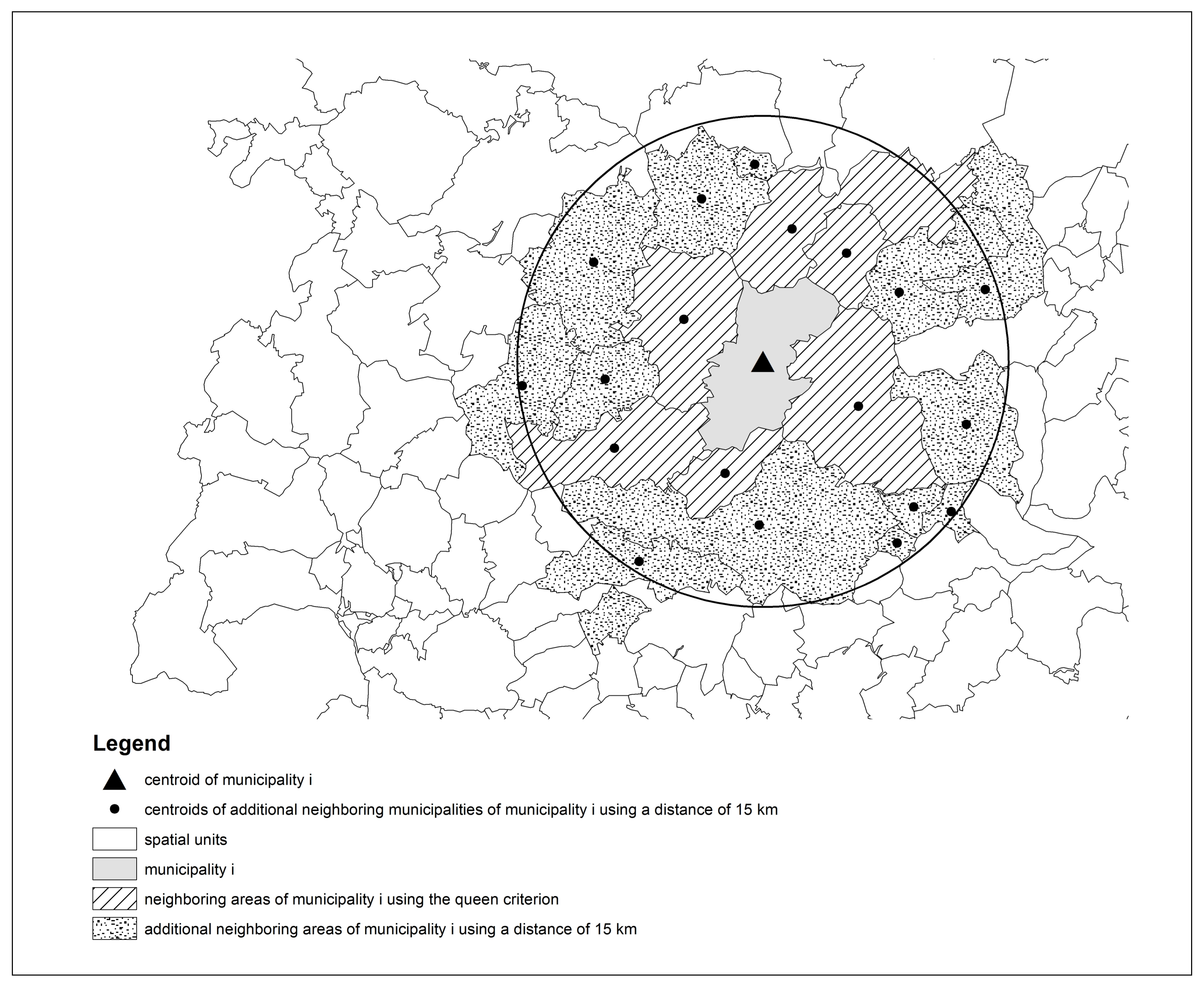
The hedonic pricing model has become the standard empirical approach for modeling agricultural land values as a function of specific attributes [11]. As farmland is a spatially-fixed asset, it is reasonable to take spatial effects into account when empirically estimating the hedonic pricing model for farmland values. Hence, we use a spatial regression model to account for possible spatial dependence and spatial heterogeneity. This ensures unbiased, consistent and efficient estimation results [25]. Spatial neighborhood relationships are integrated by spatial weight matrices, which have to be defined exogenously by the researcher [6,26]. In the first step, a criterion for defining which of the spatial units are neighbors needs to be determined. Figure 1 shows two commonly-used neighborhood criteria, cf. [6,9,27,28].
On the one hand, Figure 1 shows the spatial relationships for municipality i according to a queen contiguity scheme. In analogy with the game of chess, the queen criterion states that municipalities are neighbors for municipality i only if they share a common border or vertex with i on the map [27,30]. This is depicted by the striped spatial units in Figure 1. Hence, municipality i has six neighbors according to the queen criterion. On the other hand, Figure 1 shows the spatial relationships for municipality i according to a distance contiguity scheme. Here, municipalities are neighbors for municipality i only if their centroids are within a specified radius around i. This is depicted by the sum of the striped and speckled spatial units in Figure 1. Hence, municipality i has 19 neighbors in total using a radius of 15 km. If two municipalities are neighbors according to the neighborhood criterion, they receive a relationship in the matrix of one, otherwise zero. The diagonal elements of the matrix are usually set to zero, so municipalities are not considered neighbors to themselves [31].
In a second step, the weights given to each neighbor need to be determined. Common approaches are a binary scheme assigning an equal weight of one to each of all neighbors and a distance scheme weighting geographically closer municipalities more strongly than more distant municipalities [6]. As a rule, the spatial weight matrix is considered in row-standardized form, meaning that each element is divided by its respective row sum, so that each row of the matrix adds up to one [31]. This enables better interpretability of the spatial estimation parameters [25]. For example, using binary weights for the queen contiguity scheme in Figure 1, each of the six neighboring municipalities receives a row-standardized weight of one-sixth for municipality i.
Spatial dependence can occur in the dependent variable as a result of spill-over effects. In the case of farmland, prices in one municipality can be influenced by realized prices in neighboring areas. This effect arises because farmers typically act as competitors for land within a specific radius around their farms and usually use reference prices found in the same region [32]. However, to be able to use a price of a comparable lot as a reference, the reference price must be observable before the respective price formation starts [33]. Hence, we take both the spatial relationship, as well as the time constraint into account when defining a first-order contiguity spatial weight matrix W1. With regard to the spatial dependence, we use the queen criterion (cf. Figure 1). Hence, we assume that the directly bordering municipalities represent the relevant farmland market for a farmer in municipality i and prospective buyers only use reference prices found in their relevant markets. With regard to the time constraint, a farmland value in municipality i is only influenced by the neighboring farmland values, which are observed before the farmland value in municipality i is determined. We use binary weights because our data lack information on the exact location of a transacted plot within a municipality, cf. [6,28]. The matrix is considered in row-standardized form, and the diagonal elements are set to zero. Hence, the spatiotemporally-lagged farmland value (W1y) is treated as an exogenous explanatory variable and can be interpreted as the locally-weighted average farmland value of the adjacent municipalities of previous years.
Spatial heterogeneity refers to variation in relationships over space [30]. For example, spatially- correlated error terms arise if at least one spatially-distributed explanatory variable (e.g., climate factors) is omitted. For the error term, we define a row-standardized binary weighted queen-contiguity spatial weight matrix W2.
Accordingly, our hedonic pricing model using a spatiotemporal regression framework is given by:
where y is an n × 1 vector of farmland values (n = number of observations), W1 is the n × n spatial weight matrix that defines the relevant neighborhood of each observation by simultaneously considering the time constraint and is the respective coefficient for the exogenously-treated spatiotemporally lagged farmland value. X is an n × k matrix of explanatory variables with an associated k × 1 vector of regression coefficients (k = number of explanatory variables). The disturbance term u follows a first-order spatial autoregressive process, where W2 is another n × n spatial weight matrix, is the corresponding spatial autoregressive parameter and is an n × 1 vector of the remaining error term.
Moran’s I tests confirm the existence of spatial autocorrelation in the data and robust Lagrange multiplier tests indicate that both spatial effects have to be considered (for both federal states and all model specifications, the test results are highly significant, p-value < 0.0000). We use the multi-step approach of [34,35], which results in an unbiased and efficient estimation in the presence of spatial effects. Additionally, this estimation method is robust against unknown forms of heteroscedasticity. The procedure consists of two steps alternating a generalized method of moments and two-stage least squares estimators. Due to the lack of acceptable instruments, we have to assume all explanatory variables as exogenous.
5. Data
In this study, we use the standard farmland value (SFV) for arable land and grassland as the dependent variable in the hedonic pricing model. For both federal states, the SFV is determined by regional appraisers at intervals of two years. Data are available for 2008–2012 in Thuringia and for 2007–2013 in Rhineland-Palatinate. The SFV is an average value of nearly all farmland sales within the agricultural sector obtained from data on purchasing prices of the real estate appraiser board of the respective federal state. Only arm’s length transactions are considered. Unfortunately, none of the data on purchasing prices are generally available. Thus, in Germany, the SFV is usually the best available variable for research purposes.
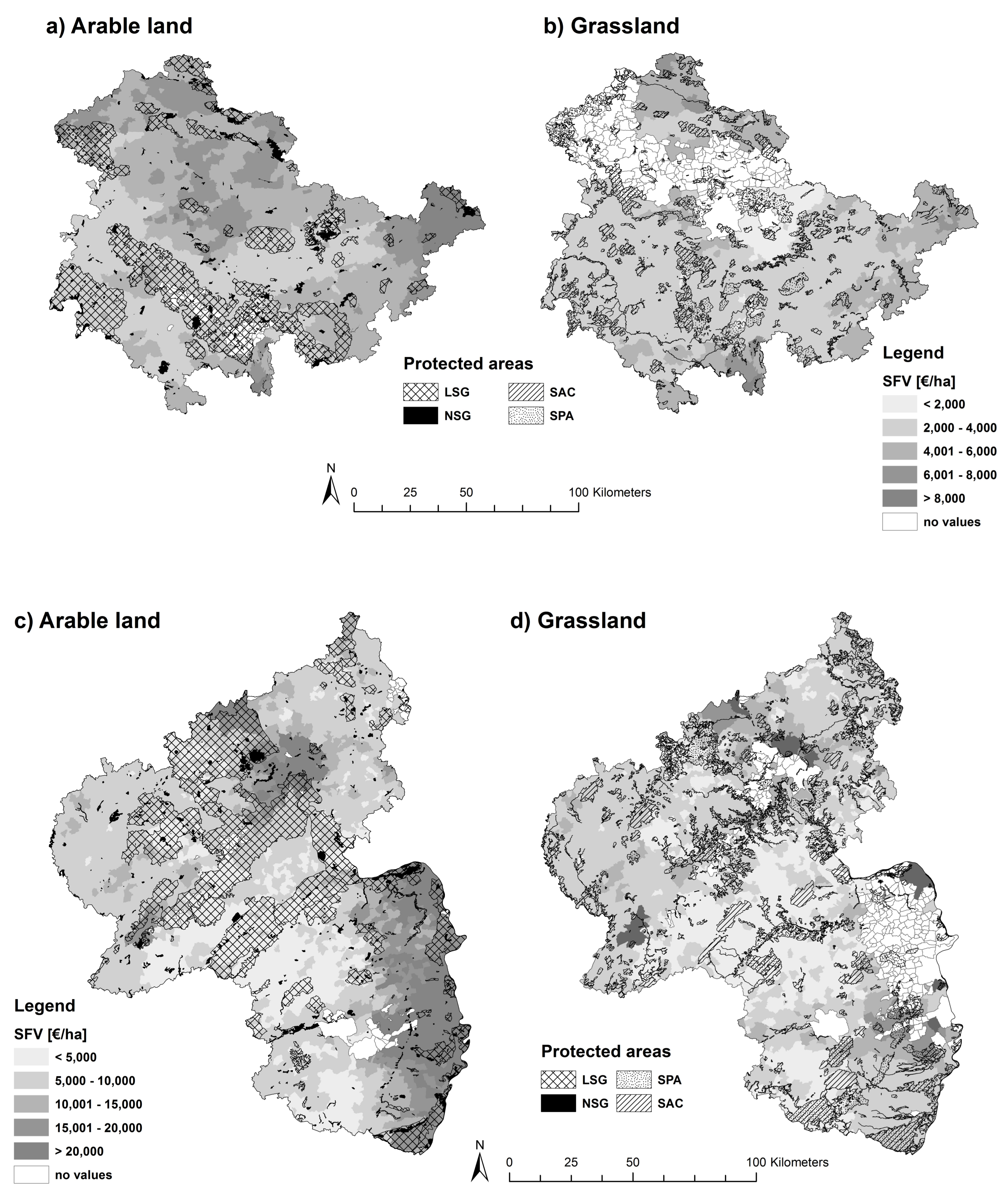
Figure 2 illustrates the spatial distribution of the SFV for arable land and grassland in Thuringia (a and b). The mean SFV for arable land is 5094 Euro/ha in 2012, ranging from 1750–12,500 Euro/ha. The highest values are found in the east and in the north of the federal state, while the central part is characterized by lower SFVs. For grassland, the mean SFV is 3646 Euro/ha with a lower variation ranging from 2000–8455 Euro/ha. High SFVs are found in the peripheral regions of Thuringia.
Parts c and d of Figure 2 show the SFV for arable land and grassland in Rhineland-Palatinate. The mean SFV for arable land amounts to 8959 Euro/ha in 2013 ranging from 3000–51,970 Euro/ha. High values form a cluster in the northern part and a belt in the southeastern edge of the federal state. For grassland, the mean SFV is 6804 Euro/ha varying between 3000 and 41,000 Euro/ha. High SFVs for grassland are scattered across Rhineland-Palatinate.
Furthermore, Figure 2 shows the spatial distribution of the different types of protected areas. For both federal states, the areas of protected landscapes and nature reserves are presented on the left side of the figure. It is obvious that protected landscapes are larger than nature reserves, and both types overlap each other in some regions. On the right side of Figure 2, the Natura 2000 areas are shown. Again, Special Areas of Conservation and Special Protection Areas overlap each other in some regions. Additionally, Figure 2 shows that national protected areas and Natura 2000 areas can also overlap each other.
We estimate separate models for arable land and grassland because the explanatory variables are assumed to affect arable land and grassland differently [15]. Due to the overlapping of the different types of protected areas, we decided to estimate separate models for European (SAC and SPA) and national (NSG and LSG) protected areas.
Table 3 shows the descriptive statistics for the calculation of the spatiotemporally lagged standard farmland value for arable land and grassland in Thuringia and Rhineland-Palatinate. With regard to the time constraint of the spatiotemporally lagged variable, the standard farmland value for a Thuringian municipality in 2012 can only be influenced by standard farmland values of adjacent municipalities of the years 2008 and 2010. Consequently, the results are only based on the years 2010 and 2012, since we cannot calculate a spatiotemporally lagged standard farmland value for the year 2008. The same applies to Rhineland-Palatinate, where the results are only based on the years 2009–2013. In the regression model, we further include one time dummy variable for the year 2012 in Thuringia and two time dummy variables representing the years 2011 and 2013 in Rhineland-Palatinate.
As described above, the row-standardized weights of the spatial weight matrix using a binary weighting scheme are calculated by “1/number of neighbors”. For example, the maximum number of neighbors for a standard farmland value of arable land in Thuringia is 44. Hence, the minimum row-standardized weight for arable land in Thuringia is 1/44 ( 0.0227). Due to significantly smaller municipalities in Rhineland-Palatinate, the maximum number of neighbors is higher compared to Thuringia. However, the average number of neighbors is similar for both federal states.
Table 4 shows the definitions and descriptive statistics for the other explanatory variables used in this study. Maps of different protected areas were obtained from the Thuringian Regional Office for Environment and Geology [36] and the nature conservation administration of Rhineland-Palatinate [37]. By intersecting each map with the map of administrative regions from the German Federal Agency for Cartography and Geodesy [29], the share of the respective type of protected area per municipality was calculated.
The ability of farmland to generate returns from agricultural production depends on the soil characteristics such as quality and slope. The soil quality index was mostly available from the dataset of the SFVs. Missing values were provided by the responsible tax offices. The average slope of agricultural land was generated based on altitudes given by the digital terrain model of the Federal Agency for Cartography and Geodesy [38] and a land use map of the German Federal Institute for Geosciences and Natural Resources [39]. The extraction of agricultural land by using the land use map resulted in some missing values. For these municipalities, we used the average slope of total area as an approximation.
Government payment programs are a further source of income and, thus, could be capitalized into farmland prices. Payments for agro-environmental measures were obtained from the published information on recipients of EU direct payments for the year 2013 [40]. The level of direct payments for farmers of the CAP is equal within the federal states, and only minor differences exist between them. Thus, these payments were not included in the analysis. The Renewable Energies Law can lead to higher competition for land from the cultivation of energy crops. Data on biogas plants are published by the transmission system operators 50 Hertz Transmission and Amprion. The location of the respective plant operator was used as an approximation for the site of the plant.
All other variables are provided by the Federal Statistical Offices of Thuringia and Rhineland-Palatinate [41,42], except for data on income, which are provided by the German Federal Statistical Office [43]. The number of farms and farm sizes reflect the local competition between farmers for agricultural land. Population density, population change and income are variables to capture the impacts of non-agricultural land use. Since non-agricultural land use becomes more likely in proximity to urban centers, we also include the distances to cities with at least 100,000 inhabitants (criterion for large cities). The distance was measured from the centroid of the municipality to the centroid of the city. The fastest road distances to all of the large cities were calculated, and for each municipality, the shortest distance was selected.
6. Results
The estimation results for the SFVs of arable land and grassland for both federal states are given in Table 5. For each federal state and for each type of land use, the first model specification includes the share of LSG and NSG; the second model specification includes the share of SAC and SPA.
The regression coefficient for the spatiotemporally lagged SFV is highly significant in all model specifications. The positive sign of the estimation parameter with a coefficient of approximately 1.15 in Thuringia and 0.91 in Rhineland-Palatinate for arable land indicates that an increase in the spatiotemporally lagged average neighboring SFV by one Euro per hectare raises the SFV in the respective municipality by 1.15 and 0.91 Euro/ha, respectively. Accordingly, the influence of neighboring municipalities is similar in both federal states. However, a coefficient greater than one for Thuringia indicates that the price dynamics are higher in the eastern federal state. Due to a lower initial level, the relative price increases were considerably high during the considered period, resulting in such a high spatiotemporal lag coefficient for arable land. With a coefficient for grassland of approximately 0.97 and 0.89 in Thuringia and Rhineland-Palatinate, respectively, the influence of neighboring municipalities is comparable to the results of arable land.
The spatial autocorrelation parameter (spatial error coefficient) is also significant in all model specifications.
For Thuringia, we find no significant impact of the different shares of protected areas on the SFV for arable land. In contrast, the share of NSG shows a significant price-increasing effect for grassland. An increase by 10% causes the SFV for grassland to raise by 75 Euro/ha. For Rhineland-Palatinate, the effects of the different types of protected areas are more diverse. Here, the shares of LSG and NSG negatively affect the SFV for arable land. The significant price-decreasing effect is (nine-times) higher for the share of NSG. This is a reasonable result as related usage restrictions are higher for NSG compared to LSG (see Table 2). However, both coefficients and the significance level are relatively low. An increase of 10% in the share of LSG or NSG results in a decrease of the SFV for arable land by 13 Euro/ha and 120 Euro/ha, respectively. The share of SPA has a significant and positive correlation with the SFV for arable land. Again, the coefficient and the significance level are relatively low. An increase of 10% in the share of SPA results in an increase of the SFV for arable land by 26 Euro/ha. For grassland, the shares of LSG and SAC have no significant impact on the SFV. In contrast, the shares of NSG and SPA show significant price-increasing effects. An increase of NSG or SPA by 10% causes the SFV for grassland to raise by 118 Euro/ha or 28 Euro/ha. These positive impacts might indicate that grassland utilization is encouraged by protected areas. This can occur if yields of grassland are not considerably negatively affected by usage restrictions related to NSG and SPA, while farmers are sufficiently compensated for higher production costs, e.g., by the contractual nature conservation. Then, grassland utilization might even become economically viable for farmers at first. However, these considerations only apply to the assumption that SFVs for grassland are not strongly influenced by non-agricultural land use purposes. Anyway, a positive correlation at least indicates that related usage restrictions can be more easily fulfilled by grassland utilization compared to arable land.
The remaining explanatory variables only slightly differ between the respective model specifications for the respective type of land use in both federal states. Soil characteristics show the expected effects [11,27]. An increase of one soil point causes the SFV to increase by approximately 27 Euro/ha for arable land and 13–15 Euro/ha for grassland in both federal states. The slope only influences the SFV for arable land in Rhineland-Palatinate. Here, a one percent increase of slope results in a price-discount of 76 Euro/ha. The insignificance in Thuringia might result from a generally lower average slope compared to Rhineland-Palatinate (see Table 4). Additionally, management of arable land might be more concentrated in plain regions, and thus, higher slopes are not an issue for arable land in Thuringia anyway due to geographic circumstances. This is substantiated by the significant price-decreasing impact of slope on grassland for both federal states.
Farm characteristics reveal an interesting finding: while the number of farms positively affects the SFV for arable land in both federal states indicating higher competition for land when the number of farms increases, the impact of farm size differs. An increase of the farm size results in lower prices in Thuringia, but in higher prices in Rhineland-Palatinate. The opposite signs might be explainable by taking into account the different agricultural structures of these federal states. In Rhineland-Palatinate, the farm size is relatively normally distributed (small, medium and large farms exist) resulting in an average farm size of 53 ha (see Table 4). In this range, an increase of the farm size often results in economies of scale and, thus, in a higher willingness to pay for farmland. In contrast, Thuringia has one of the highest disparity between farm sizes. Here, a high number of very small farms and a low number of very large farms exist. As a result, the average farm size is considerably higher (236 ha/farm) compared to Rhineland-Palatinate. Even though we are not able to indicate whether the small or the big farms in Thuringia pay lower prices due to considering the average farm size per municipality, the negative sign of the farm size variable might indicate that very large farms are able to receive price discounts as a result of market power [45,46]. For grassland, the impacts are similar for Rhineland-Palatinate, while no significant impacts are found in Thuringia.
In Rhineland-Palatinate, we also find a price-increasing impact of biogas production on the SFVs for arable land and grassland. Hence, the results indicate higher competition for land when energy crops are cultivated [9]. Non-agricultural factors play a comparatively minor role. Population density is positively correlated with the SFVs for arable land and grassland in both federal states. The positive relationship shows that competition for land between agricultural production and residential purposes exists [10,47]. The impact of income on the SFVs is negative for both types of land use in Rhineland-Palatinate and for grassland in Thuringia. Good non-agricultural earning opportunities may result in a higher share of part-time farmers. If many of them have good non-agricultural income opportunities, the farmers typically do not strive for an increase in farmland, which results in lower competition for land [28]. Payments for agro-environmental measures have a negative impact on the SFV for grassland in Rhineland-Palatinate. However, the coefficient is quite small. All time dummy variables are strongly positively correlated with the SFVs indicating the general upward trend of farmland prices in Germany during the analyzed period [48].
Overall, the high squared correlation coefficient between the predicted and observed values of the dependent variable (R2) indicates good model fits for all model specifications in both federal states, especially for arable land.
7. Discussion and Conclusions
In Germany, nature conservation is mainly realized by the designation of different types of both national and transnational protected areas. National protected areas have their individual legislative decrees including the related commandments and prohibitions for the (agricultural) land use, but an overview of related usage restrictions for agricultural production is missing. However, related information is crucial for examining the impact of protected areas on farmland values. Hence, this study is a first attempt to fill this gap by giving such an overview for the German federal states Thuringia and Rhineland-Palatinate.
The empirical results indicate that protected areas can influence standard farmland values, but the impact must not always be negative. Hence, our first hypothesis is only partly supported. Furthermore, we find differences with regard to the sign and magnitude of the effect depending on the type of protected area (1), the type of land use (2) and the federal state (3). These findings lend support to our second hypothesis. Hence, the impact of protected areas on standard farmland values needs a differentiated discussion according to these three influencing factors.
(1) The impact of nature conservation depends on the type of protected area. In contrast to all of the other analyzed types, Special Areas of Conservation have no significant impact regardless of land use type and region. Such areas are designated to protect special habitats. As described above, the most relevant habitat for Germany belongs to grassland formations, which may explain the insignificant effect on arable land. The work in [49] analyzed the habitat types listed in the annex of the Habitats Directive and identified 63 habitat types that depend on or which can profit from agricultural management. Most of them depend on grazing and mowing, which illustrates the importance of grassland in Special Areas of Conservation. The work in [50] examined the relationship between agriculture and nature conservation from the opposite perspective, i.e., the effects of agriculture on the landscape habitat diversity in Natura 2000 sites of Greece. They focused on the impacts of arable land and also found some insignificant results, as well as differences with regard to the sign and magnitude of the significant effects on different habitat groups based on non-parametric Spearman’s rank correlation coefficients. Overall, they concluded that agriculture does not have a negative effect on landscape habitat diversity.
Moreover, not the total area, but plots representing one of the habitats (and partly also adjacent parcels) are protected, and a variety of different measures exist, ranging from the maintenance of current land use to rewetting of agricultural land. Hence, related impacts on the value of farmland can considerably differ. This is possibly reflected by the insignificance in the empirical results.
However, as described above, the implementation of the Special Areas of Conservation is a multistage process. While the step of selecting the most suitable areas has been completed in Germany since 2006, there are several areas for which a legally-watertight definition of the favorable conservation status and related nature conservation measures are still missing. As Natura 2000 areas belong to large-scale protected areas, the implementation for the remaining areas could affect large amounts of agricultural land (cf. [51]), and thus, a negative impact of Special Areas of Conservation on farmland values may arise in the future.
(2) The impact of protected areas depends on the type of land use. Protected landscapes and nature reserves negatively influence the standard farmland value for arable land in Rhineland-Palatinate. This indicates that related usage restrictions can reduce the value of farmland. A survey by [16] of credit institutes and agricultural experts substantiates our results. Nine of ten credit institutes expected a negative impact of protected areas on the market and loan value of farmland. Two hundred sixty three agricultural experts estimated the depreciation at a minimum of 15% and a maximum of 88% on average, but clearly stated that nature reserves lead to considerably higher losses of value compared to protected landscapes.
While there is evidence for a negative effect on arable land, grassland is mainly positively influenced by nature reserves and Special Protection Areas. As grassland combines various ecological functions regarding biodiversity, water, soil and climate protection [52], the compatibility of grassland utilization and nature conservation as indicated here is a promising result. Possibly, grassland is less affected, as its use can be more easily combined with nature conservation measures compared to arable land. The main reason for this could be the method of management, which differs between both types of land use. Management of arable land is usually more intensive in terms of pesticides or fertilizer, as well as soil compaction. As the loss of ecological heterogeneity and the loss of wild flora and fauna species dependent on farmland habitats are often associated with agricultural intensification and specialization of land use [50,53], regulations to save biodiversity are likely to be more restrictive for intensively-managed arable land ([53] referred to the abandonment of extensively-farmed habitats as a further reason for the loss of biodiversity).
In this context, [53] further found on the basis of a literature review that organic farming has been proven to be strongly advantageous for biodiversity. They presented a new label “Farming for Biodiversity” introduced with the aim of making nature conservation achievements of organic farms visible to consumers. They applied the underlying whole farm assessment system to 50 organic farms in north-eastern Germany and found a high diversity of arable plant species, even on fields without supplementary nature conservation measures. Furthermore, most of the farms easily achieved the total number of credit points for the large-scale measures required for the nature conservation certificate. Hence, the impact of protected areas on organically-managed farmland could be less pronounced compared to conventional farming.
(3) There are regional differences with respect to the impact of protected areas. While in Thuringia, only nature reserves are significantly and positively correlated with standard farmland values for grassland, the impacts are more differentiated in Rhineland-Palatinate (cf. (1) and (2)). The farmland market is quite different between East and West Germany. In eastern federal states, regional farmland markets are more dynamic, resulting in a higher share or farmland sold per year. Furthermore, the average amount of hectares sold per transaction is considerably higher in the eastern federal states [48]. Such land transactions mostly include several parcels, and a total price for the whole area is arranged. Hence, price discounts may be made only rarely for included protected plots in Thuringia.
Overall, the relatively low significance levels and coefficients indicate that farmland values are only slightly affected on average by the usage restrictions related to different types of protected areas.
However, it has to be clearly stated that individual farmers can surely be strongly affected by usage restrictions. According to [54], the designation of a protected area can result in such negative economic and financial consequences for individual farmers that a land use change from purely agricultural purposes to land management under nature conservation measures can endanger their operational existence. This is particularly true if the whole farm is located in a protected area. Such negative effects have to be adequately compensated [51], or the other way round, achievements of the farmers with regard to biodiversity services should be honored, e.g., through agri-environmental schemes or by means of adequate product revenues [53]. According to [55], payments for ecosystem services often face the problem of information asymmetries, which are a key source of inefficiency due to the problems of adverse selection and overcompensation. Using a conceptual agent-based simulation model where payments are either fixed or set through a uniform or discriminatory auction, the authors found that fixed payment schemes can be much more effective than auctions in certain settings. They concluded that relative effectiveness depends on the context (baseline compliance with program standards among the participants, correlation between opportunity costs and ecosystem services in the landscape, heterogeneity in costs and budget size), which should be taken into serious consideration when a payment program design is chosen.
For agricultural policy, the heterogeneity in costs for providing biodiversity services among the individual farms makes it difficult to set the optimal level of support. For example, [56] used a spatially-explicit choice model to build a supply curve of the traditional and high nature value farming system in southern Portugal and predicted that the proportion of traditional farming increased from 20%–80% of the landscape, when economic incentives increased from about 100–160 Euro/ha. The work in [53] showed costs resulting from the integration of nature conservation measures ranging from 27 to more than 1000 Euro/ha depending on the farming system (e.g., dairy or suckler cows), site conditions (e.g., soil quality) and farming intensity.
For farmers, another problem is that the financing of nature conservation is often not ensured in the long run. For example, in both analyzed German federal states, the terms of contractual nature conservation and other support programs usually last five years. For the subsequent funding period, eligible activities can be newly developed or support payments can be changed. Related uncertainty for farmers should be eliminated, e.g., by an increase of financial funding resources, a (more) continuous CAP and by including farmers in the development or adjustments of protection measures. The work in [57] conducted semi-structured, open-ended interviews with farmers and officials to target the effects of the CAP tree density limit on the management of biodiversity-rich wood pastures in southern Sweden. The study revealed, on the one hand, many difficulties in managing the complex relations within landscapes with simplified legal measures, and on the other hand, a general critique concerned the endless and swiftly introduced changes within the CAP that do not harmonize with biophysical cycles guiding agricultural practices. Farmers and officials mentioned that it is this kind of swift change in policy that put constraints on their relationship and trust.
The need to increase funding of nature conservation by farmers becomes also obvious, when considering that habitats dependent on agricultural practices had a worse conservation status than non-agricultural habitats [49].
It would be possible to transfer a higher share of support payments from the first to the second pillar of the CAP and using the extra money for compensation payments related to nature conservation. A reallocation of payments is already claimed by several stakeholders to achieve the concept of “public money for public services” [58]. Using extra money for nature conservation would definitely fit in this concept. It is further possible to grant a top-up premium in the framework of the direct payments of the first pillar of the CAP to farms cultivating farmland located in protected areas, cf. [56]. This top-up can be adjusted to the level of protection. However, these payments of the CAP are also not guaranteed in the long run. Hence, any financing approach for nature conservation that rests on payments of the CAP implies uncertainty for both farmers and nature conservation authorities.
There might be two alternative financing models. First, the regulation of intervention in nature according to § 14 (1) BNatSchG could be expanded by providing the long-term cultivation of protected agricultural land as an alternative compensation measure. The perpetrator of the intervention in nature can monetarily compensate environmental damage by paying the farmer to cultivate protected land. Such payments and related cultivation of protected land can be contractually guaranteed in the long run. However, this approach can only support the financing of nature conservation as it cannot guarantee that all agricultural land located in protected areas can be cultivated by the means of these contracts.
Second, previous studies found that natural amenities are also an important factor affecting farmland values. For example, [1] included the distance to protected federal land as an indicator for natural amenities in a hedonic agricultural land value model, whereby proximity had a significant price-increasing impact. Further studies analyzed such spillover effects of natural amenities on farmland values. A positive relationship was found for indicators like view diversity due to nearby wildlife habitats and amount of fish habitats [13], wildlife recreation (hunting, fishing, wildlife watching) [59], proximity to open space amenities [11,15], as well as the share of wetland and conservation land of the surrounding area [60]. All studies concluded that residents have a higher willingness to pay for living places providing natural amenities. As the protected areas are able to provide natural amenities like open space and recreation opportunities, resulting premium payments of residents could be used to compensate farmers for related losses of agricultural revenues. This opportunity of interpersonal compensation can lead to a welfare improvement following the Kaldor–Hicks-criterion [61]. The high willingness to pay of residents for natural amenities could also be used for compensating losses of returns from non-agricultural sources due to the prohibition of conversion to building land in most of the protected areas.
However, the aggregation level of data should also be taken into account. The standard farmland value is an average value for each municipality. On the one hand, the effect of lower single prices for farmland affected by protected areas might get lost by averaging all sale prices. On the other hand, the designation of conservation areas could also result in an increase of competition for remaining unprotected agricultural land. Due to the aggregation level, this price-increasing impact might compensate negative effects to a certain level. Given that the net effect of protected areas in our analysis is often insignificant, this could reflect the heterogeneity in this relationship. Hence, for further analyses of potential competition between agricultural production and nature conservation, a lower aggregation level of data could be useful, e.g., single sale prices with the information if the respective plot is located in a protected area. The regional appraisers could conduct analyses by means of the spatial regression method developed in this study at a small-scale level, as they have not only the exact location of the individual plot, but also the individual data of farmland prices that are not available to science due to data protection. Such small-scale regional studies may be able to take advantage of less aggregated data to elucidate the impact of protected areas on farmland values, both from the perspective of a direct negative impact on the production intensity of protected farmland and from the perspective of an indirect positive impact of increased competition for remaining unprotected farmland. Improved estimation of impacts of protected areas on agricultural land values is in any case vital for policies aiming at a future conflict-free combination of agricultural production and open space preservation.
Acknowledgments
This work was supported by the H. Wilhelm Schaumann Foundation, Hamburg, Germany.
Author Contributions
Friederike Lehn and Enno Bahrs conceived of and designed the study. Friederike Lehn collected and analyzed the data. Friederike Lehn and Enno Bahrs wrote the paper.
Conflicts of Interest
The authors declare no conflict of interest.
Abbreviations
The following abbreviations are used in this manuscript:
| BNatSchG | Federal Act for the Protection of Nature |
| CAP | Common Agricultural Policy |
| EU | European Union |
| LSG | protected landscapes |
| NSG | nature reserves |
| RLP | Rhineland-Palatinate |
| SAC | Special Areas of Conservation |
| SFV | standard farmland value |
| SPA | Special Protection Areas |
| TH | Thuringia |
References
- Wasson, J.R.; McLeod, D.M.; Bastian, C.T.; Rashford, B.S. The effects of environmental amenities on agricultural land values. Land Econ. 2013, 89, 466–478. [Google Scholar] [CrossRef]
- Lancaster, K.J. A new approach to consumer theory. J. Political Econ. 1966, 74, 132–157. [Google Scholar] [CrossRef]
- Rosen, S. Hedonic prices and implicit markets: Product differentiation in pure competition. J. Political Econ. 1974, 82, 34–55. [Google Scholar] [CrossRef]
- Breustedt, G.; Habermann, H. The incidence of EU per-hectare payments on farmland rental rates: A spatial econometric analysis of German farm-level data. J. Agric. Econ. 2011, 62, 225–243. [Google Scholar] [CrossRef]
- Kilian, S.; Antón, J.; Salhofer, K.; Röder, N. Impacts of 2003 CAP reform on land rental prices and capitalization. Land Use Policy 2012, 29, 789–797. [Google Scholar] [CrossRef]
- Feichtinger, P.; Salhofer, K. The Fischler reform of the common agricultural policy and agricultural land prices. Land Econ. 2016, 92, 411–432. [Google Scholar] [CrossRef]
- Lence, S.H.; Mishra, A.K. The impacts of different farm programs on cash rents. Am. J. Agric. Econ. 2003, 85, 753–761. [Google Scholar] [CrossRef]
- Mishra, A.K.; Moss, C.B. Modeling the effect of off-farm income on farmland values: A quantile regression approach. Econ. Model. 2013, 32, 361–368. [Google Scholar] [CrossRef]
- Hennig, S.; Latacz-Lohmann, U. The incidence of biogas feed-in tariffs on farmland rental rates—Evidence from northern Germany. Eur. Rev. Agric. Econ. 2016, 44, 1–24. [Google Scholar] [CrossRef]
- Livanis, G.; Moss, C.B.; Breneman, V.E.; Nehring, R.F. Urban sprawl and farmland prices. Am. J. Agric. Econ. 2006, 88, 915–929. [Google Scholar] [CrossRef]
- Delbecq, B.A.; Kuethe, T.H.; Borchers, A.M. Identifying the extent of the urban fringe and Its impact on agricultural land values. Land Econ. 2014, 90, 587–600. [Google Scholar] [CrossRef]
- Eagle, A.J.; Eagle, D.E.; Stobbe, T.E.; van Kooten, G.C. Farmland protection and agricultural land values at the urban-rural fringe: British Columbia’s agricultural land reserve. Am. J. Agric. Econ. 2014, 97, 282–298. [Google Scholar] [CrossRef]
- Bastian, C.T.; McLeod, D.M.; Germino, M.J.; Reiners, W.A.; Blasko, B.J. Environmental amenities and agricultural land values: A hedonic model using geographic information systems data. Ecol. Econ. 2002, 40, 337–349. [Google Scholar] [CrossRef]
- Uematsu, H.; Khanal, A.R.; Mishra, A.K. The impact of natural amenity on farmland values: A quantile regression approach. Land Use Policy 2013, 33, 151–160. [Google Scholar] [CrossRef]
- Borchers, A.; Ifft, J.; Kuethe, T. Linking the price of agricultural land to use values and amenities. Am. J. Agric. Econ. 2014, 96, 1307–1320. [Google Scholar] [CrossRef]
- Mährlein, A.; Jaborg, G. Wertminderung landwirtschaftlicher Nutzflächen durch Naturschutzmaßnahmen. Agrarbetrieb 2015, 3, 60–64. [Google Scholar]
- Bundesamt für Naturschutz. Daten zur Natur 2016: Bundesamt für Naturschutz; Görres-Druckerei und Verlag GmbH: Neuwied, Germany, 2016. [Google Scholar]
- EC. Natura 2000. 2009. Available online: http://ec.europa.eu/environment/nature/info/pubs/docs/nat2000/factsheet_en.pdf (accessed on 28 June 2017).
- Bundesamt für Naturschutz. Protected Areas and Natura 2000: Federal Agency for Nature Conservation. 2017. Available online: https://www.bfn.de/en/activities.html (accessed on 14 February 2018).
- LANIS. Die Landschaftsschutzgebiete in Rheinland-Pfalz: Landscape Information System of the Nature Conservation Administration in Rhineland-Palatinate. 2017. Available online: https://www.naturschutz.rlp.de/extensions_lanis/extensions/lanis/dyn_lsg.php (accessed on 14 September 2017).
- LANIS. Die Naturschutzgebiete in Rheinland-Pfalz: Landscape Information System of the Nature Conservation Administration in Rhineland-Palatinate. 2017. Available online: http://www.naturschutz.rlp.de/extensions_lanis/extensions/lanis/dyn_nsg.php (accessed on 14 September 2017).
- Thüringer Staatsanzeiger. Legislative Decrees of Nature Reserves and Protected Landscapes in Thuringia: Gisela Husemann Verlag. 2018. Available online: http://stanzon.husemann.net/index.php (accessed on 16 January 2018).
- LANIS. Endgültige Bewirtschaftungspläne: Landscape Information System of the Nature Conservation Administration in Rhineland-Palatinate. 2017. Available online: http://www.naturschutz.rlp.de/?q=bewirtschaftungsplaene (accessed on 19 October 2017).
- TLUG. Liste der Pflegeempfehlungen für Hochwertige Biotoptypen: Thuringian Regional Office for Environment and Geology. 2017. Available online: https://www.thueringen.de/imperia/md/content/tlug/abt3/natura2000/pflege_c1_lebensraum.pdf (accessed on 19 October 2017).
- Anselin, L. Spatial Econometrics: Methods and Models; Kluwer Academic Publishers: Dordrecht, The Netherlands; Boston, MA, USA; London, UK, 1988. [Google Scholar]
- Bivand, R.S.; Pebesma, E.; Gómez-Rubio, V. Applied Spatial Data Analysis with R, 2nd ed.; Springer Verlag: New York, NY, USA, 2013. [Google Scholar]
- Huang, H.; Miller, G.Y.; Sherrick, B.J.; Gómez, M.I. Factors influencing Illinois farmland values. Am. J. Agric. Econ. 2006, 88, 458–470. [Google Scholar] [CrossRef]
- Hüttel, S.; Odening, M.; Kataria, K.; Balmann, A. Price formation on land market auctions in East Germany—An empirical analysis. Germ. J. Agric. Econ. 2013, 62, 99–115. [Google Scholar]
- GEOBASIS-DE/BKG. Verwaltungsgebiete der Bundesrepublik Deutschland. Anwendungsmaßstab 1: 250.000: Stand 01.01.2011; Federal Agency for Cartography and Geodesy: Frankfurt am Main, Germany, 2015. [Google Scholar]
- LeSage, J. Spatial Econometrics. 1998. Available online: http://www.spatial-econometrics.com/html/wbook.pdf (accessed on 1 November 2017).
- LeSage, J.; Pace, R.K. Introduction to Spatial Econometrics; Taylor & Francis Group: Boca Raton, FL, USA, 2009. [Google Scholar]
- Maddison, D. A Spatio-temporal model of farmland values. J. Agric. Econ. 2009, 60, 171–189. [Google Scholar] [CrossRef]
- Hüttel, S.; Wildermann, L. Price formation in agricultural land markets—How do different acquiring parties and sellers matter? In Neuere Theorien und Methoden in den Wirtschafts- und Sozialwissenschaften des Landbaus. Schriften der Gesellschaft für Wirtschafts- und Sozialwissenschaften des Landbaus; Landwirtschaftsverlag: Münster, Germany, 2015; Volume 50, pp. 125–142. [Google Scholar]
- Kelejian, H.H.; Prucha, I.R. HAC estimation in a spatial framework. J. Econ. 2007, 140, 131–154. [Google Scholar] [CrossRef]
- Kelejian, H.H.; Prucha, I.R. Specification and estimation of spatial autoregressive models with autoregressive and heteroskedastic disturbances. J. Econ. 2010, 157, 53–67. [Google Scholar] [CrossRef] [PubMed]
- TLUG. Internet Presence: Thuringian Regional Office for Environment and Geology. 2015. Available online: http://www.tlug-jena.de/kartendienste/ (accessed on 26 July 2017).
- LANIS. Landscape Information System. 2015. Available online: http://map1.naturschutz.rlp.de/kartendienste_naturschutz/index.php (accessed on 28 July 2017).
- GEOBASIS-DE/BKG. Digitales Geländemodell. Gitterweite 200 m. DGM 200.; Federal Agency for Cartography and Geodesy: Frankfurt am Main, Germany, 2015. [Google Scholar]
- BGR. Nutzungsdifferenzierte Bodenübersichtskarte der Bundesrepublik Deutschland 1:1.000.000 (BÜK 1000 N2.3); Federal Institute for Geosciences and Natural Resources: Hannover, Germany, 2015. [Google Scholar]
- BLE. Zahlungen aus den Europäischen Fonds für Landwirtschaft und Fischerei; Federal Office for Agriculture and Food: Bonn-Mehlem, Germany, 2015. [Google Scholar]
- Federal Statistical Office Thuringia. Landesdatenbank. 2017. Available online: http://www.tls.thueringen.de/ (accessed on 26 July 2017).
- Federal Statistical Office Rhineland-Palatinate. Landesdatenbank. 2017. Available online: http://www.statistik.rlp.de/de/startseite/ (accessed on 28 July 2017).
- Destatis. The Regional Database Germany: German Federal Statistical Office. 2017. Available online: https://www.regionalstatistik.de/genesis/online/logon (accessed on 20 November 2015).
- Piras, G. sphet: Spatial Models with Heteroskedastic Innovations in R. J. Stat. Softw. 2010, 35. [Google Scholar] [CrossRef]
- Balmann, A. Braucht der ostdeutsche Bodenmarkt eine stärkere Regulierung? Spec. Suppl. AgraEur. 2015, 13/15, 1–7. [Google Scholar]
- Back, H.; Menzel, F.; Bahrs, E. Konzentrationsmessung der Bewirtschaftung landwirtschaftlicher Flächen zur Schätzung der Marktmacht auf den deutschen Bodenmärkten. Jahrbuch der Österreichischen Gesellschaft für Agrarökonomie 2016, 25, 191–200. [Google Scholar]
- Cavailhès, J.; Thomas, I. Are agricultural and developable land prices governed by the same spatial rules? The case of Belgium. Can. J. Agric. Econ. 2013, 61, 439–463. [Google Scholar] [CrossRef]
- Destatis. Land- und Forstwirtschaft, Fischerei. Kaufwerte für landwirtschaftliche Grundstücke; 2016: Fachserie 3, Reihe 2.4; Statistisches Bundesamt: Wiesbaden, Germany, 2017.
- Halada, L.; Evans, D.; Romao, C.; Petersen, J.E. Which habitats of European importance depend on agricultural practices? Biodivers. Conserv. 2011, 20, 2365–2378. [Google Scholar] [CrossRef]
- Kallimanis, A.S.; Tsiafouli, M.A.; Pantis, J.D.; Mazaris, A.D.; Matsinos, Y.; Sgardelis, S.P. Arable land and habitat diversity in Natura 2000 sites in Greece. J. Biol. Res. Thessalon. 2008, 9, 55–66. [Google Scholar]
- Mährlein, A. Inanspruchnahme landwirtschaftlicher Flächen durch Naturschutzmaßnahmen: Ökonomische Bewertung der Verluste an Fläche, Einkommen, Vermögen und Beleihungswert. Agrarbetrieb 2017, 5, 370–380. [Google Scholar]
- Nitsch, H.; Osterburg, B.; Roggendorf, W.; Laggner, B. Cross compliance and the protection of grassland—Illustrative analyses of land use transitions between permanent grassland and arable land in German regions. Land Use Policy 2012, 29, 440–448. [Google Scholar] [CrossRef]
- Gottwald, F.; Stein-Bachinger, K. ‘Farming for Biodiversity’—A new model for integrating nature conservation achievements on organic farms in north-eastern Germany. Org. Agric. 2018, 8, 79–86. [Google Scholar] [CrossRef]
- Mährlein, A. Existenzgefährdung landwirtschaftlicher Betriebe infolge öffentlicher Eingriffe: Praktische Handlungsempfehlungen für die Gutachtenerstellung. Agrarbetrieb 2015, 1, 52–58. [Google Scholar]
- Lundberg, L.; Persson, U.M.; Alpizar, F.; Lindgren, K. Context matters: Exploring the cost-effectiveness of fixed payments and procurement auctions for PES. Ecol. Econ. 2018, 146, 347–358. [Google Scholar] [CrossRef]
- Ribeiro, P.F.; Nunes, L.C.; Beja, P.; Reino, L.; Santana, J.; Moreira, F.; Santos, J.L. A spatially explicit choice model to assess the impact of conservation policy on high nature value farming systems. Ecol. Econ. 2018, 145, 331–338. [Google Scholar] [CrossRef]
- Sandberg, M.; Jakobsson, S. Trees are all around us: Farmers’ management of wood pastures in the light of a controversial policy. J. Environ. Manag. 2018, 212, 228–235. [Google Scholar] [CrossRef] [PubMed]
- Forstner, B.; Deblitz, C.; Kleinhanss, W.; Nieberg, H.; Offermann, F.; Röder, N.; Salamon, P.; Sanders, J.; Weingarten, P. Analyse der Vorschläge der EU-Kommission vom 12. Oktober 2011 zur künftigen Gestaltung der Direktzahlungen im Rahmen der GAP nach 2013: Arbeitsberichte aus der vTI-Agrarökonomie; Johann Heinrich von Thünen-Institut: Braunschweig, Germany, 2012. [Google Scholar]
- Henderson, J.; Moore, S. The capitalization of wildlife recreation income into farmland values. J. Agric. Appl. Econ. 2006, 38, 597–610. [Google Scholar] [CrossRef]
- Ma, S.; Swinton, S.M. Hedonic valuation of farmland using sale prices versus appraised values. Land Econ. 2012, 88, 1–15. [Google Scholar] [CrossRef]
- Frambach, H. Basiswissen Mikroökonomie, 3rd ed.; UTB GmbH: Stuttgart, Germany, 2013. [Google Scholar]
Figure 1.
Spatial relationships depending on the chosen neighborhood criterion. Based on [29].
Figure 1.
Spatial relationships depending on the chosen neighborhood criterion. Based on [29].

Figure 2.
Standard farmland values for arable land and grassland, as well as the protected areas in Thuringia (a,b) and Rhineland-Palatinate (c,d). Based on [29].
Figure 2.
Standard farmland values for arable land and grassland, as well as the protected areas in Thuringia (a,b) and Rhineland-Palatinate (c,d). Based on [29].


Table 1.
Characteristics of the most important protected areas in Germany. Based on [19] and BNatSchG.
Table 1.
Characteristics of the most important protected areas in Germany. Based on [19] and BNatSchG.
| Characteristic | SPA | SAC | National Parks | NSG | LSG |
|---|---|---|---|---|---|
| Level of legislation | International/EU (mandatory implementation in national law) | National/Germany | |||
| Statutory fixation | Birds Directive | Habitats Directive | Federal Act for the Protection of Nature (region-specific differences in State Conservation Acts) | ||
| Protection objective | Conservation of all wildlife birds and their habitats | Conservation of biodiversity (plants/ animals) and habitats | Warranty of undisturbed natural processes, natural history education/research | Conservation of special wildlife species (plants/animals), biotic resource protection | Conservation of general appearance of the landscape, abiotic resource protection |
| Level of protection | High (for protected habitats and species; otherwise, no protection) | High | High | Low | |
| Share of area (%) in 1: | |||||
| Germany | 11.30 | 9.30 | 0.60 | 3.90 | 27.60 |
| Thuringia | 14.30 | 10.00 | 0.46 | 3.00 | 25.90 |
| Rhineland- Palatinate | 12.20 | 12.90 | 0.52 | 2.00 | 27.00 |
Note: 1 Only terrestrial protected area is considered. The shares of the individual types of protected areas cannot be summed, because they partly overlap each other; SPA = Special Protection Areas according to the Birds Directive; SAC = Special Areas of Conservation according to the Habitats Directive; NSG = nature reserves; LSG = protected landscapes.
Table 2.
Possible usage restrictions in nature reserves and protected landscapes in the context of agricultural production and the frequency of their occurrence in the reviewed legislative decrees. Research based on [20,21,22].
| Characteristic | NSG | LSG | ||
|---|---|---|---|---|
| Federal state | RLP | TH | RLP | TH |
| Number of total protected areas | 520 | 273 | 109 | 54 |
| Number of reviewed legislative decrees | 50 | 36 | 10 | 2 |
| Share of total protected area covered by the analysis (%) | 55 | 50 | 76 | 15 |
| Land use restrictions | ||||
| No constructions of buildings, roads, etc. | 50 | 36 | 10 | 2 |
| No extraction of mineral resources | 49 | 35 | 10 | 2 |
| No removal of landscape components (trees, shrubs, hedges, etc.) | 33 | - 1 | 10 | - 1 |
| No conversion of grassland in arable land | 19 | 34 | 2 | 1 |
| No cultivation of fallow land | 3 | 33 | - | - |
| Agricultural input restrictions | ||||
| Limitation or prohibition of manure and mineral fertilizer application | 24 | 36 | - | - |
| Limitation or prohibition of plant protection products application | 29 | 36 | - | - |
| Water regulation restrictions | ||||
| No interventions in the water balance | 23 | 27 | - | - |
| No changes of water bodies and wetlands | 31 | 32 | 10 | 1 |
| Limitation or prohibition of surface water or groundwater use | 24 | 35 | 1 | - |
Note: without any claim of completeness. NSG = nature reserves; LSG = protected landscapes; RLP = Rhineland-Palatinate; TH = Thuringia. 1 The removal of landscape components is generally prohibited by the Thuringian federal nature protection act.
Table 3.
Descriptive statistics for the spatiotemporally lagged standard farmland value for arable land and grassland in Thuringia and Rhineland-Palatinate.
Table 3.
Descriptive statistics for the spatiotemporally lagged standard farmland value for arable land and grassland in Thuringia and Rhineland-Palatinate.
| Thuringia | Rhineland-Palatinate | |||
|---|---|---|---|---|
| Arable Land | Grassland | Arable Land | Grassland | |
| number of neighbors | ||||
| mean | 7.82 | 6.89 | 10.28 | 10.00 |
| minimum | 2 | 1 | 2 | 1 |
| maximum | 44 | 40 | 87 | 90 |
| row-standardized weights of neighbors | ||||
| mean | 0.1279 | 0.1451 | 0.0972 | 0.1000 |
| minimum | 0.0227 | 0.025 | 0.0115 | 0.0111 |
| maximum | 0.5000 | 1 | 0.5000 | 1 |
| spatiotemporally lagged SFV (Euro/ha) | ||||
| mean | 4409 | 3561 | 8109 | 6084 |
| std. dev. | 1109 | 758 | 5265 | 2243 |
| minimum | 2221 | 1873 | 3000 | 2333 |
| maximum | 9318 | 7249 | 44,120 | 23,670 |
Table 4.
Definitions and descriptive statistics for the municipal level variables for Thuringia in 2012 and Rhineland-Palatinate in 2013. UAA, utilized agricultural area; AUM, agro-environmental measures.
Table 4.
Definitions and descriptive statistics for the municipal level variables for Thuringia in 2012 and Rhineland-Palatinate in 2013. UAA, utilized agricultural area; AUM, agro-environmental measures.
| 2*Variable | 2*Definition | TH | RLP |
|---|---|---|---|
| Mean (Std. Dev.) 1 | |||
| Dependent variable | |||
| Na | Number of observations for arable land | 818 | 2251 |
| Ng | Number of observations for grassland | 657 | 2067 |
| Year | Year of observation | 2012 | 2013 |
| SFV [Euro/ha] | Standard farmland value for arable land | 5094 (1882) | 8959 (6066) |
| SFV [Euro/ha] | Standard farmland value for grassland | 3646 (1053) | 6804 (2892) |
| Protected areas | |||
| LSG [%] | Share of protected landscapes to total area | 25.77 (36.79) | 26.60 (39.86) |
| NSG [%] | Share of nature reserves to total area | 2.50 (6.72) | 1.41 (4.87) |
| SAC [%] | Share of Special Areas of Conservation to total area | 8.50 (13.81) | 9.47 (15.45) |
| SPA [%] | Share of Special Protection Areas to total area | 15.31 (24.38) | 9.50 (19.79) |
| Further variables | |||
| Soil quality (a) [0;100] | Average soil quality index for arable land | 43.02 (14.68) | 44.02 (13.78) |
| Soil quality (g) [0;100] | Average soil quality index for grassland | 35.77 (9.62) | 37.93 (6.90) |
| Share of UAA [%] | Share of utilized agricultural area to total area | 60.17 (22.80) | 47.63 (19.52) |
| Slope [%] | Average slope of utilized agricultural area | 5.96 (3.36) | 7.86 (3.94) |
| AUM [Euro/ha] | Payments for agro-environmental measures per hectare utilized agricultural area | 8.17 (36.46) | 28.37 (73.09) |
| Farms [Number] | Number of farms in 2010 | 4.26 (6.70) | 9.13 (14.68) |
| Farm size [ha/farm] | Farm size expressed in hectares utilized agricultural area per farm | 236.10 (225.58) | 53.16 (36.45) |
| Biogas [kWel./ha] | Installed electric power of biogas plants per hectare utilized agricultural area | 0.17 (0.68) | 0.12 (0.63) |
| Population density [inhabitants/km2] | Population density | 92.17 (100.90) | 143.80 (156.98) |
| Population change [%] | Percent change in population from 2000–2012 for TH and from 2000–2013 for RLP | −11.89 (8.14) | −3.21 (10.84) |
| Income [Euro/Inhabitant] | Average income per inhabitant | 11,600 (2407) | 12,380 (5775) |
| Distance [km] | Distance to the nearest large city | 78.61 (337.39) | 52.21 (21.03) |
Note: 1 all variables that are not specifically related to the land use type are expressed as an average for all 849 municipalities in Thuringia (TH) and all available 2281 municipalities in Rhineland-Palatinate (RLP).
Table 5.
Estimation results for the standard farmland values of arable land and grassland in Thuringia and Rhineland-Palatinate.
Table 5.
Estimation results for the standard farmland values of arable land and grassland in Thuringia and Rhineland-Palatinate.
| Variable | Thuringia | Rhineland-Palatinate | ||||||
|---|---|---|---|---|---|---|---|---|
| Arable Land | Grassland | Arable Land | Grassland | |||||
| LSG + NSG | SAC + SPA | LSG + NSG | SAC + SPA | LSG + NSG | SAC + SPA | LSG + NSG | SAC + SPA | |
| Intercept | −1376.9 *** | −1381.5 *** | −182.14 | −117.37 | −230.27 | −336.16 | 96.698 | 28.535 |
| LSG | −0.2307 | - | 0.2720 | - | −1.2848 | - | −0.9284 | - |
| NSG | 2.4203 | - | 7.5344 *** | - | −12.039 | - | 11.8230 * | - |
| SAC | - | −0.3241 | - | 0.7631 | - | −0.7228 | - | 0.1071 |
| SPA | - | −1.0168 | - | −1.0764 | - | 2.6346 | - | 2.7817 |
| Soil quality | 26.789 *** | 26.963 *** | 14.537 *** | 14.524 *** | 26.299 *** | 26.951 *** | 12.829 | 12.957 |
| Share of UAA a | - | - | - | - | −0.2251 | 1.2898 | 0.6860 | 1.3620 |
| Slope | −14.252 | −12.785 | −21.314 ** | −18.302 ** | −75.991 *** | −76.506 *** | −34.334 *** | −34.908 *** |
| AUM | −0.0686 | −0.0865 | 0.0355 | −0.0163 | −0.1258 | −0.1482 | −0.4465 * | −0.4515 ** |
| Farms | 6.2534 ** | 6.3597 ** | 1.5092 | 1.5707 | 19.692 *** | 19.348 *** | 11.899 ** | 11.764 ** |
| Farm size | −0.1752 * | −0.1710 * | −0.0414 | −0.0392 | 2.4964 *** | 2.4877 *** | 1.3416 ** | 1.3405 ** |
| Biogas | −7.2713 | −7.8203 | 6.6562 | 3.4543 | 146.28 *** | 150.31 *** | 112.86 ** | 116.52 ** |
| Population density | 0.4928 *** | 0.4767 *** | 0.3402 ** | 0.3325 ** | 2.5376 *** | 2.6315 *** | 2.2078 *** | 2.2139 *** |
| Population change | −2.3729 | −2.2211 | −1.5420 | −1.1069 | −2.7204 | −2.4831 | −3.1510 | −3.1064 |
| Income | 0.0016 | 0.0014 | −0.0117 ** | −0.0120 ** | −0.0092 | −0.0091 | −0.0150 ** | −0.0147 ** |
| Distance | −0.0221 | −0.0219 | −0.0139 | −0.0125 | −0.9932 | −1.3895 | 0.9279 | 0.6556 |
| Dummy (2011) | - | - | - | - | 192.23 *** | 193.24 *** | 282.37 *** | 282.61 *** |
| Dummy (2012) | 167.78 *** | 167.72 *** | 129.54 *** | 131.12 *** | - | - | - | - |
| Dummy (2013) | - | - | - | - | 676.18 *** | 678.71 *** | 668.25 *** | 668.37 *** |
| Spatiotemporal lag | 1.1453 *** | 1.1474 *** | 0.9720 *** | 0.9612 *** | 0.9071 *** | 0.9006 *** | 0.8872 *** | 0.8893 *** |
| Spatial error | 0.7010 *** | 0.6956 *** | 0.3915 *** | 0.3971 *** | 0.3026 *** | 0.3070 *** | 0.4401 *** | 0.4438 *** |
| R2 b [%] | 84.54 | 84.64 | 77.70 | 77.33 | 91.78 | 91.76 | 72.37 | 72.30 |
Note: , *, **, *** significance at the 10, 5, 1 and 0.1 percent level. R command “spreg” is used for estimation [26,44]. UAA = utilized agricultural area; AUM = agro-environmental measures; LSG = protected landscapes; NSG = nature reserves; SAC = Special Areas of Conservation according to the Habitats Directive; SPA = Special Protection Areas according to the Birds Directive. a Share of UAA that had to be excluded due to multicollinearity problems in Thuringia. b Squared correlation coefficient between the predicted and observed values of the dependent variable.
© 2018 by the authors. Licensee MDPI, Basel, Switzerland. This article is an open access article distributed under the terms and conditions of the Creative Commons Attribution (CC BY) license (http://creativecommons.org/licenses/by/4.0/).
Share and Cite
MDPI and ACS Style
Lehn, F.; Bahrs, E. Land-Use Competition or Compatibility between Nature Conservation and Agriculture? The Impact of Protected Areas on German Standard Farmland Values. Sustainability 2018, 10, 1198. https://doi.org/10.3390/su10041198
AMA Style
Lehn F, Bahrs E. Land-Use Competition or Compatibility between Nature Conservation and Agriculture? The Impact of Protected Areas on German Standard Farmland Values. Sustainability. 2018; 10(4):1198. https://doi.org/10.3390/su10041198
Chicago/Turabian StyleLehn, Friederike, and Enno Bahrs. 2018. "Land-Use Competition or Compatibility between Nature Conservation and Agriculture? The Impact of Protected Areas on German Standard Farmland Values" Sustainability 10, no. 4: 1198. https://doi.org/10.3390/su10041198
Note that from the first issue of 2016, this journal uses article numbers instead of page numbers. See further details here.