A Numerical Study of the Temperature Reduction by Water Spray Systems within Urban Street Canyons


Department of Bioenvironmental Systems Engineering, National Taiwan University, Taipei 10617, Taiwan
*
Author to whom correspondence should be addressed.
Sustainability 2018, 10(4), 1190; https://doi.org/10.3390/su10041190
Submission received: 24 February 2018
/
Revised: 10 April 2018
/
Accepted: 11 April 2018
/
Published: 15 April 2018
(This article belongs to the Special Issue Sustainable Energy Development under Climate Change)
Abstract
:To reduce energy demand (both fossil fuel and renewable energy) for cooling the urban heat island environment, some solutions have been studied. Among these methods, the water spray system is considered more flexible due to its dynamic controls. This study investigated the cooling effect of water spray systems in the street canyon under different aspect ratios and high relative humidity environments using a computational fluid dynamics model. This model was validated with water channel and wind tunnel experiments. The results showed that the most effective cooling area was the area just under the spray nozzles. However, in a narrow street canyon, people in the middle of the street may feel the cooling effect because of the dispersion and accumulation of the cooled air. Our simulations demonstrated that air under the nozzles was saturated and this revealed that under drier conditions the water spray systems will have higher cooling performance. We also found that using large water droplets created a wider cooling area in the middle of the street canyon, and this phenomenon was not changed much if the nozzle height was increased from 2.5 m to 3.5 m.
1. Introduction
The urban heat island forms as a result of urbanization and energy consumption (both fossil fuel and renewable energy). It affects urban micrometeorology [1] and aggravates climate change, which has increased the frequency and intensity of heat waves [2], and will then rapidly increase energy demand by 70% for air conditioning during the whole 2000–2100 period [3].
Some adaptations have been confirmed as valid for cooling urban areas or buildings, such as green walls, green ponds [4], roof ponds [5], vegetation, increase of short wave reflectivity, and water spray systems. Among these, the water spray system is considered more flexible with its dynamic controls in warm seasons while passive cooling systems such as vegetation and increase in short wave reflectivity also reduce temperature in all seasons. The water spray system is also an energy efficient, economical, and environmentally friendly method for improving thermal comfort in urban environments [6,7]. Reducing energy consumption for thermal comfort can then lead mitigate climate change (and urban heat island) and form a positive feedback loop for energy demand, climate change, and heat waves relations.
Furthermore, experiments conducted by Jain and Rao (1974) [8] showed that roof water spray systems performed better in reducing ceiling temperature than roof ponds did (15 °C and 13 °C, respectively). Huang et al., (2011) [9] conducted several experiments and proved that the water spray system is very effective since it reduced temperature by 5–7 °C under an ambient temperature of 35 °C and a relative humidity of 45%. In spite of these benefits and universal applications, studies on the cooling effect of water spray systems in urban environments are found to be relatively rare.
Numerical simulation by a Computational Fluid Dynamics (CFD) model is a tool suitable for studying momentum, energy, and particle flows since it is more efficient and cheaper than full-scale measurements and wind-tunnel experiments. However, the interaction between water droplets and air is rather complicated since it is a two-phase flow, which takes into account the effect of energy exchange when droplets evaporate, as well as momentum exchange between droplets and air flow. In order to simulate these effects, the Lagrangian-Eulerian model separates a two-phase flow into the discrete phase part (Lagrangian model) and continuous phase part (Eulerian model), and these two models are coupled during the simulation. Several validation studies with small-scale and full-scale experimental data showed that the Lagrangian-Eulerian model is reliable for simulating the two-phase flow [6,10].
Although the Lagrangian-Eulerian model is widely used to simulate the two-phase flow, there are only a few studies applying this model to urban environments. Montazeri et al., (2017) [7] simulated a water spray system in an urban landscape using the Lagrangian-Eulerian approach. The results showed that for a water spray system installed at a height of 3 m with a water mass flow rate of 0.15 kg/s and under relative humidity of around 30%, a temperature reduction of approximately 7 °C was found at the height of 1.75 m in the courtyard, and thus heat stress was alleviated efficiently. However, the study only simulated the cooling effect in a specific courtyard with fixed meteorological conditions. With different building geometry or meteorological conditions (e.g., relative humidity), the cooling effect may be quite different.
An urban street canyon is the space between buildings that line up continuously along both sides of a relatively narrow urban street. The wind velocity field [11] and pollutants dispersion [12] in urban street canyons have been studied. They concluded that the aspect ratio (building height divided by street width) is a crucial parameter that affects the velocity field and the dispersion of pollutants in the street canyon, in which more pollutants would be trapped in a street canyon with a higher aspect ratio. This phenomenon is likely to influence the outcome of the cooling effect within street canyons, since the cooling effect is affected by the dispersion of water droplets. The water spray system is widely used to reduce air temperature in the urban canyons in residential–commercial mixed areas and night markets in South Asian cities (e.g., Taipei) during summers. Moreover, most of the residential-commercial mixed areas and night markets in Taipei are built in street canyons with aspect ratios larger than 1, which means that the wind velocity would be small in this region. With a high population density, low wind speed, and high temperature in the summer, there is a high demand for using the water spray system to reduce temperatures in the street canyons. However, this cooling effect has not yet been studied in a numerical manner. In order to contribute a wider application of the water spray system, this study applied the Lagrangian-Eulerian model to simulate the cooling effect of water spray systems in the urban street canyon with manipulation of four variables: (1) the aspect ratio of the street canyon; (2) the relative humidity; (3) water droplet size; and (4) the height of the spray nozzle.
2. Methods
2.1. Computational Geometry and Grids
The computational geometry was a 3D long street canyon with building height, H; street width, W; and street length, L; where L was set to be much larger than H. Three types of street canyon, with the aspect ratio H/W = 1, 2, and 3, respectively, were considered in this study (Figure 1); these aspect ratios (H/W) mimic the general street canyons of residential–commercial mixed areas in Taipei city, Taiwan. As shown in Figure 1, the vertical (z direction) computational domain size was two times that of the building height; the building width was the same as the building height. Following Baik and Kim (1999) [11], the horizontal (x direction) domain size was equal to two times that of the building width plus the street width. The street widths (W) were 15, 10, and 5 m for H/W = 1, 2, and 3, respectively. The street lengths (L) were all fixed to be 150 m for the three street canyons.
In terms of meshing the computational domains, uneven grid sizes were adopted; the grids inside the street canyon were set to be finer than those on the outside; the grid size of cells adjacent to the buildings and street were also set to be finer to model the effect of building boundaries. The grid sizes and numbers for the three street canyons were determined with the convergence test on the horizontal velocity. Based on the tests, the number of grids were 295,075, 241,100, and 305,350 for H/W = 1, 2, and 3, respectively. The results of meshing for these three street canyons were shown in Figure 2.
2.2. Numerical Scheme
All of the calculations were performed with ANSYS FLUENT [13]. The Eulerian part of the Lagrangian-Eulerian model contains continuous phases such as flow velocity field, temperature field, and vapor concentration field. These were solved with 3D Reynolds-Averaged Navier-Stokes equations combined with the energy equation (see Appendix A). Closure was obtained by the Re-Normalization Group (RNG) k-ε model. The model validation by Chan et al., (2002) [12] suggested the RNG k-ε model is an optimum model (compared to the standard k-ε model) and a realizable model when simulating the flow field in a street canyon. In this study, pressure–velocity coupling was performed with the Semi-Implicit Method for Pressure Linked Equations (SIMPLE). Second-order discretization schemes were used for all convection and viscous terms and second-order implicit time integration was used for the temporal discretization. Note that second-order implicit time integration could avoid the sharp temperature reduction caused by the accumulation of droplets when a large velocity gradient occurs.
The Lagrangian part of the Lagrangian-Eulerian model, including discrete phases such as velocity, temperature, and mass of water droplets (see Appendix B) were solved with the discrete phase model (DPM) implemented by the ANSYS FLUENT. In this model, particles were accelerated by the drag (spherical drag law) and gravity forces.
The time step of the continuous phase was 0.05 s, 15 iterations per time step; also, the particle time step was 0.001 s and 20 iterations were done for each DPM calculation. All of the time step sizes were determined with convergence tests.
2.3. Boundary Conditions
The leftmost boundary was an air flow inlet boundary and the boundary conditions for inlet flow velocity, kinetic energy (k), and kinetic energy dissipation rate (ε) were set as the following [11]:
where Ui is the inlet horizontal flow velocity in x direction, Wi is the vertical velocity at the inlet boundary and assumed to be zero, Ur (=4 m/s) is the velocity at the computational boundary top (=2H), κ is the von Kármán constant (=0.4), Cμ is a constant (=0.0845), and z’ is the vertical distance from the top of the buildings.
The buildings and street were thermal adiabatic, and standard wall function [14] were applied. The roughness height (ks) and roughness constant (Cs) of the building boundaries were set to be non-zero to model the effect of roughness of the boundaries, where ks = 9.793 zo/Cs, and zo is roughness length. Roughness heights of these boundaries were all set to be 1.5; the roughness constants were set to be 0.5 by the validation in Section 3.1.
A model considering the interaction between the boundary and the discrete phase was needed. Since the temperature of the boundaries is below the boiling point of water, the “wall jet” boundary condition was not needed [13]. This study assumed that the water droplets would be trapped on the wall, and the effect of the water film on the wall was neglected; thus an “escape” boundary condition in ANSYS FLUENT discrete particle model was set so that water droplets would disappear when they touch the wall.
2.4. Water Spray Nozzle and Droplet Characteristics
In this study, a cone spray nozzle model provided by ANSYS FLUENT 16.2 was adopted. The half-cone angle (α/2) was 20 degrees, the radius was 2 mm, and the total number of droplet streams was 15, i.e., there were 15 injection points which were uniformly placed on the perimeter of the spray nozzle. In the simulation, two sets of nozzles were placed in the street canyon, each set consisted of 7 nozzles. In each nozzle set, the distance between two adjacent nozzles follows the setting of Montazeri (2017) [7], which was 0.5 m. The 7 nozzles were installed in the same x and z coordinates, and the y coordinates were 0, ±0.5, ±1.0, ±1.5 m, respectively. Each nozzle set was placed 1 m away from the building wall in the street canyon (see Figure 3).
The water droplet size is important since it affects the drag force, gravity force, and the residence time in the flow field. In this study, we considered small and large mean water droplet diameters (), which were 20 and 369 μm, respectively. For the cases with = 20 μm, the minimum (Dmin) and maximum (Dmax) diameters of water particles were 10 and 60 μm, respectively; the mass flow rate of water () from each nozzle was 0.01 kg/s; the velocity of water droplet (Vw) was −15 m/s. For the cases with = 369 μm, Dmin and Dmax were 74 and 518 μm, respectively; was 0.2 kg/s and Vw was −22 m/s.
The water droplet size distribution was determined by the Rosin-Rammler model [15] and the spread parameter, n, was 3.5 [7]. Ten discrete droplet diameters, Dn, were assumed to be injected from each droplet stream into the air. The 10 droplet diameters were distributed evenly between Dmin and Dmax, i.e., the interval was (Dmax − Dmin)/Dn. The mass and number distribution of different diameters of water droplets in the two cases ( = 20 and 369 μm) were plotted in Figure 4 and Figure 5, respectively. The temperature of water droplets was 25 °C and each injection of water spray lasted for 0.05 s. All of the common CFD and nozzle characteristic parameters used in this study were also summarized in Table 1, and heat exchange between air and water droplets, considering the effect of latent heat loss by water evaporation, is also described in Appendix C.
2.5. Cooling Effect Simulation Cases
To study the effects of the aspect ratio of the urban street canyon, relative humidity, water droplet size, and the height of the spray nozzle, three group simulations were conducted and summarized in Table 2.
H/W is the aspect ratio of street canyon, RH is relative humidity, Vw is the velocity of water droplet, is the water mass flow rate, is the mean particle size of water droplets, Dmin and Dmax are the minimum and maximum particle sizes of water droplets, respectively, and hs is the height of the nozzle.
3. Model Validation
3.1. Validation of the Flow Field in Urban Street Canyon
Baik et al., (2000) [16] studied the urban street canyon flow using a circulating water channel; they published the measured vertical velocity profiles in the street canyon with the aspect ratio of 1 and 2; they also compared their measurements with the simulation results using the numerical model by Baik and Kim (1999) [11]. In this study, we validated our model simulations of the flow field by the experimental measurements of Baik et al., (2000) [16] and the model predictions by Baik and Kim (1999) [11]. The measured and predicted vertical profiles of the normalized vertical and horizontal velocities at the upstream (x/W = 0.125), middle (x/W = 0.5), and downstream (x/W = 0.875) positions with H/W = 1 and H/W = 2 were presented in Figure 6 and Figure 7, respectively. The linear regression and root mean square error (RMSE) of vertical and horizontal velocities between the experimental data and model predictions by Baik and Kim (1999) [11] and present study were also summarized in Table 3 and Table 4, respectively. In the case of H/W = 1, for both vertical and horizontal velocities, our simulations fitted well with the experiments. In the case of H/W = 2, the comparisons were not as good as those of H/W = 1 but were still reasonable. Figure 6 and Figure 7 and Table 3 and Table 4 demonstrated that the simulated flow fields by this study for the street canyons of H/W = 1 and 2 were reasonable.
3.2. Evaporation Cooling Validation
The cooling effect validation of the 3D steady RNG k-ε model, coupled with steady DPM in ANSYS FLUENT, was based on the wind tunnel experiments by Sureshkumar et al., (2008) [17]. In the experiment, a hollow-cone nozzle spray was installed in the middle of the inlet of the wind tunnel, and 9 wet bulb temperature (WBT) meters and dry bulb temperature (DBT) meters were installed on the outlet of the wind tunnel. The x, y, and z dimensions of the test section in the wind tunnel experiment by Sureshkumar et al., (2008) [17] were 1.9, 0.585, and 0.585 m, respectively. The spray nozzle was set at (x, y, z) = (0, 0, 0). The nine temperature measuring points were (1.9, ±0.195, ±0.195), (1.9, ±0.195, 0), (1.9, 0, ±0.195), and (1.9, 0, 0). The relative positions of temperature measurement and the spray nozzle were shown in Figure 8.
For validating the present model, we selected the case where the inlet velocity was 3 m/s and the DBT and WBT of inlet air were 39.2 and 18.7 °C, respectively. The characteristics of the water droplets were: Tw = 35.2 °C, Vw = −22.05 m/s, = 0.208 kg/s, = 369 μm, Dmin = 74 μm, Dmax = 518 μm, spread parameter n = 3.67. The half-cone angle (α/2) was 18° and the radius of the spray nozzle was 2 mm.
The DBT and specific humidity predictions by this study were compared with the wind tunnel experimental data and plotted in Figure 9. Errors of DBT were all within 10% of the measurements and errors of specific humidity were around 10–30%. These error ranges were reasonable and similar to the predictions of Sureshkumar et al., (2008) [18].
4. Results and Discussion
4.1. Cooling Effect with Different Aspect Ratio and Relative Humidity
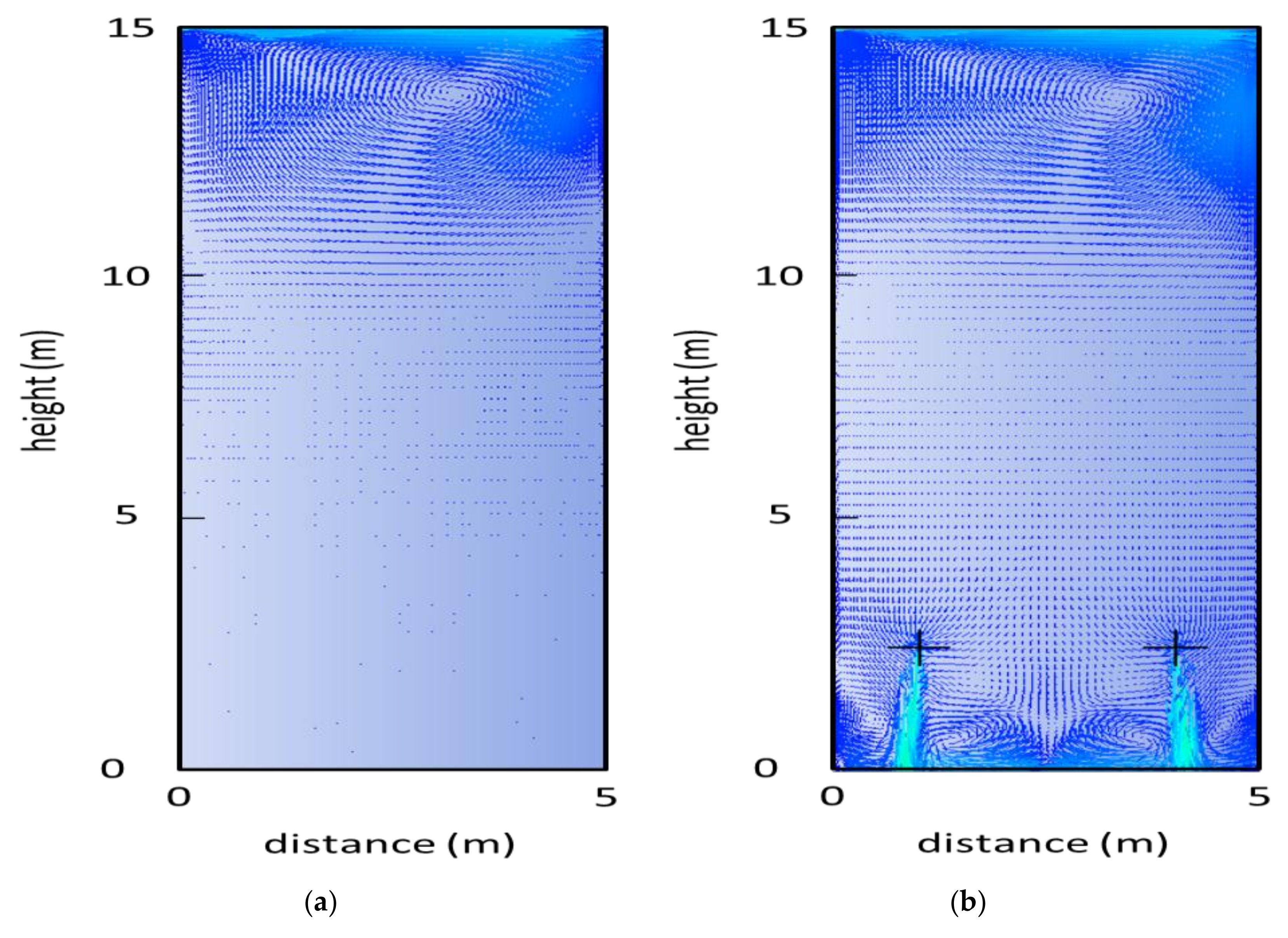
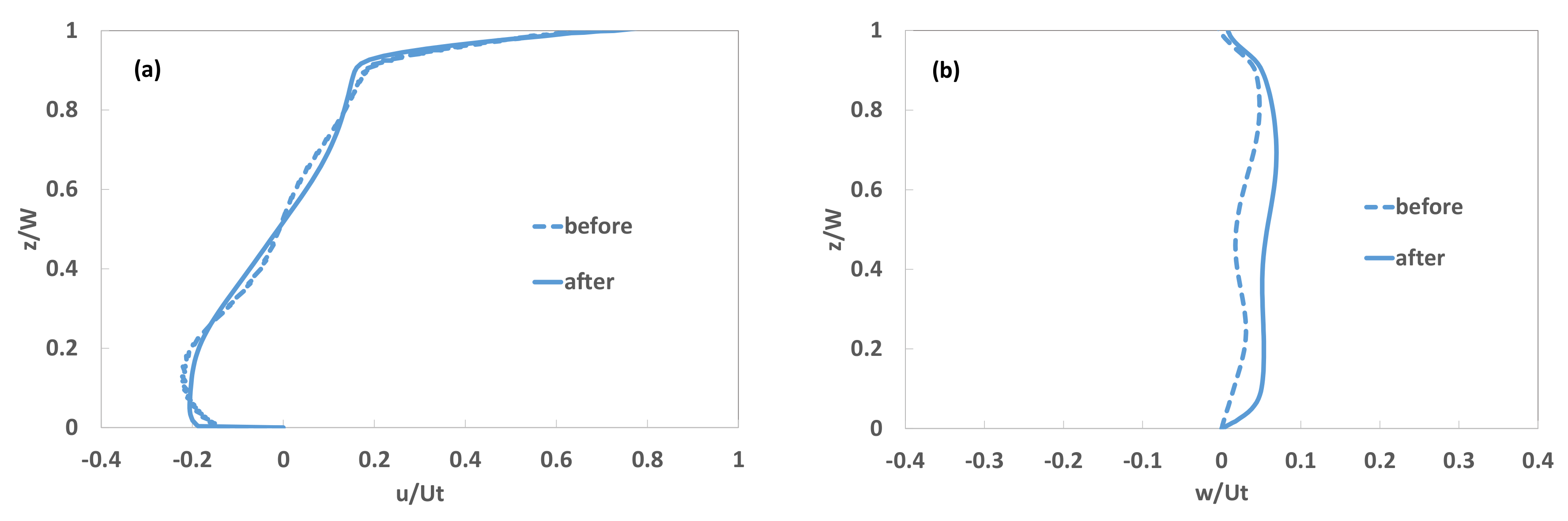
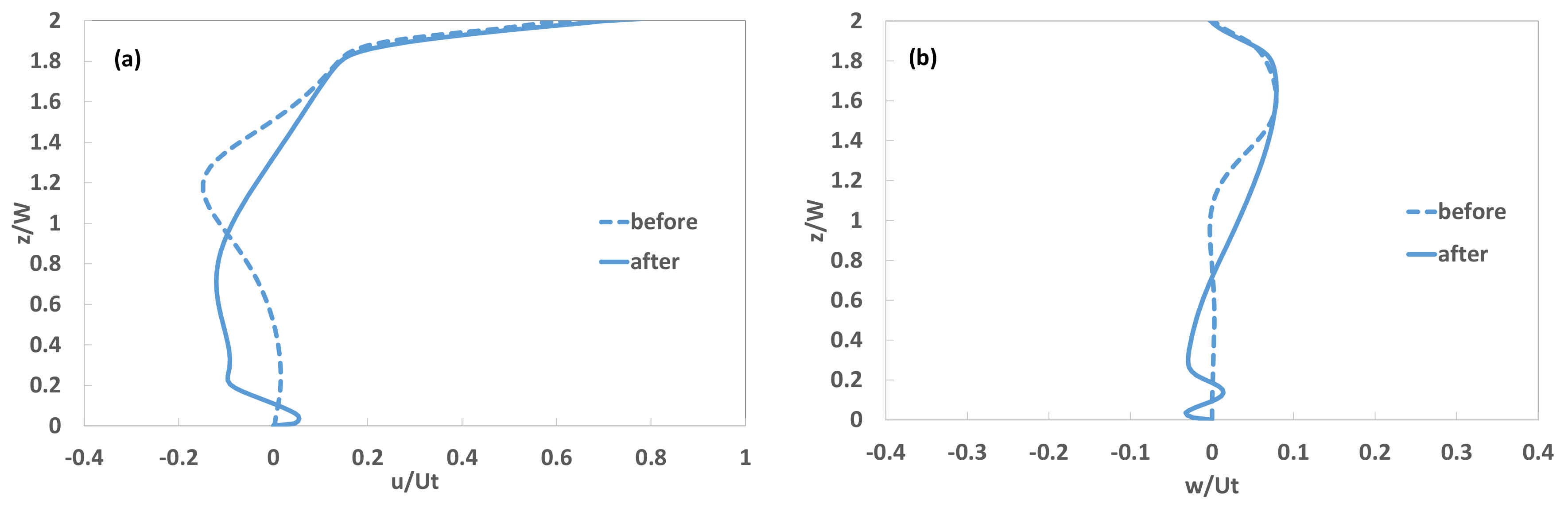
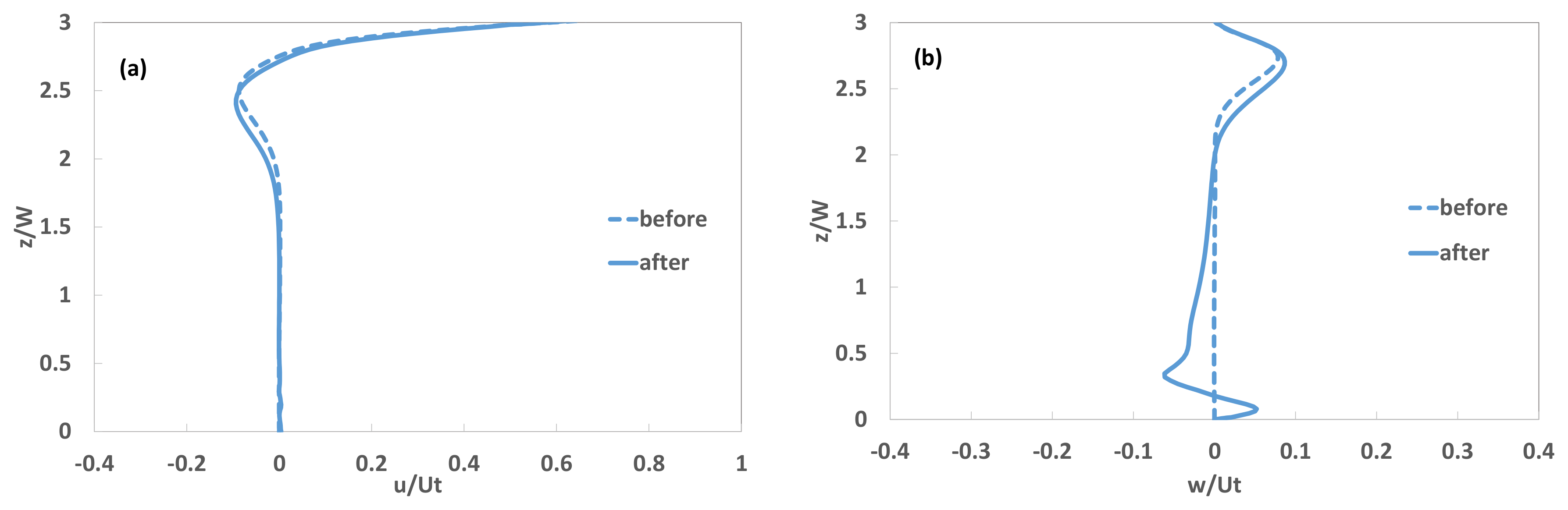
Figure 10 shows the velocity fields in the street canyon before and after the spray nozzles operated for RH = 70% and H/W = 1 (Case 1.1). Figure 11 and Figure 12 are the same as Figure 10 but for H/W = 2 (Case 2.1) and H/W = 3 (Case3.1), respectively. From Figure 10, Figure 11 and Figure 12, we noticed that in the street canyons of H/W = 2 and 3, after the operation of spray systems, the wind velocity fields near the ground were mainly affected by the streams of spray nozzles rather than the wind flowing into the street canyon from outside. Similar results were also observed by Moureh and Yataghene (2016) [19], where the air curtain induced surrounded air flows. This implies that the water spray system (i.e., spray nozzle and water droplet size) would influence the cooling effect in the street canyon as well as the air flow. To further examine the flow field in the street canyon, we plotted the vertical profiles of normalized horizontal velocity (u) and vertical velocity (w) at the middle point (x/W = 0.5, y = 0) before and after spray systems operated for H/W = 1, 2, and 3 in Figure 13, Figure 14 and Figure 15, respectively. These figures showed that, at the middle point of the street canyon, after the operation of spray nozzles, the horizontal and vertical velocities only changed slightly due to the air flow induced by water spray.
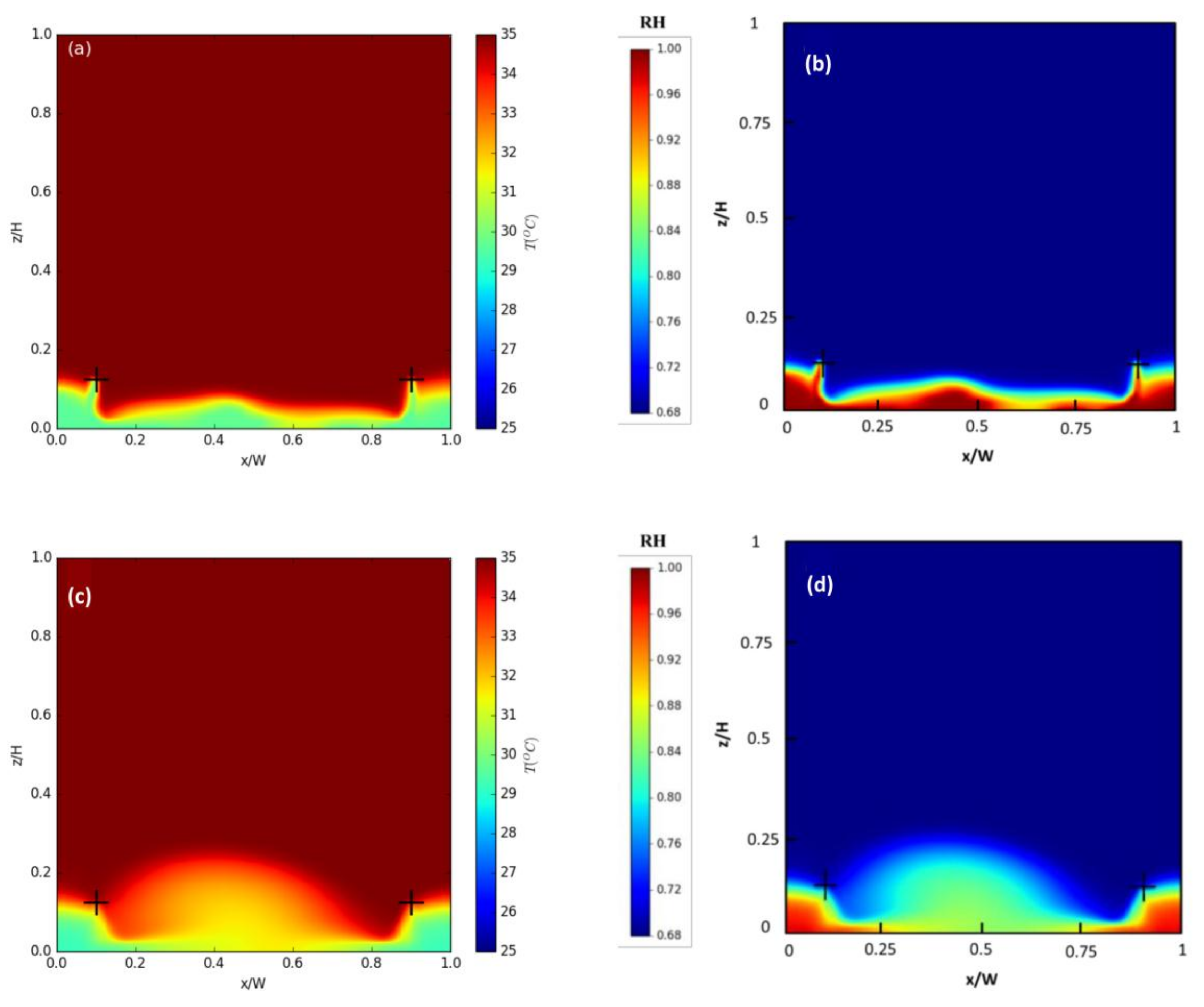
Figure 16 shows the temperature contours on the plane: y = 0 for Case 1.1 (H/W = 1), Case 2.1 (H/W = 2) and Case 3.1 (H/W = 3) at t = 5 s. Figure 17 and Figure 18 also show the temperature contours but at steady state for Cases 1.1, 2.1 and 3.1 (RH = 70%) and Cases 1.2, 2.2 and 3.2 (RH = 80%), respectively. After the spray nozzles started, the water droplets moved to the street canyon bottom due to large (Vw = −15 m/s) negative vertical velocity. Two puffs of colder air cooled by the water droplets merged with each other in the middle of the street canyon. After the two puffs of cooled air merged with each other, the temperature only changed a little and steady state was established.
To check the cooling effect at the average height of a human face (z = 1.5 m, which is also the height of a standard meteorological station), the temperature profiles along the line of y = 0, z = 1.5 in Case 1.1 (H/W = 1, RH = 70%), Case 2.1 (H/W = 2, RH = 70%), Case 3.1 (H/W = 3, RH = 70%), Case 1.2 (H/W = 1, RH = 80%), Case 2.2 (H/W = 2, RH = 80%), and Case 3.2 (H/W = 3, RH = 80%) were plotted in Figure 19. Two distinct regions were noticed in Figure 17, Figure 18, and Figure 19: the region between the nozzle set and the building wall (first region) and the street canyon region between the two nozzle sets (second region). For clarity purposes, the first (I) and second (II) regions were labeled on Figure 18c only. From Figure 19, in region I, just under the nozzles, the air temperature dropped dramatically for all the cases, and reached around the theoretically lowest temperature, which was the wet bulb temperature (discussed later). In region II, regardless of whether there was a condition of RH = 70% or 80%, the cooling effect in cases of H/W = 3 (Case 3.1 and 3.2) were the most efficient (largest temperature drops); cases of H/W = 1 (Case 1.1 and 1.2) were the second; and cases of H/W = 2 (Case 2.1 and 2.2) were the third. The fact that cases of H/W = 1 were better than cases of H/W = 2 was because the air velocity in H/W = 1 was faster. The reason that cases of H/W = 3 had the best cooling performance was due to having the narrowest street canyon.
The average temperatures in regions I and II for Figure 19 are summarized in Table 5. For H/W = 1 and 2, it is clear that the cooling effect is not much (temperature drops between 0.39 to 1.25 °C only) in region II due to a wider street canyon and/or lower air velocity. Figure 19 and Table 5 revealed that the water spray system could only cool the area under the nozzle sets unless the street canyon was narrow.
Also, from Table 5, when the relative humidity changed from 80 to 70%, the average temperature reductions of region II for H/W = 1, 2, and 3 were 0.41, 0.31, and 1.35 °C, respectively. In other words, for region II, when the air is drier, the water spray system could cool the air more only for the cases where the street canyon is narrow. For region I, when the air is drier (RH changed from 80 to 70%), the water spray system could reduce the air temperature more by 1.73, 1.43, and 1.45 °C for H/W = 1, 2, and 3, respectively.
4.2. Effects of Water Droplet Size and Height of Spray Nozzles
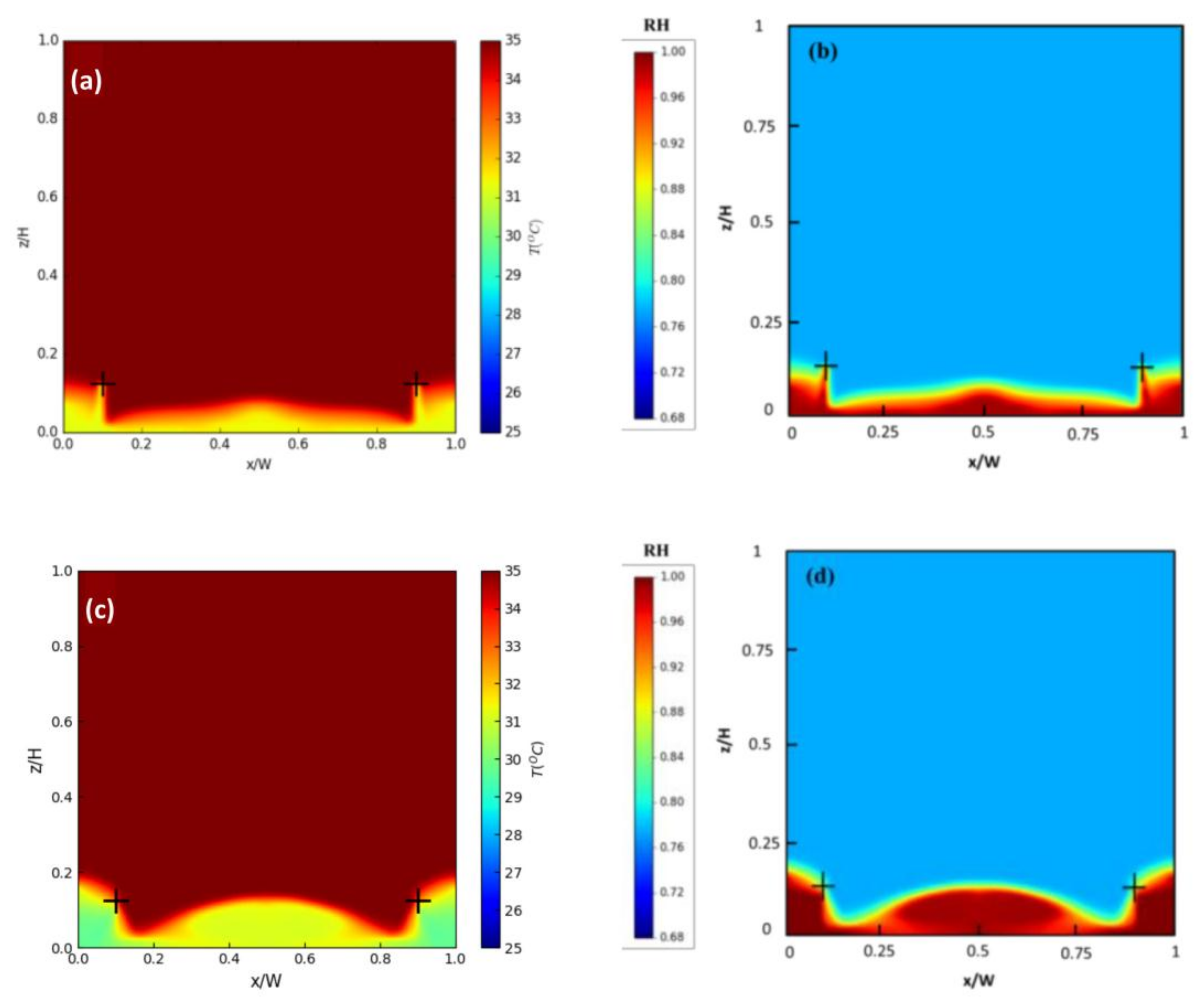
Figure 20 shows the temperature and relative humidity contours on the plane: y = 0 for Case 2.1 (small particle, RH = 70%, = 20 μm, Vw = −15 m/s, = 0.01 kg/s); and Case 2.1a (large particle, RH = 70%, = 369 μm, Vw = −22 m/s, = 0.2 kg/s). Figure 21 is the same as Figure 20 but for Cases 2.2 (small particle, RH = 80%) and 2.2a (large particle, RH = 80%). In Case 2.1, the lowest temperature of the cooled air was about 30 °C, while in Case 2.1a, the lowest temperature was also around 30 °C. However, most of the cooled air in Case 2.1 accumulated at the very bottom of the street canyon. In Case 2.1a, because of the larger velocity of wind caused by the large water droplets from the nozzles, the cooled air in the middle of the street canyon could spread wider (though the cooled air at the very bottom was not saturated by the water droplets). In Figure 21, comparison between Case 2.2 (small particle, RH = 80%) and 2.2a (large particle, RH = 80%) showed similar results as those in Figure 20, but the cooled air in the middle of the street canyon was also saturated by the water droplets in Case 2.2a. This demonstrated that under high humidity conditions (RH ≥ 80%), even large water droplets could saturate the air at the very bottom as the small particles did. The benefit of using large particles was that the cooling area was wider.
Comparison between Figure 20 and Figure 21 suggested that the cooling effect was better when spraying large water droplets into the air than small ones. This was due to the larger velocity and water mass flow rate caused by the large water droplets.
When the air is saturated with water vapor, the air temperature will reach the lowest bound, which is the wet bulb temperature (see Appendix C). Hence, the wet bulb temperature provides an analytical solution of the lowest temperature that the evaporating cooling could reach by spraying water droplets into air. Table 6 lists the wet bulb temperatures solved by Equations (A15) and (A16) under 60, 70, and 80% relative humidity conditions. From Table 6, it is clear that under drier conditions and higher background air temperature, the cooling effect by water spray systems is better.
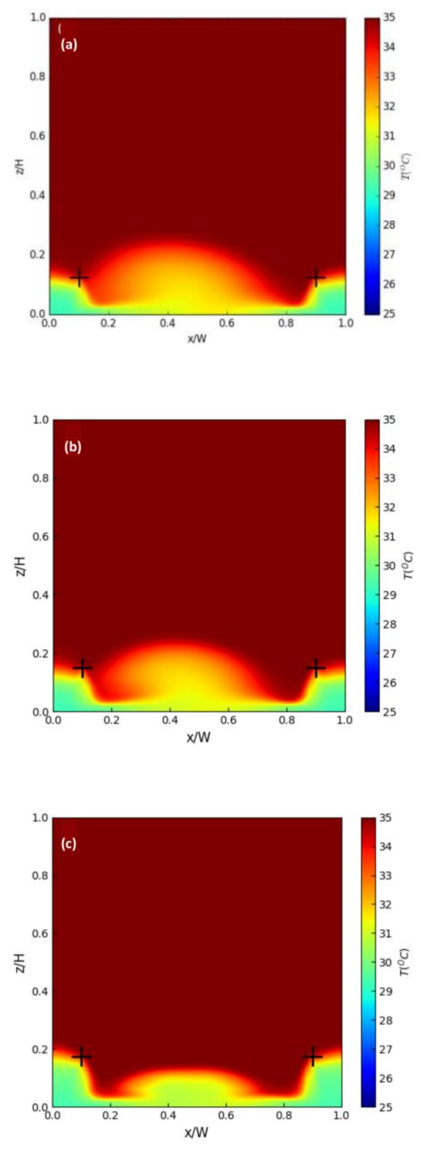
In this study we also investigated the effect of nozzle height on cooling with large water droplets. Figure 22 shows the temperature contours on the plane: y = 0 for Case 2.1a (hs = 2.5 m, = 369 μm), Case 2.1b (hs = 3.0 m, = 369 μm), and 2.1c (hs = 3.5 m, = 369 μm). Comparison in Figure 22 reveals that when the nozzle height was increased (from 2.5 to 3.5 m), the cooling area in the middle of the street canyon was reduced but the reductions in air temperature were about the same. To further examine the cooling effect by increasing the nozzle height, we plotted the horizontal temperature profiles in x-direction at y = 0 and z = 1.5 m for Case 2.1a (hs = 2.5 m), Case 2.1b (hs = 3.0 m), and Case 2.1c (hs = 3.5 m) in Figure 23. For comparison purpose, Case 2.1 (hs = 2.5 m, small water droplets) was also shown in Figure 23. Notice that for all the three large particle cases, the air just under the nozzles at height = 1.5 m all became saturated. However, the temperature differences among these cases at height = 1.5 m were small because the air was almost saturated at this height. This indicated that increasing the nozzle height would not increase the cooling effect at the height of 1.5 m. Figure 23 also demonstrated that using large water droplets has better cooling performance than using the small ones (Case 2.1a vs. Case 2.1).
5. Conclusions
This study simulated the cooling effect of water spray systems in the urban street canyon using the Computational Fluid Dynamics (CFD) method. The 3D unsteady k-ε model coupled with discrete phase model (DPM) provided by ANSYS FLUENT was adopted. The model validation was carried out by flow fields of the urban street canyon measured in water channel experiments [16] and by temperature fields of the wind tunnel experiments [17].
The finding of this study can improve the efficiency of using water spray systems for reducing temperature under different climate conditions and reduce energy demand (including renewable energy) for air conditioning in residential and commercial areas under climate change.
By our simulation results, we conclude the following:
- (1)
- Under region I, the cooling effects were about the same (with a difference of around 1 °C) for different aspect ratios. For region II, H/W = 3 had the best cooling performance, H/W = 1 was the second, and H/W was the third.
- (2)
- Relative humidity has significant influence on the cooling performance. The drier the air, the better the cooling performance of the water spray system is.
- (3)
- The cooling effect was better when spraying large water droplets into the air than small ones. This was due to the larger velocity and water mass flow rate caused by the large water droplets.
- (4)
- Increasing the nozzle height (from 2.5 to 3.5 m) would not increase the cooling effect at the height of 1.5 m.
In summary, if the street width is large (W = 10 or 15 m), the cooled area is just under the spray nozzle. If the street is narrow (W = 5 m), people in the middle of the street also feel the cooling effect.
To extend the application of water spray systems for improving thermal comfort under hot weather (especially in heat waves), future work should focus on how water spray systems would work in wide open areas (e.g., parks, play grounds, outdoor food courts). Understanding the cooling effect of water spray systems with manipulation of other controlling variables, like nozzle spray angle, ambient wind velocity, and incoming radiation, is also needed.
Acknowledgments
This work was supported by the Ministry of Science and Technology, Taiwan [grant number: 99-2111-M-002-004-MY3].
Author Contributions
Y.-C. L. and C.-I H. conceived the research design; Y.-C. L. performed the model simulations; Y.-C. L., T.-J. C. and C.-I H. analyzed and interpreted the data; Y.-C. L. and C.-I H. wrote the paper.
Conflicts of Interest
The authors declare no conflict of interest.
Appendix A. Governing Equations of the Continuous Phase
The continuous phase model is solved based on the mass, momentum, and energy conservation principles. Reynolds averaging—which considers the transport of mean velocity (Ui), turbulence kinetic energy (k), and kinetic energy dissipation rate (ε)—is used to solve the turbulence flow. In this study, the Re-Normalized Group (RNG) k-ε is used. The governing equations are:
The mass conservation equation (for incompressible flow):
where Sm is the source term of mass that is added to continuous phase because of the evaporation of water (kg/m3 s).
The momentum conservation equation:
where is the velocity fluctuation in the i direction (m/s), ν is molecular kinematic viscosity (m2/s), g is gravity acceleration (m/s2), νt is turbulent kinematic viscocity (m2/s), Cμ is a constant which is 0.0845 in RNG k-ε model, Fi is the source term of force in the i direction exerted on continuous phase by discrete phase (water droplets) and is described by Equation (A9).
The conservation of turbulence kinetic energy (k) and kinetic energy dissipation rate (ε):
where and αϵ are the inverse effective Prantl numbers and are both around 1.393, is effective turbulent kinematic viscocity (), and
β is the thermal expansion coefficient in the form: 1/ρ (∂ρ/∂T). , Sk is the scalar measure of the deformation tensor, and a are 4.38 and 0.012, respectively, and .
Water vapor mass conservation:
where Dm is molecular diffusivity (m2/s), Dt is turbulent diffusivity (m2/s), which can be obtained by where Sct (=0.7) is the turbulent Schmidt number. Sv is the source term due to the evaporation of the droplet in discrete particle model.
Energy conservation equation:
where Prt (turbulent Prandtl number) is 0.85, Sh is source term which is contributed by latent heat absorbed during the evaporation of droplets. E is total energy of the fluid (J/kg/m3) defined as:
Appendix B. Governing Equations of the Discrete Phase (Water Droplets)
(1) Particle force balance:
where is the particle velocity (m/s), is the air velocity (m/s), is the molecular viscosity of the air (kg/m/s), is the density of particle (kg/m3), is the diameter of particle (m), is the drag coefficient, is the density of air (kg/m3), is gravity acceleration (m/s2), Re is the droplet Reynolds number, which is defined by .
Here, the water droplets are assumed to be spherical particles, and the drag coefficient of spherical particles is:
where , , and are constants given with different ranges of Re [20].
(2) Particle mass transfer:
The water droplets evaporate and transfer the mass into the air. The water droplets are modeled as particles surrounded by saturated air-vapor films; when the concentration of water vapor in the films is larger than that in the air, the gradient causes the water vapor to diffuse from the film to the air.
The mass transfer rate is as below:
where is the mass of the particle (kg), is the molecular weight of the particle (kg/mol), is the surface area of the particle (m2), is the mass transfer coefficient (m/s), is the vapor concentration at the surface (saturated air-vapor film) (mol/m3), and is calculated by: , where is the saturated vapor pressure at the particle temperature (Tp), R is the universal gas constant, is the vapor concentration in the air (mol/m3). Kc is calculated from the empirical correlation of Sherwood number [21]:
where Sh is the Sherwood number; D is the diffusion coefficient of vapor (m2/s); Sc is the Schmidt number, which is given as: .
(3) Particle heat transfer:
where is the specific heat of water droplet (J/kg), is the latent heat of water (kJ/mol), is the convection heat transfer coefficient, which was calculated from the empirical correlation of Nu number when vapor mass fraction << 1 [22]:
where is the thermal conductivity of the continuous phase, Pr is the Prandtl number of the continuous phase, which is given as: .
Appendix C. Wet Bulb Temperature
The wet bulb temperature is the temperature that an air parcel would reach when it was cooled and saturated by the evaporation of water. Hence, the wet bulb temperature is the lowest temperature that the air can reach when cooled by evaporative cooling. By energy conservation, the wet bulb temperature can be determined with [23]:
where Ta is the air temperature, Tw is wet bulb temperature, Cp is the specific heat of air (29.3 J/mol/K), es (Tw) is the saturate vapor pressure (kPa) at Tw, ea is the initial vapor pressure at Ta, Pa is air pressure (kPa), λ is the latent heat of water (J/mol). es(Tw) can be calculated by:
(Ta − Tw)Cp = [(es(Tw) − ea)/Pa] λ
The wet bulb temperature can be found by solving (A15) and (A16) together.
References
- Sarrat, C.; Lemonsu, A.; Masson, V.; Guedalia, D. Impact of urban heat island on regional atmospheric pollution. Atmos. Environ. 2006, 40, 1743–1758. [Google Scholar] [CrossRef]
- Kovats, R.S.; Hajat, S. Heat stress and public health: A critical review. Ann. Rev. Public Health 2008, 29, 41–55. [Google Scholar] [CrossRef] [PubMed]
- Isaac, M.; Van Vuuren, D.P. Modeling global residential sector energy demand for heating and air conditioning in the context of climate change. Energy Policy 2009, 37, 507–521. [Google Scholar] [CrossRef]
- Alexandri, E.; Jones, P. Temperature decreases in an urban canyon due to green walls and green roofs in diverse climates. Build. Environ. 2008, 43, 480–493. [Google Scholar] [CrossRef]
- Runsheng, T.; Etzion, Y.; Erell, E. Experimental studies on a novel roof pond configuration for the cooling of buildings. Renew. Energy 2003, 28, 1513–1522. [Google Scholar] [CrossRef]
- Montazeri, H.; Blocken, B.; Hensen, J.L.M. Evaporative cooling by water spray systems: CFD simulation, experimental validation and sensitivity analysis. Build. Environ. 2015, 83, 129–141. [Google Scholar] [CrossRef]
- Montazeri, H.; Toparlar, Y.; Blocken, B.; Hensen, J.L.M. Simulating the cooling effects of water spray systems in urban landscapes: A computational fluid dynamics study in Rotterdam, The Netherlands. Landsc. Urban Plan. 2017, 159, 85–100. [Google Scholar] [CrossRef]
- Jain, S.P.; Rao, K.R. Experimental study on the effect of roof spray cooling on unconditioned and conditioned buildings. Build. Sci. 1974, 9, 9–16. [Google Scholar] [CrossRef]
- Huang, C.; Ye, D.; Zhao, H.; Liang, T.; Lin, Z.; Yin, H.; Yang, Y. The research and application of spray cooling technology in Shanghai Expo. Appl. Therm. Eng. 2011, 31, 3726–3735. [Google Scholar] [CrossRef]
- Kang, D.; Strand, R.K. Modeling of simultaneous heat and mass transfer within passive down-draft evaporative cooling (PDEC) towers with spray in FLUENT. Energy Build. 2013, 62, 196–209. [Google Scholar] [CrossRef]
- Baik, J.J.; Kim, J.J. A numerical study of flow and pollutant dispersion characteristics in urban street canyons. J. Appl. Meteorol. 1999, 38, 1576–1589. [Google Scholar] [CrossRef]
- Chan, T.L.; Dong, G.; Leung, C.W.; Cheung, C.S.; Hung, W.T. Validation of a two-dimensional pollutant dispersion model in an isolated street canyon. Atmos. Environ. 2002, 36, 861–872. [Google Scholar] [CrossRef]
- ANSYS Inc. ANSYS Fluent 15.0 Theory Guide; ANSYS Inc.: Canonsburg, PA, USA, 2013. [Google Scholar]
- Launder, B.E.; Spalding, D.B. The numerical computation of turbulent flows. Comput. Methods Appl. Mech. Eng. 1974, 3, 269–289. [Google Scholar] [CrossRef]
- Rosin, P.; Rammler, E. The laws governing the fineness of powdered coal. J. Inst. of Fuel 1933, 31, 29–36. [Google Scholar]
- Baik, J.J.; Park, R.S.; Chun, H.Y.; Kim, J.J. A laboratory model of urban street-canyon flows. J. Appl. Meteorol. 2000, 39, 1592–1600. [Google Scholar] [CrossRef]
- Sureshkumar, R.; Kale, S.R.; Dhar, P.L. Heat and mass transfer processes between a water spray and ambient air—I. Experimental data. Appl. Therm. Eng. 2008, 28, 349–360. [Google Scholar] [CrossRef]
- Sureshkumar, R.; Kale, S.R.; Dhar, P.L. Heat and mass transfer processes between a water spray and ambient air—II Simulations. Appl. Therm. Eng. 2008, 28, 361–371. [Google Scholar] [CrossRef]
- Moureh, J.; Yataghene, M. Numerical and experimental study of airflow patterns and global exchanges through an air curtain subjected to external lateral flow. Exp. Therm. Fluid Sci. 2016, 74, 308–323. [Google Scholar] [CrossRef]
- Morsi, S.; Alexander, A.J. An investigation of particle trajectories in two-phase flow systems. J. Fluid Mech. 1972, 55, 193–208. [Google Scholar] [CrossRef]
- Ranz, W.E.; Marshall, W.R. Evaporation from drops. Chem. Eng. Prog 1952, 48, 141–146. [Google Scholar]
- Sazhin, S.S. Advanced models of fuel droplet heating and evaporation. Prog. Energy Combust. Sci. 2006, 32, 162–214. [Google Scholar] [CrossRef]
- Campbell, G.S.; Norman, J.M. An introduction to Environmental Biophysics; Springer Science & Business Media: New York, NY, USA, 1998; p. 44. [Google Scholar]
Figure 1.
Computational geometry for the street canyon (a) H/W = 1 (b) H/W = 2 (c) H/W = 3.
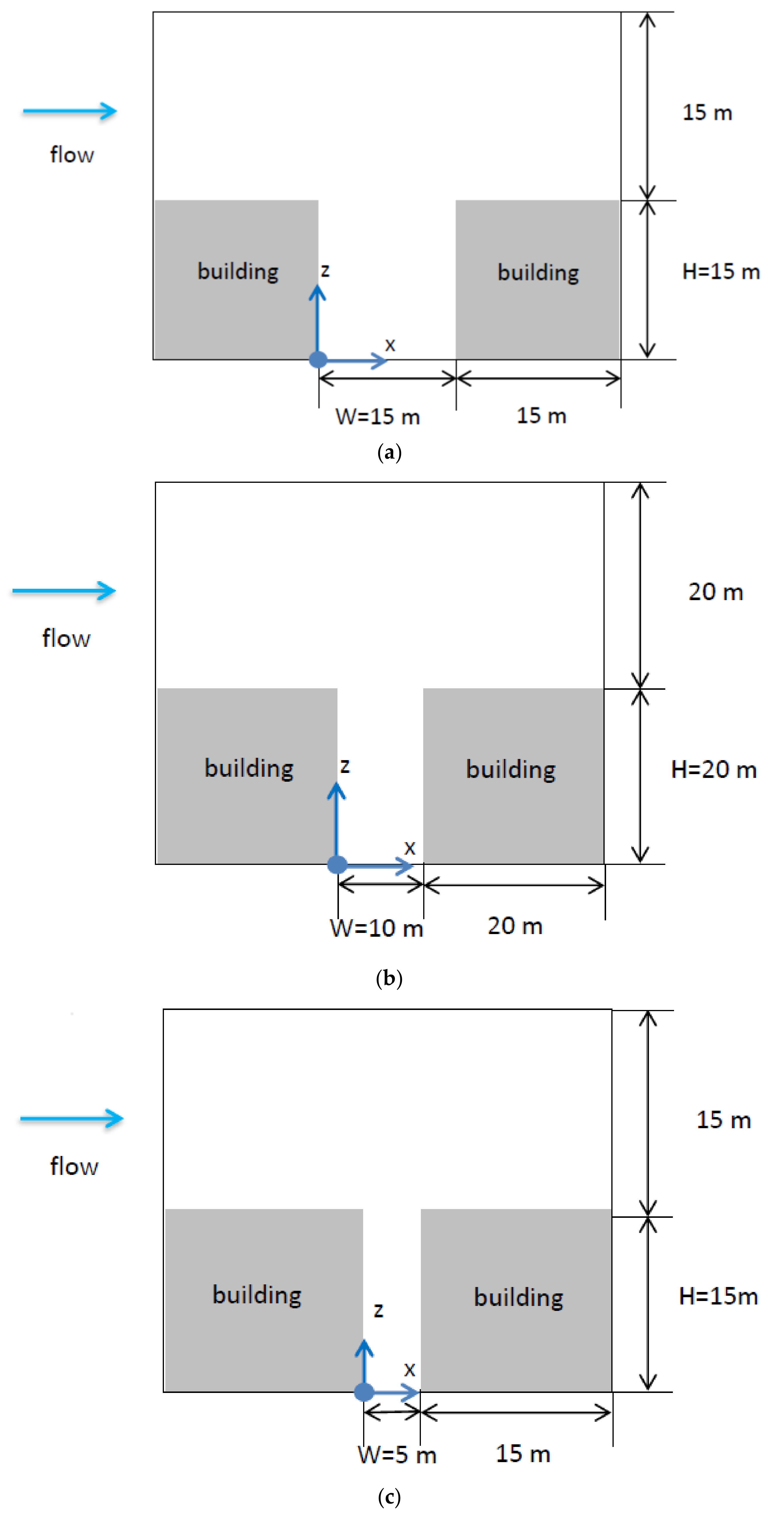
Figure 2.
Computational meshes for the street canyon (a) H/W = 1 (b) H/W = 2 (c) H/W = 3.
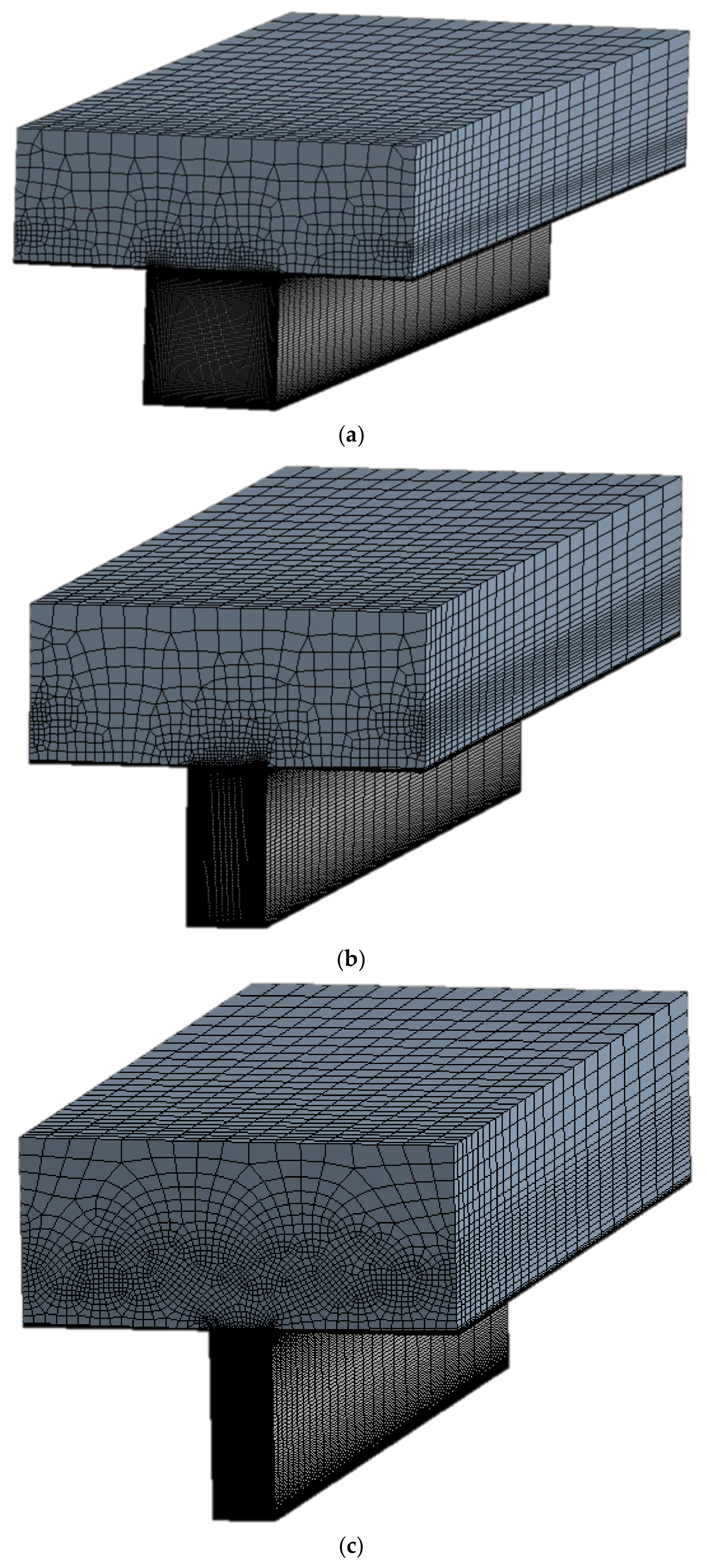
Figure 3.
(a) Layout of a set of spray nozzles; (b) Positions of the two nozzle sets in the street canyon. The two nozzle sets were located at 2.5 m height and 1 m away from each building wall. The y positions of the 7 nozzles were ±1.5, ±1, ±0.5, and 0, respectively.
Figure 3.
(a) Layout of a set of spray nozzles; (b) Positions of the two nozzle sets in the street canyon. The two nozzle sets were located at 2.5 m height and 1 m away from each building wall. The y positions of the 7 nozzles were ±1.5, ±1, ±0.5, and 0, respectively.

Figure 4.
(a) Mass distribution and (b) Number distribution of water droplets as a function of droplet diameter with the mean diameter μm
Figure 4.
(a) Mass distribution and (b) Number distribution of water droplets as a function of droplet diameter with the mean diameter μm


Figure 5.
(a) Mass distribution and (b) Number distribution of water droplets as a function of droplet diameter with the mean diameter μm
Figure 5.
(a) Mass distribution and (b) Number distribution of water droplets as a function of droplet diameter with the mean diameter μm
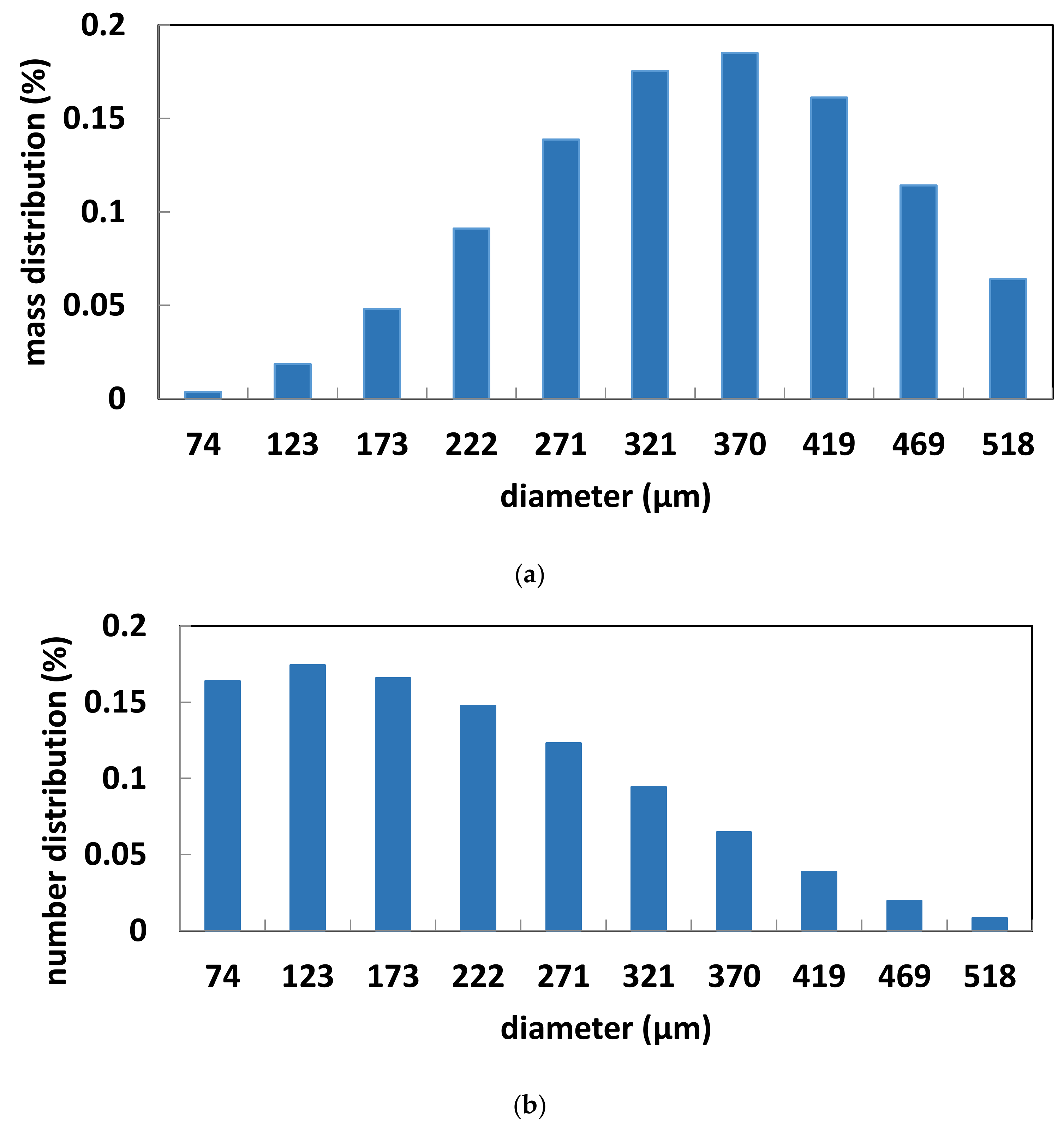
Figure 6.
Normalized vertical velocity as a function of normalized height at upstream (x/W = 0.125), middle (x/W = 0.5), and downstream positions (x/W = 0.875). w is the vertical velocity and Ut is the x direction velocity just above the top of the building. (a) H/W = 1; (b) H/W = 2. Open circle denotes the measurement by Baik et al., (2000) [16]; dash line denotes the prediction by Baik and Kim (1999) [11]; solid line denotes the prediction by this study.
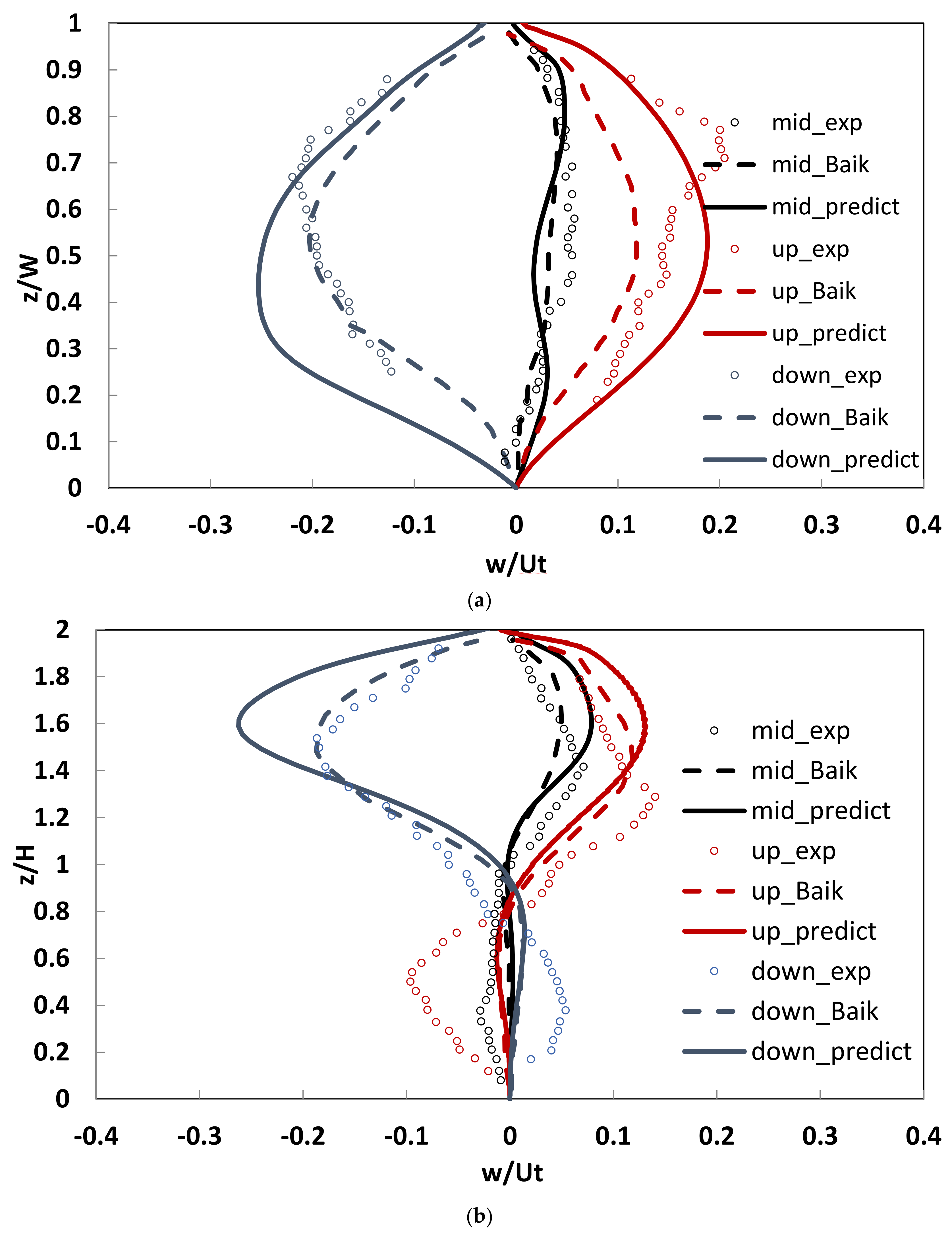
Figure 7.
Normalized horizontal velocity as a function of normalized height at upstream (x/W = 0.125), middle (x/W = 0.5), and downstream positions (x/W = 0.875). u is the horizontal velocity and Ut is the x direction velocity just above the top of the building. (a) H/W = 1; (b) H/W = 2. Open circle denotes the measurement by Baik et al., (2000) [16]; dash line denotes the prediction by Baik and Kim (1999) [11]; solid line denotes the prediction by this study. Measurements of horizontal velocity were derived from Figure 3a, Figure 4, Figure 6a and Figure 7 of Baik et al., (2000) [16] by the authors.

Figure 8.
The relative positions of temperature measurement and the spray nozzle in the wind tunnel experiment by Sureshkumar et al., (2008) [17]. The dimension of the test section is 1.9 m × 0.585 m × 0.585 m.
Figure 8.
The relative positions of temperature measurement and the spray nozzle in the wind tunnel experiment by Sureshkumar et al., (2008) [17]. The dimension of the test section is 1.9 m × 0.585 m × 0.585 m.

Figure 9.
Comparison of model predictions and measurements. (a) Dry bulb temperature (DBT, °C) (b) Specific humidity (g/g).
Figure 9.
Comparison of model predictions and measurements. (a) Dry bulb temperature (DBT, °C) (b) Specific humidity (g/g).

Figure 10.
Velocity field in the street canyon before spray systems operated (a) and after spray systems operated (b) for H/W = 1. The black cross indicates the position of water spray system. The maximum velocity vector length corresponds to 0.98 m/s in Figure 10a, and 1.36 m/s in Figure 10b.
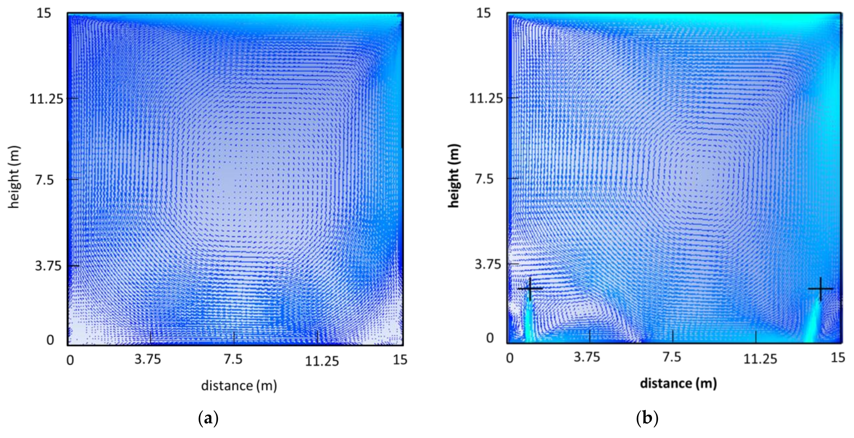
Figure 11.
Velocity field in the street canyon before spray systems operated (a) and after spray systems operated (b) for H/W = 2. The black cross indicates the position of the water spray system. The maximum velocity vector length corresponds to 0.94 m/s in Figure 11a, and 1.31 m/s in Figure 11b.
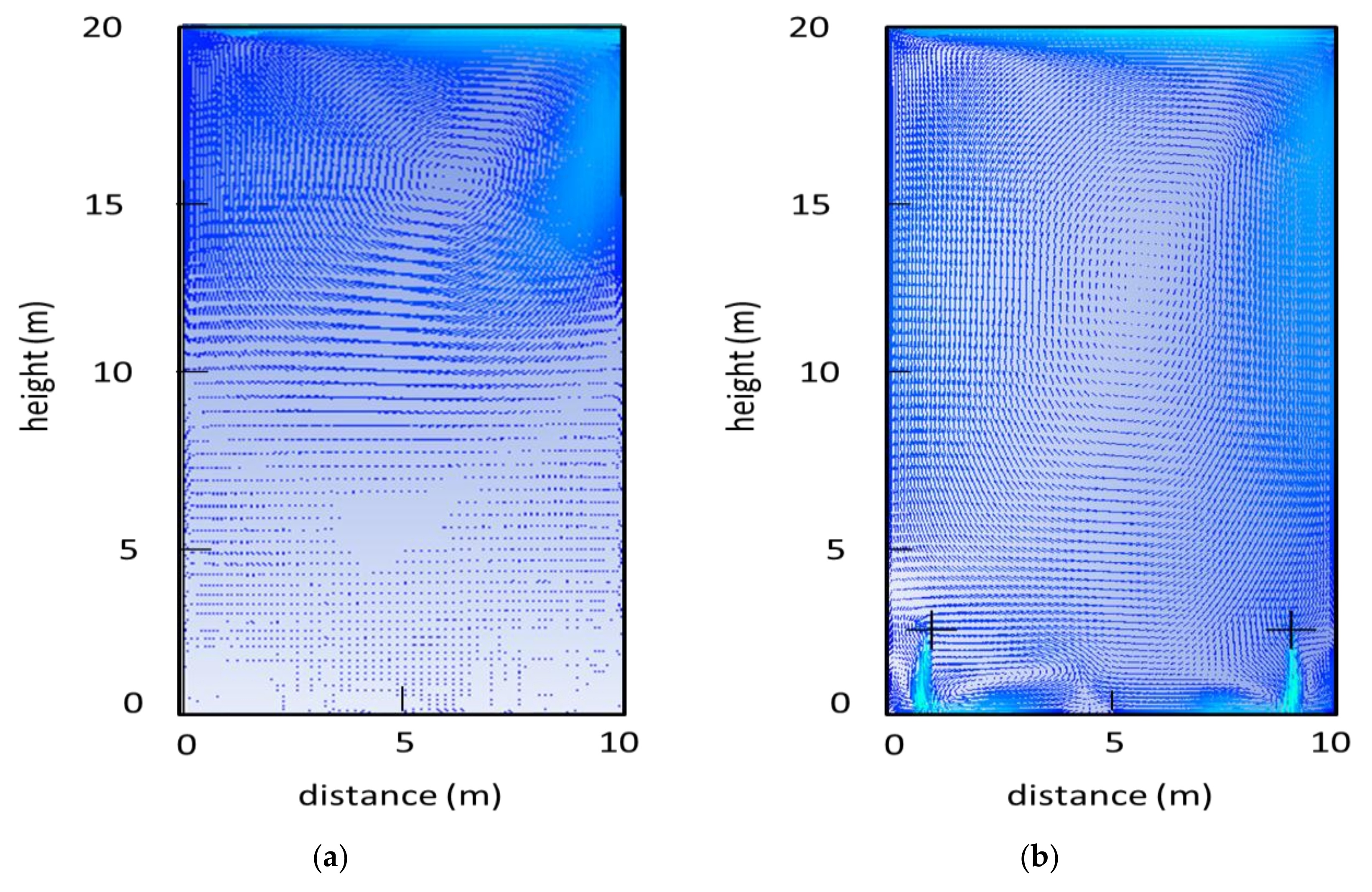
Figure 12.
Velocity field in the street canyon before spray systems operated (a) and after spray systems operated (b) for H/W = 3. The black cross indicates the position of water spray system. The maximum velocity vector length corresponds to 0.84 m/s in Figure 12a, and 1.36 m/s in Figure 12b.

Figure 13.
Vertical profile of normalized horizontal velocity (a) and vertical velocity (b) at x/W = 0.5 and y = 0 before and after spray systems operated for H/W = 1. Ut is the x direction velocity just above the top of the building.
Figure 13.
Vertical profile of normalized horizontal velocity (a) and vertical velocity (b) at x/W = 0.5 and y = 0 before and after spray systems operated for H/W = 1. Ut is the x direction velocity just above the top of the building.

Figure 14.
Vertical profile of normalized horizontal velocity (a) and vertical velocity (b) at x/W = 0.5 and y = 0 before and after spray systems operated for H/W = 2. Ut is the x direction velocity just above the top of the building.
Figure 14.
Vertical profile of normalized horizontal velocity (a) and vertical velocity (b) at x/W = 0.5 and y = 0 before and after spray systems operated for H/W = 2. Ut is the x direction velocity just above the top of the building.

Figure 15.
Vertical profile of normalized horizontal velocity (a) and vertical velocity (b) at x/W = 0.5 and y = 0 before and after spray systems operated for H/W = 3. Ut is the x direction velocity just above the top of the building.
Figure 15.
Vertical profile of normalized horizontal velocity (a) and vertical velocity (b) at x/W = 0.5 and y = 0 before and after spray systems operated for H/W = 3. Ut is the x direction velocity just above the top of the building.

Figure 16.
Temperature contour in the street canyon on the plane: y = 0 and t = 5 s. The black cross indicates the position of water spray system. (a) Case 1.1 (H/W = 1); (b) Case 2.1 (H/W = 2); (c) Case 3.1 (H/W = 3).
Figure 16.
Temperature contour in the street canyon on the plane: y = 0 and t = 5 s. The black cross indicates the position of water spray system. (a) Case 1.1 (H/W = 1); (b) Case 2.1 (H/W = 2); (c) Case 3.1 (H/W = 3).
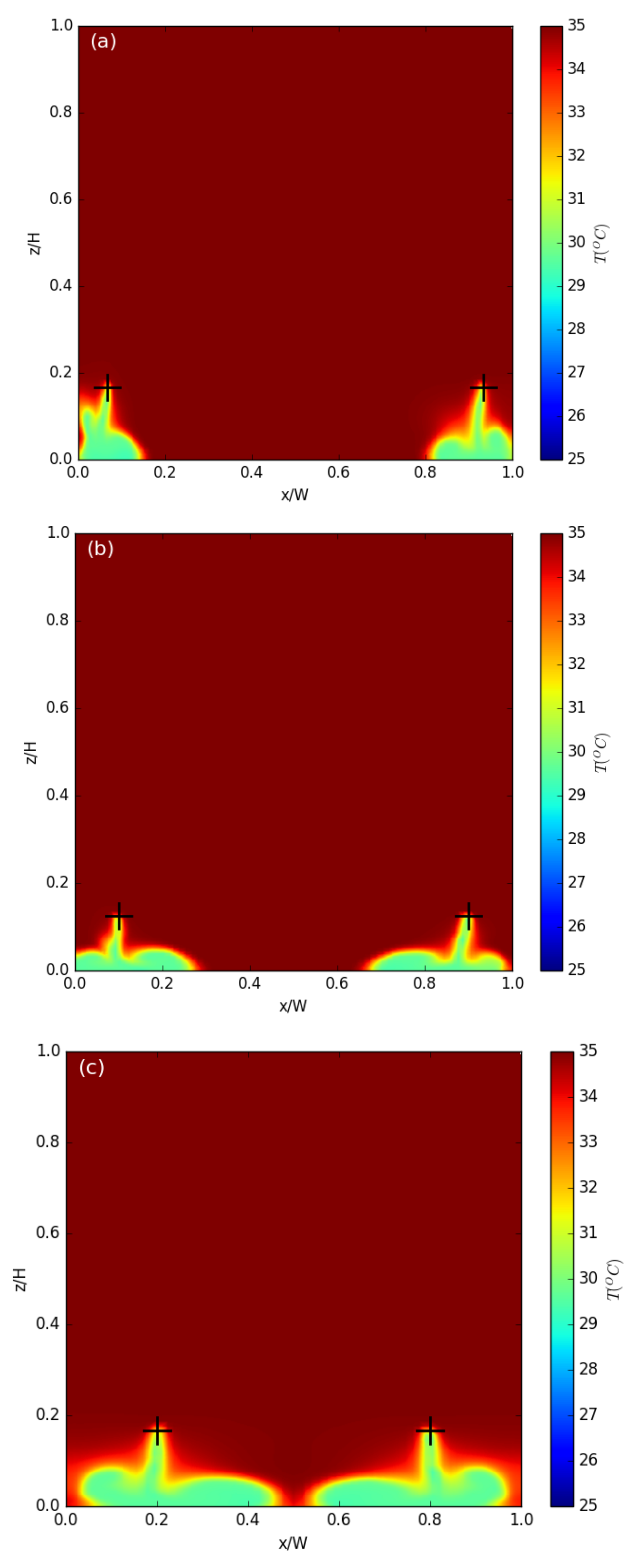
Figure 17.
Temperature contour in the street canyon on the plane: y = 0 when steady state was reached. The black cross indicates the position of water spray system. (a) Case 1.1 (H/W = 1, RH = 70%); (b) Case 2.1 (H/W = 2, RH = 70%); (c) Case 3.1 (H/W = 3, RH = 70%).
Figure 17.
Temperature contour in the street canyon on the plane: y = 0 when steady state was reached. The black cross indicates the position of water spray system. (a) Case 1.1 (H/W = 1, RH = 70%); (b) Case 2.1 (H/W = 2, RH = 70%); (c) Case 3.1 (H/W = 3, RH = 70%).
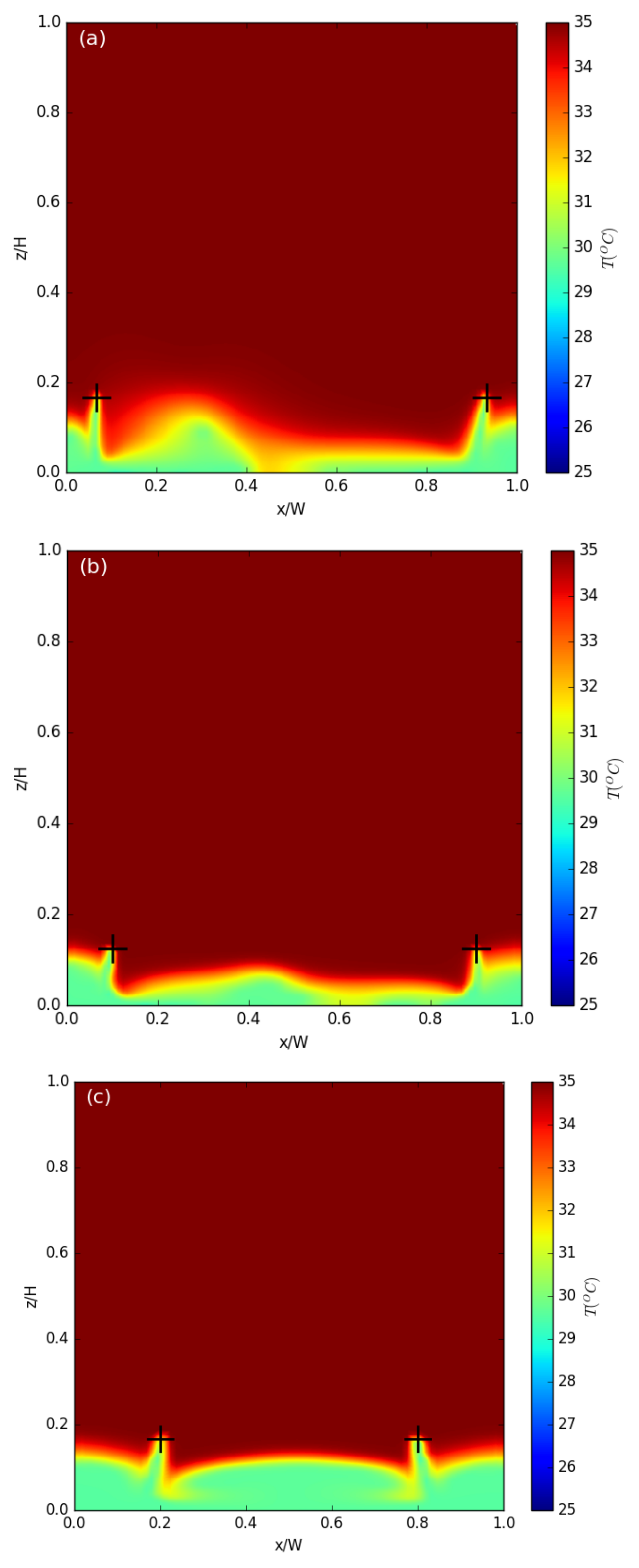
Figure 18.
Temperature contour in the street canyon on the plane: y = 0 when steady state was reached. The black cross indicates the position of water spray system. (a) Case 1.2 (H/W = 1, RH = 80%); (b) Case 2.2 (H/W = 2, RH = 80%); (c) Case 3.2 (H/W = 3, RH = 80%).
Figure 18.
Temperature contour in the street canyon on the plane: y = 0 when steady state was reached. The black cross indicates the position of water spray system. (a) Case 1.2 (H/W = 1, RH = 80%); (b) Case 2.2 (H/W = 2, RH = 80%); (c) Case 3.2 (H/W = 3, RH = 80%).
Figure 19.
Temperature profile on the line: y = 0, z = 1.5 m under different aspect ratios and Relative humidity: Case 1.1 (H/W = 1, RH = 70%), Case 2.1 (H/W = 2, RH = 70%), Case 3.1 (H/W = 3, RH = 70%), Case 1.2 (H/W = 1, RH = 80%), Case 2.2 (H/W = 2, RH = 80%), Case 3.2 (H/W = 3, RH = 80%). The background temperature was 35 °C
Figure 20.
(a) Temperature and (b) relative humidity contour on the plane: y = 0 for Case 2.1 (small particle, = 20 μm, RH = 70%); (c) Temperature and (d) relative humidity contour on the plane: y = 0 for Case 2.1a (large particle, = 369 μm, RH = 70%).
Figure 20.
(a) Temperature and (b) relative humidity contour on the plane: y = 0 for Case 2.1 (small particle, = 20 μm, RH = 70%); (c) Temperature and (d) relative humidity contour on the plane: y = 0 for Case 2.1a (large particle, = 369 μm, RH = 70%).

Figure 21.
(a) Temperature and (b) relative humidity contour on the plane: y = 0 for Case 2.2 (small particle, = 20 μm, RH = 80%); (c) Temperature and (d) relative humidity contour on the plane: y = 0 for Case 2.2a (large particle, = 369 μm, RH = 80%).
Figure 21.
(a) Temperature and (b) relative humidity contour on the plane: y = 0 for Case 2.2 (small particle, = 20 μm, RH = 80%); (c) Temperature and (d) relative humidity contour on the plane: y = 0 for Case 2.2a (large particle, = 369 μm, RH = 80%).

Figure 22.
Temperature contour on the plane: y = 0 (a) Case 2.1a (hs = 2.5 m, large particle, = 369 μm, RH = 70%); (b) Case 2.1b (hs = 3.0 m, large particle, = 369 μm, RH = 70%); (c) for Case 2.1c (hs = 3.5 m, large particle, = 369 μm, RH = 70%).
Figure 22.
Temperature contour on the plane: y = 0 (a) Case 2.1a (hs = 2.5 m, large particle, = 369 μm, RH = 70%); (b) Case 2.1b (hs = 3.0 m, large particle, = 369 μm, RH = 70%); (c) for Case 2.1c (hs = 3.5 m, large particle, = 369 μm, RH = 70%).

Figure 23.
Temperature profile on the line: y = 0, z = 1.5 m under different height of spray nozzles (large particle, hs = 2.5, 3.0, 3.5 m). The background temperature was 35 °C. For comparison purposes, Case 2.1 (small particle, hs = 2.5 m) was also shown.
Figure 23.
Temperature profile on the line: y = 0, z = 1.5 m under different height of spray nozzles (large particle, hs = 2.5, 3.0, 3.5 m). The background temperature was 35 °C. For comparison purposes, Case 2.1 (small particle, hs = 2.5 m) was also shown.

Table 1.
Summary of the CFD model parameters and nozzle characteristics.
| Roughness of No-Slip Boundary | Time Step Size (sec) | Characteristics of the Spray Nozzle | |||||
|---|---|---|---|---|---|---|---|
| ks | Cs | Continuous Phase | Particle Phase | α/2 | Points of Injection | Radius | Tw |
| 1.5 | 0.5 | 0.05 | 0.001 | 20° | 15 | 2 mm | 25 °C |
ks is the roughness height of the buildings and street; Cs is the roughness constant of the buildings and street; α/2 is the half cone angle of the nozzle; Tw is water temperature.
Table 2.
List of the parameters of the study cases.
| Group | Case | H/W | RH (%) | hs (m) | Vw (m/s) | (kg/s) | (μm) | Dmin (μm) | Dmax (μm) |
|---|---|---|---|---|---|---|---|---|---|
| # 1 (different H/W and RH) | 1.1 | 1 | 70 | 2.5 | −15 | 0.01 | 20 | 10 | 60 |
| 2.1 | 2 | 70 | 2.5 | −15 | 0.01 | 20 | 10 | 60 | |
| 3.1 | 3 | 70 | 2.5 | −15 | 0.01 | 20 | 10 | 60 | |
| 1.2 | 1 | 80 | 2.5 | −15 | 0.01 | 20 | 10 | 60 | |
| 2.2 | 2 | 80 | 2.5 | −15 | 0.01 | 20 | 10 | 60 | |
| 3.2 | 3 | 80 | 2.5 | −15 | 0.01 | 20 | 10 | 60 | |
| # 2 (different RH and ) | 2.1 | 2 | 70 | 2.5 | −15 | 0.01 | 20 | 10 | 60 |
| 2.1a | 2 | 70 | 2.5 | −22 | 0.2 | 369 | 74 | 518 | |
| 2.2 | 2 | 80 | 2.5 | −15 | 0.01 | 20 | 10 | 60 | |
| 2.2a | 2 | 80 | 2.5 | −22 | 0.2 | 369 | 74 | 518 | |
| # 3 (different hs) | 2.1a | 2 | 70 | 2.5 | −22 | 0.2 | 369 | 74 | 518 |
| 2.1b | 2 | 70 | 3 | −22 | 0.2 | 369 | 74 | 518 | |
| 2.1c | 2 | 70 | 3.5 | −22 | 0.2 | 369 | 74 | 518 |
Group #1: to analyze the effects of the street canyon aspect ratio (H/W) and relative humidity (RH), we consider H/W = 1, 2 and 3, and RH = 70 and 80% with small water droplets (mean water droplet diameter = 20 μm) and the nozzle height set at 2.5 m above the ground. These cases were Case 1.1, 2.1, 3.1, and 1.2, 2.2, 3.2, respectively; Group #2: to explore the effects of the water droplet size under different levels of relative humidity, we consider small and larger water droplets ( = 20 and 369 μm, respectively) under RH = 70 and 80% with H/W = 2 and hs = 2.5 m above the ground. These cases were Case 2.1, 2.1a and 2.2, 2.2a, respectively; Group #3: for studying the effect of the spray nozzle height (hs), we considered hs = 2.5, 3.0, and 3.5 m above the ground, under H/W = 2, RH = 70% and = 369 μm. These cases were Case 2.1a, 2,1b and 2.1c, respectively.
Table 3.
The linear regression and root mean square error (RMSE) of vertical velocity between the experimental data and model predictions by Baik and Kim (1999) [11] and present study.
Table 3.
The linear regression and root mean square error (RMSE) of vertical velocity between the experimental data and model predictions by Baik and Kim (1999) [11] and present study.
| H/W = 1 | Linear Regression | R2 | RMSE |
| Baik and Kim (1999) | y = 0.794 x − 0.0153 | 0.9645 | 1.06 |
| This study | y = 1.126 x − 0.0068 | 0.9524 | 1.51 |
| H/W = 2 | Linear Regression | R2 | RMSE |
| Baik and Kim (1999) | y = 0.765 x − 0.0024 | 0.7678 | 0.55 |
| This study | y = 0.860 x + 0.0023 | 0.6699 | 0.66 |
‘x’ in the linear regression represented the experimental data.
Table 4.
The linear regression and root mean square error (RMSE) of horizontal velocity between the experimental data and model predictions by Baik and Kim (1999) [11] and present study.
Table 4.
The linear regression and root mean square error (RMSE) of horizontal velocity between the experimental data and model predictions by Baik and Kim (1999) [11] and present study.
| H/W = 1 | Linear Regression | R2 | RMSE |
| Baik and Kim (1999) | y = 1.3693 x − 0.0574 | 0.6066 | 0.1389 |
| This study | y = 0.7189 x − 0.0091 | 0.8866 | 0.0323 |
| H/W = 2 | Linear Regression | R2 | RMSE |
| Baik and Kim (1999) | y = 1.1545 x − 0.0067 | 0.3526 | 0.1801 |
| This study | y = 0.4125 x + 0.0002 | 0.5876 | 0.0400 |
‘x’ in the linear regression represented the experimental data.
Table 5.
Average air temperature in regions I and II under Case 1.1 (H/W = 1, RH = 70%), Case 2.1 (H/W = 2, RH = 70%), Case 3.1 (H/W = 3, RH = 70%), Case 1.2 (H/W = 1, RH = 80%), Case 2.2 (H/W = 2, RH = 80%), and Case 3.2 (H/W = 3, RH = 80%). The background temperature is 35 °C. dT is the temperature change due to the relative humidity change from 80% to 70%.
| Humidity | RH = 70% | RH = 80% | dT | |||
|---|---|---|---|---|---|---|
| Region | I | II | I | II | I | II |
| H/W = 1 | 31.19 °C (Case 1.1) | 33.75 °C | 32.92 °C (Case 1.2) | 34.16 °C | 1.73 °C | 0.41 °C |
| H/W = 2 | 30.63 °C (Case 2.1) | 34.30 °C | 32.06 °C (Case 2.2) | 34.61 °C | 1.43 °C | 0.31 °C |
| H/W = 3 | 30.41 °C (Case 3.1) | 30.91 °C | 31.86 °C (Case 3.2) | 32.26 °C | 1.45 °C | 1.35 °C |
Table 6.
The wet bulb temperature under various levels of relative humidity (RH) and background air temperature (Ta).
Table 6.
The wet bulb temperature under various levels of relative humidity (RH) and background air temperature (Ta).
| Ta (°C) | RH = 80% | RH = 70% | RH = 60% |
|---|---|---|---|
| 28 | 25.22834 | 23.72297 | 22.12597 |
| 29 | 26.17136 | 24.63169 | 22.99545 |
| 30 | 27.1149 | 25.54114 | 23.86579 |
| 31 | 28.05896 | 26.45136 | 24.73706 |
| 32 | 29.00361 | 27.36237 | 25.6093 |
| 33 | 29.94881 | 28.2742 | 26.48255 |
| 34 | 30.89454 | 29.18683 | 27.35681 |
| 35 | 31.84087 | 30.10032 | 28.23216 |
| 36 | 32.78777 | 31.01464 | 29.10856 |
| 37 | 33.73522 | 31.92981 | 29.98605 |
| 38 | 34.6832 | 32.8458 | 30.8647 |
| 39 | 35.63174 | 33.76264 | 31.7444 |
| 40 | 36.58084 | 34.68032 | 32.62526 |
© 2018 by the authors. Licensee MDPI, Basel, Switzerland. This article is an open access article distributed under the terms and conditions of the Creative Commons Attribution (CC BY) license (http://creativecommons.org/licenses/by/4.0/).
Share and Cite
MDPI and ACS Style
Lee, Y.-C.; Chang, T.-J.; Hsieh, C.-I. A Numerical Study of the Temperature Reduction by Water Spray Systems within Urban Street Canyons. Sustainability 2018, 10, 1190. https://doi.org/10.3390/su10041190
AMA Style
Lee Y-C, Chang T-J, Hsieh C-I. A Numerical Study of the Temperature Reduction by Water Spray Systems within Urban Street Canyons. Sustainability. 2018; 10(4):1190. https://doi.org/10.3390/su10041190
Chicago/Turabian StyleLee, Ying-Chen, Tsang-Jung Chang, and Cheng-I Hsieh. 2018. "A Numerical Study of the Temperature Reduction by Water Spray Systems within Urban Street Canyons" Sustainability 10, no. 4: 1190. https://doi.org/10.3390/su10041190
Note that from the first issue of 2016, this journal uses article numbers instead of page numbers. See further details here.