Public Value of Enforcing the PM2.5 Concentration Reduction Policy in South Korean Urban Areas


Department of Energy Policy, Graduate School of Energy & Environment, Seoul National University of Science & Technology, 232 Gongreung-Ro, Nowon-Gu, Seoul 01811, Korea
*
Author to whom correspondence should be addressed.
Sustainability 2018, 10(4), 1144; https://doi.org/10.3390/su10041144
Submission received: 21 February 2018
/
Revised: 29 March 2018
/
Accepted: 1 April 2018
/
Published: 11 April 2018
(This article belongs to the Special Issue Characteristics, Health Risk Assessment and Sustainable Management of Air Pollutants in Asia)
Abstract
:As the number of cars and the electricity produced from coal-fired generation has been increasing, PM2.5, particles smaller than 2.5 μm in diameter, has become a serious problem in South Korean urban areas. This is especially notable, given that the PM2.5 warning was issued 89 times during 2016. Because of this, the South Korean government is seeking to enforce a policy of reducing the number of PM2.5 warnings by half using various policy instruments from now until 2022. This article tries to obtain information about the public value of the enforcement. For this purpose, household willingness to pay (WTP) for the enforcement is investigated, applying the contingent valuation (CV) approach. A survey of 1000 households was carried out in South Korean urban areas. The data on the WTP were gathered using a dichotomous choice question and analyzed employing the spike model. The mean WTP estimate is obtained as KRW 5591 (USD 4.97) per household per year, which is statistically significant. The total public value expanded to the population amounts to KRW 98.9 billion (USD 87.8 million) per year. The information can be utilized in policy-making and decision-making about the reduction of the PM2.5 concentration.
1. Introduction
The World Health Organization announced that seven million people have died prematurely due to particulate matters (PM) [1]. In 2013, PM was classified as Group One carcinogens, which are identified as causing cancer to humans [2]. PM is emitted mainly from factory chimneys, coal-fired power plants, and old-fashioned construction equipment and transportation equipment, such as trucks, and is a suspended matter in the atmosphere that is composed of various complex components [3,4].
It is known that the effect of PM is determined by chemical composition, surface area, and particle size [5,6]. The components of the PM may vary depending on the area where the PM occurs, the season, and weather conditions. However, it is composed mainly of harmful components such as carbon, organic hydrocarbons, nitrates, sulfates and harmful metals. Unlike ordinary dust particles that float in the air, particles that have a diameter of 10 μm or less are too small to be filtered by the nose or bronchial tubes and are accumulated in the body, causing diseases.
Particles that have a diameter ranging from 2.5 to 10 μm are called PM10 (fine dust), and particles that have a diameter smaller than 2.5 μm are named PM2.5 (ultrafine dust). PM2.5 is more dangerous than PM10 because it easily penetrates deep into a human body. PM2.5 can reach the alveoli through the nose and airways during breathing, and it can infiltrate the blood vessels and cause inflammation [7,8]. In this process, the blood vessels are damaged, increasing the risk of developing angina and stroke.
Furthermore, at the same concentration, PM2.5 has a larger surface area than PM10, thus it can adsorb more harmful substances. The findings from some studies indicate that long-term exposure to PM2.5 augments the mortality rate of cardiovascular and respiratory illnesses by 6–13% as PM2.5 concentration increases by 10 μg per m3 [9,10]. The elderly, children, pregnant women, and those with heart and circulatory diseases are more vulnerable to PM2.5 exposure than ordinary people are. Air quality problems, including high concentrations of PM2.5, significantly negatively affect the health of the citizens in urban areas [11,12,13,14].
As the PM2.5 concentration has increased recently in South Korea, there is serious concern about damage to the health damage of the general population. In particular, on the morning of 21 March 2017, Seoul, the capital of South Korea, where about 25% of the national population lives, experienced the second worst air quality of the world’s major cities [15]. Moreover, South Korea’s average PM2.5 exposure was 32.0 μg per m³ in 2015, the worst among 35 OECD countries [16]. It is more than double the OECD countries’ average PM2.5 exposure in the same year (14.5 μg/m3) [16]. According to Korea Ministry of Environment [17,18,19], the national average concentration of PM10 decreased every year from January to April at 60 μg/m3 in 2015, 56 μg/m3 in 2016 and 54 μg/m3 in 2017. However, the national average concentration of PM2.5 deteriorated: 28 µg/m3 in 2015, 30 μg/m3 in 2016 and 31 μg/m3 in 2017, over the year.
In South Korea, a PM2.5 warning is posted when the PM2.5 concentration exceeds 90 μg/m3 and lasts for more than two hours. When the warning goes off, people should avoid outdoor activities for long periods and wear a health mask certified by the Food and Drug Administration when going out. In 2016, a total of 89 PM2.5 warnings were issued nationwide. In March 2017, there were 85 PM2.5 warnings [15,20]. Moreover, in March 2017, the results of PM2.5 measurement by 17 local governments across the country showed that PM2.5 concentration recorded as “good (PM2.5 concentration less than 15 μg/m3)” was only on five days [21]. As public interest in health and safety grows, PM2.5 has become a big social issue. Against this backdrop, the South Korean government plans to reduce the number of PM2.5 warnings issued from 89 in 2016 to half that in 2022.
PM2.5 is generated from a wide range of sectors including power generation, industry, transportation, and life. Therefore, the Korean government has specified goals by sector. For instance, old coal-fired power plants have been abolished and the supply of renewable energy has been expanded in the power generation sector. The operation of old diesel vehicles has been also limited and the supply of eco-friendly vehicles such as electric cars has been expanded in the transportation sector. The policies related to the living sector include the supply of cleaner cars and the creation of urban forests. In addition, the South Korean government has established infrastructure and services to protect sensitive layers of children, pregnant women and the elderly, and invests in developing technologies to reduce PM2.5 concentration.
In conclusion, the Korean Government is considering a plan to reduce the PM2.5 warnings issued by 50% before 2022. The government officials are asking information about the value that the enforcement of the reduction policy produces to the public, which is of great help to obtain some implications concerning whether the reduction should be performed. For this purpose, this study strives to derive household willingness to pay (WTP) for the enforcement. The rest of this article consists of four sections. The methodology that this article adopts is described in Section 2. The economic model for dealing with the WTP data is explained in Section 3. Section 4 provides the results and the discussion of them. The final section presents conclusions.
2. Methodology
2.1. Object to Be Investigated
As mentioned in the Introduction, air pollution from PM2.5 in South Korean urban areas has become a critical urban problem. Therefore, effective and rigorous policies should be taken to reduce the PM2.5 concentrations. The object to be investigated in our study is the governmental plan of reducing the number of PM2.5 warnings issued by half before 2022. The Korea Ministry of Environment predicts and announces the PM2.5 concentration and issues a warning in some cases. Residents in urban areas must limit outdoor activities and room ventilation when a warning is triggered. In addition, the government is trying to make a comprehensive policy for reducing the PM2.5 concentrations. The object to be investigated in this study is the enforcement of a policy of reducing the number of PM2.5 warnings issued by half using various instruments. The main instruments, which were conveyed and explained to the respondents using newspaper articles, color pictures, and well-made presentation materials during the CV survey, are:
- scientific identification of the cause of PM2.5;
- expansion of the particulates concentration measurement station;
- strengthening management of deteriorated diesel vehicles;
- consolidating regulations on coal-fired power plants;
- reinforcing standards for PM2.5 emission at plants; and
- international co-operation (currently, Korea and China are considering signing a particulate matter reduction agreement).
In designing a CV survey, the current state () and target state () should be clearly defined. In this study, and mean the number of PM2.5 warnings issued, i.e. 89 times per year and 45 times per year, respectively. The CV survey elicits a response of WTP to achieve the change from to , the reduction of the number of PM2.5 warnings issued by half, from a respondent. In this regard, the WTP can be interpreted as the public value of enforcing the PM2.5 concentration reduction policy.
2.2. Method: Contingent Valuation (CV)
As addressed above, this article evaluates the public value of enforcing the PM2.5 concentration reduction policy. From the literature review, it is found that stated preference (SP) methods have usually been applied to carrying out such tasks. The SP methods usually ask people to state their WTP for consuming the goods or services concerned. Two representative approaches belonging to SP methods are CV approach and choice experiment (CE) approach [22,23]. The CV and CE approaches are used when market prices cannot be observed, identifying the price of pollution and the cost of illness [24]. The former elicits the WTP response directly. However, the latter derives the WTP responses indirectly. This study will employ the CV approach instead of the CE approach because the first is much simpler to apply than the second and the attributes required in using the CE approach are not well defined in this study.
Wang and Zhang [25] measured the WTP for improving the air quality of people living in Ji’nan, China using the CV technique. It also found that household income, whether they were spending money on treating respiratory diseases, whether they are aware of the connection between air pollution and health, and the level of education are factors that affect respondents’ payment decisions. Lee et al. [26] used a Health Risk Assessment and CV to estimate the PM2.5 damage cost and the WTP for reducing premature deaths from the PM2.5 in Seoul, South Korea, respectively. Employing the death rate from the PM and GNP per capita, EI-Fadel and Massoud [27] assessed the economic benefit from the reduction of fine dust in urban areas. Wang et al. [28] analyzed the premature death rate from China’s PM2.5 and investigated the WTP to estimate economic loss. Tang and Zhang [29] employed CE to estimate the WTP of individuals to improve the air quality in China, especially in residents of the city where fog and smog occur frequently. Wei and Yan [30] examined the WTP for improving PM2.5 pollution in Jing-jin-ji, China. At this time, the mean WTP was associated with income, age, and education levels. The WTP value was higher for women who had children, higher for people with cars and apartments, and decreased for larger families.
Our research can be compared with the previous studies in four points. First, of the studies that measured people’s WTP for reducing the PM2.5 concentration remain scarce, more tackled particulate matter and air quality (e.g., [25,26,27,28,29,30]). In this regard, this study can contribute to the literature on the economic valuation of the public value of reducing the PM2.5 concentration. In particular, no former research measured the public value of reducing the PM2.5 concentration in South Korea.
Second, our application of the CV technique coincides with the practice adopted in the former studies dealing with this kind of research topic. Moreover, the CV technique is based on microeconomics and thus theoretically sound [31]. Since the findings from this study can be used in policy making and analysis, it is crucial to use reasonable and sound methodology. The CV technique is not only practically useful but also theoretically robust.
Third, we tried to follow several guidelines recommended for applying the CV approach in the literature. They include the use of a dichotomous choice (DC) question, a minimum sample size of 1000, the adoption of a tax rather than a donation, a fund, or a usage fee as a payment vehicle, the employment of annual payment rather than one-shot payment or monthly payment as a payment method, the announcement of the possible presence of substitutes for the goods to be investigated in the CV survey, and so on. More details will be presented in the next subsections.
Fourth, when eliciting the WTP responses, this study paid more attention to not only mitigating the response bias but also augmenting the statistical efficiency. The respondents are asked just one question in the single-bounded (SB) DC method. Hence, it may suffer from low statistical efficiency. The double-bounded (DB) DC method, which requires two WTP questions, may suffer from the response bias. As an alternative, Cooper et al. [32] contrived a one-and-one-half-bounded (OOHB) DC method. It can produce more efficient result than the SB DC method and cause less response bias than the DB DC method. Furthermore, the spike model proposed by Kriström [33] is combined with the OOHB DC method to model the WTP data with zero observations.
2.3. Sampling and Survey Instrument
As the PM2.5 problem is usually raised in cities, the sampling was restricted to urban areas in South Korea. In consideration of the research budget, we decided to set the sample size at 1000. Although the larger the sample size, the more the sample mean closes to the population mean, we determined the sample size based on two criteria: the recommendation given by the literature [34] and our budget constraints. First, the number of observations appears to be adequate in that Arrow et al. [34] recommended the use of a total sample size of 1000 respondents. Second, we selected sample size within our budget constraints according to the adequate statistical criterion. Therefore, we conducted a CV survey in considering the two criteria. The 1000 respondents were allocated into each city proportionally to the total number of households in each city given in Statistics Korea [35]. In this regard, our sampling method was stratified random sampling. Each city means a stratum. Within each city, the allocated number of households were randomly selected. The entire process of sampling and carrying out the survey was administered by a professional survey firm during June 2017. The firm sought to make sure that the sample characteristics represent the population characteristics well. An experienced specialist at the firm ran the whole process.
The procedures used in the actual survey are as follows. First, a random sample of households was drawn, reflecting with reasonable accuracy the characteristics of the general population. Second, trained interviewers visited the sampled households and, before asking the face-to-face interview questions, asked respondents whether they would participate in the interview concerning the evaluation of the proposed PM2.5 reduction policy. If they agreed, the interviewers initiated the main interview, including questions on socioeconomic data. If they did not agree, the interviewers asked only their names and telephone numbers. After a few days, trained enumerators called the respondents to collect socioeconomic data. This technique could gather socioeconomic information on almost every sampled household in addition to WTP information from all the households that participated in face-to-face interviews.
A pretest using a focus group of thirty persons was implemented with an earlier version of the survey instrument to examine whether it is understandable and clear enough for the interviewees to finish filling in the survey questionnaire. The outcomes of the in-depth interviews with the focus group were utilized to make the questionnaires fully corrected for the use in the main survey. The final version of the survey questionnaire had four parts. The first part presented the background and objective of the survey, as shown in Figure A1. The second part includeed several questions deriving the interviewees’ opinions and judgment regarding the PM2.5 concentration reduction policy. The third part dealt with the questions about the WTP for enforcing the reduction policy. Some questions about respondents’ characteristics were given in the final part.
2.4. Elicitation of WTP
As explained above, this article adopted a OOHB DC question to gather the WTP responses. The main part of the survey questionnaire in this study is given in Appendix A. The DC question was originally recommended for the use in the field CV survey by several studies. The main reason for the recommendation is that it can reduce the respondents’ burden of answering the WTP question and derive an incentive-compatible response from interviewees [36]. The DC question is quite simple. The only work for a respondent to do is to state “yes” or “no” to a given bid amount. The respondent will report “yes” if her/his WTP for enforcing the reduction policy is more than or equal to an offered bid and “no” otherwise. On the other hand, an open-ended question of directly asking the WTP value is not preferred to the DC question in the literature because the former can induce several protest WTP responses [37,38,39]. The OOHB DC format has a merit of taking only the preferential features of the SB and DB DC formats.
One complication involved in applying the CV is that it puts people in a hypothetical situation and thus the respondents can have difficulties in stating their true WTP. An appropriate payment can help the respondents confronted with the hypothetical situation to report their WTP making them feel as if they were in the real world. Some examples of the payment vehicle included a tax such as income tax or property tax, a donation, a fund, a usage fee, and so on. The payment vehicle should be related to the funds used for enforcing the policy, should not be confined to routine expenditure, and should be familiar to people. We decided that the payment vehicle meeting the three conditions is income tax. Thus, the WTP question presented to the respondents was “Would your household accept an amount of increase in annual income tax to enforce the PM2.5 concentration reduction policy?”
3. WTP Model
3.1. OOHB DC Model
Cooper et al. [32] proposed an approach to model the OOHB DC CV data. is defined as a bid presented to respondent . Before implementing the field CV survey, we need to determine several sets of two bids, and (). A set is randomly selected of the several sets and presented to each interviewee. Each set is composed of and . About half of respondents in a group who receive the same set are asked to state “yes” or “no” to the payment of . If the response is “yes”, an additional question about whether they are willing to pay is asked. If the response to the payment of is “no”, the additional question is needless. The other half of the respondents are confronted with a question about the payment of . If the response is “no”, a follow-up question about whether they are willing to pay is asked. If the response to the payment of is “yes”, the follow-up question is not required.
Let be the interviewee’s WTP. Three responses, “yes–yes” (), “yes–no” (), and “no” (), can emerge from the situation where is offered at first. One of three responses, “yes” (), “no–yes” (), and “no–no” (), can occur in the case that is provided at first. The interviewees could be given either or at first randomly. In this survey, half of the interviewees received at first, and the rest received at first. Therefore, there can be six kinds of responses. Let , , , , , and be binary variables which correspond to the six kinds of responses. For instance, is one if th interviewee reports “yes–yes” and zero otherwise.
3.2. Combination of OOHB DC Question and Spike Model
An additional question, “Would your household agree to pay anything?”, was given to the respondents who reported “no” response to the lower bid or “no–no” response to the upper bid. Her/his WTP is less than the lower bid and more than zero if the answer is “yes.” Her/his WTP is zero if the answer is “no.” One more binary variable, , is defined as one if the answer is “yes” and zero otherwise. Thus, there are eight outcomes:
- -
- “yes–yes” ();
- -
- “yes–no” ();
- -
- “no–yes” ();
- -
- “no–no” ();
- -
- “yes” ();
- -
- “no–yes” ();
- -
- “no–no–yes” (); and
- -
- “no–no–no” ().
where the first four outcomes are achieved when is offered at first and the latter four outcomes are obtained when is supplied at first.
As will be explained below, out of the 1000 respondents, 465 said they had no intention of paying a penny. Thus, the spike model can be usefully employed to deal with the WTP data. Considering that the most-frequently used distribution in analyzing the DC CV data is logistic distribution, we specify the WTP distribution function, FY(·), as:
where and are the parameters of and means the independent variable of .
The log-likelihood function for the spike model is:
where is the sample size.
We can get the estimates for and by finding the values for and maximizing Equation (2), that is, using the maximum likelihood estimation method which is known to give us both consistent and asymptotically efficient estimates. When using Equation (1) and the estimates for and , the average WTP can be obtained as:
4. Results and Discussion
4.1. Data
Description of the four socio-economic characteristics of the interviewees is provided in Table 1. First, the respondent’s gender composition was the same for men and women, each at a rate of 50%. Second, the size of the respondent’s household was more than one person to fewer than eight persons. The average size of the respondent’s household in all the respondents was 3.31. Third, the respondent’s education level in years was more than 6 to less than 20. The mean of education level in years for all the respondents was 14.23. Fourth, the average pre-tax income per household was KRW 4.40 million. The income distribution of all respondents was less than KRW 1 million (3 persons), more than KRW 1 million to less than KRW 3 million (182 persons), more than KRW 3 million to less than KRW 5 million (449 persons), more than KRW 5 million to less than KRW 8 million (305 persons), and more than KRW 8 million (61 persons).
The list of sets of and used in the CV survey is KRW 1000/3000, 2000/4000, 3000/6000, 4000/8000, 6000/10,000, 8000/12,000, and 10,000/15,000. At the time of the survey, USD 1.0 was equal to KRW 1126. The list of bids was determined through the focus group interview of thirty individuals as follows: first, we asked the WTP for the enforcement and obtained a set of WTP values; second, we deleted zero WTP values and then sorted the remaining positive WTP values to investigate empirical distribution; and, third, some bids were selected from the distribution. One of the seven sets of and was randomly offered to the interviewees. This random offering can neutralize the effect of some characteristics of the interviewees such as income on different and subjective perceptions of money.
Finally, 1000 useable observations were obtained from the CV survey. Table 2 reports a summary of the interviewees’ responses to each set of bids. Overall, 119, 92, 67, 222, 157, 40, 60, and 243 interviewees gave “yes–yes”, “yes–no”, “no–yes”, “no–no”, “yes”, “no–yes”, “no–no–yes”, and “no–no–no” responses, respectively. Out of the 1000 respondents, 465 said they had no intention of paying a penny (“no–no” and “no–no–no” responses). A considerable portion of zero responses could be handled as protest bids rather than true zero bids. Since the reduction of PM2.5 is a public-service business, most zero respondents are not true zero bids but they might not be willing to pay this from their income and might be more in favor of a polluter pay principle. However, we treat all zero responses as true zero bids to conservatively estimate the economic benefits of PM2.5 concentration reduction since the reduction requires additional financial burden on South Korea.
4.2. Estimation Results of the Model
Table 2 presents the estimation results of the model. The estimates for and are all statistically significant. In particular, the negative sign of the estimate for indicates that higher bid amount induces lower likelihood of saying “yes” to a presented bid. From Equation (1), the spike is derived as . The estimate for the spike is calculated as 0.4714 and statistically significant. Because the spike implies the possibility of the interviewee’s having zero WTP, the estimated spike should not be significantly different from the sample ratio of zero WTP (46.5%). This is the case with our study.
Table 3 also provides an estimate of average WTP calculated using Equation (3). The yearly average WTP has the value of KRW 5591 (USD 4.97) per household and statistical meaningfulness. It is desirable to calculate its confidence interval to allow for the uncertainty related to the calculation of the point estimate for the mean WTP. The 95% confidence interval computed adopting the parametric bootstrapping method presented in Krinsky and Robb [40] is KRW 5004 to 6304 (USD 4.44 to 5.60).
4.3. Reflection of Covariates
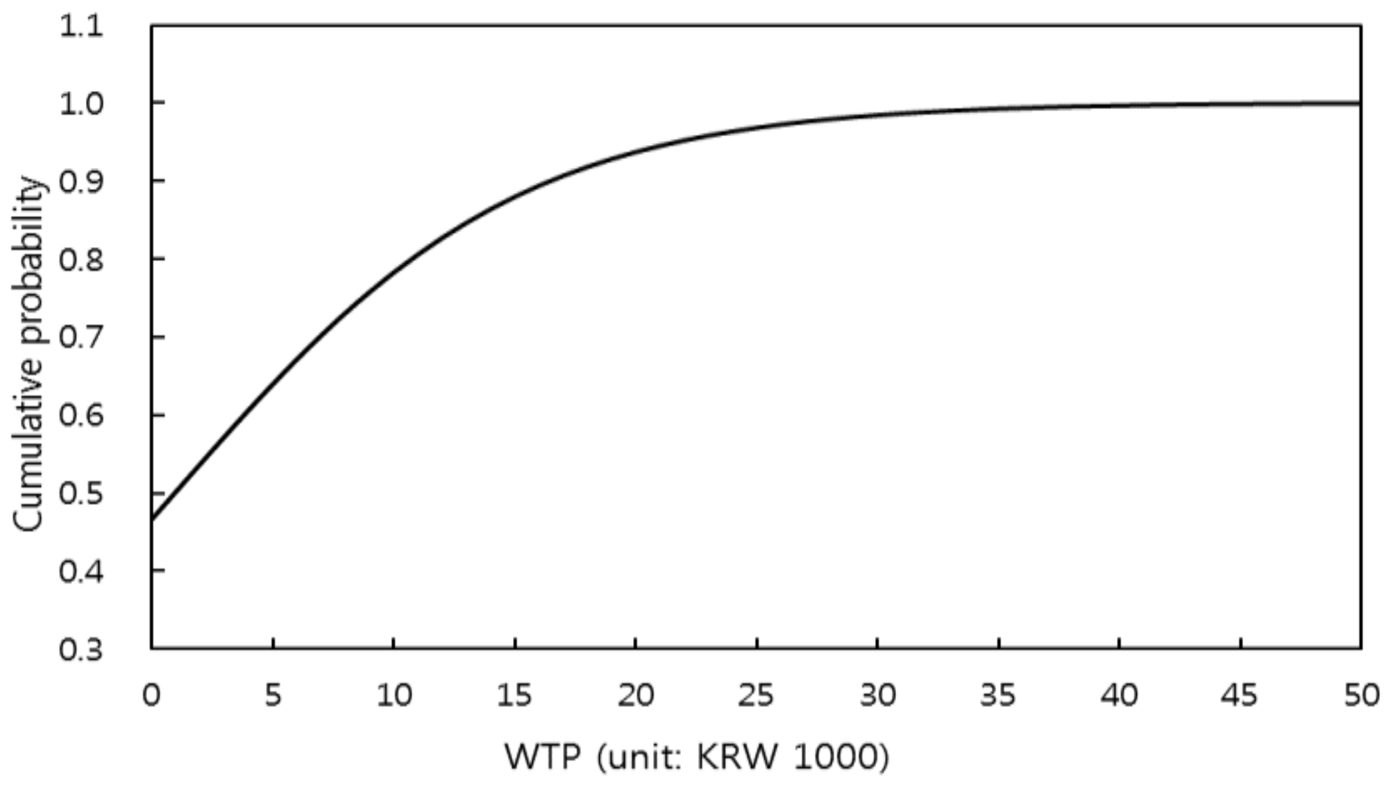
Covariates mean the factors that can make an effect on the likelihood of saying “yes” to a provided bid. Usually, the interviewees’ characteristics are used as covariates. We consider four variables: gender, household size, education level, and income. The variables are explained in Table 1. The covariates are reflected in the model by inserting them into in Equation (1). Therefore, the positive sign of the coefficient for a variable implies that the bigger the value of the variable the higher the probability of saying “yes” to an offered bid. Table 4 denotes the estimation results of the model with covariates. Figure 1 shows the estimated distribution of the WTP with average values for the covariates, via Equation (1).
The coefficient estimates for constant and bid amount terms are statistically significant. More importantly, the estimated coefficient for bid amount variable is negative as expected. The coefficient estimates for Education and Income variables are statistically meaningful, but those for Gender and Family variables are not. The respondent’s education level is positively related to the likelihood of reporting “yes” to a given bid. Similarly, wealthier interviewees are more likely to accept the payment of a proposed bid than less rich interviewees.
We also present the mean WTP estimate from the model with covariates and its 95% confidence interval in Table 4. How much does the WTP change when considering the covariates, even if not significant at the 10% level, provides more details about policies and in particular for informing the population about policy measures as they can be more targeted towards different societal groups. The mean WTP was obtained as KRW 5380 (USD 4.78) and its 95% confidence interval was estimated as KRW 4808 to 6002. To check whether the mean WTP estimate from the model without the covariates is different from that from the model with the covariates, we apply a simple test. The null hypothesis is that they do not differ. Given that the 95% confidence interval from the model with no covariates is KRW 5004 to 6304, the 95% confidence intervals for the mean WTP estimates from the models with the covariates and without the covariates do overlap. Thus, the null hypothesis cannot be rejected at the 5% level, which implies that they do not significantly differ.
4.4. Discussion of the Results
It is necessary to expand the finding for the sample to that for the population. When the survey was conducted, South Korean urban areas had 17,692,275 households [35]. However, the number of observations used here is just one thousand. Therefore, the representativeness of our sample should be examined. That is, whether our sample represents the population well is the key to obtaining information for the population. This study investigates the issue in two aspects before the expansion is performed. First, random and scientific sampling in gathering the data is quite important to the expansion. As explained above, a professional survey company that has rich experience of field CV surveys commissioned the entire process of the sampling, thereby guaranteeing that the sample maintains the representative nature.
Second, whether some variables for the sample are similar to those for the population should be examined. In this regard, the ratio of female respondents, the household’s monthly income, and the size of the household are looked into here. The sample averages for the variables were 50.0%, KRW 4.40 million, and 3.31 persons. The population averages were 50.0%, KRW 4.38 million, 3.09 persons when the survey was conducted [35]. Interestingly, it seems that there are no significant gaps between the two values for each variable. This finding makes the representativeness of our sample even stronger. Thus, the findings from the sample can be expanded to the inference of the population values.
The way in which the covariates are selected may affect the mean WTP estimate. Thus, the mean WTP estimate found in the model with no covariates is used in expanding the sample figure to the population figure instead of that in the model with covariates. When the yearly value concerning the first and the total number of households in urban areas are used, we can compute the total WTP, expanded to the relevant population. As shown in Table 5, it is found that the population’s WTP for reducing the number of the PM2.5 warning issued by half before 2022 in South Korean urban areas is KRW 98.9 billion (USD 87.8 million) per annum. The 95% confidence interval for the total public value is KRW 88.5 to 111.5 billion (USD 78.6 to 99.1 million). It appears that enforcing the PM2.5 concentration reduction policy contributes to South Korean urban area households’ utility.
5. Conclusions
In South Korea, as the PM2.5 concentration in urban areas has increased recently, there is concern about damage to the health of the people. For the purpose of maintaining good public health in urban areas, we should control the concentration of PM2.5, keeping it under a certain level. The South Korean government, therefore, has made a policy of reducing the number of the PM2.5 warnings issued by 50% before 2022 in urban areas. This study applies a CV technique to assess the public value of enforcing the policy. The estimate for the mean annual WTP for the enforcement is KRW 5591 (USD 4.97) per household. It has statistical meaningfulness at the 1% level and the sample also represented the population well. Expanding the value to the whole urban areas of the country results in KRW 98.9 billion (USD 87.8 million) per year.
This article contributes to the existing literature by deriving the household WTP for enforcing the PM2.5 concentration reduction policy in South Korean urban area and evaluating the public value of the enforcement. The study provides empirical evidence that the CV approach theoretically grounded in microeconomics could be successfully utilized in measuring the national public value of the implementation. The authors think that the framework of the study can provide important insights for policy. Currently, government officials are seeking information about the public value of enforcing the policy because the Korean public will pay for the enforcement through national taxes. The results of this study indicate that the public is willing to shoulder some financial burden to enforce the policy.
The authors think that the framework of the study can be extended in future studies in several ways. For example, the cost–benefit analysis (CBA) of the enforcement can provide policy-makers with insights into whether the enforcement is socially profitable. The public value reported above indicates the benefits that ensue from enforcing the PM2.5 concentration policy, which can be used in conventional CBA. Unfortunately, there is no available information about the costs involved in the enforcement. Thus, we refrain from conducting the CBA. As a second stage of this study, the measurement of the costs and the implementation of the CBA should be done in the near future.
Furthermore, the factors affecting the public trust in the policy need to be identified and investigated [41,42]. This is because, if people do not have trust in the policy enforcement, it cannot succeed. Thus, the government should consider which factors are influential and how much the factors affect people’s trust when designing the reduction policy. It may be useful to examine how the public value varies as time passes by conducting the CV survey every year for some years and analyzing the CV data. Investigating how much the public value changes across the regions and identifying other geographic factors which affect the value are also a good research topic. Comparing the findings from this study with those from other studies for foreign countries and analyzing the gap between the two enable us to obtain a new insight into the WTP estimate. These works can provide us with a new point of view concerning the public value.
Acknowledgments
This work was supported by the Korea Institute of Energy Technology Evaluation and Planning (KETEP) and the Ministry of Trade, Industry & Energy (MOTIE) of the Republic of Korea (No. 20164030201060).
Author Contributions
All authors played an important role in the preparation of this paper. Ju-Hee Kim wrote most of the paper; Hyo-Jin Kim conducted the empirical analysis; and Seung-Hoon Yoo took charge of making the survey questionnaire and gathering the data.
Conflicts of Interest
The authors declare no conflict of interest.
Appendix A. Main Part of the Survey Questionnaire
Part 1. Questions about socio-economic characteristics
The interviewees were asked to respond to their socio-economic characteristic such as the gender of the individual, the number of family members, the level of education, and the monthly income per household (before tax deduction). Questions about the number of family and income were open-ended questions, and the question about the level of education was as follows:
Q1. Please check with √ your education level in years.
| Education level | Uneducated | Elementary school | Middle school | High school | University | Graduate school |
| Education level in years | 0 | 1 2 3 4 5 6 | 7 8 9 | 10 11 12 | 13 14 15 16 | 17 18 19 20 |
Part 2. Questions about willingness to pay for reducing the PM2.5 concentration
Type A. Q1. Is your household willing to pay additional income tax of 1000 Korean won (lower bid amount) in annual for the next ten years for enforcing the PM2.5 concentration reduction policy in South Korea, supposing that the project is certain to succeed?
- a.
- Yes—go to Type A. Q2.
- b.
- No—go to Q3.
Type A. Q2. Is your household willing to pay additional income tax of about 3000 Korean won (upper bid amount) in annual for the next ten years for enforcing the PM2.5 concentration reduction policy in South Korea, supposing that the project is certain to succeed?
- a.
- Yes—Finish this survey
- b.
- No—Finish this survey
Type B. Q1. Is your household willing to pay additional income tax of about 3000 Korean won (upper bid amount) in annual for the next ten years for enforcing the PM2.5 concentration reduction policy in South Korea, supposing that the project is certain to succeed?
- a.
- Yes—Finish this survey
- b.
- No—go to Type B. Q2.
Type B. Q2. Is your household willing to pay additional income tax of about 1000 Korean won (lower bid amount) in annual for the next ten years for enforcing the PM2.5 concentration reduction policy in South Korea, supposing that the project is certain to succeed?
- a.
- Yes—Finish this survey
- b.
- No—go to Q3.
Q3. Then, is your household not willing to pay anything for enforcing the PM2.5 concentration reduction policy in South Korea?
- a.
- Yes, our household is willing to pay something less than 1000 Korean won.
- b.
- No, our household is not willing to pay anything. In other words, our household’s willingness to pay is zero.
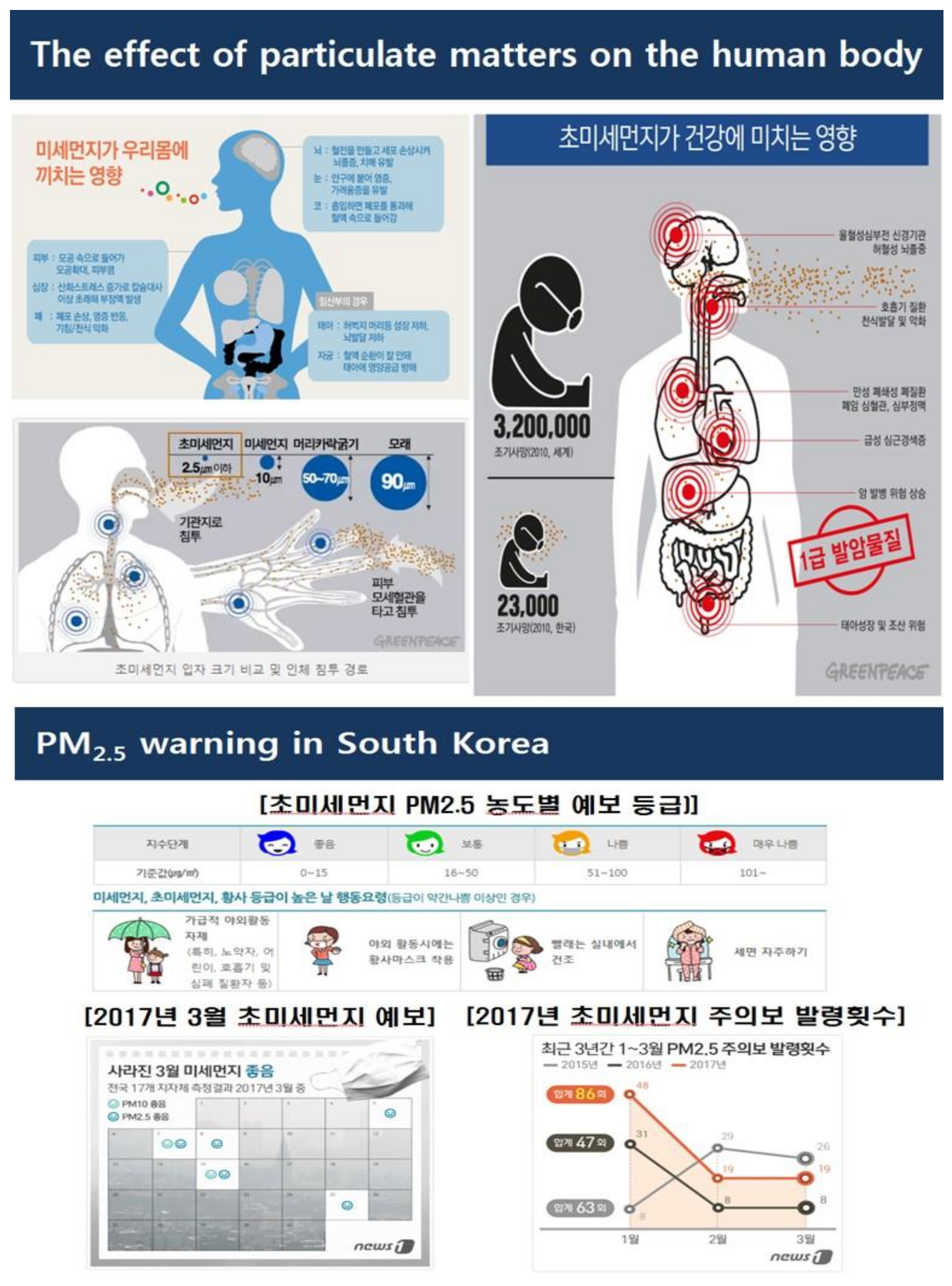
Figure A1.
Information materials used to inform interviewees about the issues of PM2.5 in Korean.

References
- World Health Organization. 7 Million Premature Deaths Annually Linked to Air Pollution. 2014. Available online: http://www.who.int/mediacentre/news/releases/2014/air-pollution/en (accessed on 20 October 2017).
- International Agency for Research on Cancer. Outdoor Air Pollution a Leading Environmental Cause of Cancer Deaths; World Health Organization: Geneva, Switzerland, 2013. [Google Scholar]
- Laden, F.; Neas, L.M.; Dockery, D.W.; Schwartz, J. Association of fine particulate matter from different sources with daily mortality in six U.S. cities. Environ. Health Perspect. 2000, 108, 941–947. [Google Scholar] [CrossRef] [PubMed]
- Zíková, N.; Wang, Y.; Yang, F.; Li, X.; Tian, M.; Hopke, P.K. On the source contribution to Beijing PM2.5 concentrations. Atmos. Environ. 2016, 134, 84–95. [Google Scholar] [CrossRef]
- Maynard, R.L.; Howard, V. Particulate Matter: Properties and Effects upon Health; Bios Scientific Pub Limited: Oxford, UK, 1999. [Google Scholar]
- Harrison, R.M.; Yin, J. Particulate matter in the atmosphere: Which particle properties are important for its effects on health? Sci. Total Environ. 2000, 249, 85–101. [Google Scholar] [CrossRef]
- Shaughnessy, W.J.; Venigalla, M.M.; Trump, D. Health effects of ambient levels of respirable particulate matter (PM) on healthy, young-adult population. Atmos. Environ. 2015, 123, 102–111. [Google Scholar] [CrossRef]
- Xing, Y.F.; Xu, Y.H.; Shi, M.H.; Lian, Y.X. The impact of PM2.5 on the human respiratory system. J. Thorac. Dis. 2016, 8, 69–74. [Google Scholar]
- Dominici, F.; Peng, R.D.; Bell, M.L.; Pham, L.; McDermott, A.; Zeger, S.L.; Samet, J.M. Fine particulate air pollution and hospital admission for cardiovascular and respiratory diseases. J. Am. Med. Assoc. 2006, 295, 1127–1134. [Google Scholar] [CrossRef] [PubMed]
- Zanobetti, A.; Franklin, M.; Koutrakis, P.; Schwartz, J. Fine particulate air pollution and its components in association with cause-specific emergency admissions. Environ. Health 2009, 8, 58. [Google Scholar] [CrossRef] [PubMed]
- Achillas, C.; Vlachokostas, C.; Moussiopoulos, Ν.; Banias, G. Prioritize strategies to confront environmental deterioration in urban areas: Multicriteria assessment of public opinion and experts’ views. Cities 2011, 28, 414–423. [Google Scholar] [CrossRef]
- Kim, H.K.; Kang, K.M.; Kim, T.Y. Measurement of particulate matter (PM2.5) and health risk assessment of cooking-generated particles in the kitchen and living rooms of apartment houses. Sustainability 2018, 10, 843. [Google Scholar] [CrossRef]
- Wong, L.P.; Alias, H.; Aghamohammadi, N.; Ghadimi, A.; Sulaiman, N.M.N. Control measures and health effects of air pollution: A survey among public transportation commuters in Malaysia. Sustainability 2017, 9, 1616. [Google Scholar] [CrossRef]
- Nguyen, T.N.; Park, D.; Lee, Y.; Lee, Y.C. Particulate matter (PM10 and PM2.5) in subway systems: Health-based economic assessment. Sustainability 2017, 9, 2135. [Google Scholar] [CrossRef]
- Harris, B.; Kang, B.S. South Korea Joins Ranks of WORLD’S most Polluted Countries. Financial Times. 2017. Available online: https://www.ft.com/content/b49a9878-141b-11e7-80f4-13e067d5072c (accessed on 20 October 2017).
- Organization for Economic Co-operation and Development. Exposure to PM2.5 in Countries and Regions. 2017. Available online: http://stats.oecd.org/index.aspx?queryid=72722 (accessed on 20 October 2017).
- Korea Ministry of Environment. Monthly Report of Air Quality. 2015. Available online: http://www.me.go.kr (accessed on 20 October 2017).
- Korea Ministry of Environment. Monthly Report of Air Quality. 2016. Available online: http://www.me.go.kr (accessed on 20 October 2017).
- Korea Ministry of Environment. Monthly Report of Air Quality. 2017. Available online: http://www.me.go.kr (accessed on 20 October 2017).
- The Straits Times. S. Korea Among Most Polluted Nations. 2017. Available online: http://www.straitstimes.com/asia/east-asia/s-korea-among-most-polluted-nations (accessed on 20 October 2017).
- Air Korea. Regional Air Quality. Available online: http://www.airkorea.or.kr/pmRelay?itemCode=11008 (accessed on 20 October 2017).
- Yoo, S.H.; Kwak, S.J.; Lee, J.S. Using a choice experiment to measure the environmental costs of air pollution impacts in Seoul. J. Environ. Manag. 2008, 86, 308–318. [Google Scholar] [CrossRef] [PubMed]
- Park, S.Y.; Lim, S.Y.; Yoo, S.H. The economic value of the national meteorological service in the Korean household sector: A contingent valuation study. Sustainability 2016, 8, 834. [Google Scholar] [CrossRef]
- Netalieva, I.; Wesseler, J.; Heijman, W. Health costs caused by oil extraction air emissions and the benefits from abatement: The case of Kazakhstan. Energy Policy 2005, 33, 1169–1177. [Google Scholar] [CrossRef]
- Wang, Y.; Zhang, Y.S. Air quality assessment by contingent valuation in Ji’nan, China. J. Environ. Manag. 2009, 90, 1022–1029. [Google Scholar] [CrossRef] [PubMed]
- Lee, J.Y.; Lim, Y.W.; Yang, J.Y.; Kim, C.S.; Shin, Y.C.; Shin, D.C. Evaluating the PM damage cost due to urban air pollution and vehicle emissions in Seoul, Korea. J. Environ. Manag. 2011, 92, 603–609. [Google Scholar] [CrossRef] [PubMed]
- EI-Fadel, M.; Massoud, M. Particulate matter in urban areas: Health-based economic assessment. Sci. Total Environ. 2000, 257, 133–146. [Google Scholar] [CrossRef]
- Wang, J.; Wang, S.; Voorhees, A.S.; Zhao, B.; Jang, C.; Jiang, J.; Fu, J.S.; Ding, D.; Zhu, Y.; Hao, J. Assessment of short-term PM2.5-related mortality due to different emission sources in the Yangtze River Delta, China. Atmos. Environ. 2015, 123, 440–448. [Google Scholar] [CrossRef]
- Tang, C.; Zhang, Y. Using discrete choice experiments to value preferences for air quality improvement: The case of curbing haze in urban China. J. Environ. Plan. Manag. 2016, 59, 1473–1494. [Google Scholar] [CrossRef]
- Wei, W.; Yan, W. Willingness to pay to control PM2.5 pollution in Jing-Jin-Ji Region, China. Appl. Econ. Lett. 2017, 24, 753–761. [Google Scholar] [CrossRef]
- Carlsson, F.; Johansson-Stenman, O. Willingness to pay for improved air quality in Sweden. Appl. Econ. 2000, 32, 661–669. [Google Scholar] [CrossRef]
- Cooper, J.C.; Hanemann, W.M.; Signorello, G. One and one-half bound dichotomous choice contingent valuation. Rev. Econ. Stat. 2002, 84, 742–750. [Google Scholar] [CrossRef] [Green Version]
- Kriström, B. Spike model in contingent valuation. Am. J. Agric. Econ. 1997, 79, 1013–1023. [Google Scholar] [CrossRef]
- Arrow, K.; Solow, R.; Portney, P.R.; Leamer, E.E.; Radner, R.; Schuman, H. Report of the NOAA panel on contingent valuation. Fed. Regist. 1993, 58, 4601–4614. [Google Scholar]
- Statistics Korea. Available online: http://kosis.kr (accessed on 20 October 2017).
- Hanemann, W.M. Welfare evaluations in contingent valuation experiments with discrete responses. Am. J. Agric. Econ. 1984, 66, 332–341. [Google Scholar] [CrossRef]
- Champ, P.A.; Boyle, K.J.; Brown, T.C.A. Primer on Nonmarket Valuation; Kluwer Academic Publisher: Dordrecht, The Netherlands, 2004. [Google Scholar]
- Johnston, R.J.; Boyle, K.J.; Adamowicz, W.; Bennett, J.; Brouwer, R.; Cameron, T.A.; Hanemann, W.M.; Hanley, N.; Ryan, M.; Scarpa, R.; et al. Contemporary guidance for stated preference studies. J. Assoc. Environ. Resour. Econ. 2017, 4, 319–405. [Google Scholar] [CrossRef]
- Hanemann, W.M.; Loomis, J.; Kanninen, B.J. Statistical efficiency of double-bounded dichotomous choice contingent valuation. Am. J. Agric. Econ. 1991, 73, 1255–1263. [Google Scholar] [CrossRef]
- Krinsky, I.; Robb, A.L. On approximating the statistical properties of elasticities. Rev. Econ. Stat. 1986, 68, 715–719. [Google Scholar] [CrossRef]
- Kikulwe, E.M.; Wesseler, J.; Falck-Zepeda, J. Attitudes, perceptions, and trust. Insights from a consumer survey regarding genetically modified banana in Uganda. Appetite 2011, 57, 401–413. [Google Scholar] [CrossRef] [PubMed]
- Kikulwe, E.M.; Falck-Zepeda, J.; Wesseler, J. If labels for GM food were present, would consumers trust them?’ Insights from a consumer survey in Uganda. Environ. Dev. Econ. 2013, 19, 786–805. [Google Scholar] [CrossRef]
Figure 1.
Distribution function of the willingness to pay (WTP).


Table 1.
Description of the socio-economic characteristics of the interviewees.
| Variables | Definitions | Mean | Standard Deviation |
|---|---|---|---|
| Gender | The respondent’s gender (0 = male; 1 = female) | 0.50 | 0.50 |
| Family | The size of the respondent’s household (unit: persons) | 3.31 | 1.05 |
| Education | The respondent’s education level in years | 14.23 | 2.28 |
| Income | The household’s monthly income before tax deduction (unit: million Korean) | 4.40 | 2.01 |
Table 2.
Summary of the interviewees’ responses to each set of bids.
| Bid Amount a | Lower Bid Is Offered at First (%) b | Upper Bid Is Offered at First (%) b | Sample Size | |||||||
|---|---|---|---|---|---|---|---|---|---|---|
| “yes–yes” | “yes–no” | “no–yes” | “no–no” | “yes” | “no–yes” | “no–no–yes” | “no–no–no” | |||
| 1000 | 3000 | 27 (18.9) | 19 (13.3) | 3 (2.1) | 23 (16.1) | 31 (21.7) | 12 (8.4) | 1 (0.7) | 27 (18.9) | 143 (100.0) |
| 2000 | 4000 | 21 (14.7) | 16 (11.2) | 12 (8.4) | 22 (15.4) | 27 (18.9) | 3 (2.1) | 7 (4.9) | 35 (24.5) | 143 (100.0) |
| 3000 | 6000 | 16 (11.2) | 13 (9.1) | 16 (11.2) | 26 (18.2) | 28 (19.6) | 6 (4.2) | 6 (4.2) | 32 (22.4) | 143 (100.0) |
| 4000 | 8000 | 12 (8.4) | 13 (9.1) | 11 (7.7) | 36 (25.2) | 19 (13.3) | 8 (5.6) | 10 (7.0) | 34 (23.8) | 143 (100.0) |
| 6000 | 10,000 | 15 (10.6) | 9 (6.3) | 7 (4.9) | 40 (28.2) | 21 (14.8) | 4 (2.8) | 5 (3.5) | 41 (28.9) | 142 (100.0) |
| 8000 | 12,000 | 13 (9.2) | 13 (9.2) | 10 (7.0) | 35 (24.6) | 14 (9.9) | 4 (2.8) | 17 (12.0) | 36 (25.4) | 142 (100.0) |
| 10,000 | 15,000 | 15 (10.4) | 9 (6.3) | 8 (5.6) | 40 (27.8) | 17 (11.8) | 3 (2.1) | 14 (9.7) | 38 (26.4) | 144 (100.0) |
| Sample size | 119 (11.9) | 92 (9.2) | 67 (6.7) | 222 (22.2) | 157 (15.7) | 40 (4.0) | 60 (6.0) | 243 (24.3) | 1000 (100.0) | |
Notes: a The unit is Korean won (USD 1.0 = KRW 1126 at the time of the survey). b The percentage of sample size is given in parentheses beside the number of responses.
Table 3.
Estimation results of the model.
| Variables | Estimates d |
|---|---|
| Constant | 0.1146 (1.84) * |
| Bid amount a | −0.1345 (−17.95) # |
| Spike | 0.4714 (30.31) # |
| Yearly mean WTP per household t-value 95% confidence interval b | KRW 5591 (USD 4.97) 17.13 # KRW 5004 to 6304 (USD 4.44 to 5.60) |
| Sample size | 1000 |
| Log-likelihood | −1259.67 |
| Wald statistic (p-value) c | 293.48 (0.000) |
Notes: a The unit is KRW 1000, and the exchange rate was USD 1.0 = KRW 1126 at the time of the survey. b It is calculated using the parametric bootstrapping method given in Krinsky and Robb [40]. c It is computed under the null hypothesis of all the parameters’ being jointly zero. d The values reported in parentheses beside the coefficient estimates are t-values. # and * imply statistical meaningfulness at the 1% and 10% levels, respectively.
Table 4.
Estimation results of the model with covariates.
| Variables a | Estimates | t-values |
|---|---|---|
| Constant | −2.3946 | −5.66 # |
| Bid amount b | −0.1412 | −18.01 # |
| Gender | 0.1037 | 0.85 |
| Family | −0.0662 | −1.03 |
| Education | 0.1568 | 5.44 # |
| Income | 0.1044 | 3.05 # |
| Spike | 0.4679 | 29.47 # |
| Yearly mean WTP per household t-value 95% confidence interval c | KRW 5380 (USD 4.78) 17.30 # KRW 4808 to 6022 (USD 4.27 to 5.35) | |
| Wald statistic (p-value) d | 299.33 (0.000) | |
| Log-likelihood | −1232.10 | |
| Number of observations | 1000 | |
Notes: a Table 1 explains the variables. b The unit is KRW 1000 (USD 1.0 = KRW 1126 at the time of the survey). c It is calculated using the parametric bootstrapping method given in Krinsky and Robb [40]. d It is computed under the null hypothesis of all the parameters’ being jointly zero. # implies statistical meaningfulness at the 1% level.
Table 5.
Estimation of total willingness to pay (WTP).
| Estimates | 95% Confidence Intervals | |
|---|---|---|
| Mean annual WTP per household | KRW 5591 (USD 4.97) | KRW 5004 to 6304 (USD 4.44 to 5.60) |
| Total annual WTP | KRW 98.9 billion (USD 87.8 million) | KRW 88.5 to 111.5 billion (USD 78.6 to 99.1 million) |
Note: South Korean urban areas had 17,692,725 households at the time of the survey.
© 2018 by the authors. Licensee MDPI, Basel, Switzerland. This article is an open access article distributed under the terms and conditions of the Creative Commons Attribution (CC BY) license (http://creativecommons.org/licenses/by/4.0/).
Share and Cite
MDPI and ACS Style
Kim, J.-H.; Kim, H.-J.; Yoo, S.-H. Public Value of Enforcing the PM2.5 Concentration Reduction Policy in South Korean Urban Areas. Sustainability 2018, 10, 1144. https://doi.org/10.3390/su10041144
AMA Style
Kim J-H, Kim H-J, Yoo S-H. Public Value of Enforcing the PM2.5 Concentration Reduction Policy in South Korean Urban Areas. Sustainability. 2018; 10(4):1144. https://doi.org/10.3390/su10041144
Chicago/Turabian StyleKim, Ju-Hee, Hyo-Jin Kim, and Seung-Hoon Yoo. 2018. "Public Value of Enforcing the PM2.5 Concentration Reduction Policy in South Korean Urban Areas" Sustainability 10, no. 4: 1144. https://doi.org/10.3390/su10041144
Note that from the first issue of 2016, this journal uses article numbers instead of page numbers. See further details here.