Role of Scirpus mariqueter on Methane Emission from an Intertidal Saltmarsh of Yangtze Estuary
by
 ,
,
Yangjie Li
1,2, 
Dongqi Wang
2,*,
Zhenlou Chen
2,
Haiyan Jin
1,
Hong Hu
2,
Jianfang Chen
1 and
Zhi Yang
1 1
Key Laboratory of Marine Ecosystem and Biogeochemistry of State Ocean Administration, Second Institute of Oceanography, State Ocean Administration, Hangzhou 310012, China
2
School of Geographic Sciences, East China Normal University, Shanghai 200241, China
*
Author to whom correspondence should be addressed.
Sustainability 2018, 10(4), 1139; https://doi.org/10.3390/su10041139
Submission received: 25 December 2017
/
Revised: 4 April 2018
/
Accepted: 4 April 2018
/
Published: 10 April 2018
(This article belongs to the Special Issue Marine Carbon Cycles)
Abstract
:The role of wetland plant (Scirpus mariqueter) on methane (CH4) emissions from a subtropical tidal saltmarsh of Yangtze estuary was investigated over a year. Monthly CH4 flux and pore-water CH4 concentration were characterized using static closed chamber technique and pore-water extraction. Measured chamber CH4 fluxes indicated that saltmarsh of the Yangtze estuary acted as a net source of atmospheric CH4 with annual average flux of 24.0 mgCH4·m−2·day−1. The maximum chamber CH4 flux was in August (91.2 mgCH4·m−2·day−1), whereas the minimum was observed in March (2.30 mgCH4·m−2·day−1). Calculated diffusion CH4 fluxes were generally less than 6% of the chamber fluxes. Significant correlations were observed between the chamber CH4 flux and rhizospheric pore-water CH4 concentration (11–15 cm: p < 0.05, R = 0.732; 16–20 cm: p < 0.05, R = 0.777). In addition, chamber CH4 fluxes from July to September constituted more than 80% of the total annual emission and were closely correlated with aboveground biomass yield of S. mariqueter. The results indicated that S. mariqueter transportation was the dominant CH4 emission pathway and it provided an efficient route for the belowground CH4 to escape into the atmosphere while avoiding oxidation, leading to CH4 emissions.
1. Introduction
Methane (CH4) is the second most important greenhouse gas in the atmosphere [1]. One of important pathways of CH4 formation is through fermentation mediated by microbiological process and controlled by oxygen availability and the amount of labile organic matter [2]. Another CH4 formation pathway is carbonate reduction, which is believed to be a main process of CH4 production in marine systems [3]. As CH4 exchange at air–soil boundary layer is determined by its net result of production and consumption, CH4 emissions at ecosystem level cannot be accurately quantified without accounting for the potential of CH4 oxidation [4,5,6]. It has been reported that most of the CH4 formed in the anoxic environment is biologically oxidized to CO2 before escaping out of the sediments [7,8]. In wetland sediments, CH4 oxidation mediated by methanotrophs could occur in both aerobic and anaerobic conditions [9,10,11].
There are three pathways for dissolved CH4 in sediment pore-water to reach the atmosphere: molecular diffusion, bubble ebullition, and vascular plant transport [12,13]. High belowground CH4 stock resulted from rapid microbial CH4 production creates concentration gradients at air–soil boundary layers [14], which drives CH4 diffusion following the Fick’s first law [15]. In some cases, the diffusion fluxes were found to be smaller than bubble ebullition and vascular plants transport [16]. To adapt to long-term water flooding, wetland plants develop aerenchyma as a pathway for internal gas transport. This pathway is bidirectional such that oxygen can be transported belowground tissues and CH4 be vented to the atmosphere [17]. Wetland plants can also greatly influence CH4 production and consumption by secreting O2 and exudates in rhizosphere [18,19,20]. In addition, the plant transportation of CH4 could play an important role in CH4 emissions [14]. This is especially true in vegetated wetlands where plant transportation usually acts as the main emission pattern of CH4 [20,21], even though the magnitude of CH4 emissions may vary significantly among different species [20,22,23,24].
The Yangtze estuary, located in the subtropical area with a clear four seasons, is one of the biggest estuaries in the world. Annually, the Yangtze River transports 4.80 × 10⁸ tons of sediment to the East China Sea, and about half of that settles in the estuary, thereby forming an extensive intertidal zone [25]. Thus, intertidal marshes in Yangtze estuary may play an important role in carbon cycles including both carbon sequestration and release in the regional scale. Previously, Wang et al. [26] reported the CH4 emission fluxes and seasonal influence in this area. Bu et al. [27] studied the semi-lunar tidal cycling on sediment CH4 emissions. Yin et al. [28] revealed the influences of Spartina alterniflora invasions on both CH4 and N2O fluxes from the salt marsh, just north of Yangtze estuary. However, few studies focused on the influence of the endemic plant (S. mariqueter) on CH4 emissions in Yangtze estuary. Clarification of the relative contribution of two emission pathways, molecular diffusion and plant transport, would be very useful to reveal the plants’ contribution to CH4 emissions. Besides, Yangtze estuary is also faced with the invasion of the exotic Spartina alterniflora, which could greatly decrease the plant density of S. mariqueter, thus changing the CH4 emissions. Therefore, the objectives of this case study were: (1) to elucidate the role of S. mariqueter on methane emission; (2) to identify the seasonal CH4 emission patterns; and (3) to examine the relationship between CH4 emissions and pore-water CH4 concentrations, at representative point of an intertidal saltmarsh at Yangtze estuary.
2. Methods and Materials
2.1. Study Site
Yangtze estuarine wetlands continue extending to East China Sea rapidly because of the abundant sediment import from the upper reaches [25]. Dongtan in the east Chongming Island is the largest and most conserved intertidal wetland in Yangtze estuary, which is about 100 km2 and composed of saltmarsh and bare flat. The shape of saltmarsh is semilunar, and the widest middle part is about 4 km (Figure 1). Research and sampling point is selected at about the center of the saltmarsh (31°30.111′ N, 121°59.024′ E). The point is not submerged during the neap tide and submerged for several hours during the spring tide. Sampling was carried out at low tide. Phragmites, S. mariqueter and the invasive Spartina alterniflora compose the vegetation community of saltmarshes. S. mariqueter is the native species in Yangtze estuary. In general, one axillary bud per corm sprouts to form a new shoot at the depth of 20 cm in spring, which determines that most of the roots distribute within the depth of 20 cm [29]. At the base of the new shoot, constituted by a corm, usually one to three rhizomes develop and form new shoots [30]. The growing season for S. mariqueter generally occurs from late April to early November with the most active growth occurring during the three summer months (July, August and September), and it dies off at the end of the growing season and they gradually fall over. Along with the continuous sediment deposition, the dead plant will be buried by the sediment and they cannot be flow out with the tide due to the deeper root fixation [31].
2.2. Sampling
A sediment core (60-cm long) was collected monthly from April to December 2011 using a PVC pipe (inner diameter: 12 cm, length: 100 cm). Core sampling was not carried out from January to March because the preparatory work was not being done during that period. The core was sealed with tapes and carried back to the laboratory for the measurement of pore-water CH4 concentration within one day.
Static closed chamber technique was adopted to measure CH4 fluxes 70 times from February to December 2011. Three stainless-steel collars were inserted into the soil to a depth of 5 cm including one bunch of moderate growth size of Scirpus mariqueter, half hour before gas sampling, and, then, triplicate transparent chambers made of 3-mm thickness Perspex cylinder were placed on collars, and an airtight closure was ensured by water sealing during the measurements. Considering that the vegetation height, even during the peak of the growing season, was no more than 50 cm, the dimensions of the chambers are 50-cm height and 30-cm inner diameter. Small electric fans and kerosene thermometers were fixed inside the chambers for the air blending in the chambers and the temperature measurement inside the chambers. For each chamber, a venting tube (5 mm inner diameter and 18.8 m long) was used to balance the air pressure between inside and outside chambers [32], and a polyethylene pipe connected with a three-way stopcock was fixed on the chamber top for sampling. All the connections and gaps were sealed by silicone gel to ensure chambers were air tight. Immediately after installing each chamber and again 30 min later, 180 mL gas sample was drawn out by using a syringe with a three-way airtight stopcock and injected into a pre-vacuumed air bag (plastic bag plated with Aluminum inside), which is inert to the greenhouse gas. Gas samples were carried back to the laboratory and analyzed for CH4.
Environmental factors including light intensity, air temperature and sediment temperature at different depths (5 cm, 10 cm and 15 cm) were recorded synchronously using a TES-1332 photometer, spirit thermometer and geothermometer at each time of gas sampling. The aboveground biomass of S. mariqueter was measured monthly from April to December. Vegetation samples were collected from seven 50 cm × 50 cm randomly selected quadrats, maintaining approximately 3–5 m spacing between quadrats. In each quadrat, the aboveground vegetation was cut carefully, then the number of living shoots were counted, and the shoot weight and cross-section area were measured and recorded.
2.3. Pore-Water CH4 Extraction
The pore-water CH4 concentration was measured in the laboratory based on static headspace method within one day after the core was sampled. Fifty milliliters of distilled water were transported into a headspace tube equipped with a screws cap which has a hole and silicone septum. The 60-cm long sediment cores were sliced at 1-cm interval, and then 10 mL of the subsamples in each layer were put into the prepared headspace tube quickly. The tube was capped with the silicone septum immediately and set on a shaker for 20 min at 150 rpm to make the sediment fully blend with the aerated distilled water forming slurry and gas equilibrium between slurry and headspace air. After 20 min of shaking, 10 mL gas sample was extracted with a 50 mL syringe from the headspace of each tube for CH4 concentration measurement.
2.4. Sediment Properties
The CH4 in samples was measured using an Agilent 7890A Gas Chromatography (GC) equipped with a FID detector. Sediment water content was calculated based on the mass method. The wet and dry weight of the sediment samples were separately measured before and after they were freeze-dried with a freeze dryer (CHRIST ALPHA 4-1/LD plus). Dried sediment samples were ground and sieved to analyze sediment organic carbon (SOC) based on K2Cr2O7-H2SO4 oxidation method [33]. The sediment water content (SWC) was obtained by using the difference between the wet and dry weights. Average particle size (APS) and medium diameter (MD) are measured by laser granularity meter (Coulter LS13320). Extractable nitrogen (NO3−-N and NH4+-N) was determined by extracting 10 g of dry sediment sample with 2 mol·L−1 KCl followed by detection of NO3−N using a continuous flow analyzer (FUTURA, Alliance Co.), and NH4+-N based on standard colorimetric method [34]. For acid volatile sulfide (AVS) measurement, approximately 2 g of sediment were added to the reaction flask and sparged for 2 min with pure N2 (120 cm3·min−1). The sulfide in the sediment was liberated by extraction with 1 mol·L−1 HCl for 40 min at room temperature and then trapped in a solution of 0.2 mol·L−1 (CH3COO)2Zn and 0.1 mol·L−1 CH3COONa with a continuous N2 flow to form ZnS. Each trap was quantified using the methylene blue method [35,36].
2.5. Data Calculating
Chamber flux was calculated based on the following equation:
FistheCH4 fluxes at the sediment–air interface (mgCH4·m−2·h−1), V is the chamber volume(m3), A is the sediment area in the base of sampling chamber(m2), is the change of CH4 concentration with time (mgCH4·L−1·h−1), (mgCH4·L−1), P is the atmospheric pressure in sampling field, R is the gas constant (8.314 J·mol−1·K−1), T is the temperature (Kelvin Temperature, K), and m is the molar mass of the gas molecule.
Pore-water CH4 concentration was calculated by the following equation:
C is the CH4 concentration in pore-water (mgCH4·L−1), CAIR is the measured CH4 concentration in the headspace of tubes (mgCH4·L−1), VAIR is the volume of the headspace of tubes (L), and is the Bunsen coefficient. VWATER is the total volume of aerated distilled water in tubes and the pore water in sediment samples (L). VPOREWATER is the volume of the pore water of the sediment sample (L). CBLANK is the measured CH4 concentration of the pure water (mgCH4·L−1).
Diffusive fluxes of CH4 were calculated from linear pore-water concentration gradients according to Fick’s first law assuming steady state conditions. The diffusion equation is described as Equation (3):
where is the calculated diffusion CH4 flux (μmolCH4·cm−2·s−1), represents the CH4 concentration change with sediment depth (μmolCH4·cm−3·cm−1), ΔZ is the diffusion distance (cm), CS is measured CH4 concentration in the surface sediment pore water (μmolCH4·cm−3), CA is the saturation concentration of dissolved CH4 in ambient air (μmolCH4·cm−3), and Ds is the effective diffusion coefficient for CH4 in sediment pore-water. Ds is calculated by the polynomial regression equation obtained by the measured diffusion coefficients for CH4 in water (Dw) in the range 0 °C to 35 °C (cm2·s−1) (83rd Edition of the Handbook of Physics and Chemistry) which yielded the relationship [37]:
and then porosity corrected by Equation (5) from Lerman [38]:
where φ is sediment porosity. To make the calculated diffusion flux be consistent with the total emission flux, was finally expressed in mgCH4·m−2·day−1.
Dw = 8.889 × 10⁻¹¹T3 − 1.714 × 10⁻⁹T2 + 3.721 × 10⁻⁷T + 8.771 × 10⁻⁶
Ds = Dw × φ2
2.6. Statistical Analysis
The total CH4 fluxes were presented as means of the replications. SPSS (Version 17.0) was used to perform all of the statistical data tests. Pearson correlation analyses were used to examine the relationship between fluxes and the measured environmental variables. The statistical results were regarded as significant if the P values were lower than 0.05 or 0.01.
3. Results
3.1. Environmental Factors
Table 1 shows seasonal climatic, vegetation and soil physiochemical parameters of experimental site. Air temperature exhibited significant seasonal variation with the highest and lowest temperatures in July and February, respectively. Highest biomass of S. mariqueter occurred in August (692.6 g·m−2). The number of living shoots increased with the biomass and also reached the highest value in August. Since then, the plant began to wither and almost all of them fell over on the sediment surface in December. SOC did not show substantial changes throughout the year. SWC stayed at a relatively low level from February to April but increased in the following months. APS and MD indicated that sediment was dominated by silt fractions. In terms of the extractable nitrogen, NH4+-N content was generally higher than that of NO3−-N, which probably indicated that the tidal marsh was generally under denitrification condition rather than nitrification. On the other hand, the irregular variation of AVS content throughout the year suggested that the redox potential of the microenvironment may differ a lot in this estuarine system (Table 1). AVS is mainly produced by the sulfate reduction process which occurred after the O2 and NO3− were utilized. Thus, AVS can be seen as an index of the sediment redox condition. Monthly AVS distribution in the sediment profile is shown in Figure 2, which indicated that the AVS in the surface sediment is usually lower than the deeper sediment. Besides, the AVS showed complex variation along with depth and month.
3.2. CH4 Fluxes
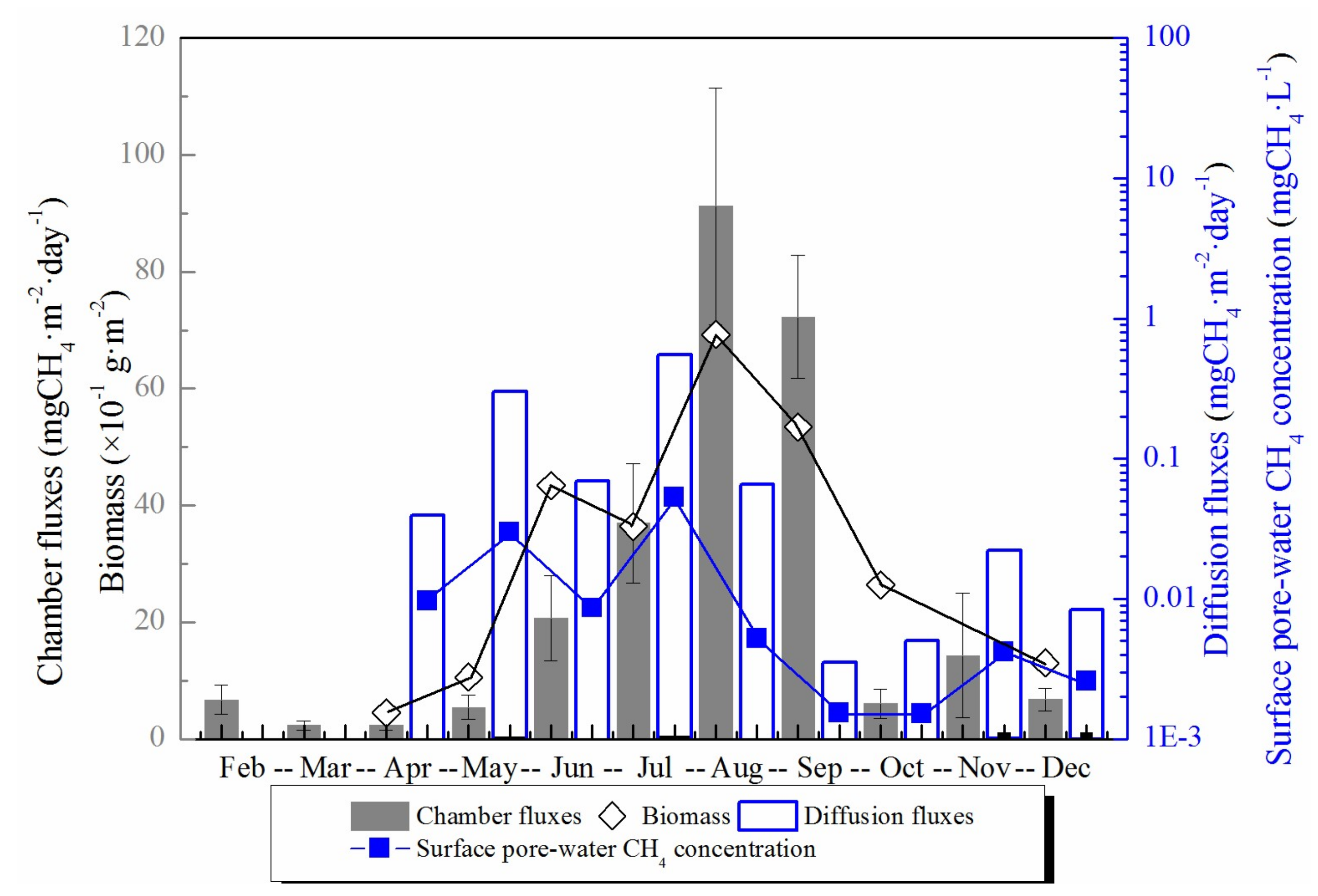
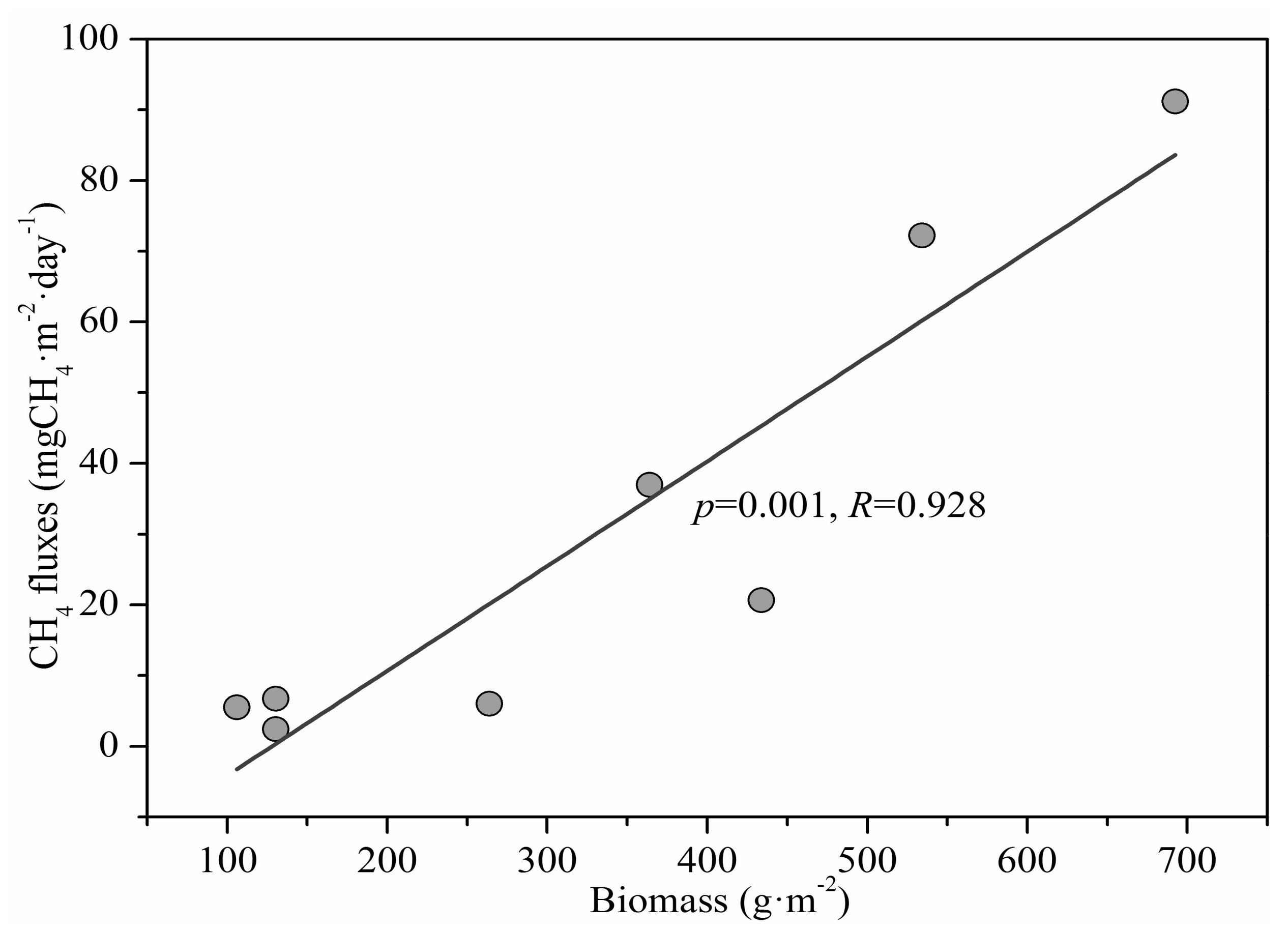
Measured chamber CH4 fluxes showed a significant seasonal variation throughout the year with the highest (91.2 mgCH4·m−2·day−1) and lowest (2.30 mgCH4·m−2·day−1) in August and March, respectively (Figure 3). The annual average chamber CH4 flux in the salt marsh was 24.0 mgCH4·m−2·day−1. The chamber CH4 flux did not increase significantly until June when the biomass of S. mariqueter rather than temperature increased significantly, and the chamber CH4 flux was significantly positively correlated with the aboveground biomass (p = 0.001, R = 0.928) (Figure 4). Chamber CH4 flux during summer (July, August and September) constituted more than 80% of the total annual emission.
Calculated diffusion CH4 fluxes between the top 1 cm sediment and air were very low (<0.55 mgCH4·m−2·day−1) due to the low pore-water CH4 concentration in surface sediment (Figure 3). There was evident seasonal variation of diffusion CH4 fluxes with the highest (0.55 mgCH4·m−2·day−1) and lowest (0.0035 mgCH4·m−2·day−1) diffusion flux in July and September, respectively (Figure 3). Overall, gas molecular diffusion method contributed a little to the total CH4 emission with the highest proportion of 5.53% in May.
In addition, regression analysis of different temperatures (air temperature and the sediment temperature at different depths 5 cm, 10 cm and 15 cm) and chamber CH4 fluxes revealed that CH4 fluxes were best fitted with the temperature at the sediment depth of 15 cm where the roots of S. mariqueter were concentrated (Figure 5).
3.3. Pore-Water CH4 Concentration
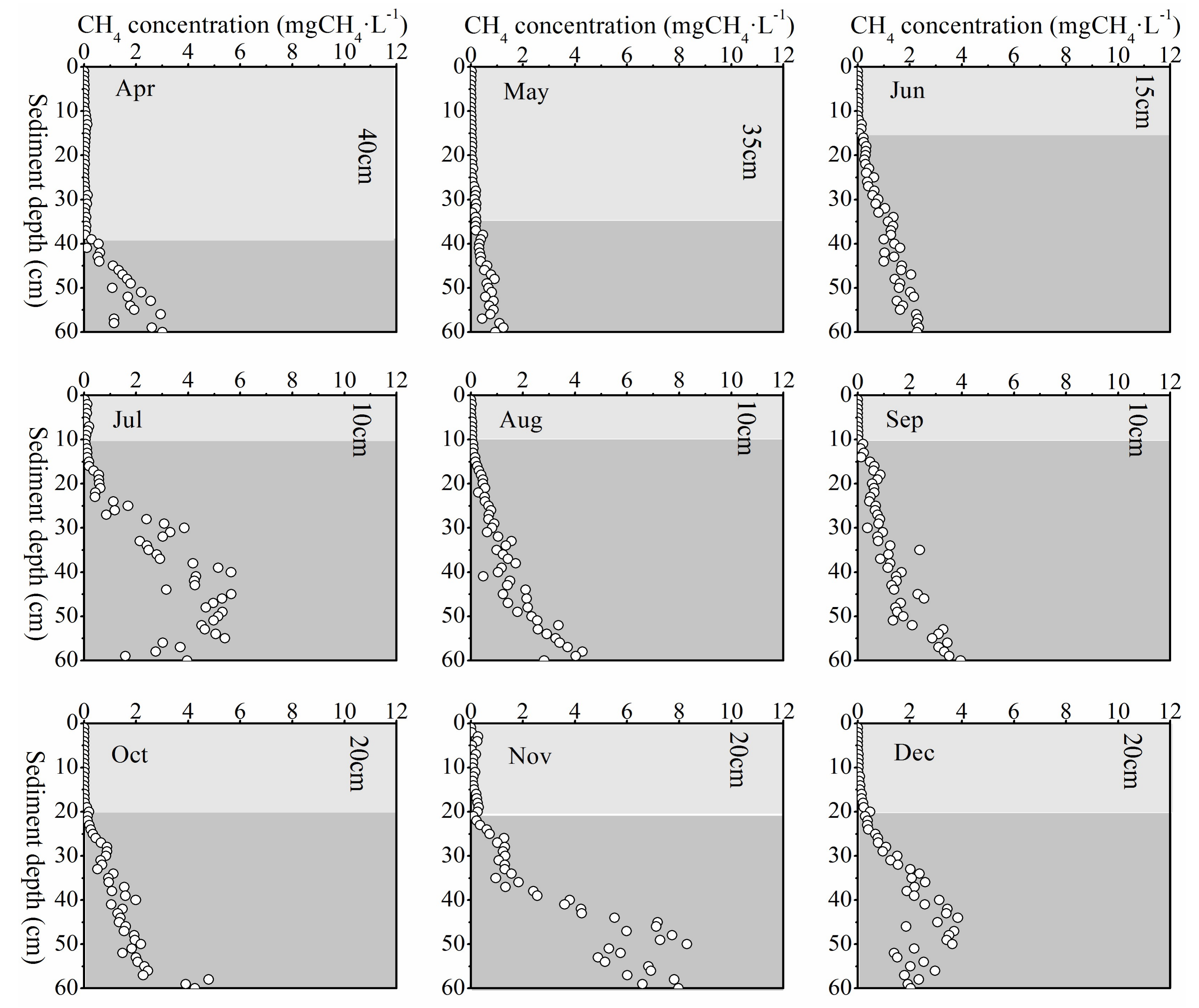
Top 1 cm pore-water CH4 concentration did not show any apparent seasonal variation. It was higher in the first half year and decreased to a lower value in the second half year (see Figure 3). Pore-water CH4 concentration in the top 1 cm was much lower than in the deeper layer sediment, resulting in a low diffusion flux. In the vertical profile, CH4 concentration increased significantly with depth. Although the pore-water CH4 concentration in deep sediment layers did not exhibit an apparent synchronously monthly variation with temperature, it did show an evident seasonal change (Figure 6). Pore-water CH4 concentration of deep sediment layer increased from May to July, decreased through October, and then reached the highest concentration (8.30 mgCH4·L−1) in November. After that, deep layer sediment pore-water CH4 concentration decreased again until the next April (Figure 6).
Along with the deep pore-water CH4 concentration variation, the depth of the steepest increase in CH4 concentration fluctuated up and down regularly during the year. The transition point of CH4 concentration increment usually occurred after the concentration exceeding 0.1 mgCH4·L−1. The location of this interface moved up from April to July and consistently stayed at about 10 cm depth through September, and then it went down from October to November (Figure 6).
Relationship between the pore-water CH4 concentration and total CH4 fluxes were also analyzed through Pearson correlation analysis. Significant correlations were observed between CH4 flux and pore-water CH4 concentration only at the depths of 11–15 cm (p < 0.05, R = 0.732) and 16–20 cm (p < 0.05, R = 0.777). (see Table 2).
4. Discussion
4.1. Dominant Mechanism of CH4 Emission
Different types of wetlands may be dominated by different CH4 emission patterns (plant mediated emission, bubble emission and the molecule diffusion) [39,40,41]. Anaerobic conditions in wetlands are favorable for CH4 production and accumulation, which finally create a CH4 concentration gradient between the underground and atmosphere [42]. Molecular diffusion is driven by the concentration gradient following Fick’s first law of diffusion [37]. Based on Fick’s first law, we calculated the molecular diffusive CH4 flux from the saltmarsh into the atmosphere. In this study, the calculated diffusion fluxes stayed at very low level with the highest diffusion flux of 0.55 mgCH4·m−2·day−1 in July. The proportion of diffusion fluxes accounted for 0.0048–5.53% of total monthly CH4 emission during the year. The specific reason for the weak diffusion flux is unclear due to the lack of ground water level, wind speed and the tide movement measurements. It is speculated that the wet condition in the saltmarsh is one of the most probable reasons, since it is known that water condition of the media can greatly influence the gas diffusion efficiency [43]. The S. mariqueter marsh in Yangtze estuary is located at the lower position of the tidal flat and was regularly submerged by the tide water. Surface sediments are always kept under a wet condition (this can be seen from the surface sediment water content in Table 1), which greatly inhibits the gas diffusion from surface sediment into air. In addition, the surface sediment usually stayed at a relative oxic condition, which can be seen from the low AVS concentrations in the surface sediment. Pore-water CH4 concentrations was significantly correlated with AVS concentrations (p < 0.01, R2 = 0.265). It was also proven in the previous study that oxygen could easily penetrate sediment creating an oxic condition when the sediment surface exposes to the air [44]. Previous studies reported that the existence of oxidizing zones can greatly reduce the diffusion CH4 flux. According to Yun et al. [45], the aerobic methanotrophs could oxidize more than 90% of the CH4 produced in the anoxic conditions. Similar results were also obtained by Liebner et al. [46] who found that the diffusive CH4 flux from the sediment surface only accounted for less than 2% of the total flux into the atmosphere in an alpine fen due to the linearly decreased pore water CH4 concentration at the depth of 0–15 cm. Our research also indicated that the intense oxidation of surface pore-water CH4 directly led to the weak diffusive CH4 flux.
In this study, S. mariqueter was found to facilitate CH4 emissions and the plant emitted more than 94% of the total CH4, which was consistent with many previous studies (Table 3). The highest chamber CH4 flux appeared in August when S. mariqueter was in the utmost abundant with the biggest aboveground biomass throughout the year of 692.6 g·m−2. The chamber CH4 fluxes of the three thriving months of S. mariqueter (July, August and September) constituted more than 80% of the total annual emission. The chamber CH4 flux decreased greatly at the end of growing season, which was consistent with the research of Chmura et al. [47]. The aerenchyma of wetland plants had two opposite effects on CH4 emission. Negatively, it could transport oxygen downward, creating an aerobic zone in rhizosphere [19]. The enhanced oxygen availability in sediment could inhibit CH4 production and accelerate CH4 consumption [46,48]. On the other hand, presence of aerenchyma in wetland plants also provides gas channels for CH4 escaping from underground to the atmosphere [16,49]. In a previous research of similar salt marsh, the net effect of these two processes was found to change along with the S. mariqueter growth stage [26]. It is indicated that the quantity of upward transported CH4 to the air through S. mariqueter exceeded the oxidized CH4 by downward transported O2 through S. mariqueter.
The fact that chamber CH4 fluxes were significantly correlated with aboveground biomass of S. mariqueter suggested significant effect of marsh plant growth on CH4 emission. Besides, regression analysis of different temperatures (air temperature and the sediment temperature at different depths 5 cm, 10 cm and 15 cm) and chamber CH4 fluxes revealed that CH4 fluxes were best fitted with the temperature at the sediment depth of 15 cm where the roots of S. mariqueter were concentrated [29] (Figure 5). This indicates that the rhizospheric temperature would be a good predictor of CH4 emission. While higher temperature usually leads to stronger methanogenesis and CH4 accumulation [50], our result emphasizes the significance of the temperature increase in rhizosphere that enhanced the CH4 emission. These observations further pointed to the great contribution of plant transportation to overall CH4 emissions in this salt marsh ecosystem. Previous research showed that the wetland plant, no matter living or dead, could provide a continuous escaping route for CH4 even in winter [51]. Nonetheless, our results indicated that the strongest transportation capacity of CH4 by individual plant appeared in August with the highest CH4 flux at 2.34 × 10⁻² mgCH4·stem−1·day−1 in these Yangtze estuary wetlands.
4.2. The Implication of Pore-Water CH4 Concentration for CH4 Emission
Static pore-water CH4 concentration from the surface to deep sediment was a net result of CH4 production and consumption, which could be affected by many environmental factors such as the redox potential, sediment organic carbon content, the distribution of methanogens and methanotroph, etc. [59,60,61]. In this study, the deep pore-water CH4 concentration did not exhibit synchronously seasonal variation with temperature (Figure 2), which was consistent with previous study in an alpine fen [46]. Sediment pore-water CH4 concentration profiles showed that there was an interface where the CH4 concentration steeply increased after it exceeded 0.1 mgCH4·L−1 (Figure 6). Although the CH4 concentration in the surface 10 cm sediment did not show apparent seasonal variations, the depth of this interface did vary and was shallower (~10 cm) in summer than in other seasons (Figure 6). Previous studies showed that the surface sediment pore-water CH4 concentration was influenced by the oxygen concentration easily and more than 90% of the CH4 produced in anoxic conditions could be oxidized in the upper aerobic conditions [62]. Conversely, the pore-water CH4 concentration could be seen as the indicator of environmental oxidation–deoxidation status. In our study, we attributed the upper layer of the sediment where CH4 concentration was lower than 0.1 mg CH4·L−1 to the active CH4 oxidization (aerobic and anaerobic). Above this interface, CH4 concentration was controlled by the aerobic and anaerobic oxidation process and maintained at a low level (Figure 5). Below this interface, CH4 concentration increased sharply, which was controlled by the anaerobic oxidation and production and diffusion from deeper layer. The effects of temperature on the depth of this “interface” could be explained from two aspects. On the one hand, under high temperature, oxygen penetration into sediment was generally reduced because the solubility of atmospheric oxygen decreased with temperature increase [44]. On the other hand, intensive respiration took place at high temperature, which accelerated the oxygen consumption within the surface sediment zones [63,64].
The analysis of the correlation between chamber CH4 fluxes and the pore-water CH4 concentration in different depths showed that only the pore-water CH4 concentration at the depths of 11–15 cm and 16–20 cm, where the dense roots of S. mariqueter are distributed, best predicted the chamber CH4 fluxes (see Table 2). The increased temperature in summer raised the depth of reactive layer for CH4 production to the depth of plant root distribution, which directly promoted the rhizospheric CH4 uptake from sediment pore water and prevented the CH4 oxidation in diffusion. The positively correlated chamber CH4 fluxes and rhizospheric CH4 concentration revealed that overall S. mariqueter acted as a promoter of CH4 emission when taking both rhizospheric CH4 oxidation and transportation into consideration.
The lack of significant relationship between the surface (0–10 cm) pore-water CH4 concentration and chamber CH4 fluxes further indicated the small contribution of gas molecular diffusion to CH4 emission. Although the pore-water CH4 concentration was apparently higher in the deeper layers, it had little effect on CH4 emission, probably because most of the upward diffusive CH4 was anaerobically oxidized due to the long-distance migration [64,65]. In addition, the CH4 in the deep sediment scantly contributed little to CH4 fluxes through bubble emission because the CH4 concentration was not high enough to form gas bubbles. Previous studies have indicated that bubbles could not form until pore-water CH4 concentrations exceeded 7.1–8.0 mgCH4·L−1 [66]. In this research, pore-water CH4 concentration in surface was only about 0.001–0.01 mgCH4·L−1, and even the highest pore-water CH4 concentration in deep sediment layer (below 45 cm) was under 8.0 mgCH4·L−1.
5. Conclusions
This study demonstrated that S. mariqueter marsh in Yangtze estuary acted as a net source of atmospheric CH4. The annual average chamber CH4 flux was 24.0 mgCH4·m−2·day−1 with the peak flux in August when the oxidization layer became shallow (about 10 cm) and the S. mariqueter thrived. The calculated diffusion CH4 fluxes were no more than 6% of the total fluxes, indicating that molecular diffusion was not a major pathway of CH4 emission in this salt marsh. Analysis of seasonal variation of pore-water CH4 concentration identified the dominant emission pattern as plant transport, which was evident by significantly positive correlation between CH4 concentrations in rhizosphere and chamber CH4 fluxes. In addition, generally low pore-water CH4 concentration (much less than 8.0 mg CH4 L−1) throughout the year prevented the formation of CH4 gas bubbles from ebullition. While wetland plant could exert an influence on rhizosphere CH4 oxidation, the transport function of the plant played a more important role in CH4 emission in the Yangtze estuary S. mariqueter marsh.
Acknowledgments
The authors are deeply indebted to Chu Wang and Huanguang Deng for their assistance with fieldwork and in the laboratory. This work was jointly supported by the National Natural Science Foundation of China (Grant No. 41473094 and No. 41671467), the Ministry of Science and Technology Project Foundation (2014FY210600), the Shanghai Municipal Natural Science Foundation (Grant No. ZR1412100), the research fund from the SKLEC (2015KYYW03), the Natural Science Project of Zhejiang Province (LQ18D060003 and LQ13D060003) and the Scientific Research Fund of the Second Institute of Oceanography, SOA (JG1515).
Author Contributions
Yangjie Li, Dongqi Wang and Zhenlou Chen designed the study; Yangjie Li, Dongqi Wang and Hong Hu performed the fieldwork and laboratory experiment; Yangjie Li wrote the manuscript; Dongqi Wang, Haiyan Jin and Jianfang Chen helped improve the manuscript before submission; and Dongqi Wang and Zhi Yang helped revise the manuscript according to the reviewers’ comments.
Conflicts of Interest
I would like to declare on behalf of my co-authors that the work was original research that has not been published previously, and is not under consideration for publication elsewhere, in whole or in part. All of the listed authors have approved the manuscript.
References
- IPCC. Climate Change 2013: The Physical Science Basis; Cambridge University Press: Cambridge, UK; New York, NY, USA, 2013. [Google Scholar]
- Keller, J.K.; Sutton-Grier, A.E.; Bullock, A.L.; Megonigal, J.P. Anaerobic metabolism in tidal freshwater wetlands: I. Plant removal effects on iron reduction and methanogenesis. Estuaries Coasts 2013, 36, 457–470. [Google Scholar] [CrossRef]
- Whiticar, M.J. Diagenetic relationships of methanogenesis, nutrients, acoustic turbidity, pockmarks and freshwater seepages in EckernfordeBay. Mar. Geol. 2002, 182, 29–53. [Google Scholar] [CrossRef]
- Moore, T.R.; Dalva, M. Methane and carbon dioxide exchange potentials of peat soils in aerobic and anaerobic laboratory incubations. Soil Biol. Biochem. 1997, 29, 1157–1164. [Google Scholar] [CrossRef]
- Segers, R. Methane production and methane consumption: A review of processes underlying wetland methane fluxes. Biogeochemistry 1998, 41, 23–51. [Google Scholar] [CrossRef]
- Tang, J.; Zhuang, Q.; Shannon, R.D.; White, J.R. Quantifying wetland methane emissions with process-based models of different complexities. Biogeosciences 2010, 7, 6121–6171. [Google Scholar] [CrossRef]
- Watson, A.; Stephen, K.D.; Nedwell, D.B.; Arah, J.R. Oxidation of methane in peat: Kinetics of CH4 and O2 removal and the role of plant roots. Soil Biol. Biochem. 1997, 29, 1257–1267. [Google Scholar] [CrossRef]
- Fritz, C.; Pancotto, V.A.; Elzenga, J.; Visser, E.J.; Grootjans, A.P.; Pol, A.; Iturraspe, R.; Roelofs, J.G.M.; Smolders, A.J. Zero methane emission bogs: Extreme rhizosphere oxygenation by cushion plants in Patagonia. New Phytol. 2011, 190, 398–408. [Google Scholar] [CrossRef] [PubMed] [Green Version]
- Smemo, K.A.; Yavitt, J.B. Anaerobic oxidation of methane: An underappreciated aspect of methane cycling in peatland ecosystems? Biogeosciences 2011, 8, 779–793. [Google Scholar] [CrossRef]
- Liu, D.Y.; Ding, W.X.; Jia, Z.J.; Cai, Z.C. Relation between methanogenic archaea and methane production potential in selected natural wetland ecosystems across China. Biogeosciences 2011, 8, 329–338. [Google Scholar] [CrossRef]
- Chowdhury, T.R.; Dick, R.P. Ecology of aerobic methanotrophs in controlling methane fluxes from wetlands. Appl. Soil Ecol. 2013, 65, 8–22. [Google Scholar] [CrossRef]
- Chanton, J.P. The effect of gas transport on the isotope signature of methane in wetlands. Org. Geochem. 2005, 36, 753–768. [Google Scholar] [CrossRef]
- Dingemans, B.J.; Bakker, E.S.; Bodelier, P.L. Aquatic herbivores facilitate the emission of methane from wetlands. Ecology 2011, 92, 1166–1173. [Google Scholar] [CrossRef] [PubMed]
- Kao-Kniffin, J.; Freyre, D.S.; Balser, T.C. Methane dynamics across wetland plant species. Aquat. Bot. 2010, 93, 107–113. [Google Scholar] [CrossRef]
- Lai, D.Y.F. Methane Dynamics in Northern Peatlands: A Review. Pedosphere 2009, 19, 409–421. [Google Scholar] [CrossRef]
- Belger, L.; Forsberg, B.R.; Melack, J.M. Carbon dioxide and methane emissions from interfluvial wetlands in the upper Negro River basin, Brazil. Biogeochemistry 2011, 105, 171–183. [Google Scholar] [CrossRef]
- Laanbroek, H.J. Methane emission from natural wetlands: Interplay between emergent macrophytes and soil microbial processes. A mini-review. Ann. Bot. 2010, 105, 141–153. [Google Scholar] [CrossRef] [PubMed]
- Larmola, T.; Tuittila, E.S.; Tiirola, M.; Nykänen, H.; Martikainen, P.J.; Yrjälä, K.; Tuomivirta, T.; Fritze, H. The role of Sphagnum mosses in the methane cycling of a boreal mire. Ecology 2010, 91, 2356–2365. [Google Scholar] [CrossRef] [PubMed]
- Cho, R.; Schroth, M.H.; Zeyer, J. Circadian methane oxidation in the root zone of rice plants. Biogeochemistry 2012, 111, 317–330. [Google Scholar] [CrossRef]
- Koelbener, A.; Ström, L.; Edwards, P.J.; Venterink, H.O. Plant species from mesotrophic wetlands cause relatively high methane emissions from peat soil. Plant Soil 2010, 326, 147–158. [Google Scholar] [CrossRef]
- Ding, W.; Cai, Z.; Tsuruta, H. Plant species effects on methane emissions from freshwater marshes. Atmos. Environ. 2005, 39, 3199–3207. [Google Scholar] [CrossRef]
- Bubier, J.L.; Moore, T.R.; Bellisario, L.; Comer, N.T.; Crill, P.M. Ecological controls on methane emissions from a northern peatland complex in the zone of discontinuous permafrost, Manitoba, Canada. Glob. Biogeochem. Cycles 1995, 9, 455–470. [Google Scholar] [CrossRef]
- Koh, H.S.; Ochs, C.A.; Yu, K. Hydrologic gradient and vegetation controls on CH4 and CO2 fluxes in a spring-fed forested wetland. Hydrobiologia 2009, 630, 271–286. [Google Scholar] [CrossRef]
- Juszczak, R.; Augustin, J. Exchange of the greenhouse gases methane and nitrous oxide between the atmosphere and a temperate peatland in central Europe. Wetlands 2013, 33, 895–907. [Google Scholar] [CrossRef]
- Chen, X.; Zong, Y. Coastal erosion along the Changjiang deltaic shoreline, China: History and prospective. Estuar. Coast. Shelf Sci. 1998, 46, 733–742. [Google Scholar] [CrossRef]
- Wang, D.; Chen, Z.; Xu, S. Methane emission from Yangtze estuarine wetland, China. J. Geophys. Res. 2009, 114, G02011. [Google Scholar] [CrossRef]
- Bu, N.S.; Qu, J.F.; Zhao, H.; Yan, Q.W.; Zhao, B.; Fan, J.L.; Fang, C.M.; Li, G. Effects of semi-lunar tidal cycling on soil CO2 and CH4 emissions: A case study in the Yangtze River estuary, China. Wetl. Ecol. Manag. 2015, 23, 727–736. [Google Scholar] [CrossRef]
- Yin, S.; An, S.; Deng, Q.; Zhang, J.; Ji, H.; Cheng, X. Spartina alterniflora invasions impact CH4 and N2O fluxes from a salt marsh in eastern China. Ecol. Eng. 2015, 81, 192–199. [Google Scholar] [CrossRef]
- Sun, S.; Cai, Y.; An, S. Differences in morphology and biomass allocation of Scirpus mariqueter between creekside and inland communities in the Changjiang estuary, China. Wetlands 2002, 22, 786–793. [Google Scholar] [CrossRef]
- Sun, S.; Gao, X.; Cai, Y. Variations in sexual and asexual reproduction of Scirpus mariqueter along an elevational gradient. Ecol. Res. 2001, 16, 263–274. [Google Scholar] [CrossRef]
- Yu, Z.; Li, Y.; Deng, H.; Wang, D.; Chen, Z.; Xu, S. Effect of Scirpus mariqueter on nitrous oxide emissions from a subtropical monsoon estuarine wetland. J. Geophys. Res. 2012, 117. [Google Scholar] [CrossRef]
- Khalil, M.A.K.; Rasmussen, R.A.; Wang, M.X.; Ren, L. Emissions of trace gases from Chinese rice fields and biogas generators: CH4, N2O, CO, CO2, chlorocarbons, and hydrocarbons. Chemosphere 1990, 20, 207–226. [Google Scholar] [CrossRef]
- Nelson, D.W.; Sommers, L.E.; Sparks, D.L.; Page, A.L.; Helmke, P.A.; Loeppert, R.H.; Soltanpour, P.N.; Tabatabai, M.A.; Sumner, M.E. Total carbon, organic carbon, and organic matter. In Methods of Soil Analysis. Part 3—Chemical Methods; Soil Science Society of America, American Society of Agronomy: Madison, WI, USA, 1996; pp. 961–1010. [Google Scholar]
- Grasshof, K.; Ehrhard, M.; Kremling, K. Methods of Seawater Analysis, 2nd ed.; Verlag Chemie: Weiheim, Germany, 1983. [Google Scholar]
- Lin, Y.H.; Guo, M.X.; Zhuang, Y. Determination of acid volatilesulfide and simultaneously extracted metals in sediment. Acta Sci. Circumstantiae 1997, 17, 353–358. (In Chinese) [Google Scholar]
- Lee, B.G.; Griscom, S.B.; Lee, J.S.; Choi, H.J.; Koh, C.H.; Luoma, S.N.; Fisher, N.S. Influences of dietary uptake and reactive sulfides onmetal bioavailability from aquatic sediments. Science 2000, 287, 282–284. [Google Scholar] [CrossRef] [PubMed]
- Hornibrook, E.R.C.; Bowes, H.L.; Culbert, A.; Gallego-Sala, A.V. Methanotrophy potential versus methane supply by pore water diffusion in peatlands. Biogeosciences 2009, 6, 1491–1504. [Google Scholar] [CrossRef] [Green Version]
- Lerman, A. Geochemical Processes: Water and Sediment Environments; John Wiley: New York, NY, USA, 1979; 481p. [Google Scholar]
- Rose, C.; Crumpton, W.G. Spatial patterns in dissolved oxygen and methane concentrations in a prairie pothole wetland in Iowa, USA. Wetlands 2006, 26, 1020–1025. [Google Scholar] [CrossRef]
- Shoemaker, J.K.; Varner, R.K.; Schrag, D.P. Characterization of subsurface methane production and release over 3 years at a New Hampshire wetland. Geochim. Cosmochim. Acta 2012, 91, 120–139. [Google Scholar] [CrossRef]
- Wang, Y.; Yang, H.; Ye, C.; Chen, X.; Xie, B.; Huan, C.; Zhang, J.; Xu, M. Effects of plant species on soil microbial processes and CH4 emission from constructed wetlands. Environ. Pollut. 2013, 174, 273–278. [Google Scholar] [CrossRef] [PubMed]
- Miao, Y.; Song, C.; Wang, X.; Sun, X.; Meng, H.; Sun, L. Greenhouse gas emissions from different wetlands during the snow-covered season in Northeast China. Atmos. Environ. 2012, 62, 328–335. [Google Scholar] [CrossRef]
- Aubertin, M.; Aachib, M.; Authier, K. Evaluation of diffusive gas flux through covers with a GCL. Geotext. Geomembr. 2000, 18, 215–233. [Google Scholar] [CrossRef]
- Rasmussen, H.; Jørgensen, B.B. Microelectrode studies of seasonal oxygen uptake in a coastal sediment: Role of molecular diffusion. Mar. Ecol. Prog. Ser. 1992, 81, 289–303. [Google Scholar] [CrossRef]
- Yun, J.; Yu, Z.; Li, K.; Zhang, H. Diversity, abundance and vertical distribution of methane-oxidizing bacteria (methanotrophs) in the sediments of the Xianghai wetland, Songnen Plain, northeast China. J. Soils Sediments 2013, 13, 242–252. [Google Scholar] [CrossRef]
- Liebner, S.; Schwarzenbach, S.P.; Zeyer, J. Methane emissions from an alpine fen in central Switzerland. Biogeochemistry 2012, 109, 287–299. [Google Scholar] [CrossRef]
- Chmura, G.L.; Kellman, L.; Guntenspergen, G.R. The greenhouse gas flux and potential global warming feedbacks of a northern macrotidal and microtidal salt marsh. Environ. Res. Lett. 2011, 6, 044016. [Google Scholar] [CrossRef]
- Askaer, L.; Elberling, B.; Glud, R.N.; Kühl, M.; Lauritsen, F.R.; Joensen, H.P. Soil heterogeneity effects on O2 distribution and CH4 emissions from wetlands: In situ and mesocosm studies with planar O2 optodes and membrane inlet mass spectrometry. Soil Biol. Biochem. 2010, 42, 2254–2265. [Google Scholar] [CrossRef]
- Song, H.; Liu, X. Anthropogenic effects on fluxes of ecosystem respiration and methane in the Yellow River Estuary, China. Wetlands 2016, 36, 113–123. [Google Scholar] [CrossRef]
- Jerman, V.; Metje, M.; Mandić-Mulec, I.; Frenzel, P. Wetland restoration and methanogenesis: The activity of microbial populations and competition for substrates at different temperatures. Biogeosciences 2009, 6, 1127–1138. [Google Scholar] [CrossRef]
- Brix, H. Gas exchange through dead culms of reed, Phragmites australis (Cav.) Trin. ex Steudel. Aquat. Bot. 1989, 35, 81–98. [Google Scholar] [CrossRef]
- Holzapfel-Pschorn, A.; Conrad, R.; Seiler, W. Effects of vegetation on the emission of methane from submerged paddy soil. Plant Soil 1986, 92, 223–233. [Google Scholar] [CrossRef]
- Schütz, H.; Holzapfel-Pschorn, A.; Conrad, R.; Rennenberg, H.; Seiler, W. A 3-year continuous record on the influence of daytime, season, and fertilizer treatment on methane emission rates from an Italian rice paddy. J. Geophys. Res. Atmos. 1989, 94, 16405–16416. [Google Scholar] [CrossRef]
- Butterbach-Bahl, K.; Papen, H.; Rennenberg, H. Impact of gas transport through rice cultivars on methane emission from rice paddy fields. Plant Cell Environ. 1997, 20, 1175–1183. [Google Scholar] [CrossRef]
- King, J.Y.; Reeburgh, W.S.; Regli, S.K. Methane emission and transport by arctic sedges in Alaska: Results of a vegetation removal experiment. J. Geophys. Res. Atmos. 1998, 103, 29083–29092. [Google Scholar] [CrossRef]
- Kelker, D.; Chanton, J. The effect of clipping on methane emissions from Carex. Biogeochemistry 1997, 39, 37–44. [Google Scholar] [CrossRef]
- Green, S.M.; Baird, A.J. A mesocosm study of the role of the sedge Eriophorum angustifolium in the efflux of methane—including that due to episodic ebullition-from peatlands. Plant Soil 2012, 351, 207–218. [Google Scholar] [CrossRef]
- Waddington, J.M.; Roulet, N.T.; Swanson, R.V. Water table control of CH4 emission enhancement by vascular plants in boreal peatlands. J. Geophys. Res. Atmos. 1996, 101, 22775–22785. [Google Scholar] [CrossRef]
- Stanley, E.H.; Ward, A.K. Effects of vascular plants on seasonal pore water carbon dynamics in a lotic wetland. Wetlands 2010, 30, 889–900. [Google Scholar] [CrossRef]
- Martens, C.S.; Albert, D.B.; Alperin, M.J. Biogeochemical processes controlling methane in gassy coastal sediments—Part 1. A model coupling organic matter flux to gas production, oxidation and transport. Cont. Shelf Res. 1998, 18, 1741–1770. [Google Scholar] [CrossRef]
- Borrel, G.; Jézéquel, D.; Biderre-Petit, C.; Morel-Desrosiers, N.; Morel, J.P.; Peyret, P.; Fonty, G.; Lehours, A.C. Production and consumption of methane in freshwater lake ecosystems. Res. Microbiol. 2011, 162, 832–847. [Google Scholar] [CrossRef] [PubMed]
- Frenzel, P.; Thebrath, B.; Conrad, R. Oxidation of methane in the oxic surface layer of a deep lake sediment (Lake Constance). FEMS Microbiol. Lett. 1990, 73, 149–158. [Google Scholar] [CrossRef]
- Nielsen, L.P.; Christensen, P.B.; Revsbech, N.P.; Sørensen, J. Denitrification and oxygen respiration in biofilms studied with a microsensor for nitrous oxide and oxygen. Microb. Ecol. 1990, 19, 63–72. [Google Scholar] [CrossRef] [PubMed]
- Valentine, D.L.; Reeburgh, W.S. New perspectives on anaerobic methane oxidation. Environ. Microbiol. 2000, 2, 477–484. [Google Scholar] [CrossRef] [PubMed]
- Caldwell, S.L.; Laidler, J.R.; Brewer, E.A.; Eberly, J.O.; Sandborgh, S.C.; Colwell, F.S. Anaerobic oxidation of methane: Mechanisms, bioenergetics, and the ecology of associated microorganisms. Environ. Sci. Technol. 2008, 42, 6791–6799. [Google Scholar] [CrossRef] [PubMed]
- Baird, A.J.; Beckwith, C.W.; Waldron, S.; Waddington, J.M. Ebullition of methane-containing gas bubbles from near-surface Sphagnum peat. Geophys. Res. Lett. 2004, 31. [Google Scholar] [CrossRef]
Figure 1.
The sampling site in Yangtze estuary. The studied salt marsh was mainly dominated by the endemic species of S. mariqueter.
Figure 1.
The sampling site in Yangtze estuary. The studied salt marsh was mainly dominated by the endemic species of S. mariqueter.
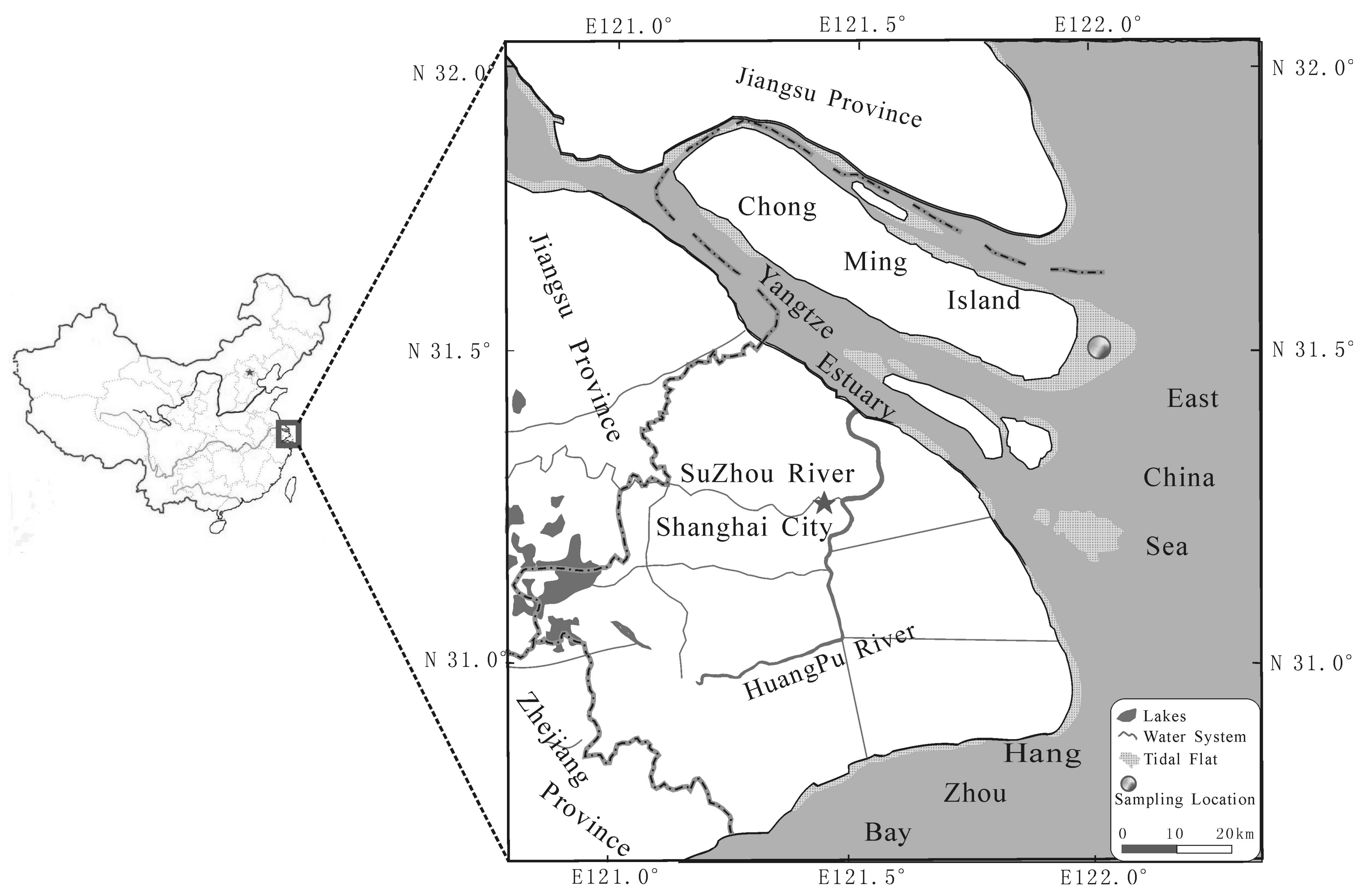
Figure 2.
AVS distribution in the sediment profile.
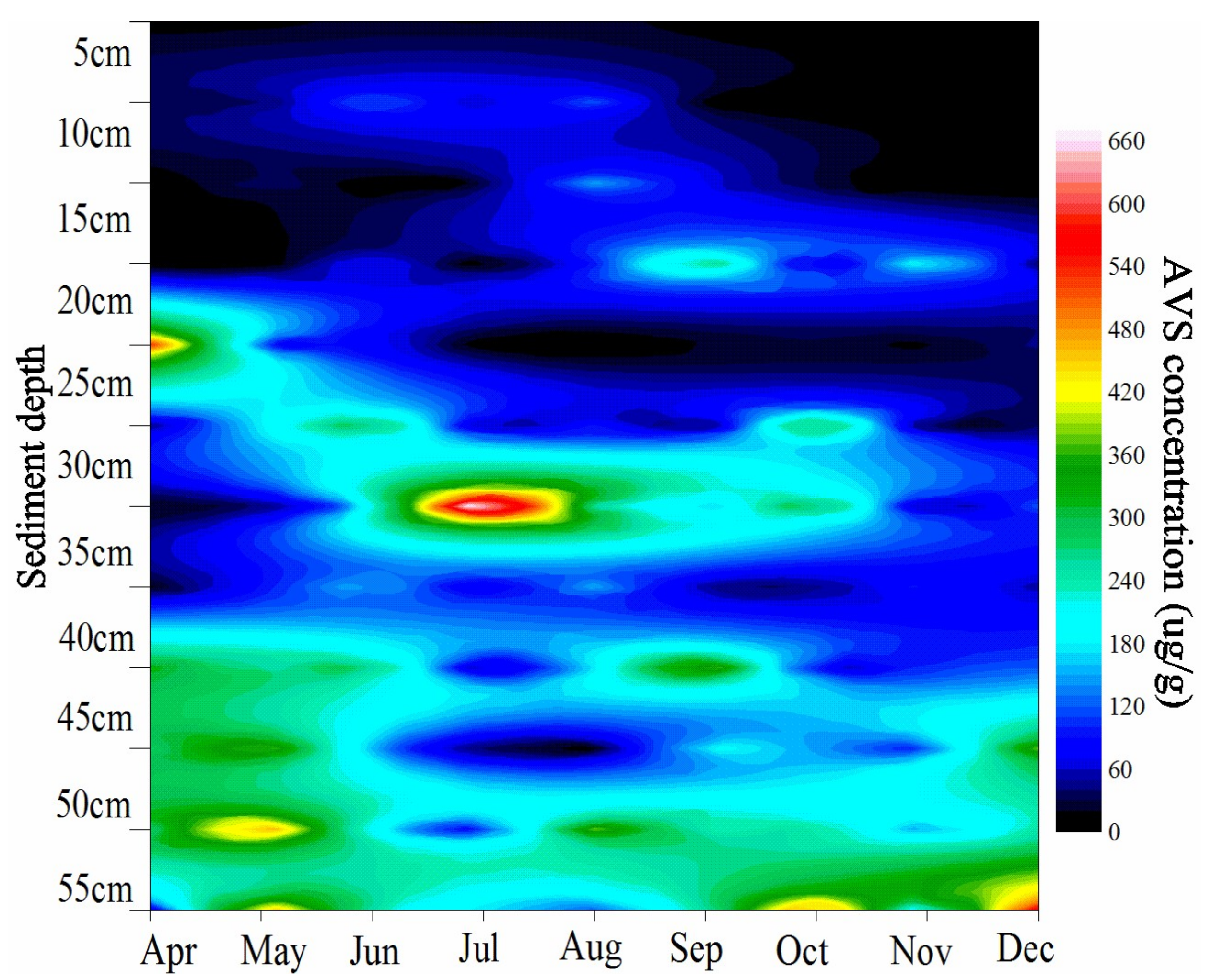
Figure 3.
The total chamber CH4 fluxes, calculated diffusion CH4 fluxes, the top 1 cm pore-water CH4 concentration and the biomass of S. mariqueter in each month during the year. CH4 fluxes are presented as column graphs, while the pore-water CH4 concentration and biomass are presented as line and symbol graphs. The black graphs in the figure are integrated with the left black Y axis and the blue graphs are integrated with the right blue Y axis.

Figure 4.
Correlation relationship between the CH4 fluxes and the aboveground biomass of S. mariqueter.
Figure 4.
Correlation relationship between the CH4 fluxes and the aboveground biomass of S. mariqueter.

Figure 5.
Relationship between chamber CH4 fluxes and temperature. Abbreviations: 5 cm GT, 10 cm GT and 15 cm GT represent the sediment temperature at depths of 5 cm, 10 cm and 15 cm, respectively (n = 70).
Figure 5.
Relationship between chamber CH4 fluxes and temperature. Abbreviations: 5 cm GT, 10 cm GT and 15 cm GT represent the sediment temperature at depths of 5 cm, 10 cm and 15 cm, respectively (n = 70).
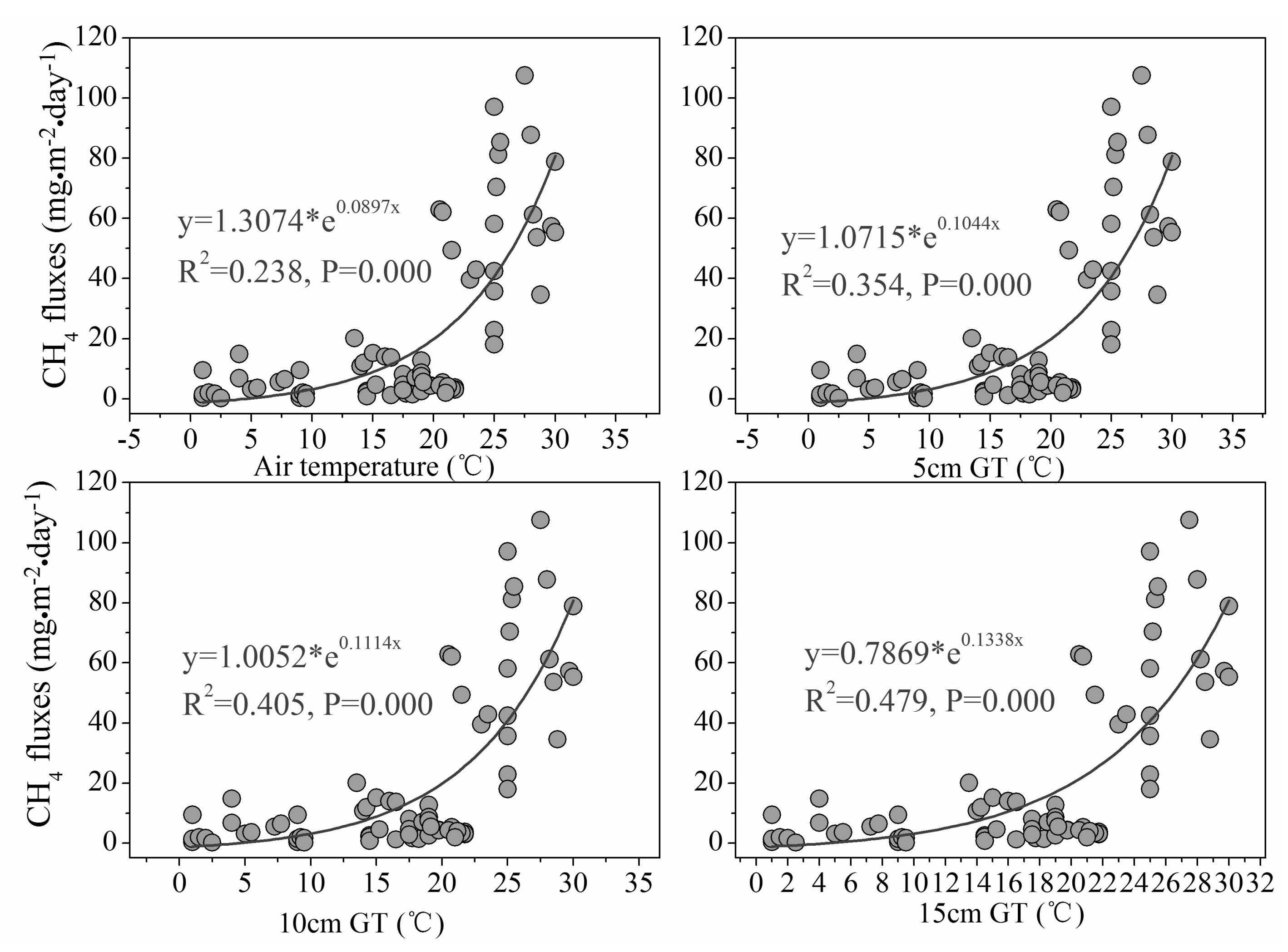
Figure 6.
Monthly variation of pore-water CH4 concentration. A steep increase in pore-water CH4 concentration occurred when it exceeded 0.1 mgCH4·L−1 for each month. The light color located above the depth of this steep increase indicates the low CH4 concentrations, while the dark color indicates the high CH4 concentrations.

Table 1.
Climatic, plant and soil physiochemical parameters of experimental site.
| Month | Temperature (°C) | PAR (W·m−2) | Biomass | SOC (g·dm·kg) | SWC (%) | APS/MD (μm) | NH4+-N (mg·kg−1) | NO3−-N (mg·kg−1) | AVS (μg·g−1) | |||||
|---|---|---|---|---|---|---|---|---|---|---|---|---|---|---|
| AAT | ATR | GT5 | GT10 | GT15 | (g·dm·m−2) | Number of Living Shoots in 50 cm × 50 cm Quadrats | ||||||||
| February | 4 | −2.0~9.0 | 3 | 2 | 1 | 8~266 | - | - | 7.27 | 43 | 16.81/23.81 | 3.04 | 0.15 | - |
| March | 12 | 7.5~14.5 | 10 | 9 | 9 | 17~233 | - | - | 6.91 | 39 | 15.06/20.23 | 4.88 | 0.19 | 7.46 |
| April | 25 | 16.0~28.0 | 20 | 20 | 17 | 15~304 | 44.6 | 66 | 7.59 | 36 | 14.31/20.07 | 7.54 | 0.12 | 1.37 |
| May | 23 | 15.5~29.5 | 23 | 21 | 20 | 35~317 | 105.9 | 223 | 6.78 | 55 | 12.51/16.86 | 4.82 | 0.98 | 14.3 |
| June | 27 | 25.0~28.5 | 26 | 26 | 26 | 30~145 | 433.9 | 403 | 7.86 | 54 | 7.747/9.527 | 5.65 | 0.49 | 6.35 |
| July | 33 | 30.0-35.5 | 31 | 32 | 29 | 38~297 | 364.1 | 445 | 8.42 | 66 | 7.129/8.744 | 4.33 | ND | 8.28 |
| August | 25 | 23.5~26.0 | 25 | 25 | 25 | 15~98 | 692.6 | 972 | 7.12 | 91 | 6.636/7.891 | 4.98 | 0.59 | 3.43 |
| September | 20 | 16.0~25.0 | 25 | 24 | 23 | 38~313 | 534.1 | 869 | 7.65 | 46 | 7.402/9.479 | 4.48 | 0.49 | 11.5 |
| October | 22 | 16.0~24.0 | 21 | 21 | 20 | 24~284 | 263.9 | 623 | 8.01 | 55 | 8.317/10.81 | 4.06 | 0.10 | 7.32 |
| November | 11 | 5.5.0~14.0 | 14 | 14 | 14 | 19~222 | - | - | 7.78 | 69 | 8.082/10.28 | 5.25 | 0.16 | 12.5 |
| December | 7 | −1.0~9.5.0 | 7 | 6 | 6 | 8~188 | 130.3 | - | 7.63 | 65 | 9.096/11.92 | 4.07 | 0.20 | - |
AAT: average air temperature; ATR: Air temperature range during the sampling day; GT5: Sediment temperature at the depth of 5 cm; GT10: Sediment temperature at the depth of 10 cm; GT15: Sediment temperature at the depth of 15 cm) are the mean value of the daily variation. PAR (Photosynthetically Active Radiation) is shown as the variation range of the daily continuous observations. SOC is the average soil organic carbon values of the surface 25 cm sediments. The rest of the sediment parameters (SWC, APS, MD, NH4+-N, NO3−-N and AVS) are the values of the surface 1 cm sediment.
Table 2.
Correlation relationships between monthly methane (CH4) fluxes and the pore-water CH4 concentration at the different depths a, * p < 0.05.
Table 2.
Correlation relationships between monthly methane (CH4) fluxes and the pore-water CH4 concentration at the different depths a, * p < 0.05.
| Depth | CH4 Fluxes b | Depth | CH4 Fluxes | Depth | CH4 Fluxes |
|---|---|---|---|---|---|
| 0–5 cm | −0.084 | 21–25 cm | 0.590 | 41–45 cm | −0.034 |
| 6–10 cm | 0.146 | 26–30 cm | 0.192 | 46–50 cm | −0.065 |
| 11–15 cm | 0.732 * | 31–35 cm | 0.279 | 51–55 cm | 0.219 |
| 16–20 cm | 0.777 * | 36–40 cm | 0.101 | 56–60 cm | 0.190 |
a The pore-water CH4 concentration was measured at 1-cm interval, but the mean of the pore-water CH4 concentrations at 5-cm interval was used to analyze the correlation relationship between the CH4 fluxes and the underground CH4 concentrations at different depths of each month. b The correlation coefficient “R” for CH4 fluxes and the averaged pore-water CH4 concentrations in different depths.
Table 3.
Plant contributions of different species to CH4 emissions.
| Vegetation Type | Proportion of Plant Emitted CH4 (%) a | Plant Treatment b | References |
|---|---|---|---|
| C. lasiocarpa | 73~82 | clipping c | [21] |
| C. meyeriana | 75~86 | clipping | [21] |
| Rice | 94 | clipping | [52] |
| Rice | 97 | clipping | [53] |
| Rice | 90 | clipping | [54] |
| Reed | 60 | clipping | [52] |
| Weeds | 84 | clipping | [52] |
| Sedge | 79 | uprooting d | [55] |
| Eriophorum latifolium | 80 | uprooting | [20] |
| Sedge | 94 | clipping | [56] |
| Sedge | 83 | clipping | [57] |
| E. vaginatum | 88 | clipping | [58] |
a The proportion of plant transported CH4 fluxes in the total CH4 fluxes. b Different approaches to quantify the plants’ effects on CH4 emissions. c,d The most commonly adopted approaches in studying the plant transportation capacity for CH4. c The plant stems covered by the static closed chamber were clipped leaving the stem section on the sediment surface; d Plants covered by the static closed chamber were uprooted.
© 2018 by the authors. Licensee MDPI, Basel, Switzerland. This article is an open access article distributed under the terms and conditions of the Creative Commons Attribution (CC BY) license (http://creativecommons.org/licenses/by/4.0/).
Share and Cite
MDPI and ACS Style
Li, Y.; Wang, D.; Chen, Z.; Jin, H.; Hu, H.; Chen, J.; Yang, Z. Role of Scirpus mariqueter on Methane Emission from an Intertidal Saltmarsh of Yangtze Estuary. Sustainability 2018, 10, 1139. https://doi.org/10.3390/su10041139
AMA Style
Li Y, Wang D, Chen Z, Jin H, Hu H, Chen J, Yang Z. Role of Scirpus mariqueter on Methane Emission from an Intertidal Saltmarsh of Yangtze Estuary. Sustainability. 2018; 10(4):1139. https://doi.org/10.3390/su10041139
Chicago/Turabian StyleLi, Yangjie, Dongqi Wang, Zhenlou Chen, Haiyan Jin, Hong Hu, Jianfang Chen, and Zhi Yang. 2018. "Role of Scirpus mariqueter on Methane Emission from an Intertidal Saltmarsh of Yangtze Estuary" Sustainability 10, no. 4: 1139. https://doi.org/10.3390/su10041139
Note that from the first issue of 2016, this journal uses article numbers instead of page numbers. See further details here.