Research on the Topological Properties of Air Quality Index Based on a Complex Network

Abstract

To analyze the dynamic characteristics of air quality for enforcing effective measures to prevent and evade air pollution harm, air quality index (AQI) time series data was selected and transformed into a symbol sequence consisting of characters (H, M, L) through the coarse graining process; then each 6-symbols series was treated as one vertex by time sequence to construct the AQI directed-weighted network; finally the centrality, clusterability, and ranking of the AQI network were analyzed. The results indicated that vertex strength and cumulative strength distribution, vertex strength and strength rank presented power law distributions, and the AQI network is a scale-free network. Only 17 vertices possessed a higher weighted clustering coefficient; meanwhile weighted clustering coefficient and vertex strength didn’t show a strong correlation. The AQI network did not have an obvious central tendency towards intermediaries in general, but 20.55% of vertices accounted for nearly 1/2 of the intermediaries, and the varieties still existed. The mean distance of 68.4932% of vertices was 6.120–9.973, the AQI network did not have obvious small-world phenomena, the conversion of AQI patterns presented the characteristics of periodicity and regularity, and 20.2055% of vertices had high proximity prestige. The vertices fell into six islands, the AQI pattern indicating heavy or serious air pollution lasting six days always lingered for a long time. The number of triads 2-012 was the largest, and the AQI network followed the transitivity model. The study has instructional significance in understanding time change regulation of air quality in Beijing, opening a new way for time series prediction research. Additionally, the factors causing the change of topological properties should be analyzed in the future research.

1. Introduction

Air pollution is hazardous chemicals released into the atmosphere by a number of natural and/or anthropogenic activities. The change of atmospheric composition is attributed to the combustion of fossil fuels [1]. Air pollutants, such as carbon monoxide (CO), respirable particulate matter (PM_2.5 and PM₁₀), nitrogen oxides (NO_x), ozone (O₃), sulphur dioxide (SO₂), nitrogen dioxide (NO₂), and nitric oxide (NO), differ in their reaction properties, chemical composition, time of disintegration, emission, and diffuse ability over short or long distances. Air pollution has both acute and chronic impacts on human health, and causes or aggravates numerous organic and systemic diseases, such as heart disease, respiratory irritation, lung cancer, chronic bronchitis, and acute respiratory infections, which will bring about premature mortality and reduce life expectancy [2,3,4]. Therefore, air pollution is a fundamental issue of global concern. Atmospheric pollution in China is very serious. The “Environmental Performance Index: 2016 Report” released by Yale University showed that as the world’s second largest economy, the air quality in China was the second-lowest in the world, only slightly better than in Bangladesh, and even India was still ahead of China [5]. China has become a disaster area of air pollution in the world, and air pollution has largely covered the vast majority of the country. Especially in recent years, foggy and hazy weather has frequently attacked Northern and Eastern China, making air pollution control the most prominent and urgent environmental problem at present.

The AQI is a simple and generalized scale or indicator to assess air quality status. The AQI in China is developed based on GB3095-2012, introduced by the ministry of environmental protection of the People’s Republic of China, which covers six pollutants, including PM₁₀, PM_2.5, SO₂, CO, NO₂, and O₃ [6]. According to air quality standards (GB3095-2012), the AQI could be divided into six levels: excellent (0~50), good (51~100), mild pollution (101~150), moderate pollution (151~200), heavy pollution (201~300), and serious pollution (>300). As the AQI increases, the pollution level increases. For the government, the AQI is a powerful tool for formulating policies related to air quality management and pollution mitigation measures; meanwhile it is also an important index for the general public to rapidly estimate the air quality condition. Thus, the reliable and effective forecasting of the AQI is significantly important, because it can be used to enforce appropriate suggestions and regulations for preventing and evading air pollution damage.

The empirical methods to forecast various air quality indexes generally fall into four categories: the autoregressive integrated moving average method (ARIMA), multiple linear method (MLR), artificial neural networks (ANNs), and hybrid methods [7]. The ARIMA is a traditional forecasting technique, widely used for analyzing nonlinear time series data [8,9]. However, it is constrained by the assumptions of stationarity and linearity, and only suitable for the linear form of time series data [10]. The MLR method is a classical statistical techniques compared to other approaches. Due to its accuracy of interpretation, the MLR also remains useful and widely used in the prediction field [11,12]. However, the MLR can’t capture the non-linear relationships between input and output variables and is not suitable for complex systems [13].

The ANNs is characterized by self-learning, self-organization, strong mapping ability, and generalization, which can implement approximating nonlinear functions with arbitrary accuracy; thus, the ANNs can perform better than traditional statistical models for forecasting AQI [14,15,16,17,18]. However, an ANN is unable to present a clear formula for the forecasting model [19,20,21]. Almost as remarkably, many studies successfully and widely employed the hybrid model in pollution index forecasting and proved that the hybrid model generally had more precise forecasts than the monomial forecast model [7,8,10,22,23,24].

The analysis of the AQI time series is difficult because of the irregularity, randomness, and non-stationarity. The existing research methods, such as ARIMA, MLR, ANNs, and hybrid model, are just a forecast of time series data, and cannot capture the pattern information and change law hidden behind AQI fluctuation. This make it difficult to answer the following questions: What patterns exist in the AQI change? Which patterns are the most vital and play a leading role? Is there a huge gap in the influence of AQI patterns? Which patterns are closer to others and easily change? Which patterns are the hub of AQI pattern transformation and essential to control the air pollution diffusion? Are there disparate subgroups or clusters in the AQI network? What are the characteristics of each subgroup or cluster? Is there a hierarchy or ranking in the AQI network? Which vertices have higher ranking? Are there small-world phenomena or scale-free properties in the AQI network? Obviously, the answers to these questions are crucial for revealing the AQI fluctuation law and internal mechanisms, and can also provide evidence for formulating the measures about preventing and controlling air pollution. Our study will construct an AQI directed-weighted network by transforming time series data into a symbol sequence, apply complex network theory to analyze the topological properties, and give answers to the above questions. Meanwhile, our study also provides a methodological perspective and ideas for time series forecast, contributing to existing studies.

On the other hand, although complex network theory has been used across many science fields in recent years, only a few studies have conducted complex network theory on the time series forecasting. For instance, Gao, An, Liu, and Ding (2011) used a complex network to analyze the linkage between crude oil future prices and spot price from 25 November 2002 to 24 September 2010 [25]. Wan, Shu, and Guo (2012) presented a method to model frequent patterns and their interaction relationship in sequences based on a complex network [26]. Zhou, Gong, Zhi, and Feng (2008) collected data of the surface temperature from 160 Chinese weather observations and investigated the topology of Chinese climate networks by using a complex network [27]. Until now, few scholars have established an AQI network and used complex network theory to study the AQI change law. Therefore, this study is undertaken to analyze the AQI time series data with complex network theory, to fill the research gap.

This study selected the time serial data of the AQI in Beijing from 1 November 2013 to 31 October 2017; transformed it into a symbol sequence consisting of three characters {H, M, L} through the coarse graining process; then defined 272 AQI patterns as vertices to create one directed-weighted network of the AQI via sliding sequence; and finally analyzed the topological properties of vertex strength, strength distribution, weighted clustering coefficient, betweenness centralization, islands, distance, proximity prestige, ranking and triadic.

The rest of this article is organized as follows. The data and complex network theory are introduced, and the AQI complex network is constructed in Section 2. The topological properties of the AQI complex network are analyzed in Section 3. At last, conclusions are summarized and future research is suggested in Section 4.

2. Data and Method

2.1. Data Description

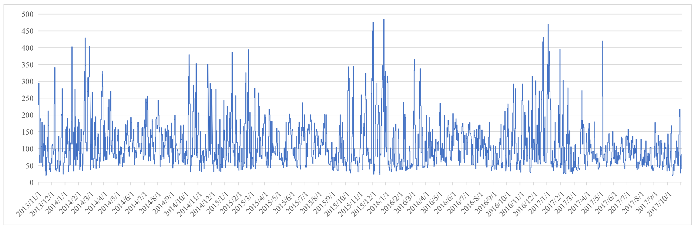
The data used in the study is the AQI of Beijing from 1 November 2013 to 31 October 2017 (Figure 1), which was obtained from the China National Environmental Monitoring Centre (http://www.cnemc.cn/).

2.2. Complex Network Theory

The complex network is a system composed of a mass of vertices and edges, which considers distinct elements or actors represented by vertices (or nodes) and the interaction or relationship between the elements or actors as edges (or links), usually shown as a graph to describe phenomena in social or natural sciences. Nowadays, the complex network is widely used in various scientific fields, such as biological networks, telecommunication networks, social networks, cognitive and semantic networks, and computer networks. It draws on theories and methods including graph theory from mathematics, information visualization from computer science, statistical mechanics from physics, social structure from sociology, and inferential modeling from statistics [28].

Complex networks are very different from traditional statistical methods. For example, in social sciences, traditional statistical methods carry out research based on attribute data, such as gender, age, income, attitudes, shared values, etc. However, individuals live in a particular social environment, and their behavior is affected by others. Statistical methods, like a “meat grinder”, divorce individuals from the social context in which they live and assume that there are no relations between individuals. In contrast, the complex network conducts research on the basis of relational data, and captures attitudes and behaviors determined by social structures through relationship analysis [29].

The characteristic analysis of complex network mainly includes centrality analysis, clusterability analysis, ranking analysis, and network type analysis. The central analysis is to find influential vertices, the clusterability analysis is for discovering cohesive subgroups from the network, and the ranking analysis is for extracting discrete ranks from relations. The scale-free network and small-world network are the most common network types (

Table 1. Complex network characteristic analysis.

Type	Content	Measurement	Description
Network Property	Network Centrality Analysis	Degree Centrality (Vertex Strength)	Assessing the influences of network vertices
		Closeness Centrality (Weighted Clustering Coefficient)
		Between Centrality
Network Structure	Network Clusterability Analysis	Island Analysis	Discovering cohesive subgroups from network
	Network Ranking Analysis	Prestige Analysis	Extracting the discrete ranks of network vertices
		Triadic Analysis
Network Type	Scale-Free Network	Power-Law Distribution	Exposing network types
	Small-World Network	Characteristic Path Length
		Clustering Coefficient

).

The measurement indicators of centrality analysis include degree centrality, closeness centrality, and between centrality. Degree centrality is a simple measure that counts how many neighbors a vertex has. The more neighbors, the more important the vertex. Closeness centrality measures the mean distance from a vertex to other vertices. Betweenness centrality measures the extent to which a vertex lies on paths between other vertices. In a weighted network, the degree centrality and closeness centrality are usually measured by vertex strength and weighted clustering coefficient.

Network clusterability analysis is an important way to understand the network structure and function. Within a complex network, different clusters often exist. The internal vertices interact a lot, while there are few interactions between dissimilar clusters. The island analysis is employed to detect the network structure and internal clusters in this study.

In a directed network, the relationship direction is not very important to brokerage, but central to ranking. Ranking is connected to asymmetric relations. If one vertex receives many choices and reciprocates few choices, it is deemed as enjoying more prestige. Patterns of asymmetric choices may reveal the hierarchy of layers in a directed network. In network ranking analysis, prestige and triadic analysis are used to extract discrete ranks from relations.

There is a large class of scale-free (SF) networks, so-called because zooming any part of the degree distribution doesn’t change its shape. The degree distribution of a scale-free network is heterogeneous and follows a “power-law”, which means a few called hub vertices have a significant amount of connections with other vertices and play a leading role in scale-free networks, but most vertices have a small quantity of connections. A straight line on a log-log plot is strong evidence for power-laws, with the slope of the straight line corresponding to the power-law exponent.

Small-world networks are also a common network type, in which—although most vertices are not neighbors of one another—the vertices can be reached from every other vertex by a small number of hops or steps. A small-world network’s features are a shorter characteristic path length and a larger clustering coefficient [30].

2.2.1. Vertex Strength

In a directed network, the number of arcs one vertex receives is called in-degree, and the number of arcs it emits by the vertex is called out-degree. In a directed-weighted network, vertex strength measures the importance and impact of one vertex, and strength distribution exhibits dispersion degree and variation of vertex strength. The vertex strength is defined as follows:

$$S_j={\displaystyle \sum _{i\in N_j}{w}_{ij}}$$

(1)

In Formula (1), w_ij denotes the weight of edge (i, j), the N_j represents all other edges connected to vertex j.

The strength distribution is measured with the proportion of current vertex accounts for total vertex strength. The calculation formula is given as follows:

$$P(j)=\frac{S_j}{S}$$

(2)

In Formula (2), S_j is the strength of vertex j, and S is the vertex strength summation.

A special statistical indicator, weighted frequency W of n-same symbols series, is defined in this study. It means the occurrence probability that one air quality represented by the symbol (H, M, or L) will last for n days, which is used to measure the duration and level of air pollution. The weighted frequency W of n-same symbols series is defined as Formula (3).

$$W={\displaystyle \sum m_i}\times P(s)$$

(3)

In Formula (3), m_i is the occurrence number of the n-same symbols series i appears in the AQI pattern. P(s) is the strength distribution of the n-same symbols series i.

2.2.2. Weighted Clustering Coefficient

The weighted clustering coefficient of one vertex is used to measure the degree of association with surrounding vertices in a weighted network. The higher the clustering coefficient, the more constant the contact between adjacent vertices. Traditional calculation methods do not consider edge weight, so Onnela et al. and Holme et al. proposed the definition of weighted clustering coefficient for the weighting network [31,32]. Our study defines the weighted clustering coefficient as follows:

$$C^w(i)=\frac{1}{k_i(s_i-1)}{\displaystyle \sum _{j,k}\frac{(w_{ij}+w_{jk})}{2}}{a}_{ij}{a}_{jk}{a}_{ki}$$

(4)

In the Formula (4), k_i is the vertex strength of vertex i, s_i is the degree of vertex i, w_ij is the edge weight of (i, j), a_ija_jka_ki is used to determine whether there is tie between three vertices. The result 0 indicates a tie does not exist, result 1 indicates a tie exists, three vertices form a triangle in the network.

2.2.3. Betweenness Centralization

A geodesic from u to v is the shortest path between two vertices, and the length of the geodesic is called the distance from u to v. If one vertex is the intermediary of information communication or resource flow, it is more important, because removing this vertex will destroy communication ties and break resource flow in the network. The intermediary of one vertex is measured by the concept of betweenness centrality.

In general, the proportion of all geodesics between other vertices in the network that include a vertex is called the betweenness centrality of this vertex, and the betweenness centralization is the variation in the betweenness centrality of vertices divided by the maximum variation in betweenness centrality scores possible in a network of the same size.

We assume C_k(i, j) is all geodesics of one vertices pairs (i, j) that include vertex k, C(i, j) is the total geodesics of all vertices pairs in a network, so the betweenness centrality of vertex k is defined as Formula (5).

$$f_k={\displaystyle \sum _{(i,j)}{f}_k}(i,j)={\displaystyle \sum _{(i,j)}\frac{C_k(i,j)}{C(i,j)}}$$

(5)

2.2.4. Island, Proximity Prestige, and Triadic Analysis

1. Island

Most exploration technology of cohesive subgroups is based on the number of neighbors, but the island analysis is based on multiplicity or value of edges. The island concept was introduced by John Scott [33], who defined an island as one maximal subnetwork containing edges with a multiplicity equal to or greater than m and vertices which are incident with these edges. In an island, vertices are connected by edges of multiplicity m or higher to at least one other vertex.

2. Proximity Prestige

There are three criteria for measuring the importance of a vertex: in-degree, input domain, and proximity prestige. In-degree only takes account of direct choices and leaves out indirect choices, so it is a very strict measure of prestige. The input domain of a vertex is the number or percentage of all other vertices that are connected directly or indirectly by a path to this vertex. However, in a well-connected network, the input domain of a vertex often contains all or almost all other vertices; it does not distinguish very well between vertices, so the input domain of a vertex is not a perfect measure of prestige [29].

In this case, we assume nominations by close neighbors are more important than distant neighbors, limit the input domain to direct neighbors or to neighbors at maximum distance two, and finally propose proximity prestige to estimate the importance of a vertex. The proximity prestige considers all connected vertices, and weights each connected vertex by its path distance to the vertex. The proximity prestige of a vertex is defined as the proportion of all vertices (except itself) in its input domain, divided by the mean distance from all vertices in its input domain.

3. Triadic Analysis

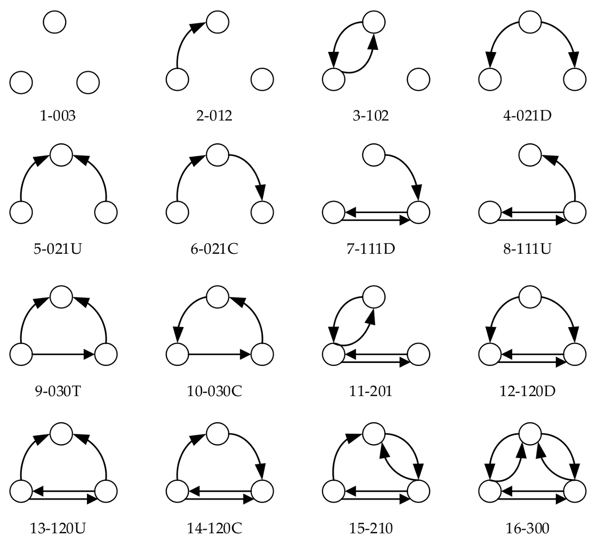
A pair of vertices and the lines between them is a dyad. Dyads fall into two categories: symmetric and asymmetric. A symmetric dyad means equivalence, a vertex is supposed to reciprocate the choices that it receives, while an asymmetric dyad signifies ranking, one vertex chooses the other but this choice is not reciprocated. Both mutual choices and mutual absent choices are symmetric. For analyzing the topological structure of a directed network, we proceed from dyads to triads and list 16 basic types of triads [29].

Triad type is identified by a M-A-N number of three digits, that is proposed by Davis, Holland, and Leinhardt [34]. The three digits respectively refer to the number of mutual positive dyads (M), the number of asymmetric dyads number (A), and the number of null dyads number (N). In triads with the same M-A-N digits, a letter is added to represent the direction of asymmetric choice: C for cyclic, U for Up, D for down, and T for transitive (Figure 2).

2.3. AQI Network Construction

To explore the AQI fluctuation with time, we transform the time series of the AQI into a directed-weighted network of the AQI.

2.3.1. Data Coarse-Grained Processing

The study object is the daily fluctuating information that rises or falls, so the AQI is coarsely grained at first to convert the continuous time series data into a wave state symbol sequence. The coarse-grained treatment is to discard the small details, break the original time series data into multiple finite sub-intervals, and use a character to represent the interval homogenization of subintervals. The symbol states are limited, which is more conducive to revealing the nature of AQI fluctuation. The accuracy of coarse-grained treatment determines the validity of the research conclusions, so there should not be too many symbol types, to be able to represent the stage characteristics of the AQI and be independent of each other.

Too much classification is not conducive to the discovery of wave patterns of AQI, therefore, according to fluctuation range (Formula (6)), the AQI data series is abstracted into three symbols H, M, and L, transformed into symbol sequence CS_i, as shown in

Table 2. Coarse-Grained processing of the AQI time series.

No	Date	City	AQI	Symbol
1	2013-11-1	Beijing	231	H
2	2013-11-2	Beijing	294	H
3	2013-11-3	Beijing	80	L
4	2013-11-4	Beijing	57	L
5	2013-11-5	Beijing	184	M
6	2013-11-6	Beijing	189	M
7	2013-11-7	Beijing	59	L
8	2013-11-8	Beijing	106	M
9	2013-11-9	Beijing	178	M
10	2013-11-10	Beijing	53	L
……	……	……	……	……
1448	2017-10-22	Beijing	54	L
1449	2017-10-23	Beijing	49	L
1450	2017-10-24	Beijing	90	L
1451	2017-10-25	Beijing	141	M
1452	2017-10-26	Beijing	195	M
1453	2017-10-27	Beijing	217	H
1454	2017-10-28	Beijing	78	L
1455	2017-10-29	Beijing	27	L
1456	2017-10-30	Beijing	40	L
1457	2017-10-31	Beijing	83	L

.

$$C{S}_i=\{\begin{array}{cc}H& AQI>200\\ M& 100<AQI\le 200\\ L& AQI\le 100,\end{array}$$

(6)

In Formula (6), the symbols H, M, and L respectively denote heavy or serious air pollution, mild or moderate air pollution and excellent or good air quality.

2.3.2. Definition of AQI Pattern

After the coarse-grained processing of the AQI, the time series data is transformed into the symbol sequence CS_t, which exhibits different rising or falling amplitudes of AQI. The time series and symbol sequence CS_t of AQI are equivalent. The symbol sequence CS_t is defined as follow.

$$C{S}_t = \left(c{s}_1, c{s}_2, c{s}_3, \dots , c{s}_n\right) \left(c{s}_i \in \left(H,M,L\right)\right)$$

(7)

A series of 1–10 symbols is individually regarded as one series, and the symbol sequence CS_t is transformed into AQI patterns through slide operation. The calculations reveal that a 6-symbols series as one pattern shows a stronger regularity (

Table 3. Pattern of different symbol series.

Symbol Series	Pattern Quantity	Growth Rate	Relative Growth Rate
1 symbols	3
2 symbols	9	200.00%
3 symbols	26	188.89%	−11.11%
4 symbols	72	176.92%	−11.97%
5 symbols	163	126.39%	−50.53%
6 symbols	292	79.14%	−47.25%
7 symbols	451	54.45%	−24.69%
8 symbols	624	38.36%	−16.09%
9 symbols	815	30.61%	−7.75%
10 symbols	998	22.45%	−8.15%

). Finally, 292 patterns are obtained from the symbol sequence CS_t via a 6-symbols series as one pattern. Each pattern evolves on the basis of the previous pattern, emerging with the characteristics of memorability and diversification.

The symbolic sequence CS_t should have 3⁶ = 729 wave patterns in theory, such as {LLLLLL, LLLLLM, MLLLLL, LLLLMM, LLLMMM, MMLLLL, MMMMMM, LMLLLL, LLMLLL, ……}, but only 292 patterns emerged in fact, and the other 437 patterns didn’t appear.

2.3.3. Construction of the AQI Directed-Weighted Network

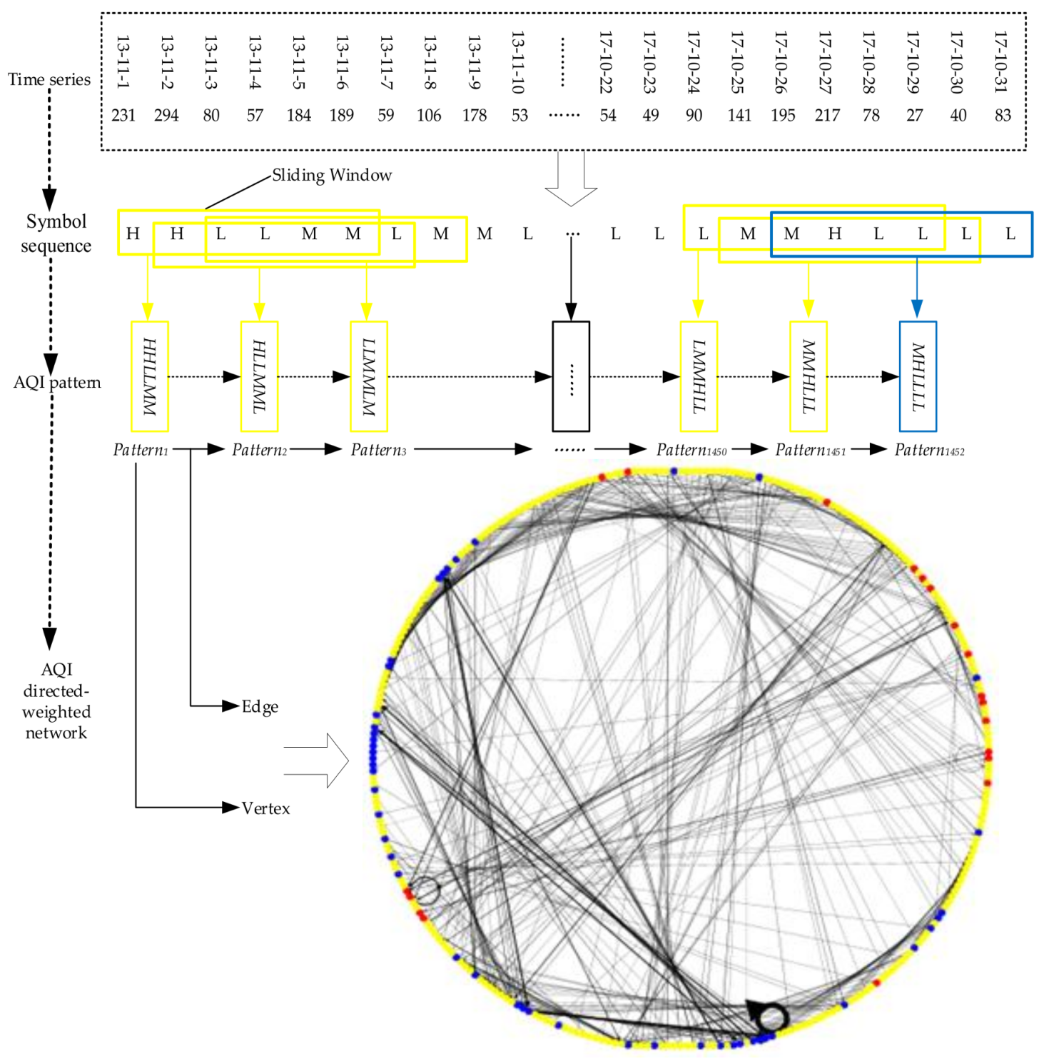
Each pattern is regarded as one vertex, the conversion among patterns is treated as one edge, finally, a directed-weighted network of the AQI is established. Edge (arrow) between vertices indicates the conversion direction, and edge size identifies the conversion frequency between patterns. In a directed-weighted network, the in-degree is the times other vertices are converted to current vertex, and out-degree is the times current vertex points to other vertices. Due to arcs between vertices being generated in a chronological order, the in-degree and out-degree of a vertex are equal (except the first and last vertex), so our study sets the number of received arcs as the edge weight of an AQI network. The entire modeling process is visualized in Figure 3.

In the AQI network, the vertex representing air pollution (H or M) lasting six days is set to red, the vertex representing air pollution (H or M) lasting 3–5 days is set to yellow, and the vertex representing air pollution (H or M) lasting 1–2 days is set to blue. Figure 3 shows that there are more conversion times and dense connection between vertices such as LLLLLL and LLLLLL, LLLLLL and LLLLLM, MMMMMM and MMMMMM, LLMMLL and LMMLLL.

3. Results and Analysis

3.1. Statistic Analysis

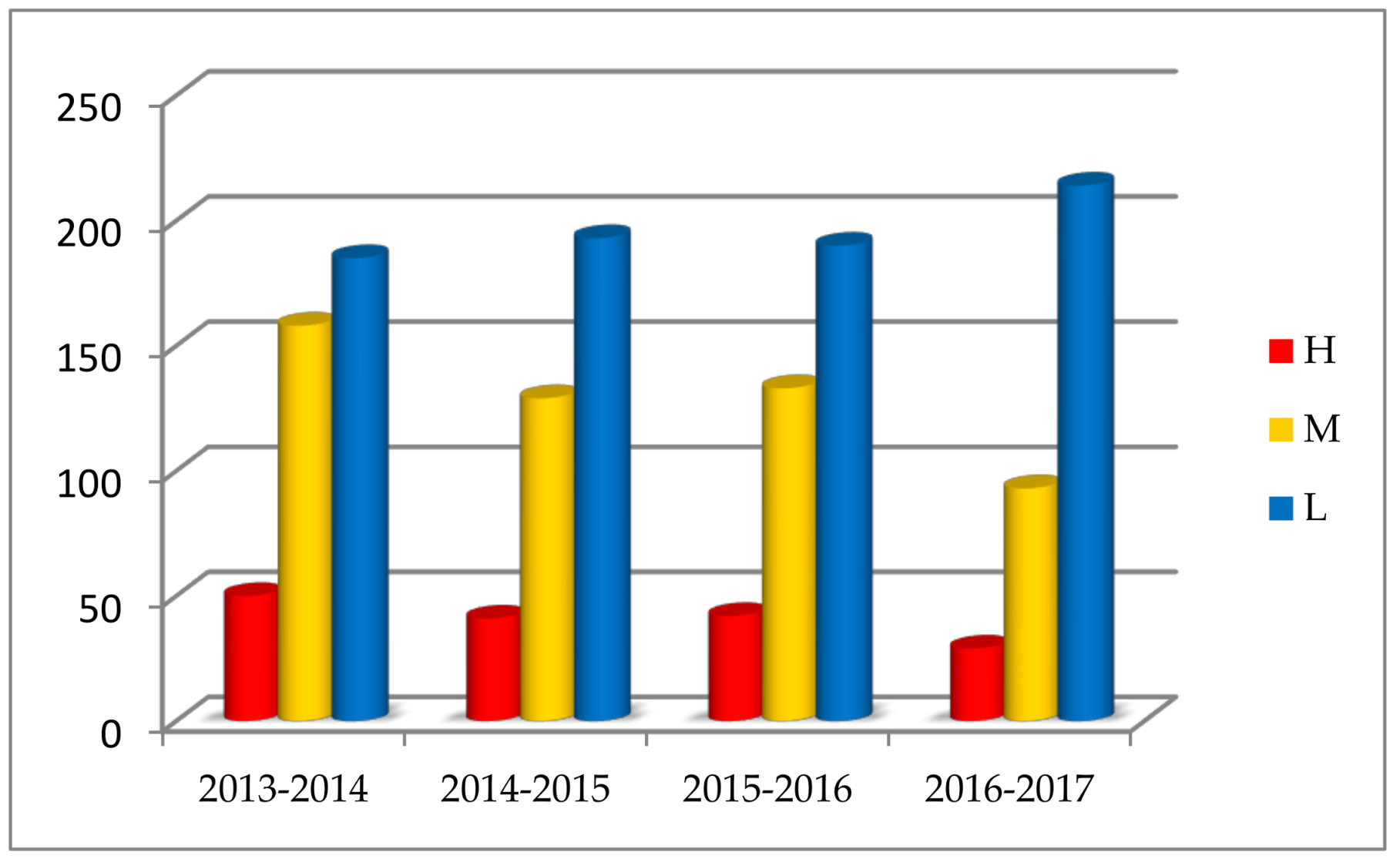
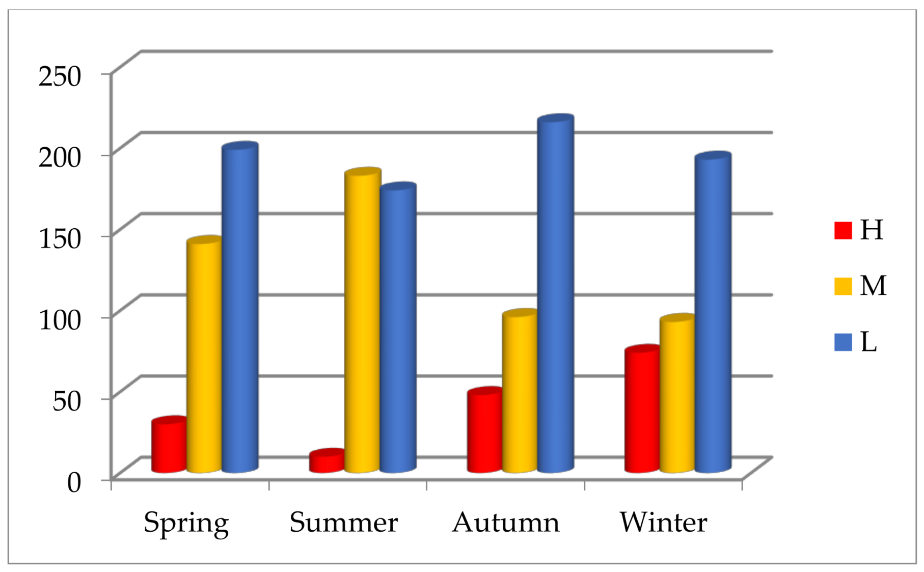
In the research duration, the statistics go through four years and four seasonal cycles. Among 1457 days in four years, the symbols H, M, and L respectively appear 162 times (11.12%), 513 times (35.21%), and 782 times (53.67%). Pollution days (H or M) in four years account for 46.33%, which indicates air pollution is serious in Beijing. From the annual statistics, the symbols H and M reduce, and the symbol L increases, which demonstrates that the overall air quality improves gradually in Beijing (Figure 4). From the seasonal statistics, heavy or serious air pollution (H) is most likely to occur in winter, mild or moderate air pollution (M) often appears in spring or summer, and the best air quality (L) recurs mostly in autumn (Figure 5).

3.2. Network Centrality Analysis

3.2.1. Vertex Strength

In AQI networks, the vertex strength represents the importance of the vertex, which indicates links received from other vertices. The larger the vertex strength is, the higher the vertex occurrence probability is, the more important the AQI pattern represented by vertex. Meanwhile, if a huge gap of vertex strength exists, the strength distribution will exhibit a “power-law” distribution, which means that a few vertices have a dominant effect in the AQI network.

The vertex strength and strength distribution of a directed-weighted network of the AQI in Beijing are calculated and shown in

Table 4. Vertex strength and distribution.

ID	Vertex	Vertex Strength	Strength Distribution
1	LLLLLL	127	8.75%
2	LLLLLM	57	3.93%
3	MLLLLL	51	3.51%
4	LLLLMM	41	2.82%
5	LLLMMM	34	2.34%
6	MMLLLL	34	2.34%
7	MMMMMM	34	2.34%
8	LMLLLL	29	2.00%
9	LLMLLL	28	1.93%
10	LLLMLL	25	1.72%
……	……	……	……
283	MMLHHM	1	0.69%
284	MMLHMM	1	0.69%
285	MMLLHH	1	0.69%
286	MMLLLH	1	0.69%
287	MMLMHH	1	0.69%
288	MMMHHL	1	0.69%
289	MMMHHM	1	0.69%
290	MMMHLL	1	0.69%
291	MMMLHH	1	0.69%
292	MMMLLH	1	0.69%

.

Table 4 illustrates the vertices LLLLLL, LLLLLM, and MLLLLL have maximum strength. The vertex strength of LLLLLL that means excellent or good air quality (AQI ≤ 100) lasting six days is 129, the strength distribution is only 8.7466%. However, the vertices that represent air pollution occurred at least one day in six days account for 91.2534%. The vertex strength and strength distribution of vertex HHHHHH that signifies heavy or serious air pollution (AQI > 200) lasting six days are seven and 0.4821%, whose vertex strength is ranked 46th in 292 vertices. The vertex strength and strength distribution of vertex MMMMM that indicates mild or moderate air pollution (100 < AQI ≤ 200) lasting six days are 34 and 2.3426%, whose vertex strength is ranked seventh in 292 vertices. These facts illustrate that the air pollution in Beijing is generally serious, but the best or worst air quality is rare, annd mild or moderate air pollution often occurs.

Sorted by vertex strength in descending order, among 292 vertices, the strength of the first 40 vertices is above eight, the strength distribution is above 0.5510%, and the cumulative strength distribution is 61.1570%. The strength of the first 20 vertices is above 16, the strength distribution is above 1.1019%, and the cumulative strength distribution is 45.5234%, which indicates the conversions of the AQI patterns frequently occur from the first 20 vertices to other vertices, or from other vertices to the first 20 vertices, or among 20 vertices. The strength distribution of the last 204 vertices is less than 0.25%, and the cumulative strength distribution is less than 20.6612%, which implies most AQI patterns represented by vertices rarely appear.

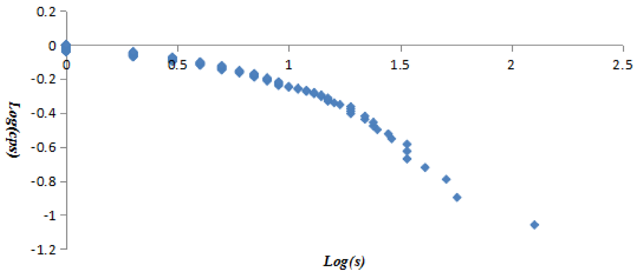
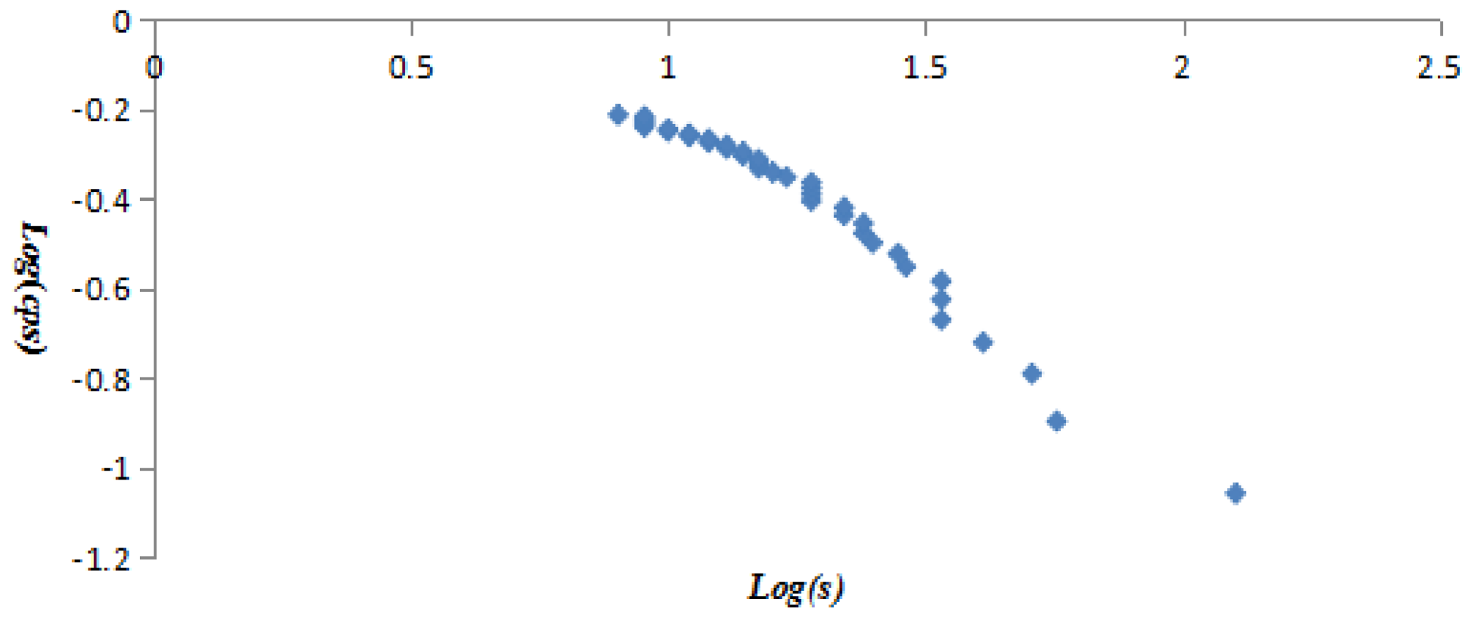
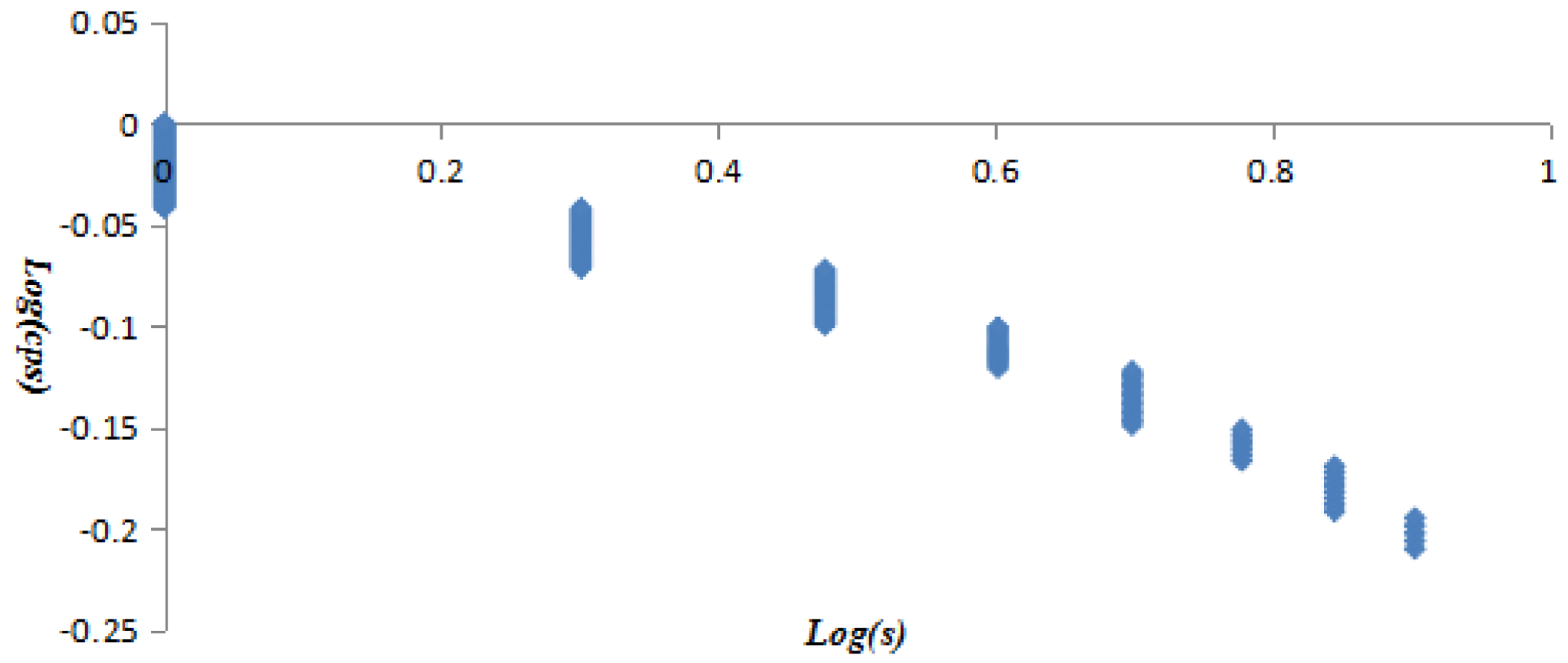
All vertices were listed in ascending order of vertex strength, the vertex strength and cumulative strength distribution (CSD) were treated with logarithmic function to get variables log(s) and log(csd), then taking log(s) and log(csd) as independent and dependent variables to establish the linear regression equation, and taking log(s) and log(csd) as X axis and Y axis to draw Figure 6. The obtained equation was y = −0.2996x + 0.0084 with R² = 0.8309. The equation and Figure 6 proved the vertex strength and cumulative strength distribution of the AQI network were in line with “power-law” distribution. Similarly, it was found that the vertex strength and cumulative strength distribution of the first 40 vertices (Figure 7) and the last 252 vertices (Figure 8) also conformed to the “power-law”. The linear regression equation of the first 40 vertices was y = −0.741x + 0.5205 with R² = 0.9592, and the linear regression equation of the last 252 vertices was y = −0.1682x − 0.01 with R² = 0.9259.

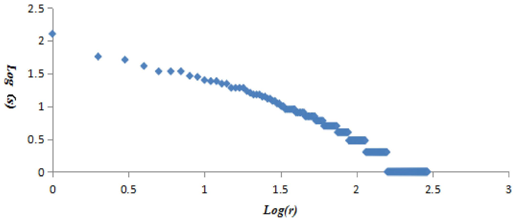
All vertices were presented in the descending order of vertex strength. The vertex strength and ranking were treated with logarithmic function to get variables log(s) and log(r), then log(s) and log(r) were regarded as dependent and independent variables to establish the linear regression equation. The obtained equation was y = −1.0504x + 2.5181 with R² = 0.9528. The results demonstrated the strengths and rankings of vertices in the AQI network also followed the “power-law” distribution (Figure 9).

The fact that vertex strength and cumulative strength distribution, and vertex strength and ranking all followed the “power-law” distribution proved that a few vertices played a leading role in the AQI network. Evidence from Table 4 showed that these hub vertices were LLLLLL, LLLLLM, MLLLLL, LLLLMM, LLLMMM, MMLLLL, MMMMMM, LMLLLL, LLMLLL, and LLLMLL; in particular, the AQI pattern MMMMMM has a larger vertex strength, which once again verified that air pollution in Beijing is mainly due to moderate pollution.

Long-term observation found that air pollution or excellent weather had persistent features, often lasting many days, so the weighted frequency W of n-same symbols series was calculated to analyze the pollution duration and level. The weighted frequency of the n-same symbols (H, M or L) series in the first 40 vertices had been calculated according to Formula (3), described below in

Table 5. The weighted frequency of the n-same symbols series.

Symbol Sequences	Weighted Frequency	Symbol Sequences	Weighted Frequency	Symbol Sequences	Weighted Frequency
H	0.07	M	1.22	L	2.36
HH	0.03	MM	0.60	LL	1.60
HHH	0.01	MMM	0.32	LLL	1.01
HHHH	0.00	MMMM	0.15	LLLL	0.55
HHHHH	0.00	MMMMM	0.07	LLLLL	0.26

. In the n-same symbols series, HHHHH means the probability that symbol H will last five days in six days, and the rest can be done in the same manner.

Table 5 shows that with the increase of the sequence length, the weighted frequency of the n-same symbols series decreases gradually. The weighted frequency of the n-same symbols series about L is the highest, which indicates the air quality in Beijing is dominated by excellent or good weather. The weighted frequency of the n-same symbols series about L and M is far above that of H, which demonstrates a mild or moderate level of air pollution (M) is more likely to occur than heavy or serious air pollution (H). The weighted frequencies of the same symbols series HHHH and HHHHH is 0, which indicates the probability of heavy or serious air pollution lasting for four or five days is very low, close to 0. The weighted frequency of same symbols series LLLLL is 0.26, which means there is a low probability of excellent or good air quality for five days. Overall, excellent or good weather dominates, but air pollution intermittently recurs in Beijing.

3.2.2. Closeness Centrality

In an AQI network, the weighted clustering coefficient quantifies the closeness degree between the vertex and its adjacent vertices. The larger the weighted clustering coefficient of one vertex, the more frequent and easy the conversion from an AQI pattern represented by this vertex to other AQI patterns.

The statistics notes that there are 17 vertices with a weighted clustering coefficient that is not 0, the vertices HHHHHL, HHHHHH, LLLLLL, and MMMMM possess a higher weighted clustering coefficient. The AQI patterns represented by them are closer than with others patterns; they convert to other patterns more frequently and easily. Particularly, the vertex MMMMM has both a larger vertex strength and weighted clustering coefficient, which means the AQI pattern moderate air pollution (M) lasting 6 days holds an important position in the AQI network (

Table 6. Weighted clustering coefficients of vertices.

ID	Vertex	Strength	Edges	Clustering Coefficient	Cumulative Percentage
1	HHHHHL	5	11	0.1515	12.15%
2	HHHHHH	7	7	0.1429	23.61%
3	LLLLLL	127	13	0.1026	31.84%
4	MMMMMM	34	7	0.0952	39.48%
5	LLLLLM	57	25	0.0800	45.89%
6	LLMLLM	6	11	0.0758	51.97%
7	MHHHHH	3	9	0.0741	57.91%
8	LHHHHH	3	7	0.0714	63.64%
9	MMLMML	3	11	0.0606	68.50%
10	MLLMLL	8	12	0.0556	72.96%
11	LMMLMM	5	12	0.0556	77.41%
12	MLMMLM	1	6	0.0556	81.87%
13	LMMMMM	15	13	0.0513	85.98%
14	MMMMML	12	14	0.0476	89.80%
15	LMLLML	1	7	0.0476	93.62%
16	HLLLLL	9	16	0.0417	96.96%
17	MLLLLL	51	22	0.0379	100.00%

).

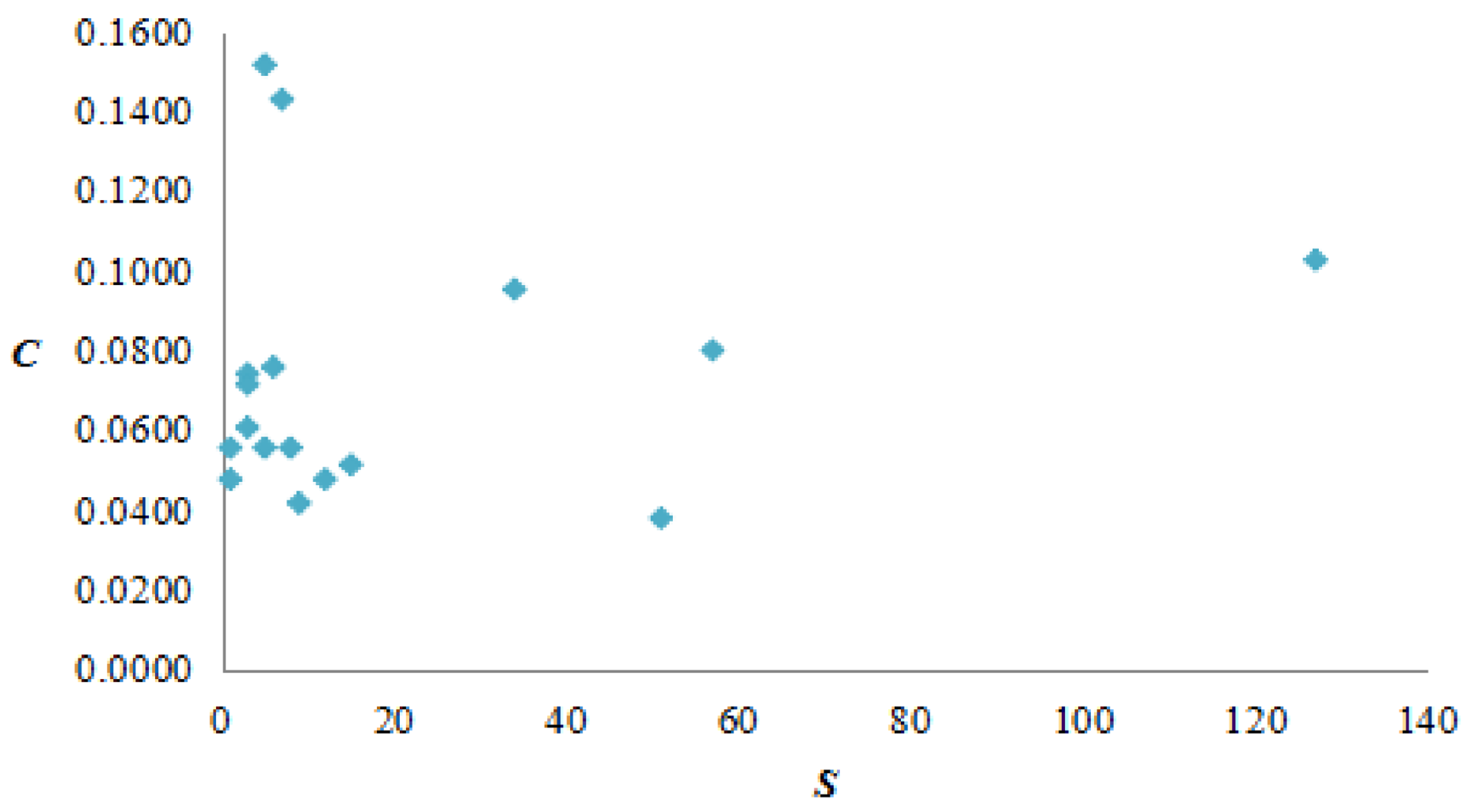
Taking the vertex strength and weighted clustering coefficient as the X coordinate and Y coordinate, it is found that the correlation between two variables is not strong, and the AQI network presents complicated polymorphism (Figure 10).

3.2.3. Betweenness Centrality

In an AQI network, the betweenness centrality of a vertex indicates the influence of the AQI pattern represented by this vertex as a communication hub, so controlling the intermediary vertex will cut off the path of air pollution diffusion. The betweenness centrality also helps to better understand the conversion process of AQI patterns, and provides a theoretical basis for formulating the treating measures of air pollution.

The betweenness centrality of each vertex in AQI network of Beijing was calculated and sorted in descending order, as shown in

Table 7. The vertex betweenness centrality in AQI network.

Node	Betweenness Centrality	Percent	Rank	Cumulative Betweenness Distribution
LLLMHH	0.1765	2.09%	1	2.09%
MLLLMM	0.1371	1.62%	2	3.71%
LLLLMH	0.1149	1.36%	3	5.06%
MLLLLM	0.1125	1.33%	4	6.39%
HLLLLM	0.1117	1.32%	5	7.71%
LLLLMM	0.1085	1.28%	6	8.99%
LMLLLM	0.1058	1.25%	7	10.25%
LLLMMM	0.1025	1.21%	8	11.46%
MMLLLL	0.1002	1.18%	9	12.64%
LLLMMH	0.0945	1.12%	10	13.76%
……	……	……	……	……
LMLMMH	0.0046	0.05%	283	99.73%
MLMMHH	0.0046	0.05%	284	99.79%
HMMMML	0.0043	0.05%	285	99.84%
HHHHHM	0.0034	0.04%	286	99.88%
LMLLML	0.0032	0.04%	287	99.92%
HMLLML	0.0029	0.03%	288	99.95%
MMLMLM	0.0023	0.03%	289	99.98%
MLMMLM	0.0011	0.01%	290	99.99%
HMMMMH	0.0008	0.01%	291	100.00%
HHHHHH	0.0000	0.00%	292	100.00%

.

The vertex with highest betweenness centrality is LLLMHH, followed by MLLLMM, LLLLMH, MLLLLM, HLLLLM, LLLLMM, LMLLLM, LLLMMM, MMLLLL, and LLLMMH. It is observed that the intermediary of every vertex is not strong. The betweenness centralization of the whole AQI network is 14.80%, indicating the AQI network does not have an obvious central tendency towards intermediaries. It is difficult to control the spread of air pollution by controlling some intermediary vertices.

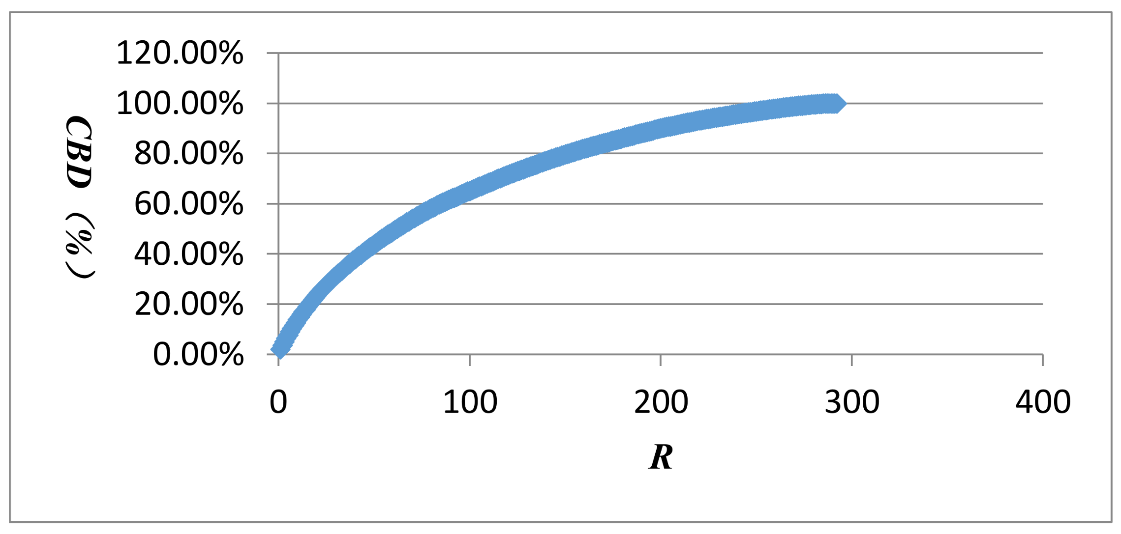
The cumulative distribution curve of betweenness centrality appears in Figure 11, which demonstrates that the slope is not steep, and the overall distribution of betweenness centrality is uniform. While the slope decreases gradually in the back, the varieties in the intermediation of the vertices still exist. Statistics also lends evidence that the cumulative distribution of the top 60 vertices reaches 49.09%, indicating that 20.55% of vertices account for nearly 1/2 of the intermediaries in the AQI network. Paying attention to these vertices and taking actions to control them will have great significance in preventing the diffusion of air pollution.

3.3. Structural Clusterability Analysis

The clusterability analysis will reveal how many clusters exist in the AQI network, and which AQI patterns often appear together. The multiple edges are more institutional and less personal, so we use island analysis technology to explore network clusters. When minimum island size is set to two, and maximum island size is set to 291, the vertices of the AQI network fall into six islands (

Table 8. Frequency distribution of cluster values.

Cluster	Freq	Freq%	CumFreq	CumFreq%	Representative
0	149	51.0274	149	51.0274	HHHHHM
1	2	0.6849	151	51.7123	LLLHHL
2	132	45.2055	283	96.9178	HHHHHH
3	2	0.6849	285	97.6027	LHHLLL
4	2	0.6849	287	98.2877	HHHHML
5	3	1.0274	290	99.3151	HHLMLM
6	2	0.6849	292	100.0000	LMHLLL

).

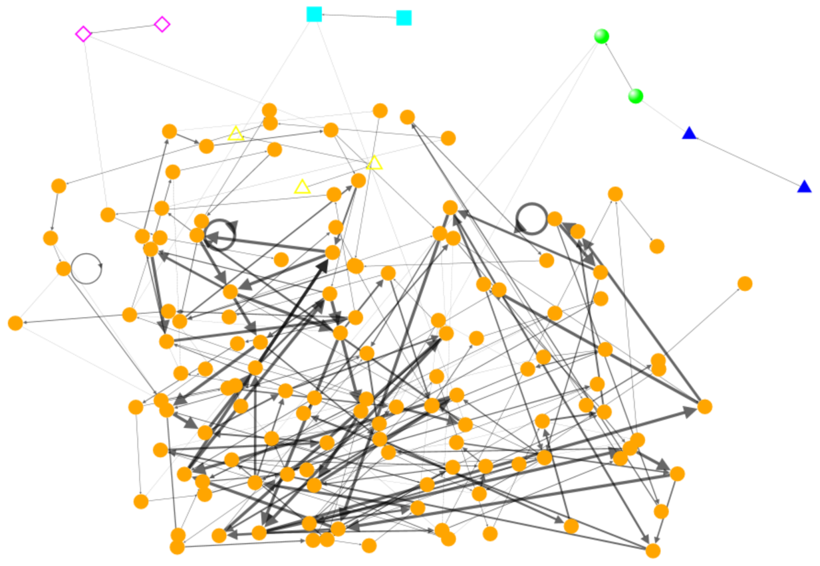
In Table 8, island 0 represented by HHHHHM means the corresponding vertices do not belong to any category. Islands 1, 3, 4, 6 are respectively represented by LLLHHL, LHHLLL, HHHHML, LMHLLL, and only contain two vertices. Island 5 contains three vertices. However, island 2 represented by HHHHHH contains 132 vertices, which reveals AQI pattern HHHHHH—meaning heavy or serious air pollution lasting six days—is very cohesive; many AQI patterns emerge around it, which once again proves that the air pollution in Beijing is very serious, and, more significantly, that heavy or serious air pollution always lingers for a long time.

Figure 12 visually exhibits the six islands of the AQI network. It is found that island 2 is the largest one; more connections between vertices occur in the same island, but fewer in different islands, and the more multiple connections, the thicker the line.

3.4. Structural Ranking Analysis

3.4.1. Prestige

The vertex with a higher ranking receives many choices from other vertices, so the AQI pattern represented by it tends to be an endpoint or residential location in the air pollution diffusion process. On the contrary, one vertex with a lower ranking is often a starting point or a transit point in the air pollution diffusion process.

As shown in

Table 9. The in-degree, input domain, and proximity prestige of vertex.

ID	Vertex	In-Degree	Input Domain	Mean Distance	Proximity Prestige
105	LLLLMH	3	291	6.1203	0.1634
107	LLLLMM	3	291	6.1237	0.1633
110	LLLMLL	3	291	6.1443	0.1628
104	LLLLLM	3	291	6.1684	0.1621
113	LLLMML	3	291	6.1718	0.1620
103	LLLLLL	3	291	6.1856	0.1617
221	MLLLLL	3	291	6.3127	0.1584
222	MLLLLM	3	291	6.3162	0.1583
112	LLLMMH	2	291	6.4192	0.1558
114	LLLMMM	2	291	6.4227	0.1557
……	……	……	……	……	……
143	LMHLMH	1	291	14.8557	0.0673
214	MLHMLL	1	291	14.9656	0.0668
70	HMMLML	1	291	15.0069	0.0666
211	MLHHHL	1	291	15.2749	0.0655
55	HMLHLL	1	291	15.7938	0.0633
200	MHLMHL	1	291	15.7973	0.0633
77	LHHHLL	1	291	16.2268	0.0616
213	MLHLLL	1	291	16.7354	0.0598
45	HLMHLL	1	291	16.7388	0.0597
81	LHLLLM	1	291	17.6770	0.0566

, the AQI network is a fully connected network, and the input domain of each vertex contains all other vertices (291), so the proximity prestige is equal to the inverse of the mean distance.

Table 10. The statistics of mean distance from input domain.

Vector Values	Frequency	Freq%	CumFreq	CumFreq%
1–6.120	0	0.0000	0	0.0000
6.120–9.973	200	68.4932	200	68.4932
9.973–13.825	74	25.3425	274	93.8356
13.825–17.677	18	6.1644	292	100.0000

reveals the mean distance of 68.4932% vertices is 6.120–9.973, which reveals the AQI network does not have obvious small-world phenomena, and the conversion of AQI patterns presents the characteristics of periodicity and regularity.

Table 11. The Statistics of Proximity Prestige.

Vector Values	Frequency	Freq%	CumFreq	CumFreq%
0–0.057	0	0.0000	0	0.0000
0.057–0.092	59	20.2055	59	20.2055
0.092–0.128	169	57.8767	228	78.0822
0.128–0.163	64	21.9178	292	100.0000

illustrates that 64 (21.9178%) vertices have higher proximity prestige and shorter mean distance with other vertices. AQI patterns represented by them stay a long time in the AQI fluctuation process, dominating the diffusion of air pollution.

3.4.2. Triadic Analysis

The triad census of the AQI network is compared with the chance distribution of triad types; if several triad types of AQI network occur more frequently than expected by chance, the corresponding triad type may guide or influence the structure of AQI network. When the number of forbidden triads is less than expected by chance, balance theory could be used to explain network structure, which divides the network types into balance, cluster ability, ranked clustering, transitivity, or hierarchical clusters.

Table 12. The triadic census of AQI network in Beijing.

Type	Number of Triads(ni)	Expected(ei)	(ni-ei)/ei	Model
3-102	0	335.32	−1.00	Balance
16-300	0	0.00	−1.00	Balance
1-003	3,978,206	3,978,760.46	−0.00	Clusterability
4-021D	182	335.32	−0.46	Ranked Clusters
5-021U	184	335.32	−0.45	Ranked Clusters
9-030T	5	3.55	0.41	Ranked Clusters
12-120D	0	0.01	−1.00	Ranked Clusters
13-120U	0	0.01	−1.00	Ranked Clusters
2-012	127,635	126,531.02	0.01	Transitivity
14-120C	0	0.02	−1.00	Hierarchical Clusters
15-210	0	0.00	−1.00	Hierarchical Clusters
6-021C	766	670.65	0.14	Forbidden
7-111D	0	3.55	−1.00	Forbidden
8-111U	0	3.55	−1.00	Forbidden
10-030C	2	1.18	0.69	Forbidden
11-201	0	0.01	−1.00	Forbidden

Node: Chi-Square: 505.2910 ***, 10 cells (62.50%) have expected frequencies less than 5. The minimum expected cell frequency is 0.00.

indicates that the chi-square statistic is statistically significant at the 0.001 level, and the AQI network is clearly different from that random network. The frequency of three in five forbidden triads (7-111D, 8-111U, 11-201) is less than expected by chance. Two triads (2-012, 9-030T) are expected to occur more often than by chance, thereinto the number of triads 2-012 is 127635, appearing substantially more often than the chance-expected number 126,531.02, so a transitivity model seems to be the best choice for the AQI network. However, many other triads (300, 16-300, 1-003, 4-021D, 5-021U, 12-120D, 13-120U, 14-120C, 15-210) appear less than expected by chance. This casts some doubt on the reliability of the chi-square measure.

4. Conclusions and Discussion

This study converted time series data into a symbol sequence through the coarse graining process; established the directed-weighted network of the AQI; then analyzed the centrality, clusterability, and ranking of the AQI network. The main results and conclusions are summarized as follows.

The statistics show that air pollution in Beijing is serious, but air quality improves gradually. The AQI in Beijing has seasonal variations; heavy or serious air pollution mostly recurs in winter, and the excellent or good air quality often appears in autumn. The statistical results are consistent with the subjective experience, perhaps because the meteorological conditions of autumn in Beijing are better and favorable for the diffusion of air pollutants.

The vertex strength and cumulative strength distribution, and vertex strength and ranking follow “power-law” distribution; the AQI network is a scale-free network, which means only a few AQI patterns—represented by so-called super vertices which play a leading role in the AQI network—appear frequently. The best or worst air quality in Beijing is rare; mild or moderate air pollution often occurs. The probability of heavy or serious air pollution lasting for 4 or 5 days is very low, close to 0.

17 vertices have a weighted clustering coefficient greater than 0. The vertex MMMMM has both larger vertex strength and weighted clustering coefficient, holding an important position in the AQI network. The correlation between vertex strength and weighted clustering coefficient is not strong and the AQI network presented complicated polymorphism.

The AQI network does not have an obvious central tendency towards intermediaries, but the varieties in the intermediation of the vertices still exist; 20.55% of vertices account for nearly ½ of the intermediaries in the AQI network. It is difficult to restrain the diffusion of air pollution by controlling the intermediate vertex, but it is also possible.

The vertices of the AQI network fall into six islands; the largest island represented by HHHHHH contains 132 vertices, which means the AQI pattern of heavy or serious air pollution lasting six days is very cohesive, always lingering for a long time.

The AQI network is a fully connected network, which does not have obvious small-world phenomena; the mean distance of 68.4932% vertices is 6.120–9.973, and the conversion of AQI patterns presents the characteristics of periodicity and regularity. The 64 vertices had high proximity prestige and dominated the AQI network. They are often the endpoints or residential locations in the air pollution diffusion process, dominating the diffusion of air pollution. The number of triads 2-012 is the largest, and the AQI network seems to follow the transitivity model, however, many other triads appear less than expected by chance, which casts some doubt on the reliability of the chi-square measure.

Air pollution is one essential environmental problem. Our study firstly applies complex network theory to analyze the AQI, and reveals the AQI fluctuation law and internal mechanism, which can provide evidence for formulating the countermeasures about preventing and controlling air pollution. Meanwhile, our study also presents a new approach for time series prediction, contributing to existing studies. In different areas and times, air quality is affected by different factors, such as atmospheric conditions, fossil fuel emissions, landform features, and measures for prevention and control of pollution. Although revealing the topological properties hidden behind the AQI time series, this study does not analyze the factors that lead to the change of air quality. Constructing an influence factors model to reveal the causes of AQI pattern variety in different times is the research direction and content for the future.

References

- Kampa, M.; Castanas, E. Human health effects of air pollution. Environ. Pollut. 2008, 151, 362–367. [Google Scholar] [CrossRef] [PubMed]
- Cole-Hunter, T.; de Nazelle, A.; Donaire-Gonzalez, D.; Kubesch, N.; Carrasco-Turigas, G.; Matt, F.; Martinez, D. Estimated effects of air pollution and space-time-activity on cardiopulmonary outcomes in healthy adults: A repeated measures study. Environ. Int. 2018, 111, 247–259. [Google Scholar] [CrossRef] [PubMed]
- Cohen, A.J.; Brauer, M.; Burnett, R.; Anderson, H.R.; Frostad, J.; Estep, K.; Feigin, V. Estimates and 25-year trends of the global burden of disease attributable to ambient air pollution: An analysis of data from the Global Burden of Diseases Study 2015. Lancet 2017, 389, 1907–1918. [Google Scholar] [CrossRef]
- Chen, X.; Shao, S.; Tian, Z.; Xie, Z.; Yin, P. Impacts of air pollution and its spatial spillover effect on public health based on China’s big data sample. J. Clean. Prod. 2017, 142, 915–925. [Google Scholar] [CrossRef]
- Yale Center for Environmental Law and Policy, International Earth Science Information Network(CIESIN). 2016 Environmental Performance Index [OL]. Available online: http://epi.yale.edu (accessed on 28 January 2016).
- Zhou, X.; Cao, Z.; Ma, Y.; Wang, L.; Wu, R.; Wang, W. Concentrations, correlations and chemical species of PM2.5/PM10 based on published data in China: Potential implications for the revised particulate standard. Chemosphere 2016, 144, 518–526. [Google Scholar] [CrossRef] [PubMed]
- Zhu, S.; Lian, X.; Liu, H.; Hu, J.; Wang, Y.; Che, J. Daily air quality index forecasting with hybrid models: A case in China. Environ. Pollut. 2017, 231, 1232–1244. [Google Scholar] [CrossRef] [PubMed]
- Wang, D.; Wei, S.; Luo, H.; Yue, C.; Grunder, O. A novel hybrid model for air quality index forecasting based on two-phase decomposition technique and modified extreme learning machine. Sci. Total Environ. 2017, 580, 719–733. [Google Scholar] [CrossRef] [PubMed]
- Song, Y.; Qin, S.; Qu, J.; Liu, F. The forecasting research of early warning systems for atmospheric pollutants: A case in Yangtze River Delta region. Atmos. Environ. 2015, 118, 58–69. [Google Scholar] [CrossRef]
- Rahman, N.H.A.; Lee, M.H.; Latif, M.T. Artificial neural networks and fuzzy time series forecasting: An application to air quality. Qual. Quant. 2015, 49, 2633–2647. [Google Scholar] [CrossRef]
- Zhou, Q.; Jiang, H.; Wang, J.; Zhou, J. A hybrid model for PM2. 5 forecasting based on ensemble empirical mode decomposition and a general regression neural network. Sci. Total Environ. 2014, 496, 264–274. [Google Scholar] [CrossRef] [PubMed]
- Goyal, P.; Chan, A.T.; Jaiswal, N. Statistical models for the prediction of respirable suspended particulate matter in urban cities. Atmos. Environ. 2006, 40, 2068–2077. [Google Scholar] [CrossRef]
- Hua, Z.; Wang, Y.; Xu, X.; Zhang, B.; Liang, L. Predicting corporate financial distress based on integration of support vector machine and logistic regression. Expert Syst. Appl. 2007, 33, 434–440. [Google Scholar] [CrossRef]
- Liu, B.C.; Binaykia, A.; Chang, P.C.; Tiwari, M.K.; Tsao, C.C. Urban air quality forecasting based on multi-dimensional collaborative support vector regression (SVR): A case study of Beijing-Tianjin-Shijiazhuang. PLoS ONE 2017, 12, e0179763. [Google Scholar] [CrossRef] [PubMed]
- Mishra, D.; Goyal, P. Neuro-fuzzy approach to forecast NO2 pollutants addressed to air quality dispersion model over Delhi, India. Aerosol Air Qual. Res. 2016, 16, 166–174. [Google Scholar] [CrossRef]
- Liu, Y.; Zhu, Q.; Yao, D.; Xu, W. Forecasting urban air quality via a back-propagation neural network and a selection sample rule. Atmosphere 2015, 6, 891–907. [Google Scholar] [CrossRef]
- Kumar, A.; Goyal, P. Forecasting of air quality index in delhi using neural network based on principal component analysis. Pure Appl. Geophys. 2013, 170, 711–722. [Google Scholar] [CrossRef]
- Tamas, W.; Notton, G.; Paoli, C.; Nivet, M.L.; Voyant, C. Hybridization of air quality forecasting models using machine learning and clustering: An original approach to detect pollutant peaks. Aerosol Air Qual. Res. 2016, 16, 405–416. [Google Scholar] [CrossRef]
- Jiang, J.L.; Su, X.; Zhang, H.; Zhang, X.H.; Yuan, Y.J. A novel approach to active compounds identification based on support vector regression model and mean impact value. Chem. Biol. Drug Des. 2013, 81, 650–657. [Google Scholar] [CrossRef] [PubMed]
- Ortiz-García, E.G.; Salcedo-Sanz, S.; Pérez-Bellido, Á.M.; Portilla-Figueras, J.A.; Prieto, L. Prediction of hourly O3 concentrations using support vector regression algorithms. Atmos. Environ. 2010, 44, 4481–4488. [Google Scholar] [CrossRef]
- Lu, W.Z.; Wang, D. Ground-level ozone prediction by support vector machine approach with a cost-sensitive classification scheme. Sci. Total Environ. 2008, 395, 109–116. [Google Scholar] [CrossRef] [PubMed]
- Collins, J.M.; Clark, M.R. An application of the theory of neural computation to the prediction of workplace behavior: An illustration and assessment of network analysis. Pers. Psychol. 1993, 46, 503–524. [Google Scholar] [CrossRef]
- Wang, P.; Liu, Y.; Qin, Z.; Zhang, G. A novel hybrid forecasting model for PM10 and SO2 daily concentrations. Sci. Total Environ. 2015, 505, 1202–1212. [Google Scholar] [CrossRef] [PubMed]
- De Mattos Neto, P.S.; Madeiro, F.; Ferreira, T.A.; Cavalcanti, G.D. Hybrid intelligent system for air quality forecasting using phase adjustment. Eng. Appl. Artif. Intell. 2014, 32, 185–191. [Google Scholar] [CrossRef]
- Gao, X.Y.; An, H.Z.; Liu, H.H.; Ding, Y.H. Analysis on the topological properties of the linkage complex network between crude oil future price and spot price. Acta Phys. Sin. 2011, 60, 068902. [Google Scholar]
- Wan, L.; Shu, K.; Guo, Y. Communications and Information Processing: Sequences Modeling and Analysis Based on Complex Network; Springer: Berlin/Heidelberg, Germany, 2012. [Google Scholar]
- Zhou, L.; Gong, Z.Q.; Zhi, R.; Feng, G.L. Approach to research the topology of Chinese temperature sequence based on complex network. Acta Phys. Sin. 2008, 57, 7380–7389. [Google Scholar]
- Lewis, T.G. Network Science: Theory and Applications; John Wiley & Sons: Hoboken, NJ, USA, 2011. [Google Scholar]
- De Nooy, W.; Mrvar, A.; Batagelj, V. Exploratory Social Network Analysis with Pajek; Cambridge University Press: Cambridge, UK, 2011. [Google Scholar]
- Watts, D.J.; Strogatz, S.H. Collective dynamics of ‘small-world’ networks. Nature 1998, 393, 440–442. [Google Scholar] [CrossRef] [PubMed]
- Onnela, J.P.; Saramäki, J.; Kertész, J.; Kaski, K. Intensity and coherence of motifs in weighted complex networks. Phys. Rev. E 2005, 71, 065103. [Google Scholar] [CrossRef] [PubMed]
- Holme, P.; Park, S.M.; Kim, B.J.; Edling, C.R. Korean university life in a network perspective: Dynamics of a large affiliation network. Phys. A Stat. Mech. Appl. 2007, 373, 821–830. [Google Scholar] [CrossRef]
- Scott, J.; Hughes, M. The Anatomy of Scottish Capital: Scottish Companies and Scottish Capital, 1900–1979; Croom Helm: Kent, UK, 1980; Volume 33. [Google Scholar]
- Davis, J.A. The davis/holland/leinhardt studies: An overview. In Perspectives Social Network Research; Holland, P.W., Leinhardt, S., Eds.; Academic Press: New York, NY, USA, 1979. [Google Scholar]
Figure 1.
The time series of air quality index (AQI) in Beijing.
Figure 2.
The basic triad types in a directed network.
Figure 3.
The construction process of an AQI directed-weighted network.
Figure 4.
The annual proportion of AQI symbols in Beijing.
Figure 5.
The seasonal proportion of AQI symbols in Beijing.
Figure 6.
The log–log plots of vertex strength and cumulative strength distribution.
Figure 7.
The log–log plots of vertex strength and cumulative strength distribution of the first 40 vertices.
Figure 8.
The log–log plots of vertex strength and cumulative strength distribution of the last 252 vertices.
Figure 9.
The log–log plots of vertex strength and ranking.
Figure 10.
Vertex strength and weighted clustering coefficient.
Figure 11.
The cumulative betweenness distribution of betweenness centrality.
Figure 12.
The island analysis of the AQI network.