1. Introduction
The urbanization process in China is complex, as it commenced later but is progressing faster than in other countries [
1]. The impetus was the economic reform of China, after which the process accelerated and deepened. According to the National Development and Reform Commission [
2], China’s level of urbanization increased substantially in the 30 years since its reform and opening up. Between 1978 and 2010, the urban population increased from 17.9 to 49.68% of the total population, or from 170 to 665.57 million people, representing an average annual increase of 15.839 million. China’s population became 30% urban in 1996 and exceeded 50% urban (51.27%) for the first time in 2011, further increasing to 54.77% by 2014. Northam [
3] posited an “S” curve of urbanization, with three stages: slow growth in urbanization when urban population is less than 30%; accelerated development when urban population is 30–70%; and maturation and stability following slowing urbanization at 70%. In terms of this curve, China can be considered to be in the second stage, rapid urbanization, as its urbanization level is still lower than 70%. Rural-urban and regional disparities in the country are large, but the internal momentum for further urbanization remains strong.
Wei and Ye [
4] indicate that during the urbanization process of China land use and environmental issues are important in term of sustainability of Chinese cities. Gao et al. [
5] analyze urban land expansion and structural changes in the Yangtze River Delta (YRD) and find that cities in the YRD are experiencing urban land expansion mainly characterized by the growth of residential and industrial land. Qian et al. [
6] introduce the evolution of urban land expansion and the sustainable land use policy of the Shenzhen Government since 2005. They find that the current top-down indicative and mandatory mode of control, which relies on the central government, has very limited effects. Wan et al. [
7] evaluate the level of urbanization and analyzes the relationship between the level of urbanization and ecosystem service values in Huaibei, China. They find that Huaibei’s level of urbanization has progressed gradually during the study period while ecosystem service values increased at the earlier time period but dropped in later time. Based on the method provided by the IPCC, Cheng et al. [
8] examine the spatiotemporal dynamics and dominating factors of China’s carbon intensity from energy consumption in 1997–2010. The results show that energy intensity, energy structure, industrial structure and urbanization rate are the dominating factors shaping the spatiotemporal patterns of China’s carbon intensity from energy consumption.
One of the issues that cities face during the process of urbanization is spatial mismatch. John Kain [
9] proposes the hypothesis of spatial mismatch, which states that mismatches between occupational and living spaces cause various issues including unemployment among vulnerable groups and excessive commuting time [
10,
11,
12,
13]. In the case of China, Wang et al. [
14] show that in the Yangtze River Delta, the speed and scale of the movement of regional economic centers have far exceeded shifts in the population centers. This has resulted in uneven distribution of population and economic activities. Zhou et al. [
15] measure spatial match between population and economic activities in Chongqing over 40 years. They identify that consistency between the two variables was closely related to various factors including natural conditions, regional positioning, imbalances in regional development, and changes in industrial structure. Spatial mismatch of economic elements means that elements must be transported on a large scale over long distances and undergo large amounts of intermediate wear during the process [
16,
17]. The mismatch of industrial and occupational spaces means that there is inequality in employment opportunities: areas where industries cluster have adequate job supplies and low unemployment rates, while other areas with less industrial activities but higher population suffer from a relative lack of jobs and an unemployment problem [
18,
19]. Spatial mismatch between the economy and population causes a distortion between residence and employment, leading to issues of traffic congestion and soaring housing prices with urbanization [
20,
21]. Keith Ihlanfeldt [
22] indicates that policy options to the spatial mismatch problem can be classified into two categories: (1) policies to reduce distances between the residential locations of minorities and the locations of available jobs, and (2) policies to improve the job accessibility of minorities, without changing either job or residential locations.
Another outcome of rapid urbanization has been a significant growth in urban residential carbon emissions [
23,
24,
25,
26]. At present, urban residences, transportation, and industries are the three main areas of energy consumption in China. Residential energy consumption accounted for 10% of total energy consumption in 1978, but has since risen to 27.5%. This proportion is likely to continue growing due to the country’s increasing rate of urbanization. This will result in sustained increases in carbon emissions, making the reduction of emissions an important issue in the effort to promote low-carbon urbanization in China [
27,
28].
The Intergovernmental Panel on Climate Change (IPCC) is the premier organization developing methods to estimate GHG emissions. The 2006 IPCC Guidelines contain the latest, scientifically robust and internationally accepted methods for estimating GHG inventories [
29]. The IPCC Guidelines also outline the preeminent methods for estimating residential carbon dioxide emissions in terms of the species which are emitted. During the combustion process, most carbon is immediately emitted as CO
2. So IPCC Guidelines provide default emission factors for CO
2 that are applicable to all combustion processes, both stationary and mobile. Such CO
2 emission factors for fuel combustion are relatively insensitive to the combustion process itself but are primarily dependent only on the carbon content of the fuel.
The traditional method is to use macroscopic statistical data on energy consumption and determine emissions with a conversion coefficient [
26,
30]. The data required for this method are easily obtainable and have temporal continuity, which facilitates comparisons between different regions or time periods. Although widely used, it is limited by statistical resolution and cannot reflect the heterogeneity within areas undergoing rapid urbanization. Alternatively, some scholars have conducted field research at smaller scale with a large sample size to understand the spatial characteristics and formation mechanisms of residential carbon emissions [
31,
32]. Although this approach provides accurate spatial attributes for analysis, substantial inputs are needed to obtain data continuity, which prevents its widespread adoption.
Recently, some researchers have begun to study carbon emissions using new data sources based on monitoring of human activities [
33,
34,
35,
36]. Among these, the remote sensing data of the Defense Meteorological Satellite Program Operational Linescan System (DMSP/OLS) portray the spatial patterns of human activities in urban areas live, fast, and continuously, leading to the widespread application of this data [
37,
38,
39]. The first global map of CO
2 emissions has a spatial resolution of 1 degree and is developed by combining the lighted area of a city (using imagery of nighttime lights acquired between October 1994 and March 1995) with country-level ancillary statistical information [
40]. Oda and Maksyutov [
41] create a high resolution global inventory of annual CO
2 emissions for the years 1980–2007 by combining a worldwide point source database with satellite observations of global nighttime lights distribution. Ghosh et al. [
35] develop a method of mapping spatially distributed CO
2 emissions from the burning of fossil fuels (excluding electric power utilities) at 30 arc-seconds (approximately 1 km
2 resolution) using regression models of nighttime lights images. More recently, Lu and Liu [
42] present a novel method that utilizes spatially distributed information from nighttime lights and human activity index to test the hypothesis that counties with similar carbon dioxide emissions from residential carbon dioxide emissions are more spatially clustered than would be expected by chance. Wang and Liu [
43] examine the spatiotemporal variations and determinants of CO
2 emissions using a series of distribution dynamic approaches and panel data models for proposing feasible mitigation policies, the results of which show that while per capital CO
2 emissions were characterized by significant regional inequalities and self-reinforcing agglomeration during the study period, regional disparities decreased and spatial agglomeration gradually increased between 1992 and 2013.
The aim of this study was to examine the spatial match and/or mismatch between carbon emissions and economic activities. This was achieved by constructing a spatial model of carbon emissions based on night-time light, which was applied to understand the spatial pattern of emissions in Zhengzhou City, which is undergoing rapid urbanization. Transport emissions are important in cities emissions. However, we did not include transport emissions for the following reasons: (1) The carbon emissions map produced by night-time lights is an image with resolutions of around 1 km per pixel. Since it is very larger than road night-time lights can’t measure the transport emissions; (2) We tried to use other sources (statistical data of Zhengzhou) to estimate transport emissions. However statistical data can only produce very low spatial resolution map. Such huge difference of two spatial resolutions prevented us to include transport emissions in study of spatial mismatch. As a result, this study mainly focused on carbon emissions in residential building areas.
2. Research Area
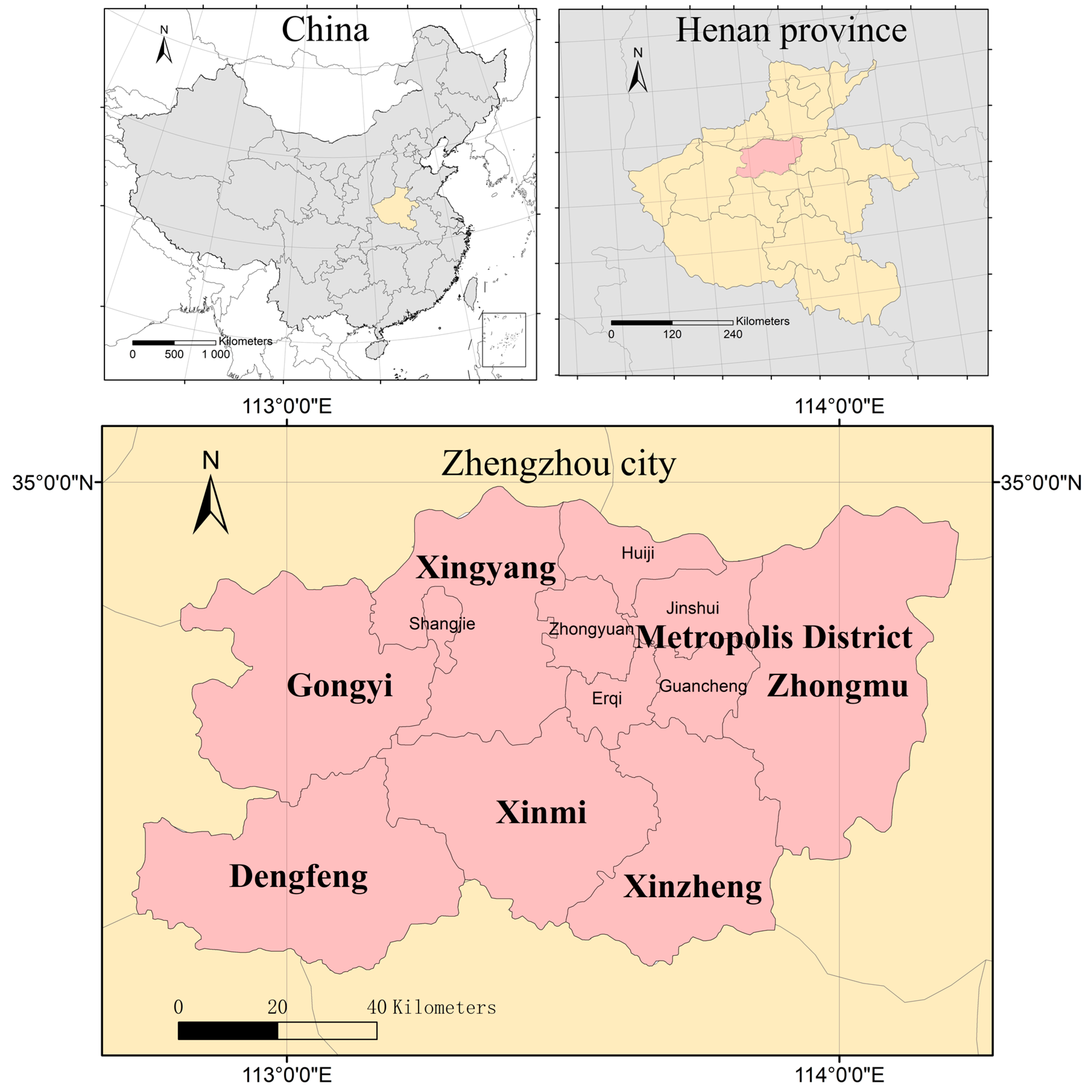
Zhengzhou is the capital of Henan Province in central China.
Figure 1 shows its location within China and the province. It is also a hub for the country’s land transportation, aviation, electrical, and postal services. Despite the low overall urbanization level of Henan Province, Zhengzhou is undergoing rapid and accelerated urbanization because it is the provincial center for politics, economics, culture, finance, and science and technology. Moreover, Zhengzhou is the core city of the nationally-planned Central Plain Metropolitan Region (CPMR). The implementation of this strategy began in 2003, entering Zhengzhou into a new phase of rapid urbanization. From 1994 to 2010, the urbanization level rose from 30.14 to 63.60% [
44]. Zhengzhou can thus be considered a typical area undergoing rapid urbanization.
At present, Zhengzhou comprises seven districts or county-level cities, as seen in
Figure 1: Zhengzhou metropolis, Gongyi, Dengfeng, Xingyang, Xinmi, Xinzheng, and Zhongmou. Within Zhengzhou metropolis there are six sub-districts: (i) Zhongyuan, with the segregated Hi-tech Development Zone; (ii) Erqi; (iii) Guancheng Hui, with the segregated Economic and Technological Development Zone; (iv) Jinshui, with the segregated Zhengdong New Area (ZNA); (v) Huiji; and (vi) Shangjie, a satellite city sub-district. The ZNA, Hi-tech Development Zone, and Economic and Technological Development Zone, as new areas earmarked by the government for economic and population growth and to optimize the allocation of spatial resources, have undergone rapid development in recent years.
3. Methods
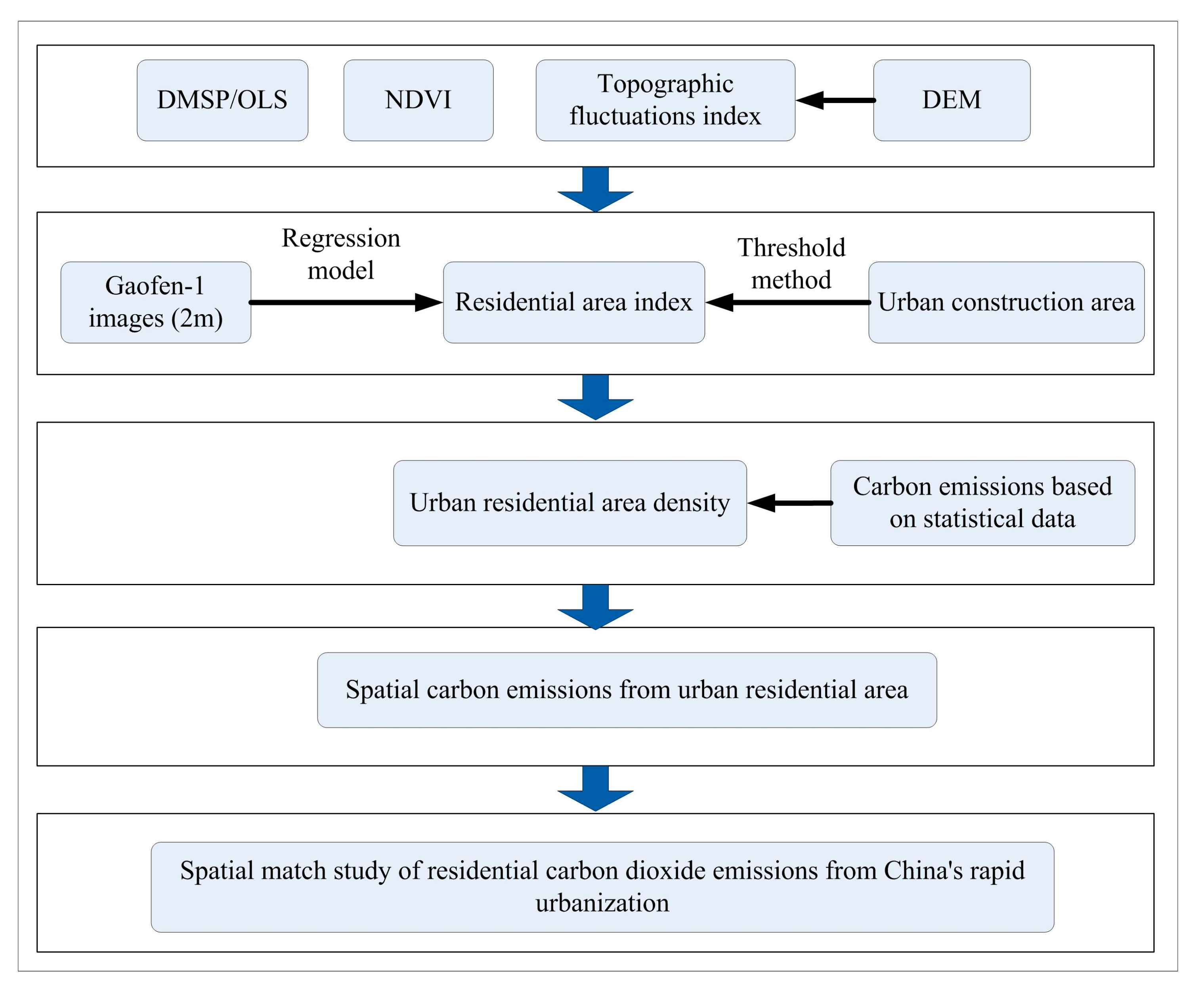
In this study, the geospatial data used for spatial simulations included DMSP/OLS, Normalized Difference Vegetation Index (NDVI), digital elevation model (DEM), high-resolution images acquired by the Gaofen-1 Imaging Satellite, and the 1 km grid Gross domestic product (GDP) dataset of China. The source of the DMSP/OLS data was from United States’ National Centers for Environmental Information (
http://ngdc.noaa.gov/); the NDVI and DEM data was from the Geospatial Data Cloud platform (
http://www.gscloud.cn); the Gaofen-1 images were obtained from the Satellite Surveying and Mapping Application Center under the National Administration of Surveying, Mapping and Geoinformation (
http://www.sasmac.cn); and the 1 km grid GDP dataset was from the Global Change Research Data Publishing and Repository (
http://geodoi.ac.cn/). The statistical data used is from the Urban Statistical Yearbook of China, Urban Construction Statistical Yearbook of China, Statistical Yearbook of Henan Province, and Statistical Yearbook of Zhengzhou City. A visual representation of the study’s methodology is shown in
Figure 2.
3.1. Urban Residential Area
DMSP/OLS data are generally useful for extracting information of urban residents’ activities. However, these contain flaws such as pixel saturation or overflow. MODIS provides time series multi-spectral remote sensing images and is used to calculate the NDVI. Since the NDVI is positively correlated with vegetation density and negatively correlated with residential area, this characteristic can be used to extract information about urban land cover [
45,
46]. The terrain of a region can be described using the macroscopic relief degree of land surface (RDLS). Overall, population densities and urban residential areas generally decline with increasing RLDS [
47,
48,
49,
50]. Another way to describe terrain is with terrain fluctuation index (TFI), proposed by Xiong et al. [
51], which simultaneously considers the three factors of elevation, slope, and aspect to comprehensively describe spatial fluctuations.
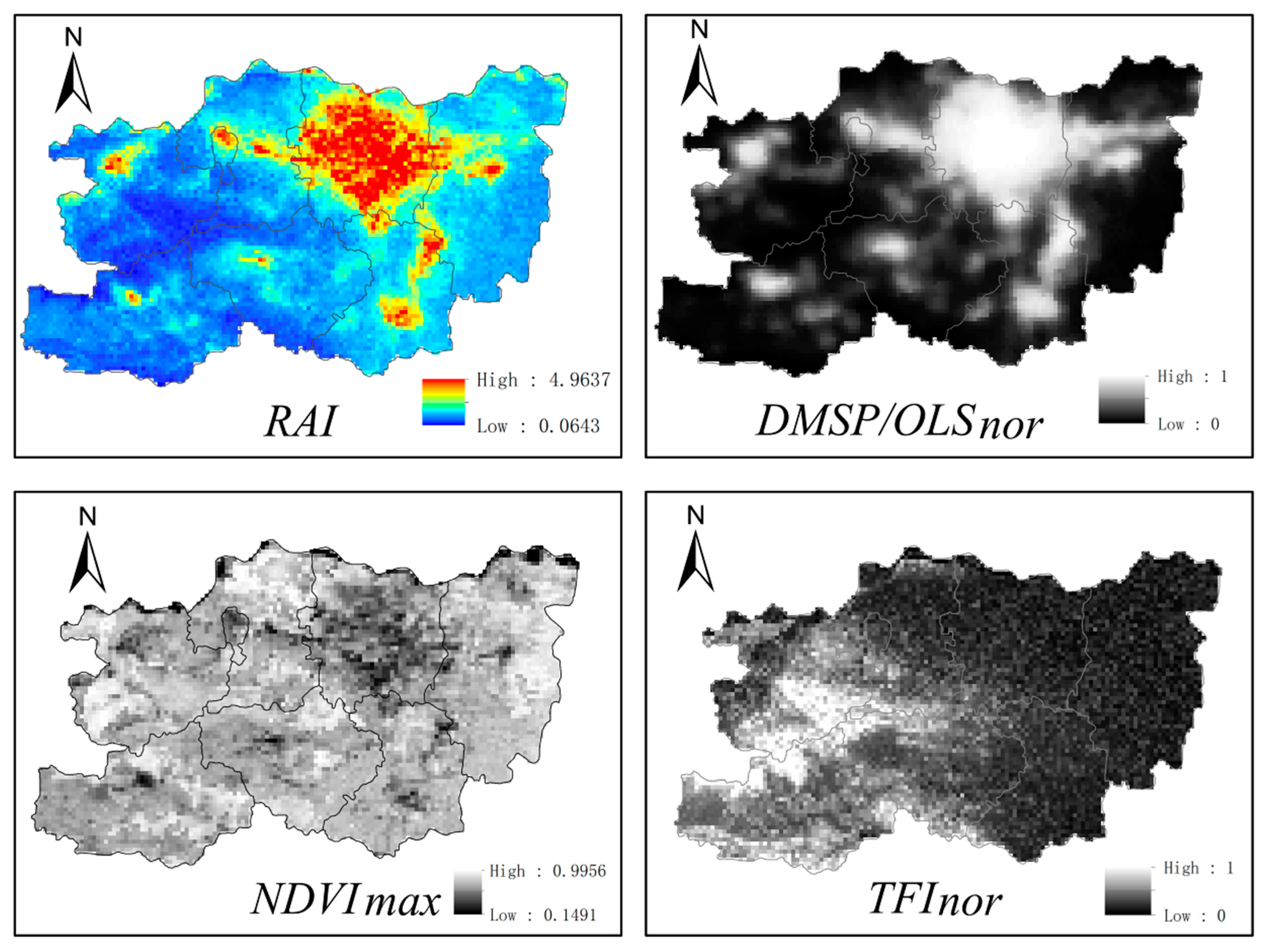
Since DMSP/OLS, NDVI, and TFI are all correlated with urban residential area, but have their respective flaws [
52], these factors were reintegrated to build the residential area index (RAI) using Equation (1).
where
OLSnor is normalized night-time lights;
NDVImax is maximum NDVI within one year; and
TFInor is normalized TFI.
The equations for calculating OLSnor, NDVImax and TFInor are stated below.
i Normalization of night-time lights
The normalization process converts DMSP/OLS values to 0–1 and is done using Equation (2).
where OLS indicates a particular pixel value in the images of night-time lights, and
OLSmin and
OLSmax represent the minimum and maximum values in those images for the entire research area, respectively.
ii NDVI
The NDVI is obtained by combining the spectral reflectance characteristic of green vegetation with the reflectivity of the near-infrared, infrared, and other bands. The NDVI must be processed because green vegetation undergoes specific seasonal cycles. This is usually done by extracting the maximum NDVI value within a year as shown in Equation (3).
where
NDVI1,
NDVI2, …,
NDVIn refer to the individual frames of NDVI images within one year.
iii Calculation of the TFI
The method for calculating TFI is shown in Equation (4) [
51].
where TFI is the topographic fluctuation index;
E and
are the elevation value of any random point in space and its average elevation value within the region where it is located, respectively;
S and
are the slope value of any random point in space and its average slope value within the region where it is located, respectively; and Δ
A is calculated using Equation (5), in which the differences in aspect between any random point in space and its adjacent eight points are summed, averaged, and then divided by 180°.
where
A is the aspect value of any random point in space,
Ai is the aspect value of a particular point adjacent to
A, and
i is 1, 2, 3, ..., 8.
The range of pixel values for the TFI is 0.13–2.00. Larger values indicate steeper topography, which makes the location less conducive for human habitation. The normalized equation for TFI is shown in Equation (6).
where
TFImin and
TFImax are the minimum and maximum TFI values within the region, respectively.
RAI gives mixed pixel results for urban residential area, so the following procedure is used to decompose these mixed pixels. First, residential area densities (RAD) are obtained through visual interpretations of high-resolution remote sensing images from Gaofen-1. The correlation between RAD and the RAI is used to build a regression model. Inversion of the regression model gives RAD for the entire research area. Using statistical data of the built urban area, the threshold method is applied to extract the spatial pattern of the urban residential area [
53]. The process of applying the threshold method is: (i) pixels are arranged in descending order by RAI; (ii) the corresponding residential areas are cumulatively added to gradually approximate the value of the urban construction area in the district; (iii) this process is continued until the difference between the cumulative value and the value of the urban construction area reaches the minimum value. Finally, that value is treated as the threshold and is used for extracting the spatial pattern of urban residential area.
3.2. Spatial Carbon Emissions
In this study, urban residential carbon emissions (RCE) refer to the emissions produced by residential usage of coal gas, natural gas, liquefied petroleum gas (LPG), household electricity, and central heating. This is calculated using Equation (7).
where
CT represents total carbon emissions from the urban residential area;
CF represents RCE produced by usage of coal gas, natural gas, and LPG for daily living;
CE represents RCE produced by usage of household electricity; and
CH represents RCE produced by central heating. The unit of measurement is tonne CO
2 (tCO
2).
The specific methods are stated below.
i Calculating emissions from usage of coal gas, natural gas, and LPG
This is based on energy consumption and the coefficients for calorific value and carbon emissions, and calculated using Equation (8).
where
k refers to the three types of residential energy consumption;
Ek is the consumption of energy type
k (unit: 10
4 m
3 for coal gas and natural gas, and t for LPG);
NCVk is the average low calorific value of energy type
k (unit: MJ/m³ for coal gas and natural gas, and MJ/kg for LPG); and
Ak is the carbon emission coefficient of energy type
k (unit: kgCO
2/MJ).
ii Calculating emissions from usage of household electricity
Emissions from electricity usage can be calculated directly through multiplication of electricity consumption and its carbon emission coefficient, as shown in Equation (9).
where
Ee is the household electricity consumption (unit: MWh) and
Ae is the carbon emission coefficient of electricity (unit: tCO
2/MWh).
iii Calculating emissions from central heating
The energy consumed by central heating is converted to equivalent standard coal, the carbon emission coefficient of which is then is used to determine final emissions. The calculation is shown in Equation (10).
where
Eh is the residential area for central heating (unit: 10
4 m
2);
Qc is the coal consumption index per unit residential area for central heating (unit: kg/m
2); and Ah is the carbon emission coefficient for standard coal (unit: kgCO
2/kg).
The values used in this study for the parameters described above are summarized in
Table 1.
The carbon emissions from an urban residential area can be calculated using Equation (11).
where
Cij is the carbon emissions in Pixel
i of District
j (unit: tCO
2);
Kj is the amount of CO
2 emitted by urban residents in District
j; and
RADij is the urban residential area density for Pixel
i of District
j.
Equation (12) can be used for obtaining
Kj:
where
CTj is the total emissions of District
j, calculated using Equation (1) (unit: tCO
2), and Ʃ
RADij is the sum of all urban residential area densities within District
j.
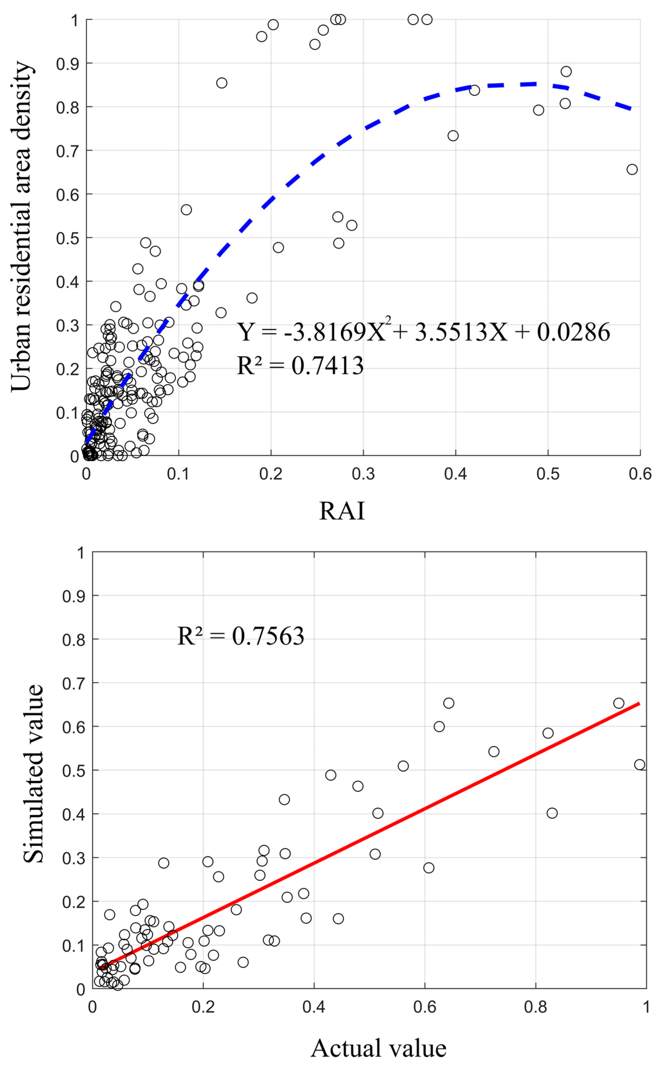
The correlation between urban residential area densities and RAI was used to establish a regression model. Using visual interpretation, 400 samples of urban residential area densities were obtained from the Gaofen-1 high-resolution (2 m) remote sensing images. 70% of the samples were selected for building quadratic polynomial model. This model was verified via 2 steps. First, the remaining 30% of the samples were used for accuracy testing based on the model, and second, remote sensing software (ERDAS IMAGINE 9.2) was used to test the Kappa coefficient.
3.3. Identifying Spatial Patterns Using SDE
In spatial mismatch study, standard deviational ellipse (SDE) spatial analysis technique is usually used to reveal the overall spatial distribution characteristics of geographical elements and the spatiotemporal processes of their evolution [
54,
55,
56]. Deden Rukmana [
57] utilizes SDE as a measure of dispersion of the prior addresses of the homeless around the mean center in two dimensions. It is found that the prior addresses of homeless categories are less tied to neighborhoods of high poverty than those of homeless men and homeless men-dominated categories. The SDE map produced by Sabine Dörry and Olivier Walther [
58] shows that large spatio-cultural differences are still prevailing among network actors, thus potentially impacting decisions taken in policy networks.
It uses the average center for the spatial distribution of geographical elements to define the center of the ellipse, and the standard deviations of those elements along the x- and y-axis to define the long and short axes of the ellipse, respectively. By comparing the long and short axes, one can determine whether the distribution of elements has been stretched. The long axis is defined as the main direction in which the elements are distributed and is indicated using the azimuth. Those covered by the SDE characterize the main body region in which the elements are spatially distributed. Its distribution area reflects the density in the distribution of the elements.
Standard deviation along the
x-axis:
Standard deviation along the
y-axis:
where (
xi,
yi) represents the coordinates;
wi is the value of the factor;
(, ) is the weighted average center;
θ is the elliptical azimuth, which represents the angle formed by the long axis of the ellipse as it rotates from true north in a clockwise direction;
and
are the deviations in coordinate between its location and the average center, respectively; and σ
x and σ
y are the standard deviations along the
x- and
y-axis, respectively.
To analyze spatial match, the SDE technique was applied to both carbon emissions and to GDP. The data used for GDP was a 1 km grid GDP dataset prepared by the Chinese Academy of Sciences (
http://www.geodoi.ac.cn/webcn/doi.aspx?Id=125) after comprehensive analysis of land use patterns arising from human activities and the laws of spatial interactions between those patterns and GDP. This information was used to construct a spatial correlation model between land use types and GDP amounts for the primary, secondary, and tertiary industries. Next, the location theory and spatial statistics were used to comprehensively analyze the spatial characteristics and regional differences in the socioeconomic development of China. The results are expressed quantitatively and partitioned hierarchically. A certain number of representative counties were selected from each sub-zone to act as the sample counties for modeling. The various data items of the sample counties were then used as the bases to establish the GDP spatial distribution model. This model was used to spatialize the GDP statistical data by county, thereby generating the 1 km grid dataset for GDP spatial distribution. Accuracy testing of the spatial GDP data indicated that the relative errors were 6%. Thus, the 1 km grid dataset was used as the standard GDP data for this study.
4. Results and Discussion
4.1. Urban Residential Carbon Emissions
The amount of urban residential emissions by Zhengzhou in 2010 (
Table 2) reached 7921.93 ktCO
2, with the metropolis district having contributed 5309.77 ktCO
2 (67.03%). The largest contributors outside the metropolis district were Gongyi District (8.12%), followed by Xinmi District (7.92%). Xingyang District is the smallest contributor, accounting for only 2.85% of the total emissions. The various districts, arranged in descending order by total emissions, are as follows: the metropolis district > Gongyi District > Xinmi District > Xinzheng District > Zhongmu District > Dengfeng District > Xingyang District.
4.2. Spatial Carbon Emissions from Urban Residential Area
Figure 3 shows the RAI, DMSPM/OLS, NDVI, and TFI of Zhengzhou in 2010. The latter three indices were used to calculate the RAI, which is shown in the upper left quadrant.
In
Figure 4, a quadratic polynomial model best fits the data, resulting in coefficients of determination values (R2) of 0.741 and the F-value was 268.688 (
p < 0.0001). Such a model indicates that urban residential area density increased as RAI increased. The bounded functional form characteristic from the negative quadratic polynomial model will make urban residential area density attain a finite value and remain at that level without exceeding it as the value of the RAI continues to increase. The result of evaluation is similar to actual circumstance: we found a high linear correlation coefficient (0.756) between the actual and simulated values for residential area densities (
p < 0.01). The Kappa coefficient of the model was found to be 0.72. As a result we believe that the accuracy of this model is acceptable and the results are reliable.
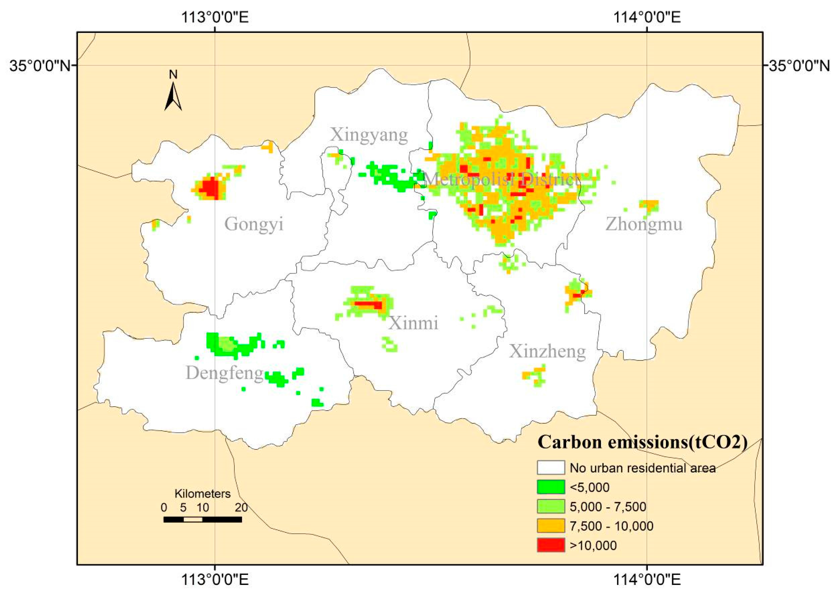
Based on Equations (11) and (12), the spatial pattern of carbon emissions from urban residential areas in the rapidly urbanizing Zhengzhou in 2010 was calculated and is shown in
Figure 5. The emissions in the Zhengzhou metropolis district were high, with the amounts from Jinshui, Guancheng Hui, Erqi, Zhongyuan, and Huiji being higher than that of Shangjie. This is because Shangjie is an administrative enclave and segregated from Zhengzhou metropolis’s main metropolitan area. Xingyang District is located between Shangjie and the Zhengzhou metropolis district. It serves as the link between the two, resulting in the contiguous spatial pattern that covers the metropolitan area—Xingyang District-Shangjie Sub-district.
The ranking in terms of average emission densities for each district was different: instead of the metropolis District, Gongyi District took the top position. At 8.91 ktCO2/km2, its average emission was 2.5 times that of the lowest-ranking Dengfeng District and 2.45 times that of Xingyang District. The metropolis District ranked second with an average emission density of 7.96 ktCO2/km2. The ranking of the various districts in terms of average emission per unit area are as follows: Gongyi District > the metropolis District > Xinzheng District > Zhongmu District > Xinmi District > Xingyang District > Dengfeng District. Gongyi District also had the highest emissions per square kilometer. At 13.95 ktCO2, it was 1.9 times that for the average of research area (7.23 ktCO2). The lowest was by Dengfeng District: at 2.49 ktCO2, it was only 0.34 times that of the average of research area.
The ZNA, located in the eastern section of Jinshui sub-district, is urbanizing rapidly. This has caused higher emissions from northeast Zhengzhou. The distribution is contiguous and encroaches into Zhongmu District. The Zhengzhou Airport Economic Zone (ZAEZ), with the Xinzheng International Airport as its focal point, has undergone accelerated urbanization in recent years. The emissions from this zone are substantial and quite far-ranging, as can be seen in
Figure 5. Another location in which emissions started rising recently is Longhu Town, located in the northern section of Xinzheng District. For Xinzheng, Xinmi, Gongyi, and Dengfeng and Zhongmu Districts, the spatial pattern was one of higher amounts in the center, followed by a gradual decline towards the peripheries.
4.3. Spatial Patterns Identified with SDE
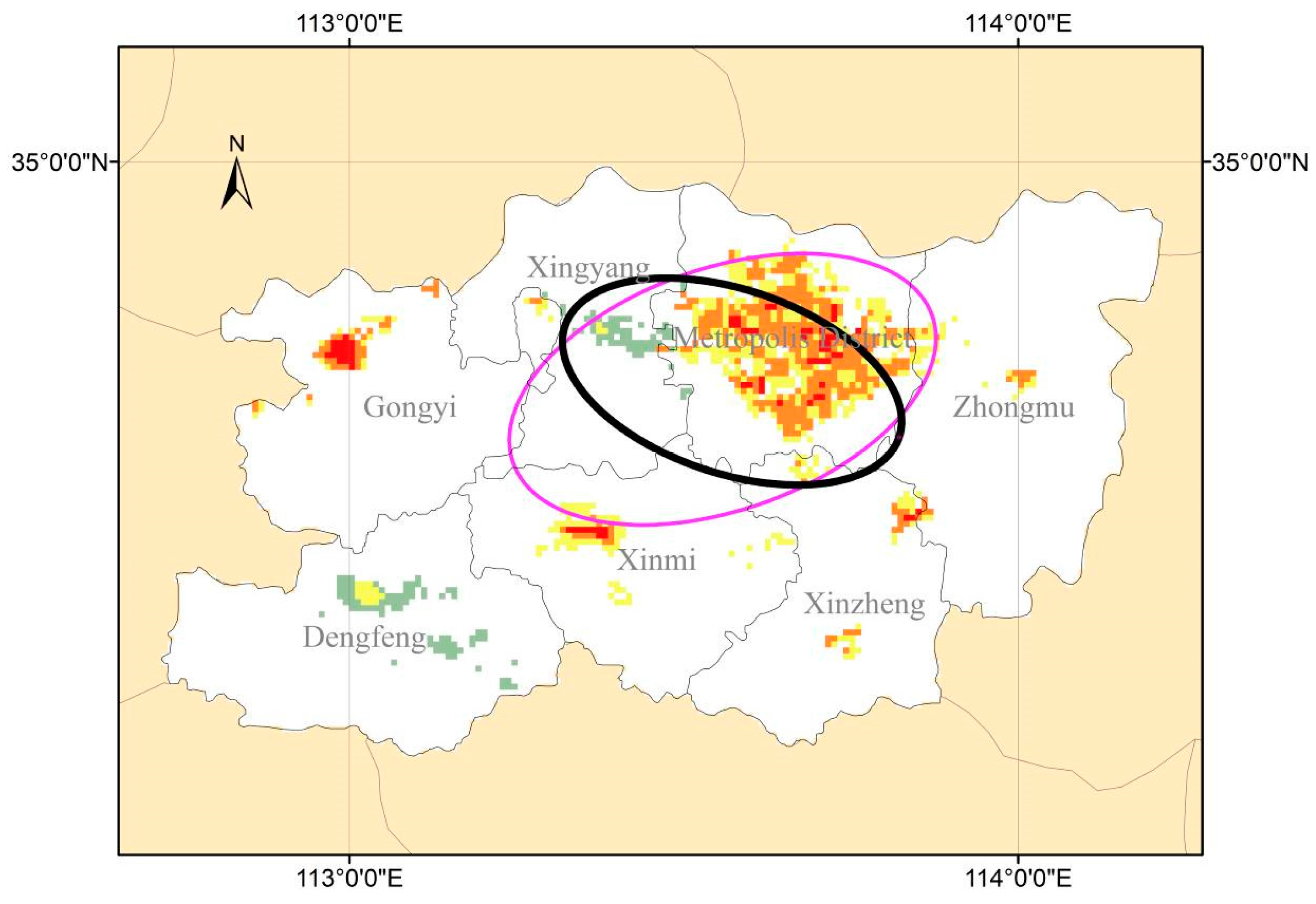
The SDE analyses of spatial patterns of emissions in 2010 based on (i) night-time lights and (ii) traditional statistical data are compared in
Figure 6. The former presented a spatial pattern in a northwest-southeast direction. This was caused by Gongyi District, located in northwest Zhengzhou. Its rapid urbanization in recent years resulted in it being placed first in terms of emission per unit area. Along that direction, Gongyi District is also in linear alignment with Xinmi and Xinzheng Districts, both of which are high emission density. Dengfeng District, which is located in southwest Zhengzhou and whose development is driven by tourism, is the opposite: not only did it have the smallest emission per unit area, its proportion of the amount was also small.
On the other hand, the SDE analysis of spatial patterns of emissions from traditional statistical data resulted in a pattern with northeast-southwest direction, which is almost the same direction as the shape of Zhengzhou. The SDE distribution area was also much larger. These deviations were caused by dependence on the statistical unit, which has a larger scale. We believe that the SDE analysis was greatly improved by the use of night-timelighting for spatial simulations: the northwest-southeast alignment of the ellipse presented the actual spatial pattern of emissions and the smaller SDE distribution area better reflects the aggregative tendency of emissions.
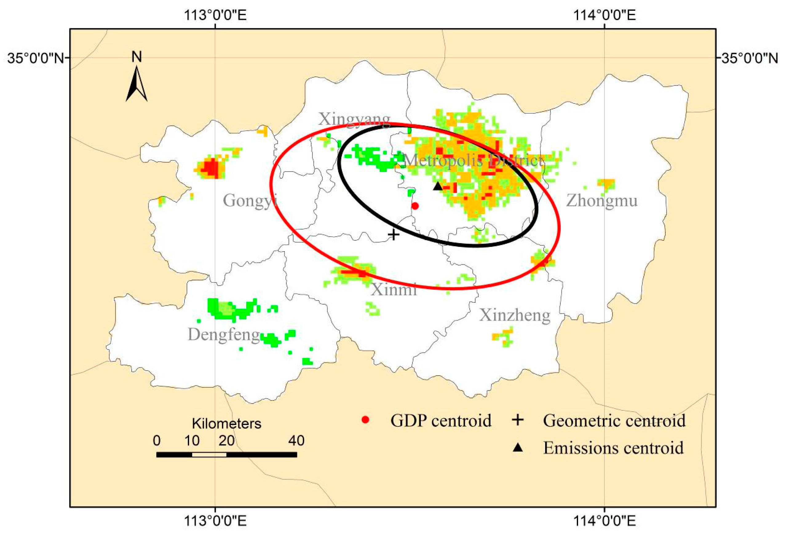
The comparison between the SDE analyses of spatial patterns of emissions and 1 km grid GDP dataset of China is shown in
Figure 7.
It can be seen from
Figure 7 that the emissions SDE centroid is biased towards the northeast and located within the metropolis district. It is 18.86 km away from the geometric centroid (marked with a “+”), located at the intersection between Xingyang and Xinmi District. This is because emissions were heterogeneous and spatially aggregated at the city districts located in northeast Zhengzhou. The SDE centroids for emissions and GDP do not overlap: the centroid for the latter is located at the intersection between Xingyang District and the metropolis District, with a 9.05 km distance between the two. Thus, there is mismatch in spatial pattern between emissions and GDP.
It can also be seen from
Figure 7 that the emissions SDE centroid deviated further from the regional geometric center than GDP SDE centroid, meaning that emissions are more heterogeneous than GDP. For emissions, the direction of the SDE long axis is 108°25′23″, which is in between the east-west and northwest–southeast directions. It is basically consistent with the line connecting Gongyi District and ZAEZ. It is also similar to the GDP SDE direction, whose long axis is in the direction of 102°06′06″. This indicates that even though the spatial pattern of emissions and GDP were not consistent, there was still a correlation between the two.
4.4. Spatial Patterns Evolution Identified with SDE
The spatial patterns of emissions from 2000 to 2012 were calculated and the results were compared with the 1 km grid GDP dataset for 2000, 2003, 2005 and 2010.
Figure 8 shows, for the SDE of emissions, the length of the long axis, ratio of the short axis to long axis, azimuth; and the centroids of SDE for emissions and GDP.
Between 2000 and 2012, the length of SDE long axis decreased from 31.21 km in 2000, to 29.34 km in 2003, 29.10 km in 2006, 28.34 km in 2009, and 28.01 km in 2012. The corresponding SDE area shrank from 1586 km2 in 2000, to 1477 km2 in 2003, 1429 km2 in 2006, 1426 km2 in 2009 and 1344 km2 in 2012. Such a reduction indicates that the growth rates of emissions within the SDE were relatively faster than those outside, causing the SDE coverage to contract. Although there were slight fluctuations in the ratio of the SDE short axis to its long axis between 2000 and 2012, the overall change was not substantial. This shows that for the various districts in Zhengzhou, their emissions growth rates were relatively balanced.
Generally, spatial patterns of emissions existed along the northeast-southwest direction; there was a slight azimuthal increase amid the fluctuations for 2000–2012. Specifically, there was a clockwise rotation of a small magnitude that increased from 104°08′18″ in 2000, to 105°5′13″ in 2003, 106°8′31″ in 2006, 106°55′52″ in 2009, and 110°56′31″ in 2012. This azimuthal increase indicates that the growth rate of emissions was faster in areas corresponding to the upper right portion of the SDE axis than those of the lower left portion. Relative to emissions, the magnitude of change was smaller for GDP with respect to the SDE long axis, ratio of the SDE short to long axes, and SDE azimuth.
The spatial simulation model based on night-time lights produced a detailed representation of evolution of the spatial pattern of emissions (
Figure 8). In 2000–2004, the SDE centroid was in Zhengzhou’s metropolis district. After Zhengzhou was designated the core CPMR city in 2006, the pace of urbanization accelerated rapidly. Urban development in the ZNA was especially remarkable. Being a new development area, ZNA’s urbanization became the main factor affecting the spatial migration trajectory of emissions, causing the SDE centroid to shift eastward.
From 2010, the ZAEZ’s urbanization increased quickly under governmental promotion and contributed significantly to Zhengzhou’s urbanization level. It was accompanied by expedited emissions increases, resulting in the significant shift of the SDE centroid northward. These complex changes—from northeastward, to northwestward, southeastward, northwestward, eastward, and finally northward—depicted the basic evolution in characteristics of emissions, which was basically consistent with the urban development and implementation strategies stated in the Urban Master Plan for Zhengzhou City (2008–2020): “to focus on the east (promote and improve the ZNA’s development) while taking into account the west; nurture the growth of the south but control that of the north.”
The spatial migration trajectories of both emissions and GDP were shifted towards the northeast. However, the SDE centroid for GDP was relatively more stable and its range of movement was smaller. The SDE centroid for emissions was much more active and deviated further away from the Zhengzhou’s geometric center. On the whole, the spatial pattern of emissions was more volatile and less stable than that of GDP during the rapid progress of urbanization. With the rise of new urbanization areas such as the ZNA and ZAEZ, the movement of emissions had become more prominent and accentuated.

 ,
, 


