Disentangling the Complex Effects of Socioeconomic, Climatic, and Urban Form Factors on Air Pollution: A Case Study of China


1
Center for Human-Environment System Sustainability (CHESS), State Key Laboratory of Earth Surface Processes and Resource Ecology (ESPRE), Faculty of Geographical Science, Beijing Normal University, Beijing 100875, China
2
Key Lab of Urban Environment and Health, Institute of Urban Environment, Chinese Academy of Sciences, Xiamen 361021, Fujian, China
3
School of Life Sciences and School of Sustainability, Arizona State University, Tempe, AZ 85287, USA
*
Authors to whom correspondence should be addressed.
Sustainability 2018, 10(3), 776; https://doi.org/10.3390/su10030776
Submission received: 30 December 2017
/
Revised: 10 February 2018
/
Accepted: 8 March 2018
/
Published: 12 March 2018
(This article belongs to the Special Issue Defining and Assessing Landscape and Urban Sustainability: Linking Spatial Patterns, Ecosystems Services, and Human Wellbeing)
Abstract
:China’s tremendous economic growth during the past three decades has resulted in worsening air quality in most of its cities. However, the spatiotemporal patterns and underlying drivers of air pollution in China remain poorly understood. To address this issue, we used stepwise regression to identify major socioeconomic, climatic, and urban form factors influencing air pollution in 69 major cities across China. Our results showed that social factors such as population size and density were positively correlated with emissions of PM2.5, PM10, NOx, and SO2. Economic factors such as Gross Domestic Product (GDP) and GDP of secondary industry were positively correlated with industry and transportation emissions but negatively correlated with residential emissions of air pollutants. Urban form attributes such as measures of urban fragmentation and contiguity were important in explaining patterns of emissions from residential, power generation, and transportation sectors. As for climatic factors, higher precipitation, higher wind speed, and higher temperatures were all negatively correlated with air pollution levels. We also found that the effects of socioeconomic, climatic, and urban from factors on air pollution levels varied considerably among seasons and between the annual and seasonal scales. Our findings have useful implications for urban planning and management for controlling air pollution in China and beyond.
1. Introduction
Over the past three decades, rapid urbanization in China has been unprecedented in terms of both speed and scale and more than half of its population now live in cities [1,2]. However, China’s tremendous economic achievements have resulted in a number of environmental problems, including the deterioration of air quality [3,4,5,6]. Increased air pollution may lead to the cardiopulmonary morbidity and mortality of people, especially the young and elderly [1,7,8].
High PM2.5 concentrations have occurred over a vast region of China since the end of the 20th century [9,10,11]. Increased SO2 emissions have mainly resulted from human activities, such as industrial emissions [12]. Emissions of nitrogen oxide (NOx) and carbon monoxide (CO), and concentrations of ozone (O3) increased dramatically due to the increased number of vehicles [13], and were accompanied by an increase in emissions of greenhouse gases (e.g., CO2) [14,15]. Recent studies have related these spatial patterns of air pollution to environmental and socioeconomic factors depending on distinguished mechanisms [6,16,17,18,19]. For example, wind not only dissipates air pollutants in the city, but also transports pollutants from industrial areas to urban areas [12,20]. Compact cities with mixed land uses were reported to have less transportation emissions than sprawl cities [17,21], but also could trap more air pollutants from urban construction, thereby leading to higher pollution concentrations [22]. Bechle et al. (2011) [6] found that air pollution levels first increased with rising income levels (GDP per capita), and then decreased when GDP per capita exceeded $30,000, an observation that seems consistent with the Environmental Kuznets’ Curve [23].
Overall, air pollution and its spatiotemporal patterns are influenced by a number of socioeconomic and environmental factors [6,16,21,22,24,25,26,27,28]. However, a comprehensive understanding of the underlying drivers of air pollution in China’s cities is still lacking from multiple perspectives (air pollutant emissions and concentrations) and time scales (year and season). Thus, the main objectives of this study were (1) to identify the major factors influencing urban air pollutant emissions, and (2) to understand how climatic, socioeconomic, and urban form factors may affect urban air pollution patterns in China.
2. Materials and Methods
2.1. Study Cities
High concentrations of PM2.5—much higher than the 10 µg/m3 standard set by World Health Organization (WHO) air quality guidelines—occurred over a vast region of China since 1999, ranging from southern Inner Mongolia to Guangdong latitudinally, and from the east coast to central Sichuan longitudinally, plus the southern part of Xinjiang Province [9,11]. In this study, we selected 69 cities across this region based on data availability (Figure 1).
2.2. Potential Socioeconomic, Climatic, and Urban Form Factors
Previous studies have shown that urbanization, industrialization, and economic development can all contribute to air pollution [3,12,13,16,18,29,30]. Sand-dust storms in spring [4], secondary aerosol generation O3, and PM2.5 pollution in summer [31], agriculture biomass burning in autumn [32], and coal burning for winter heating [20] are the main drivers for seasonal air pollution events, whereas climatic conditions, such as high humidity and low wind speed, are key environmental factors [33]. Thus, we collected air pollution data, socioeconomic data, climatic data, and land use/cover data for the 69 cities in China based on data availability (Figure 1).
2.2.1. Air Pollution Measures
Air Pollution Index (API) and PM2.5, PM10, NOx, and SO2 emissions from industry, power generation, residential sector, and transportation were used to represent air pollution levels (Table 1). Daily API data for 69 cities in 2010 were downloaded from the Chinese Ministry of Environmental Protection website (MEP) (http://www.zhb.gov.cn/). The API level is based on the levels of three atmospheric pollutants, including SO2, NO2, and PM10 measured by monitoring stations for each city.
Anthropogenic emissions of air pollutants for each city in 2010 were extracted from the database created by [34] which was generated according to the Multi-resolution Emission Inventory for China (MEIC) (Table 1). The MEIC is a bottom-up emission inventory framework developed and maintained by Tsinghua University, China, using a technology-based methodology to calculate air pollutant emissions [34]. The database included emissions from more than 700 anthropogenic sources that were aggregated into four categories: power generation, industry, residential sector, and transportation [34]. For example, the emissions from combustion of coal, oil, gas, biomass, and waste (e.g., municipal and industrial waste) for power generation were classified into power generation category. The industry category included the emissions from combustion of coal, oil, gas, waste, and biomass and non-combustion processes (e.g., brick production and iron sintering). The vehicle emissions from combustion of oil and gas were classified into transportation category. The emissions from combustion of coal and biomass for heating and combustion of gas for cooking were classified into residential sector.
2.2.2. Climatic Factors
Data on daily temperature (°C), precipitation (mm), wind speed (m/s), relative humidity (%), and sunshine duration (h) were obtained from the China Meteorological Data Sharing Service System (http://cdc.nmic.cn) (Table 1). Annual and seasonal averaged values of each climatic factor were calculated from daily data and selected as potentially climatic factors.
2.2.3. Socioeconomic Factors
Data on Gross Domestic Product (GDP in Chinese Yuan, CNY), GDP of secondary industry (CNY), and population size (permanent residents) in 2010 were derived from the Statistical Yearbook of the National Bureau of Statistics (http://www.stats.gov.cn/) as potential socioeconomic factors. For each city, we divided the overall GDP and GDP of secondary industry by population to calculate per capita GDP and per capita GDP of secondary industry. Population for each city was divided by its total area within administrative boundary to calculate population density (Table 1).
2.2.4. Urban Form Metrics
Ten class-level landscape metrics were used to represent urban form in this study: Total built-up Area (TA), Patch Density (PD), Mean Patch Area (MPA), Percentage of Landscape (PLAND), Largest Patch Index (LPI), Area Weighted Mean Fractal Dimension (AWMFD), Edge Density (ED), Landscape Shape Index (LSI), Clumpiness index (CLUMPY), and Aggregation Index (AI), all of which were computed for the urban patch type (see Appendix A for detailed acronyms and descriptions of these metrics). TA and PLAND are area-related composition indicators that represent total built-up area and its proportion, respectively. PD, MPA, and LPI are different measures of the degrees of fragmentation of built-up areas. ED indicates boundary abundance of built-up area patches. LSI and AWMFD are measures of the shape complexity of built-up areas. CLUMPY and AI measure the degrees of clumping and the aggregation of built-up areas. The main justification for choosing these 10 metrics is that they have been widely used to characterize the spatial extent, fragmentation, shape complexity, and connectivity of urban landscapes [41,42,43,44,45,46,47], and have been related to urban air pollution in previous studies [6,16,17,21,22,24,26,48].
All these urban class-level metrics were computed using FRAGSTATS v4.2 [49], based on land use/cover data in 2010 with a spatial resolution of 1 × 1 km. The land use/cover data were obtained from the National Science & Technology Infrastructure of China, National Earth System Science Data Sharing Infrastructure (http://www.geodata.cn). The original dataset had six land cover types (forest, cropland, grassland, barren land, water body, and built-up area), and for the purpose of our analysis they were classified into two classes: built-up area and non-built-up area. The built-up area is a geographic region dominated by non-vegetated, human-constructed elements (proportion of built-up area higher than other five land use/cover types), such as settlements, buildings, roads, runways, and industrial facilities [2]. The non-built-up area included another five land use/cover types. The extent of each city was delineated as the total area within administrative boundaries of a prefecture-level city.
2.3. Quantifying the Relationships of Air Pollution with Socioeconomic, Climatic, and Urban Form Metrics
We used two sets of stepwise regression models (21 in total) to address the two research objectives. The first set of stepwise regression models (a total of 16) was used to identify the main factors associated with the emissions of air pollutants. In these models, the independent variables included six socioeconomic factors and 10 urban form factors, and the dependent variables were emissions of PM2.5, PM10, NOx, and SO2 from industry, power generation, residential sector, and transportation, respectively. Climatic factors were not included as the independent variables because they did not contribute to air pollutant emissions directly. The second set of stepwise regression models (a total of 5) was used to examine which factors were important to explaining the variations of air pollution levels on multiple time scales. In these models, the independent variables included five climatic factors, six socioeconomic factors, and 10 urban form factors, and the dependent variables were annual and seasonal API in spring, summer, autumn, and winter, respectively. The results of regression include correlation coefficient (R), adjust coefficient of determination (Adj. R2), F-test value (F-value), and probability value (p-value). Correlation coefficient is a measure of the strength between dependent and independent variables. Adjust coefficient of determination equals the proportion of the variance in the dependent variable that is predictable from the independent variables and gives some information about the goodness of fit of a model. F-value is the ratio of explained and unexplained variance and is used to compare regression models that have been fitted to data. Probability value is the probability of the statistical summary of a given model would be the same as the actual observed results and usually provides a significance level of the test. All these analyses were performed with SPSS v18.0 (IBM, Armonk, NY, USA).
3. Results
3.1. Spatial Patterns of Air Pollution in Chinese Cities
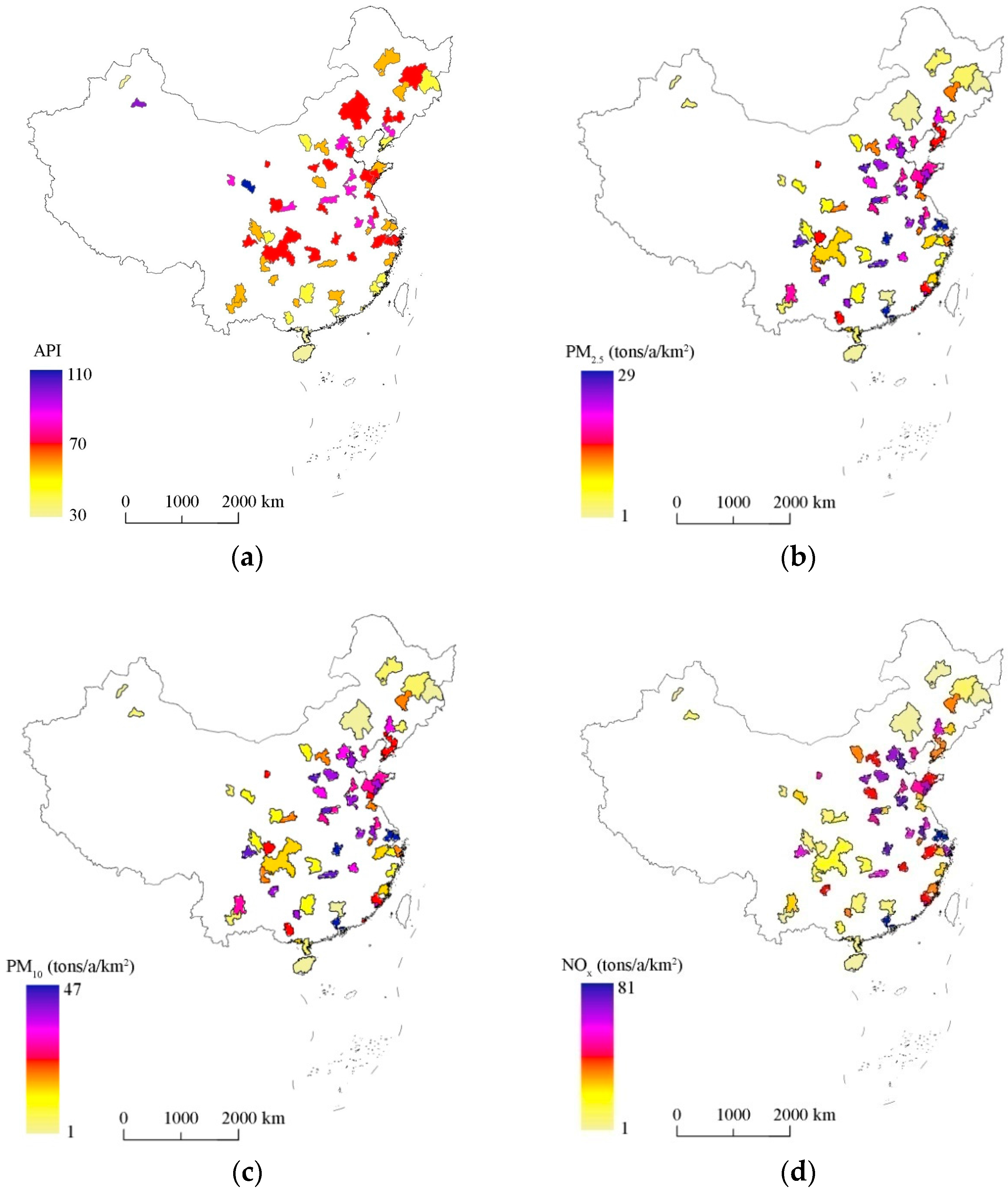
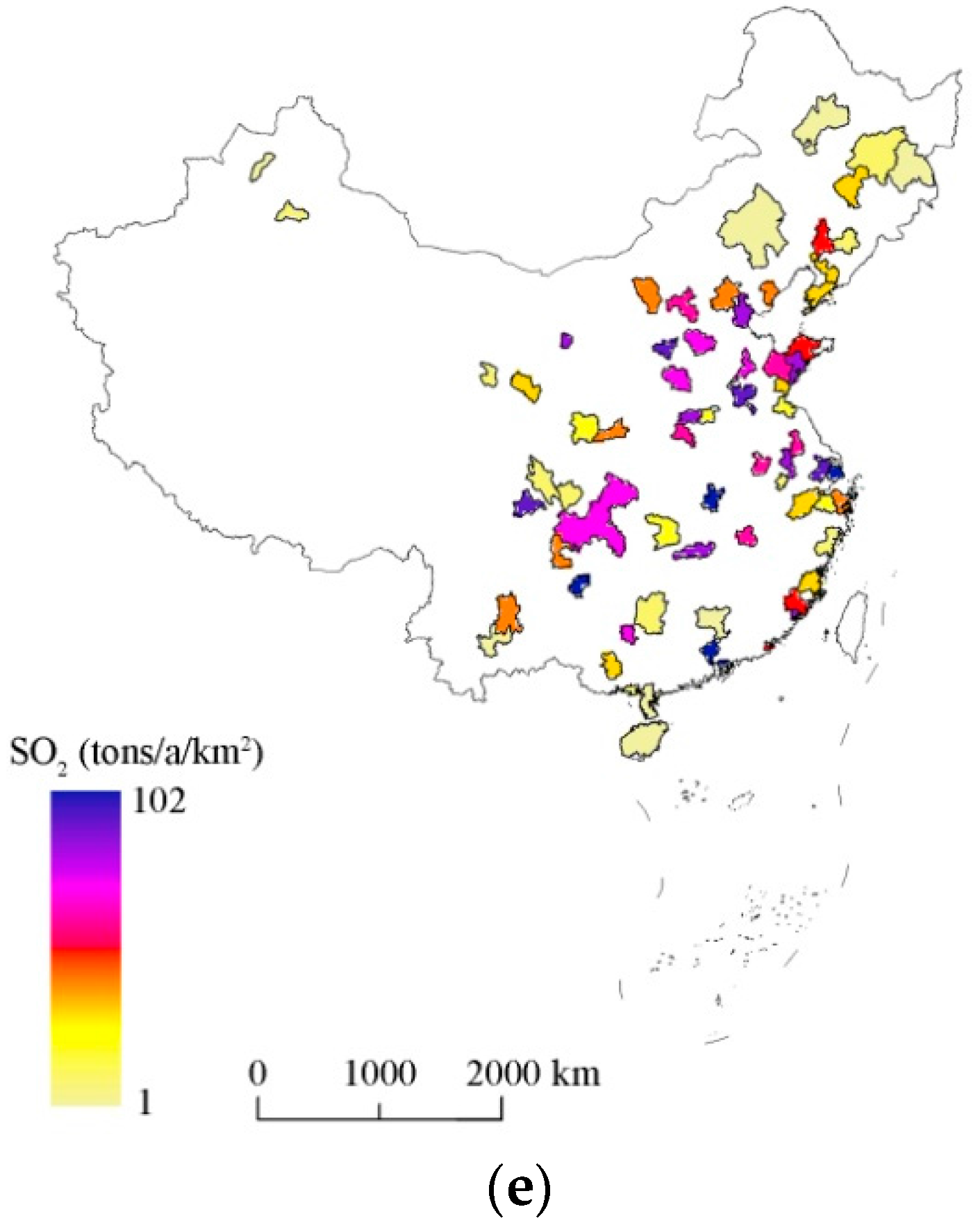
High values of API occurred in most of the 69 cities of China, especially those in the Northeast, the Beijing-Tianjin-Hebei region, and central Sichuan, plus Urumqi in Xinjiang Province (Figure 2a). High emissions of PM2.5, PM10, NOx, and SO2 occurred in cities located in the North China Plain (Beijing, Tianjin, Hebei, Shandong, Henan, northern Jiangsu, and northern Anhui) and the middle and lower reaches of the Yangtze River Basin (Figure 2b–e). Moreover, a large amount of SO2 was emitted from those cities located in the Sichuan Basin (Figure 2e).
3.2. Effects of Socioeconomic Factors and Urban Form on Emissions of Air Pollutants
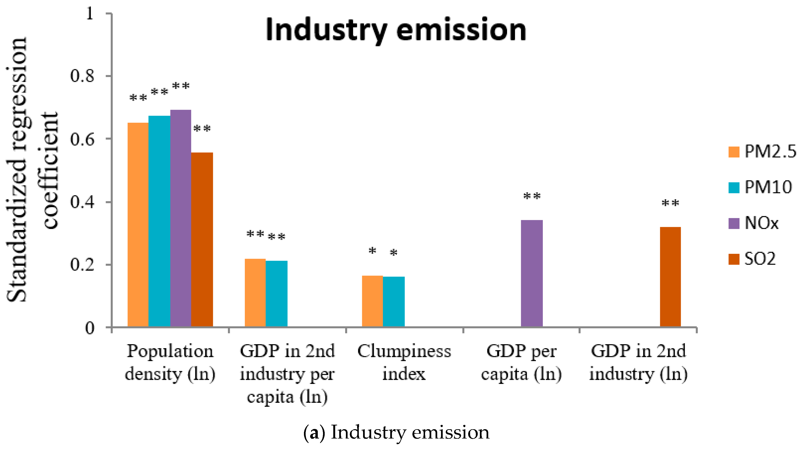
3.2.1. Industrial Emissions
In general, air pollutant emissions from industry were positively correlated with socioeconomic factors and urban form metrics. The regression models performed well in predicting industry emissions of PM2.5, PM10, NOx, and SO2, with adjusted R2 values of 0.685, 0.707, 0.771, and 0.631, respectively (Table 2). More specifically, these regression models identified population density, per capita GDP of secondary industry, and clumpiness as the best predictor variables for PM2.5 and PM10 emissions; population density and per capita GDP as the best predictor variables for NOx emissions; and population density and GDP of secondary industry as the best predictor variables for SO2 emissions (Figure 3a). All the above selected factors were significantly and positively correlated with the industry emissions of air pollutants (Figure 3a).
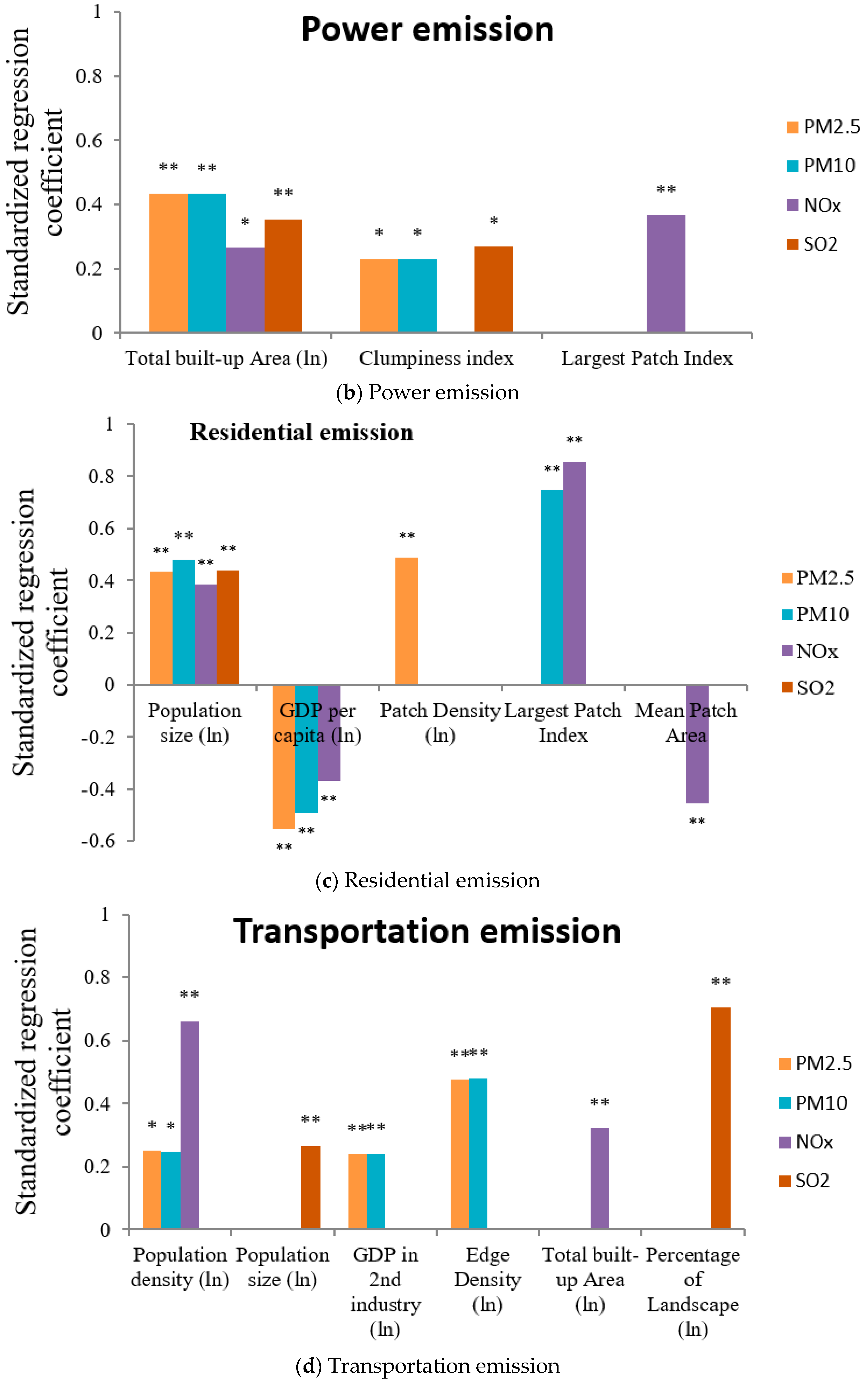
3.2.2. Emissions from Power Generation
Urban size and form had significant effects on air pollutant emissions from power generation. The values of adjusted R2 of the regression models for power-generation emissions of PM2.5, PM10, NOx, and SO2 were 0.277, 0.275, 0.307, and 0.227, respectively (Table 2). Total built-up area and clumpiness index were the best predictor variables for emissions of PM2.5, PM10, and SO2 (Figure 3b). Total built-up area and largest patch index of built-up area were the best predictor variables for NOx emissions (Figure 3b). A significantly positive relationship was observed between the power-generation emissions of air pollutants and the selected factors (Figure 3b).
3.2.3. Residential Emissions
In general, residential air pollutant emissions were positively correlated with urban size and form metrics, but negatively with economic factors. The values of adjusted R2 of the regression models for residential emissions were 0.441, 0.432, 0.64, and 0.181 for PM2.5, PM10, NOx, and SO2, respectively (Table 2). More specifically, residential emissions of PM2.5 were positively correlated with population size and patch density, but negatively with per capita GDP. Residential emissions of NOx were positively correlated with population size and largest patch index of built-up area, but negatively with per capita GDP. Residential emissions of PM10 were positively correlated with population size and largest patch index of built-up area, but negatively correlated with per capita GDP (Figure 3c). Only population size was significantly correlated with residential SO2 emissions, and a positive relationship was observed between them (Figure 3c).
3.2.4. Transportation Emissions
Air pollutant emissions from transportation were positively correlated with socioeconomic factors and urban form metrics. The regression models performed well in predicting transportation emissions of PM2.5, PM10, NOx, and SO2, with adjusted R2 values of 0.755, 0.754, 0.757, and 0.744, respectively (Table 2). More specific, major determinants of transportation emissions of PM2.5 and PM10 selected by regression models were population density, GDP of secondary industry, and edge density (Figure 3d). Population density and total built-up area were the best predictors for transportation emissions of NOx (Figure 3d). Population size and percent built-up area were the two predictors for transportation emissions of SO2 (Figure 3d). All the above selected factors were significantly and positively correlated with the transportation emissions of air pollutants (Figure 3d).
3.3. Effects of Climatic, Socioeconomic, and Urban Form Factors on API
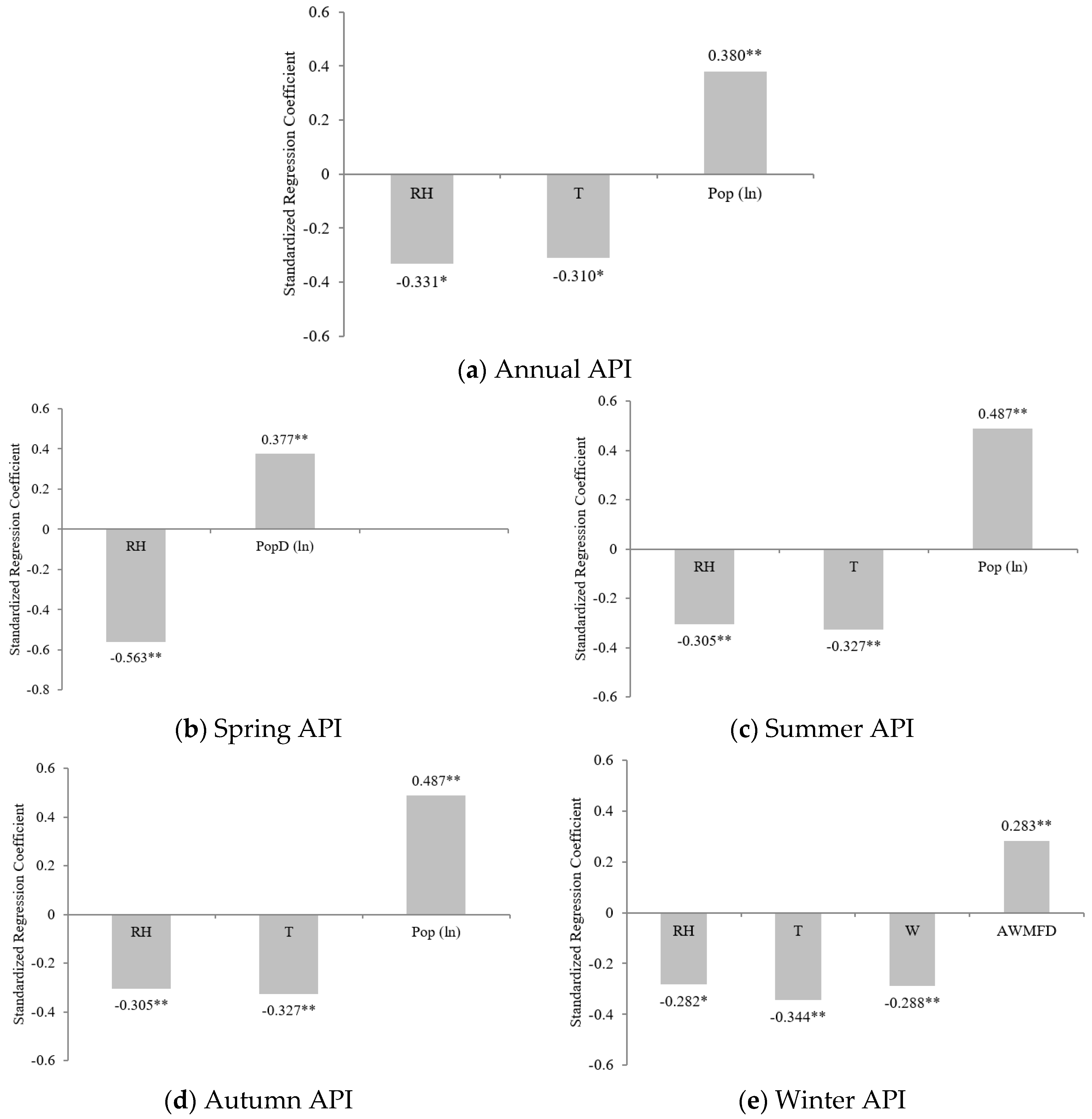
In general, API levels were positively correlated with socioeconomic factors (e.g., population size and density) and urban form metric (e.g., AWMFD), but negatively with climatic factors (e.g., humidity, precipitation, temperature, and wind). More specifically, the adjusted R2 value of regression models for annual API was 0.408 (p-value < 0.001) (Table 3). The annual API was positively correlated with population size but negatively with relative humidity and temperature (Figure 4a). The values of adjusted R2 of regression models for seasonal API were 0.309 (p-value < 0.001) in spring, 0.269 (p-value < 0.001) in summer, 0.124 (p-value = 0.005) in autumn, and 0.359 (p-value < 0.001) in winter (Table 3). Spring API was positively correlated with population density but negatively with relative humidity (Figure 4b); summer API was positively correlated with population size but negatively with relative humidity and temperature (Figure 4c); autumn API was positively correlated with population size but negatively with precipitation (Figure 4d); and winter API was positively correlated with AWMFD but negatively with humidity, temperature, and wind speed (Figure 4e).
4. Discussion
4.1. Which Socioeconomic and Urban Form Factors Were Related to Pollutant Emissions?
Our results indicated that socioeconomic variables were the dominant factors in predicting industry and residential emissions of air pollutants, with population density being the most important factor for industry emissions (Figure 3). Population density as a social factor was consistently and positively correlated with all kinds of emissions, followed by economic factors including GDP of secondary industry or per capita GDP of secondary industry. This phenomenon was probably due to the fact that industry dominated the economy in densely populated Chinese cities, which generally emitted a large amount of air pollutants. Larger urban population size and higher density tended to generate more residential and transportation emissions, and thus had higher contributions in Figure 3c,d. We also found that high-income cities (per capita GDP) experienced lower residential emissions. This might result from tighter environmental regulations and more public expenditures for lowering air pollutants emissions in high-income cities [22]. Moreover, sprawling cities, with higher patch density, lower mean patch size, and smaller largest patch index of built-up area, tended to generate more emissions of air pollutants due to its lower energy use efficiency than compact cities. A recent study has reported that the central heating systems in Chinese cities may reduce the urban household energy consumptions and PM2.5 emissions [50].
In contrast with the main factors for industrial and residential emissions, the composition and configuration attributes of the urban landscape were more important for explaining power and transportation emissions. Large cities, which had more extensive total built-up areas and more contiguous built-up areas (indicated by higher values of clumpiness index and largest patch index) tended to have greater power demands. However, parts of these power demands were fulfilled by those power plants located in other cities or even provinces, and needed a long distance power transportation. This discrepancy between local usage and emissions at other places may be the reason why the values of regression coefficients in the power generation sector were relatively lower than those values in industrial, residential, and transportation sectors (local emissions dominated). Moreover, fragmented cities with highly convoluted, irregular boundaries (higher edge density) were expected to have higher non-point emissions (primarily from automotives) [16], as well as higher secondary aerosol contributions (e.g., NO2 and SO2) to PM pollution [31]. In addition, higher GDP of secondary industry and population size (or population density) tend to have higher demands for transporting goods and commuting services, often leading to higher local air pollutant emissions.
4.2. How Did Effects of Climatic, Socioeconomic, and Urban Form Factors on Air Pollution Change with Season?
Our results show that all the three kinds of factors (climatic, socioeconomic, and urban form factors) may potentially affect API levels. Specifically, API levels were positively correlated with socioeconomic and urban form factors, but negatively with climatic factors. More precipitation helped decrease API levels due to the wet deposition effect [39]. In winter, relatively low horizontal wind speeds and higher urban shape complexity (fractal dimension) may hinder the transport of clean air over urban areas [29,30], thereby increasing API levels. More sunshine hours in winter can increase surface temperature and enhance temperature gradients in the vertical direction, thus helping the dissipation of air pollution [51,52]. From an urban form perspective, cities with high shape complexity (higher AWMFD) may decrease accessibility and enhance mobility needs and emissions of air pollutants, and are expected to have higher air pollution levels [22].
4.3. Implications for Urban Planning and Management
Our results indicate that improving energy efficiency and structure would be important to improve long-term air quality through implementing a series of economic, technological, and industrial policies. For example, Beijing has closed high-pollution industries [53,54], but it still needs to control coal consumption, improve energy efficiency, and promote cleaner energy. Moreover, tighter environmental regulations are helpful for reducing primary emissions of NO2 and SO2 and preventing high levels of secondary PM pollution [31]. From an urban form perspective, we found urban air pollution (including emissions of pollutants and API) generally increased with city and economic size and both the compositional and configurational attributes of urban form were related to air pollution. These findings also indicate that concerns with air pollution in China should also be addressed through spatial policies aiming at controlling the expansion of built-up areas and reducing urban fragmentation. Continuous urban areas enhance connectivity, reduce mobility requirements and car dependency, and promote cleaner transport options such as biking and walking [6,17,21]. In addition, enhancing atmospheric convection is helpful for preventing air pollution events. For example, designing wind corridors and decreasing building heights can facilitate pollutant dissipation.
5. Conclusions
Our study has disentangled the effects of socioeconomic, climatic, and urban form factors on air pollution in 69 Chinese cities and has produced several important findings. Overall, our result supports the view that a continuous and non-densely populated city can improve its air quality. China needs to take drastic measures to improve its air quality because long-term exposure in a high pollution environment has serious detrimental impacts on human health. The results of our study should be useful for designing effective urban planning and policies to control air pollution by explicitly recognizing major sources and drivers.
Acknowledgments
This research was supported by the Chinese Ministry of Science and Technology through the National Basic Research Program of China (2014CB954301, 2014CB954303) and the Fund for Creative Research Groups of National Natural Science Foundation of China (No. 41621061). We thank the members of the Center for Human-Environment System Sustainability (CHESS) at Beijing Normal University for their suggestions on this study. The National Earth System Science Data Sharing Infrastructure, National Science & Technology Infrastructure of China (http://www.geodata.cn) is also gratefully acknowledged for data supporting.
Author Contributions
Jianguo Wu and Deyong Yu conceived and designed the experiments; Yupeng Liu performed the experiments, analyzed the data, and wrote the paper; Jianguo Wu and Deyong Yu revised the paper.
Conflicts of Interest
The authors declare no conflict of interest.
Appendix A

Table A1.
Descriptions of the selected landscape metrics in this study [49].
Table A1.
Descriptions of the selected landscape metrics in this study [49].
| Landscape Metric | Equation | Unit | Description |
|---|---|---|---|
| Total Area (TA) | km2 | where aij is the area (km2) of a patch ij. | |
| Patch Density (PD) | Number of patches per km2 | where ni is the number of patches of class i* and A is the total landscape area (km2). | |
| Mean Patch Area (MPA) | km2 | where aij is the area (km2) of a patch ij and ni is the number of patches of class i*. | |
| Percentage of Landscape(PLAND) | % | where aij is the area (km2) of a patch ij and A is the total landscape area (km2). The result is multiplied by 100 to convert to percentage. | |
| Largest Patch Index (LPI) | % | where max(aij) is the area (km2) of the largest patch ij and A is the total landscape area (km2). The result is multiplied by 100 to convert to percentage. | |
| Area Weighted Mean Fractal Dimension (AWMFD) | -- | where m is the number of patch types, n is the number of patches of a class, pij is the perimeter (m) of patch ij, aij is the area (m) of patch ij, and A is the total landscape area (m2). | |
| Edge density (ED) | km per km2 | where Ei is the total length of patch edges of class i* and Ai is the total area of patches of class i*. | |
| Landscape Shape Index (LSI) | -- | where Ei is the total length of patch edges of class i* and Ai is the total area of patches of class i*. | |
| Clumpiness index (CLUMPY) | -- | Where gii is the number of like adjacencies between pixels of class i*, gik is the number of adjacencies between pixels of class i* and class k, and Pi is the proportion of the landscape occupied by patch type i*. | |
| Aggregation Index (AI) | % | where gii is the number of like adjacencies (joins) between pixels of class i* and max − gii is the maximum number of like adjacencies between pixels of class i*. The result is multiplied by 100 to convert to percentage. |
References
- Wu, J.; Xiang, W.; Zhao, J. Urban ecology in China: Historical developments and future directions. Landsc. Urban Plan. 2014, 125, 222–233. [Google Scholar] [CrossRef]
- Liu, Z.; He, C.; Zhou, Y.; Wu, J. How much of the world’s land has been urbanized, really? A hierarchical framework for avoiding confusion. Landsc. Ecol. 2014, 29, 763–771. [Google Scholar] [CrossRef]
- Shao, M.; Tang, X.; Zhang, Y.; Li, W. City clusters in China: Air and surface water pollution. Front. Ecol. Environ. 2006, 4, 353–361. [Google Scholar] [CrossRef]
- Lue, Y.; Liu, L.Y.; Hu, X.; Wang, L.; Guo, L.L.; Gao, S.Y.; Zhang, X.X.; Tang, Y.; Qu, Z.Q.; Cao, H.W.; et al. Characteristics and provenance of dustfall during an unusual floating dust event. Atmos. Environ. 2010, 44, 3477–3484. [Google Scholar] [CrossRef]
- Huang, G. PM2.5 opened a door to public participation addressing environmental challenges in China. Environ. Pollut. 2015, 197, 313–315. [Google Scholar] [CrossRef] [PubMed]
- Bechle, M.J.; Millet, D.B.; Marshall, J.D. Effects of income and urban form on urban NO2: Global evidence from satellites. Environ. Sci. Technol. 2011, 45, 4914–4919. [Google Scholar] [CrossRef] [PubMed]
- Schwartz, J.; Dockery, D.W.; Neas, L.M. Is daily mortality associated specifically with fine particles? J. Air Waste Manag. Assoc. 1996, 46, 927–939. [Google Scholar] [CrossRef] [PubMed]
- Pope, C.A.; Dockery, D.W. Health effects of fine particulate air pollution: Lines that connect. J. Air Waste Manag. Assoc. 2006, 56, 709–742. [Google Scholar] [CrossRef] [PubMed]
- Van Donkelaar, A.; Martin, R.V.; Brauer, M.; Boys, B.L. Use of satellite observations for long-term exposure assessment of global concentrations of fine particulate matter. Environ. Health Perspect. 2015, 123, 135–143. [Google Scholar] [CrossRef] [PubMed]
- Ma, Z.; Hu, X.; Sayer, A.M.; Levy, R.; Zhang, Q.; Xue, Y.; Tong, S.; Bi, J.; Huang, L.; Liu, Y. Satellite-based spatiotemporal trends in PM2.5 concentrations: China, 2004–2013. Environ. Health Perspect. 2016, 124, 184–192. [Google Scholar] [CrossRef] [PubMed]
- Liu, Y.; Wu, J.; Yu, D. Characterizing spatiotemporal patterns of air pollution in China: A multiscale landscape approach. Ecol. Indic. 2017, 76, 344–356. [Google Scholar] [CrossRef]
- Wang, L.; Xu, J.; Yang, J.; Zhao, X.; Wei, W.; Cheng, D.; Pan, X.; Su, J. Understanding haze pollution over the southern Hebei area of China using the CMAQ model. Atmos. Environ. 2012, 56, 69–79. [Google Scholar] [CrossRef]
- Fritze, J.J. Urbanization, energy, and air pollution in China. In Urbanization, Energy, and Air Pollution in China; The National Academies Press: Washinton, DC, USA, 2004; p. 1. [Google Scholar]
- Gurney, K.R.; Mendoza, D.L.; Zhou, Y.; Fischer, M.L.; Miller, C.C.; Geethakumar, S.; de la Rue du Can, S. High resolution fossil fuel combustion CO2 emission fluxes for the United States. Environ. Sci. Technol. 2009, 43, 5535–5541. [Google Scholar] [CrossRef] [PubMed]
- Mendoza, D.; Gurney, K.R.; Geethakumar, S.; Chandrasekaran, V.; Zhou, Y.; Razlivanov, I. Implications of uncertainty on regional CO2 mitigation policies for the U.S. onroad sector based on a high-resolution emissions estimate. Energy Policy 2013, 55, 386–395. [Google Scholar] [CrossRef]
- Bereitschaft, B.; Debbage, K. Urban form, air pollution, and CO2 emissions in large U.S. metropolitan areas. Prof. Geogr. 2013, 65, 612–635. [Google Scholar] [CrossRef]
- Borrego, C.; Martins, H.; Tchepel, O.; Salmim, L.; Monteiro, A.; Miranda, A.I. How urban structure can affect city sustainability from an air quality perspective. Environ. Model. Softw. 2006, 21, 461–467. [Google Scholar] [CrossRef]
- Lv, B.; Cao, N. Environmental performance evaluation of Chinese urban form. Urban Stud. 2011, 18, 38–47. (In Chinese) [Google Scholar]
- Requia, W.J.; Roig, H.L.; Koutrakis, P.; Rossi, M.S. Mapping alternatives for public policy decision making related to human exposures from air pollution sources in the Federal District, Brazil. Land Use Policy 2016, 59, 375–385. [Google Scholar] [CrossRef]
- Tao, M.; Chen, L.; Wang, Z.; Ma, P.; Tao, J.; Jia, S. A study of urban pollution and haze clouds over northern China during the dusty season based on satellite and surface observations. Atmos. Environ. 2014, 82, 183–192. [Google Scholar] [CrossRef]
- Martins, H. Urban compaction or dispersion? An air quality modelling study. Atmos. Environ. 2012, 54, 60–72. [Google Scholar] [CrossRef]
- Cárdenas Rodríguez, M.; Dupont-Courtade, L.; Oueslati, W. Air pollution and urban structure linkages: Evidence from European cities. Renew. Sustain. Energy Rev. 2016, 53, 1–9. [Google Scholar] [CrossRef]
- Grossman, G.M.; Krueger, A.B. Environmental Impacts of a North American Free Trade Agreement. NBER Working Paper No. w3914. 1991. Available online: https://ssrn.com/abstract=232073 (accessed on 1 May 2017).
- Cho, H.-S.; Choi, M. Effects of compact urban development on air pollution: Empirical evidence from Korea. Sustainability 2014, 6, 5968–5982. [Google Scholar] [CrossRef]
- Gaigné, C.; Riou, S.; Thisse, J.-F. Are compact cities environmentally friendly? J. Urban Econ. 2012, 72, 123–136. [Google Scholar] [CrossRef]
- Stone, B. Urban sprawl and air quality in large US cities. J. Environ. Manag. 2008, 86, 688–698. [Google Scholar] [CrossRef] [PubMed]
- Mansfield, T.J.; Rodriguez, D.A.; Huegy, J.; MacDonald Gibson, J. The effects of urban form on ambient air pollution and public health risk: A case study in Raleigh, North Carolina. Risk Anal. 2015, 35, 901–918. [Google Scholar] [CrossRef] [PubMed]
- Lu, C.; Liu, Y. Effects of China’s urban form on urban air quality. Urban Stud. 2015, 53, 2607–2623. [Google Scholar] [CrossRef]
- Hess, P.; Kinnison, D.; Tang, Q. Ensemble simulations of the role of the stratosphere in the attribution of northern extratropical tropospheric ozone variability. Atmos. Chem. Phys. 2015, 15, 2341–2365. [Google Scholar] [CrossRef]
- Jiang, N.; Dirks, K.N.; Luo, K.H. Effects of local, synoptic and large-scale climate conditions on daily nitrogen dioxide concentrations in Auckland, New Zealand. Int. J. Climatol. 2014, 34, 1883–1897. [Google Scholar] [CrossRef]
- Huang, R.; Zhang, Y.; Bozzetti, C.; Ho, K.; Cao, J.; Han, Y.; Daellenbach, K.R.; Slowik, J.G.; Platt, S.M.; Canonaco, F.; et al. High secondary aerosol contribution to particulate pollution during haze events in China. Nature 2014, 514, 218–222. [Google Scholar] [CrossRef] [PubMed] [Green Version]
- Shi, T.; Liu, Y.; Zhang, L.; Hao, L.; Gao, Z. Burning in agricultural landscapes: An emerging natural and human issue in China. Landsc. Ecol. 2014, 29, 1785–1798. [Google Scholar] [CrossRef]
- Zhang, X.; Wang, Y.; Lin, W.; Zhang, Y.; Zhang, X.; Zhao, P.; Yang, Y.; Wang, J.; Hou, Q.; Che, H.; et al. Changes of atmospheric composition and optical properties over Beijing—2008 Olympic Monitoring Campaign. Bull. Am. Meteorol. Soc. 2009, 90, 1633–1651. [Google Scholar] [CrossRef]
- Li, M.; Zhang, Q.; Kurokawa, J.; Woo, J.H.; He, K.B.; Lu, Z.; Ohara, T.; Song, Y.; Streets, D.G.; Carmichael, G.R.; et al. Mix: A mosaic Asian anthropogenic emission inventory for the MICS-Asia and the HTAP projects. Atmos. Chem. Phys. Discuss. 2015, 15, 34813–34869. [Google Scholar] [CrossRef]
- Clark, L.P.; Millet, D.B.; Marshall, J.D. Air quality and urban form in U.S. Urban areas: Evidence from regulatory monitors. Environ. Sci. Technol. 2011, 45, 7028–7035. [Google Scholar] [CrossRef] [PubMed]
- Tsai, Y.-H. Quantifying urban form: Compactness versus ‘sprawl’. Urban Stud. 2005, 42, 141–161. [Google Scholar] [CrossRef]
- Ewing, R.; Schieber, R.A.; Zegeer, C.V. Urban sprawl as a risk factor in motor vehicle occupant and pedestrian fatalities. Am. J. Public Health 2003, 93, 1541–1545. [Google Scholar] [CrossRef] [PubMed]
- Chrysoulakis, N.; Lopes, M.; San José, R.; Grimmond, C.S.B.; Jones, M.B.; Magliulo, V.; Klostermann, J.E.M.; Synnefa, A.; Mitraka, Z.; Castro, E.A.; et al. Sustainable urban metabolism as a link between bio-physical sciences and urban planning: The bridge project. Landsc. Urban Plan. 2013, 112, 100–117. [Google Scholar] [CrossRef]
- Elminir, H.K. Dependence of urban air pollutants on meteorology. Sci. Total Environ. 2005, 350, 225–237. [Google Scholar] [CrossRef] [PubMed]
- Irwin, E.G.; Bockstael, N.E. The evolution of urban sprawl: Evidence of spatial heterogeneity and increasing land fragmentation. Prac. Natl. Acad. Sci. USA 2007, 104, 20672–20677. [Google Scholar] [CrossRef] [PubMed]
- Buyantuyev, A.; Wu, J.; Gries, C. Multiscale analysis of the urbanization pattern of the phoenix metropolitan landscape of USA: Time, space and thematic resolution. Landsc. Urban Plan. 2010, 94, 206–217. [Google Scholar] [CrossRef]
- Buyantuyev, A.; Wu, J. Urban heat islands and landscape heterogeneity: Linking spatiotemporal variations in surface temperatures to land-cover and socioeconomic patterns. Landsc. Ecol. 2010, 25, 17–33. [Google Scholar] [CrossRef]
- Wu, J.; Jenerette, G.D.; Buyantuyev, A.; Redman, C.L. Quantifying spatiotemporal patterns of urbanization: The case of the two fastest growing metropolitan regions in the United States. Ecol. Complex. 2011, 8, 1–8. [Google Scholar] [CrossRef]
- Li, C.; Li, J.; Wu, J. Quantifying the speed, growth modes, and landscape pattern changes of urbanization: A hierarchical patch dynamics approach. Landsc. Ecol. 2013, 28, 1875–1888. [Google Scholar] [CrossRef]
- Li, J.; Li, C.; Zhu, F.; Song, C.; Wu, J. Spatiotemporal pattern of urbanization in Shanghai, China between 1989 and 2005. Landsc. Ecol. 2013, 28, 1545–1565. [Google Scholar] [CrossRef]
- Wu, J.; Shen, W.; Sun, W.; Tueller, P.T. Empirical patterns of the effects of changing scale on landscape metrics. Landsc. Ecol. 2002, 17, 761–782. [Google Scholar] [CrossRef]
- Wu, J. Effects of changing scale on landscape pattern analysis: Scaling relations. Landsc. Ecol. 2004, 19, 125–138. [Google Scholar] [CrossRef]
- Chen, J.; Zhu, L.; Fan, P.; Tian, L.; Lafortezza, R. Do green spaces affect the spatiotemporal changes of PM2.5 in Nanjing? Ecol. Process. 2016, 5, 7. [Google Scholar] [CrossRef] [PubMed]
- McGarigal, K.; Cushman, S.A.; Ene, E. FRAGSTATS V4: Spatial Pattern Analysis Program for Categorical and Continuous Maps. Computer Software Program Produced by the Authors at the University of Massachusetts Amherst: Amherst, MA, USA, 2012. Available online: http://www.umass.edu/landeco/research/fragstats/fragstats.html (accessed on 5 January 2017).
- Guan, D.; Su, X.; Zhang, Q.; Peters, P.G.; Liu, Z.; Lei, Y.; He, K. The socioeconomic drivers of China’s primary PM2.5 emissions. Environ. Res. Lett. 2014, 9, 024010. [Google Scholar] [CrossRef]
- Pardyjak, E.R.; Fernando, H.; Joseph, S.; Hunt, J.C.R.G.; Anderson, J. A case study of the development of nocturnal slope flows in a wide open valley and associated air quality implications. Meteorol. Z. 2009, 18, 85–100. [Google Scholar] [CrossRef] [PubMed]
- Pope, R.; Wu, J. Characterizing air pollution patterns on multiple time scales in urban areas: A landscape ecological approach. Urban Ecosyst. 2014, 17, 855–874. [Google Scholar] [CrossRef]
- Gao, J.; Yuan, Z.; Liu, X.; Xia, X.; Huang, X.; Dong, Z. Improving air pollution control policy in China—A perspective based on cost–benefit analysis. Sci. Total Environ. 2016, 543, 307–314. [Google Scholar] [CrossRef] [PubMed]
- Zhang, H.; Wang, S.; Hao, J.; Wang, X.; Wang, S.; Chai, F.; Li, M. Air pollution and control action in Beijing. J. Clean. Prod. 2016, 112, 1519–1527. [Google Scholar] [CrossRef]
Figure 1.
Locational map of 69 Chinese cities for this study.
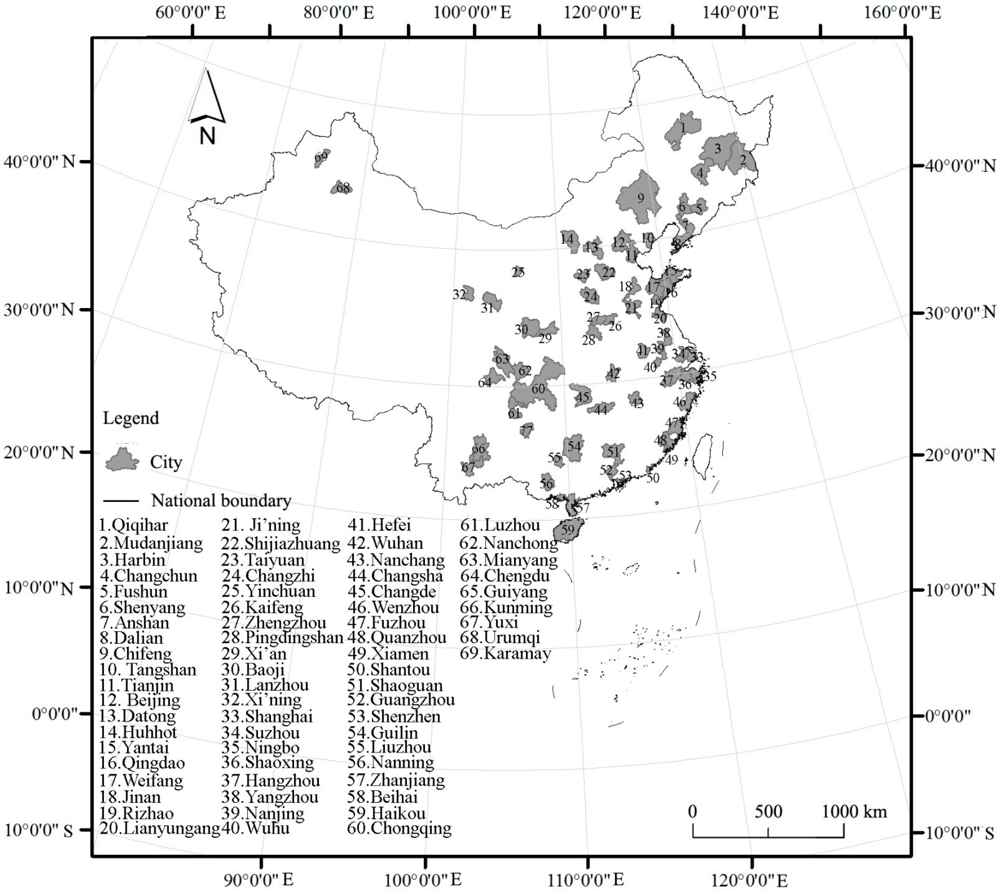
Figure 2.
(a–e) Maps of (a) Air Pollution Index (API) and emissions of (b) PM2.5, (c) PM10, (d) NOx, and (e) SO2 in 69 Chinese cities, 2010.
Figure 2.
(a–e) Maps of (a) Air Pollution Index (API) and emissions of (b) PM2.5, (c) PM10, (d) NOx, and (e) SO2 in 69 Chinese cities, 2010.


Figure 3.
Standardized stepwise regression coefficients for predicting emissions of PM2.5, PM10, NOx, and SO2 based on socioeconomic and urban from factors. ** p-value < 0.01, * p-value < 0.05.
Figure 3.
Standardized stepwise regression coefficients for predicting emissions of PM2.5, PM10, NOx, and SO2 based on socioeconomic and urban from factors. ** p-value < 0.01, * p-value < 0.05.


Figure 4.
(a–e). Standardized coefficients in stepwise regressions for predicting Air Pollution Index (API) based on socioeconomic, climatic, and urban from factors. T = temperature; P = precipitation; RH = relative humidity; W= wind speed; Pop = population; PopD = population density; AWMFD = area weighted mean fractal dimension of built-up area. ** p-value < 0.01, * p-value < 0.05.

Table 1.
Urban form, socioeconomic factors, climatic variables, and air pollution measures considered in this study.
Table 1.
Urban form, socioeconomic factors, climatic variables, and air pollution measures considered in this study.
| Category | Measure | References |
|---|---|---|
| Air pollution measures | Emissions of PM2.5, PM10, NOx, and SO2 | [26,34] |
| Air Pollution Index (API) | [4,35] | |
| Socioeconomic factors | Gross Domestic Product (GDP) | [6] |
| GDP per capita | [22] | |
| GDP of secondary industry | -- | |
| Per capita GDP of secondary industry | -- | |
| Population size | [6,36,37] | |
| Population density | [22,25,36,37,38] | |
| Climatic factors | Temperature | [22,26,30,39] |
| Precipitation | [30] | |
| Wind speed | [6,30,39] | |
| Relative humidity | [30,39] | |
| Sunshine duration | [30] | |
| Urban form metrics | Total built-up Area (TA) | [22] |
| Mean Patch Area (MPA) | [22,24] | |
| Percentage of Landscape (PLAND) | [40] | |
| Patch Density (PD) | [40] | |
| Largest Patch Index (LPI) | [16] | |
| Edge Density (ED) | [16] | |
| Landscape Shape Index (LSI) | [16] | |
| Area Weighted Mean Fractal Dimension (AWMFD) | [16] | |
| Clumpiness index (CLUMPY) | [16] | |
| Aggregation Index (AI) | -- |
Table 2.
Stepwise regression results of air pollutant emissions from different sources in relation to socioeconomic and urban form factors for 69 Chinese cities.
Table 2.
Stepwise regression results of air pollutant emissions from different sources in relation to socioeconomic and urban form factors for 69 Chinese cities.
| Source | Type of Air Pollutant | R | Adj. R2 | F-Value | p-Value |
|---|---|---|---|---|---|
| Industry | PM2.5 | 0.836 | 0.685 | 50.349 | <0.001 |
| PM10 | 0.849 | 0.707 | 55.733 | <0.001 | |
| NOx | 0.884 | 0.771 | 77.102 | <0.001 | |
| SO2 | 0.801 | 0.631 | 59.222 | <0.001 | |
| Power Generation | PM2.5 | 0.546 | 0.277 | 14.022 | <0.001 |
| PM10 | 0.544 | 0.275 | 13.873 | <0.001 | |
| NOx | 0.572 | 0.307 | 16.079 | <0.001 | |
| SO2 | 0.5 | 0.227 | 10.981 | <0.001 | |
| Residential Sector | PM2.5 | 0.683 | 0.441 | 18.894 | <0.001 |
| PM10 | 0.676 | 0.432 | 18.255 | <0.001 | |
| NOx | 0.768 | 0.564 | 23.004 | <0.001 | |
| SO2 | 0.439 | 0.181 | 15.983 | <0.001 | |
| Transportation | PM2.5 | 0.875 | 0.755 | 70.815 | <0.001 |
| PM10 | 0.875 | 0.754 | 70.536 | <0.001 | |
| NOx | 0.874 | 0.757 | 107.001 | <0.001 | |
| SO2 | 0.867 | 0.744 | 99.606 | <0.001 |
Table 3.
Stepwise regression results of API in relation to climatic, socioeconomic, and urban form factors in different seasons for 69 Chinese cities.
Table 3.
Stepwise regression results of API in relation to climatic, socioeconomic, and urban form factors in different seasons for 69 Chinese cities.
| Dependent Variable | R | Adj. R2 | F-Value | p-Value |
|---|---|---|---|---|
| Annual API | 0.665 | 0.408 | 12.704 | <0.001 |
| Spring API | 0.574 | 0.309 | 16.181 | <0.001 |
| Summer API | 0.549 | 0.269 | 9.348 | <0.001 |
| Autumn API | 0.387 | 0.124 | 5.825 | 0.005 |
| Winter API | 0.63 | 0.359 | 10.512 | <0.001 |
© 2018 by the authors. Licensee MDPI, Basel, Switzerland. This article is an open access article distributed under the terms and conditions of the Creative Commons Attribution (CC BY) license (http://creativecommons.org/licenses/by/4.0/).
Share and Cite
MDPI and ACS Style
Liu, Y.; Wu, J.; Yu, D. Disentangling the Complex Effects of Socioeconomic, Climatic, and Urban Form Factors on Air Pollution: A Case Study of China. Sustainability 2018, 10, 776. https://doi.org/10.3390/su10030776
AMA Style
Liu Y, Wu J, Yu D. Disentangling the Complex Effects of Socioeconomic, Climatic, and Urban Form Factors on Air Pollution: A Case Study of China. Sustainability. 2018; 10(3):776. https://doi.org/10.3390/su10030776
Chicago/Turabian StyleLiu, Yupeng, Jianguo Wu, and Deyong Yu. 2018. "Disentangling the Complex Effects of Socioeconomic, Climatic, and Urban Form Factors on Air Pollution: A Case Study of China" Sustainability 10, no. 3: 776. https://doi.org/10.3390/su10030776
Note that from the first issue of 2016, this journal uses article numbers instead of page numbers. See further details here.