Ensuring Efficient Incentive and Disincentive Values for Highway Construction Projects: A Systematic Approach Balancing Road User, Agency and Contractor Acceleration Costs and Savings

Abstract

United States State Highway Agencies (SHAs) use Incentive/Disincentives (I/D) to minimize negative impacts of construction on the traveling public through construction acceleration. Current I/D practices have the following short-comings: not standardized, over- or under-compensate contractors, lack of auditability result in disincentives that leave SHAs vulnerable to contractor claims and litigation and are based on agency costs/savings rather than contractor acceleration. Presented within this paper is an eleven-step I/D valuation process. The processes incorporate a US-nationwide RUC and agency cost calculation program, CA4PRS and a time-cost tradeoff I/D process. The incentive calculation used is the summation of the contractor acceleration and a reasonable contractor bonus (based on shared agency savings) with an optional reduction of contractor’s own saving from schedule compression (acceleration). The process has a capability to be used both within the US and internationally with minor modifications, relies on historical costs, is simple and is auditable and repeatable. As such, it is a practical tool for optimizing I/D amounts and bridges the gap in existing literature both by its industry applicability, integrating the solution into existing SHA practices and its foundation of contractor acceleration costs.

1. Introduction

As a motorist, seeing the “orange barrels” of a construction project is an awful sight. It suggests congestion and stop-and-go traffic are likely ahead equating to frustrating delays. All highway work zones come with a cost to the public through travel delays, vehicle operating costs, crash costs, emissions costs, and/or impacts to nearby projects [1]. To reduce these road user costs (RUCs), increasing both the efficiency and sustainability of the United States’ (US) infrastructure, the US Federal Highway Administration (FHWA) has encouraged US state highway agencies (SHAs) to implement Incentive/Disincentive (I/D) contracting provisions for early project completion.

Although US federal guidelines to determine I/D exist [2], guidance is vague and relies on project engineering judgement versus an all-encompassing, calculation-based I/D price optimization process. These guidelines typically result in SHA I/D valuation practices that are based only the RUC or agency costs and are often ad-hoc versus systematic [3,4]. Ad-hoc practices lead to disincentive values that are neither detailed or defendable. This can open SHAs to litigation from contractors as common law states disincentives can only be true incurred costs, difficult to prove without detailed backup [5]. Alternatively, incentive calculations based on RUCs, agency costs, or both are flawed as they focus on what the acceleration is worth to the SHA and not what it will cost the contractor in additional resource inputs. SHAs do not estimate the cost of a highway construction project by first calculating the benefits to the agency and the public and should not take this approach with I/Ds. Said approach in I/D calculations has led to inefficiently valuated incentive values [6].

This paper adds value to industry, presenting an alternative viewpoint of calculating I/D costs; starting with the actual cost for the contractor to acceleration and build from there. The findings also add to both industry and academia, presenting a detailed, repeatable and auditable I/D process currently nonexistent within literature or SHA practices.

Since the early 90’s, highway researchers and practitioners have developed various models for SHAs to calculate I/Ds. However, even the most holistic SHA models for I/Ds valuations are insufficient [3] with literature finding existing I/D practices lacking due to: (1) no standardized method of valuation, leading to ad-hoc calculations of unknown efficiency [4]; (2) incentive amounts that are unrealistically high, leading the contractor earning a windfall for accelerating costs [6]; (3) incentive amounts are based on agency costs and do not consider contractors cost plus a reasonable profit, providing no attraction for the contractor to accelerate; and (4) disincentive rates are not backed with detailed cost estimations, leaving SHAs vulnerable to litigation [5].

Literature has provided descriptive guidance for SHAs on calculating RUC [7,8,9], construction acceleration cost [4] and maximum and minimums for I/D values [10,11]. However, these tools are only parts of the I/D process and, within literature, there currently exists no holistic process for SHAs follow for calculating an optimum I/D. To fill this gap, this paper presents an eleven-step I/D processes derived from nationwide SHA practices, supplemented through four California DOT (Caltrans) case studies and implemented on a future Caltrans project to validate and compare to existing practices.

To maximize accuracy of I/D calculations, the presented process incorporates a time-cost optimization model, slightly modified from Shr et al. [12] and the Construction Analysis for Pavement Rehabilitation Strategies (CA4PRS) RUC-calculating tool. The process has been developed based on findings from US highway reconstruction and/or rehabilitation projects, though it can be modified to work on international and/or new construction projects. These modifications include replacing the US-based CA4PRS software with something more apt for the international region, and/or changing the method of RUC-calculation for new highway construction. This versatility equates to this paper’s I/D tool being a contribution to both US and international highway practitioners. It is also a contribution to literature as it is an all-encompassing step-by-step I/D calculation process, currently nonexistent in literature.

This paper presents the definition, regulations and use of I/Ds in industry as an understanding of the current I/D state-of practice. The research methods, findings and resultant eleven-step I/D calculation process are then presented. The paper is concluded with a discussion of the processes’ validity through an application on a Caltrans case study project and how contractor’s acceleration costs are calculated.

2. Definition of I/D, Guidelines of Use and Current Practices

2.1. I/D Definition

I/D provisions are designed to shorten the total contract time by giving the contractor an incentive for early completion and a disincentive for late completion. FHWA “Technical Advisory T 5080.10” defines incentives as a contract provision which compensates the contractor a certain amount of money for each day identified critical work is completed ahead of schedule and assesses a deduction for each day the contractor overruns the I/D time. Its use is primarily intended for those critical projects where traffic inconvenience and delays are to be held to a minimum [2]. The amounts are based upon estimates of such items as traffic safety, traffic maintenance and road user delay costs. This definition represents the incentive portion of I/Ds for this paper.

Alternatively, FHWA Technical Advisory defines liquidated damages (LDs) as follows: the daily amount set forth in the contract to be deducted from the contract price to cover additional costs incurred by a SHA because of the contractor's failure to complete all the contract work within the number of calendar days or workdays specified or by the completion date specified [2]. Though the definition is for LDs, it is an apt description of disincentives and represents the disincentive portion of I/Ds for this paper.

2.2. US Guidelines for Determining I/D Amounts

SHAs were first authorized to use I/Ds in the US in 1984 when the FHWA rescinded their policy prohibiting the use of I/Ds. The present FHWA policy is based on the findings of the National Experimental and Evaluation Program Project # 24 which showed that I/D provisions are a valuable and cost-effective construction tool. The typical highway projects that were found appropriate for I/D provisions include projects with high traffic volume in urban areas, lengthy detours created by construction disruption, major bridges out of service, and/or major reconstruction on an existing facility that would severely disrupt traffic [2].

The determination of an appropriate I/D dollar amount is critical for maximizing the potential for project acceleration [2,7]. FHWA suggests that I/D amounts should be based on SHA overhead, traffic control and detour costs along with RUCs on a project-by-project basis. The I/D amount must provide a favorable cost/benefit ratio while covering the contractor’s acceleration costs (based on extended shifts with extra workers for seven days a week). They support the use of engineering judgement for final valuation but suggest that disincentive rates are less than incentive rates with a cap of 5 percent of the total contract [2].

2.3. I/D’s Performance and Current Practices

Using the FHWA and existing literature guidance, I/Ds are being used widely throughout the US using calculation models of differing levels of effectiveness. Through recently published NCHRP-652 report, Fick et al. identified SHAs with extensive experience using time-related I/D projects. Their research indicated that the most of these I/D provisions have been successful at accelerating highway construction work, resulting in reduced delays to the traveling public [6]. A study of 26 Michigan SHA projects also depicted I/D success, finding an average $610,500 savings per project RUC with only a 1.5% increase in the contract amount [13]. A study of 144 Florida SHA projects showed average time savings of 16.5% but average cost overruns of 3.3% for I/D projects in comparison to traditional design-bid-build, non-I/D projects [14].

Although SHAs successfully experience acceleration using I/Ds, they are not optimizing I/D valuation, leading to inefficient spending. Many SHAs’ I/D development procedure are very basic, relying solely on calculated daily RUC amounts for their I/D linear model and only a few include agency costs. Considering the contractor’s cost for schedule acceleration in addition to RUC and agency costs is not universal for any SHA and only performed on a handful of projects. Though these models represent the best-case scenarios for I/D calculations even these were found lacking [3]. They do not take into consideration the contractor’s profit (referenced throughout the paper as a “bonus” and required to effectively incentivize) and lack uniformity across SHAs and even districts with the SHAs [15].

Literature has providing guidance on calculating I/D amounts. Gillespie [7] and Yimin and Irtsihad [9] developed RUC calculating software in their research for Virginia and Florida, respectively. Jiang and Chen [8] developed a cost-time equation to estimate RUCs based on various highway construction processes. While helpful to SHAs, these only discuss one part of the I/D calculation process.

Sillars and Leray [4] took another approach to I/D calculations by presenting the concept that incentive valuations must consider the contractor’s cost of acceleration plus a reasonable profit. The addition of the reasonable profit provides greater incentive to the contractor so that sincere efforts will be made toward accelerating the project. They also propose that the incentive amount be compared to the RUC to make sure the cost to the public of accelerating the project do not exceed the benefits [4]. However, their presentation is merely a concept that relies heavily on engineering judgment. Sillars later presented this concept as a basic boundary equation, Contractor’s Acceleration Cost ≤ I/D ≤ RUC [11].

Shr and Chen took another approach, quantifying a model to determine a reasonable maximum incentive amount based on derived relationship between the construction cost and time duration using Florida highway projects. To determine the maximum days for I/Ds, they developed a curve of the relationship between the construction cost and time duration combined with the I/D line [10]. Alternatively, Shr et al. developed a time-cost tradeoff model to determine I/D values based off of the contractor, RUC and SHA costs [12]. Both of these models aid the SHAs in developing I/D values but they are only a portion of calculating and defending an I/D value (This paper’s process includes a modified and improved version of the Shr et al. [12] curve, described in better detail below).

In summary, there exists no standardized method of I/D valuation in the current SHAs state-of practice [4]. This has led to ad-hoc calculations of I/D values [4], creating incentives that are unrealistically high [6] and disincentive rates that leave SHAs vulnerable to litigation [5]. Previous models in literature have provided solutions but lack applicability as they fail to integrate them into a practical, repeatable and auditable holistic process. SHA I/D practices for calculating I/Ds are also based on the costs to the road users and the agency, with little attention given to the acceleration costs of the contractor. Literature presents the concept of including contractor acceleration costs in I/D valuations but lack any guidance or practical formulas. The model presented in this paper is an evolution of existing practices and literature. It is systematic, repeatable, defendable and provides SHAs clear guidance on creating an I/D based on the contractor’s acceleration costs plus an incentivizing bonus.

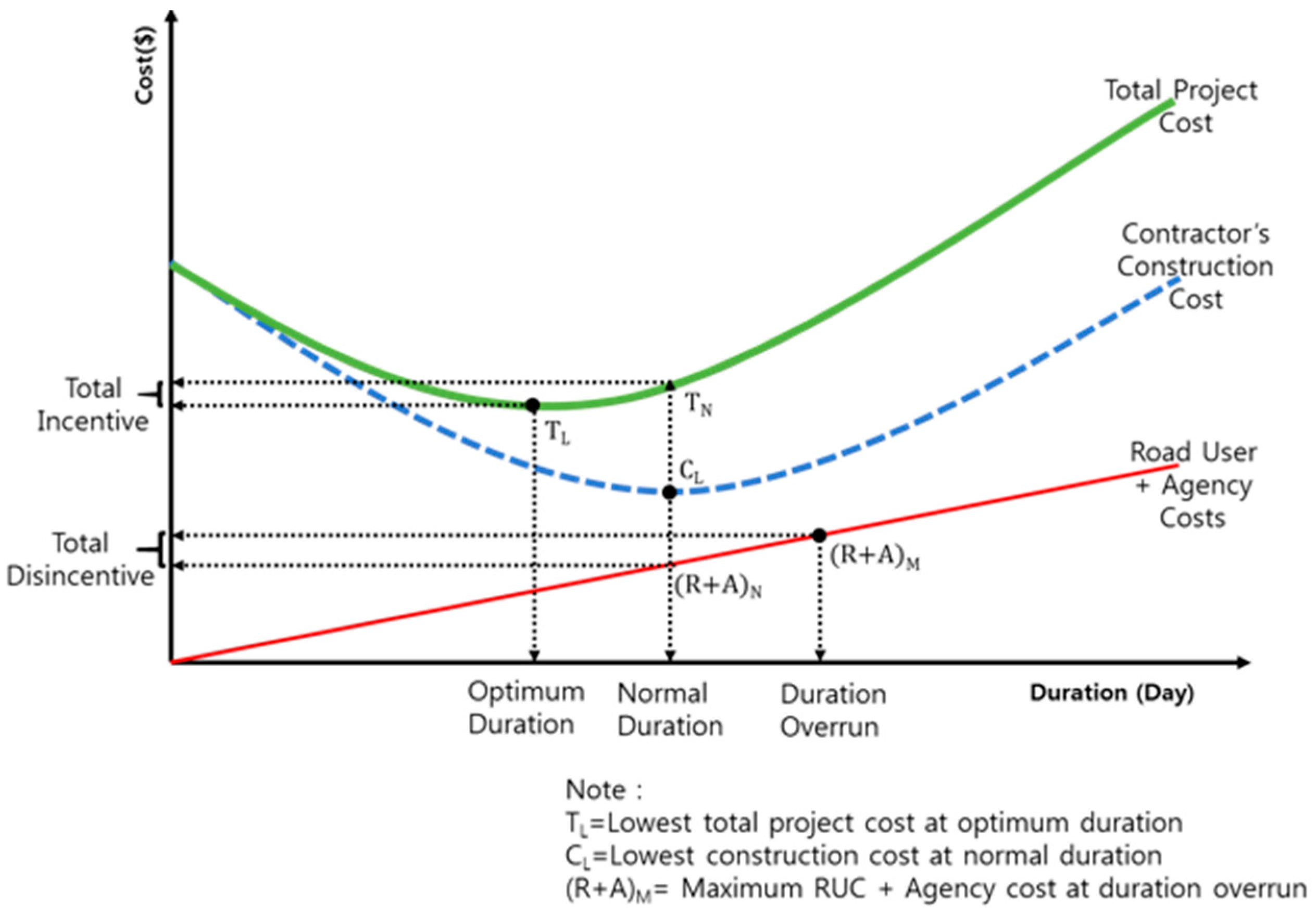
3. Time-Cost Tradeoff Model

Shr et al. developed a time-cost tradeoff model in 2000 which is, to date, the most current model within literature and is therefore an apt framework for this paper’s I/D process (a variation of the model was also published as Shr and Chen [10] and Shr and Chen [16] but only Shr et al. [12] is cited within this paper). Said model is presented in Figure 1 and described in greater detail below.

The developed interrelationship between cost and time shown in Figure 1 was developed through statistical analysis of six Florida projects (R² value of 0.75). The polynomial cost equation, from this regression, representing contractor’s construction costs is simplified by the authors of this paper, as follows [12]:

$$\mathrm{Simplified}\mathrm{CC}=1.006\times {\mathrm{C}}_0-0.10\times {\mathrm{C}}_0\times \frac{\mathrm{D}-0.89\times {\mathrm{D}}_0}{{\mathrm{D}}_0}+0.47\times {\mathrm{C}}_0\times {\left(\frac{\mathrm{D}-0.89\times {\mathrm{D}}_0}{{\mathrm{D}}_0}\right)}^2$$

(1)

where:

• CC = Contractor’s actual project cost
• C₀ = Normal construction cost
• D₀ = Contract time (specified or proposed)
• D = Actual days used by the contractor

Equation (1) was used to develop the dotted line “Contractor’s Construction Cost” curve in Figure 1. On this curve, the normal point is the construction duration at which the construction cost is the lowest [17] and the winning proposal value for completion of a given project. Any variation from the normal point equates to an increase in construction cost (acceleration due to compressed duration and increased overhead due to extended duration [18]). Alternatively, the “Road User + Agency Costs” line, shown in red in Figure 1, is calculated as:

$$\mathrm{Total}\mathrm{Cost}\mathrm{for}\mathrm{duration}\mathrm{D}=\left[\mathrm{RUC}+\mathrm{A}\right]\ast \mathrm{D}+\mathrm{CCD}$$

(2)

where:

• A = Agency Cost
• CCD = Construction Cost at duration D.

The “Total Project Cost” curve is the summation of the contractor cost, RUC and agency costs. This curve initially dips (cost initially decreasing due to reduced contractor’s construction cost) until the ever-increasing RUC and agency overhead costs negate the savings received from reduced contractor’s construction cost. This minimal point represents the cheapest option for the agency and the optimum duration. The optimum and normal duration’s cost/duration intersection points are used to calculate the daily incentive (based on total cost) rate as shown in Equation (3):

$$\mathrm{Daily}\mathrm{Incentive}\mathrm{rate}(\$/\mathrm{day})=\frac{\mathrm{Total}\mathrm{Incentive}(\$)}{\mathrm{Optimal}\mathrm{Acceleration}\mathrm{Duration}\left(\mathrm{days}\right)}$$

(3)

where:

• Total Incentive = TN – TL
• TN = Total Cost at “Normal duration”
• TL = Total Cost at the “Optimum duration”
• Optimal Acceleration Duration = (Normal duration – Optimum duration).

The Daily Incentive rate in Equation (3) does not consider the quantifiable acceleration costs of the contractor with needed critical resources arrangement and has the potential to result in an inefficient or ineffective I/D. This is a shortcoming within literature the I/D process presented below includes an I/D adjustment step which is based on the daily contractor acceleration costs. From the same time-cost model, a daily disincentive rate can be calculated as follows:

$$\mathrm{Daily}\mathrm{Disincentive}\mathrm{rate}\left(\$/\mathrm{day}\right)=\frac{\mathrm{Total}\mathrm{Disincentive}(\$)}{\mathrm{Delay}\mathrm{Duration}\left(\mathrm{days}\right)}$$

(4)

where:

• Total Disincentive = (R + A)_M – (R + A)_N
• (R + A)_M = RUC + Agency costs at “Duration Overrun”
• (R + A)_N = RUC + Agency costs at “Normal Duration”
• Delay Duration = Overrun (SHA Specified) – Normal Duration

Although the above equation is accurate, it can be simplified in most cases. This is because the RUC and Agency costs are most commonly linear. When the RUC and Agency costs are the same for every day (linear), the following equation can be used:

$$\mathrm{Daily}\mathrm{Disincentive}\mathrm{rate}\left(\$/\mathrm{day}\right)=\mathrm{RUC}+\mathrm{Agency}\mathrm{Cos}\mathrm{t}$$

(5)

4. Point of Departure and Contributions to Practice and Theory

Reviews of current US SHA practices in calculating I/D amounts have been found to be lacking, often ad-hoc or overly-simplistic, mainly due to the lack of a systematic, replicable and auditable process [3,4,5,6]. This paper develops an all-encompassing step-by-step I/D calculation process, with some improvement and enhancement of the Shr et al. [12] model, that is replicable, auditable and currently nonexistent in literature. The presented process is beneficial to both US and international highway practitioners as it can be modified to work in any region. Beyond the step-by-step process itself, this paper also contributes by filling another research void, presenting a formula and guidelines for calculating an I/D based on contractor acceleration. Finally, the process includes using the RUC-calculation tool, CA4PRS, which is allows for more accurate costs to the agency than previously-cited I/D RUC calculation methods.

5. Research Methods

The objective of this paper is to develop an optimum I/D daily dollar amounts calculation process that can be easily integrated into SHA practices. To address this objective, the authors:

(1)

Performed a literature review related to determining daily I/D dollar amounts and up-to-date information on current practices to set up I/D amounts;

(2)

Collected Caltrans I/D project data, including project type and location, construction time and cost information, average daily traffic (ADT), project length, I/D daily dollar amounts and maximum incentive cap amounts;

(3)

Collected I/D project data nationwide from 291 sampled projects collected through an FHWA alternative contracting methods cost/benefit investigation;

(4)

Performed loosely structured interviews with subject matter experts from eight public/industry agencies and one screen survey with multiple SHA representatives;

(5)

Evaluated performance of projects collected in steps 3 and 4 above, specifically the relationship between I/D dollar amount and project time and cost performance;

(6)

Evaluated RUC-calculating computer simulation software;

(7)

Performed case studies on four Caltrans I/D projects, performing I/D calculations using three different levels of CA4PRS implementations for said calculation; and

(8)

Demonstrated tool implementation on one Caltrans project.

The research methodology is presented in Figure 2 below with the above research method numbers referenced. An abbreviated summary of the relationships are as follows: (a) the literature review aided the software analysis; (b) the data collection pursuits resulted in a project database and selection of subject matter experts; (c) from the project database the project case studies and implementation project were chosen and a quantitative analysis was performed resulting in a project performance database; and (d) the findings from the literature review, interviews, project case studies, software analysis and performance database resulted in the I/D process which was (e) implemented on one potential future Caltrans project. A description of each research methodology can be seen below.

5.1. Literature

The FHWA has supported the use of I/Ds since the early 90’s. As such, there have been many research endeavors dedicated to their use, performance and development. The researchers performed a holistic review of I/D literature within the American Society for Civil Engineers (ASCE, Reston, VA, USA) online library, Transportation Research Board (TRB, Washington, DC, USA) online publications and a Google Scholar search for the key words incentive and disincentive. The relevant findings have been presented above.

5.2. Caltrans I/D Project Data Collection

The researchers performed a review of Caltrans development practices, finding a total of 48 I/D projects awarded within 2003 and 2010. The researchers reviewed the data of these projects and found, 43 I/D projects completed in 11 districts apt for this study and used them for data analysis. The project characteristics are as follows:

• Most of the projects were 3R projects (resurfacing, rehabilitation and reconstruction) or widening;
• 23, or 54%, of the projects had high traffic volumes;
• Median project length was 3.8 miles;
• Average contract award was approximately $40 million;
• Average duration was 515 working days;
• Average incentive cap was $1.1 million per project, ranging from $15,000 to $5.3 million;
• 22 projects’ incentives were between $100 and $600 k.

5.3. FHWA Nationwide I/D Project Data Collection

As a part of an FHWA nationwide study on the costs, benefits and risks of using alternative contracting methods, the researchers investigated the I/D practices used by differing projects within multiple SHAs. Of the 279 projects in which the agency representative stated they were able to answer I/D questions, 76 (27%) stated they used some form of incentives and/or disincentives (or LDs) in an attempt to accelerate the project. Of those projects, 67 answered the components they used for calculating their I/Ds. This included 30 design-bid-build, 23 design-build and 14 construction manager-general contractor in 19 state and federal agencies completed between 2004 and 2015. The award values ranged between $1 to $334 million. The questions within the survey pertaining to this research included: delivery method, I/D amount available to contractor, I/D amount earned by the contractor and what components were included in the I/D valuation.

5.4. Subject Matter Expert Interviews

Loosely structured interviews were performed with multiple subject matter experts concerning I/D valuation best practices. The researchers interviewed representatives from eight public/industry agencies from California, including: Caltrans, Orange County Transportation Authority, Riverside County Transportation Department, San Bernardino County Department of Transportation, American Concrete Pavement Association (California chapter), National Asphalt Pavement Association (southern California chapter) and two consultant companies, PB Consulting Group and CH2M Hill. These interviews took place via face-to-face, phone, or email. The discussions included how the I/Ds were developed, what tools and processes were used, how efficient the I/D values were and any suggestions of improvement as relevant depending on the interviewees experience. From these discussions, a I/D process the incentive adjustment equation, shown as Equation (7) below, began to evolve. In an attempt to supplement the California-based interviews with national practices, the researchers invited subject matter experts involved with the FHWA alternative contracting methods study for a screen survey to present, discuss and further develop the model. It should be noted that the core research team also included subject matter experts with experience as follows: 20 years alternative contracting research experience, 20 years RUC highway research and modelling experience and 30 years highway industry experience. The research team’s own input and experience aided in the development of the final product.

5.5. Quantitative Analyses

Several correlation analyses were performed to identify any relationship between the incentive amount and original schedule performance, original cost performance, project award and annual daily traffic (ADT). Statistical analysis was also performed on a small sample size of projects. The results of these studies informed the I/D process development but are not directly pertinent to this paper. Said findings can be found in Pyeon and Lee’s final research report [19] and upon request from the FHWA research team (as I/D quantitative analyses findings were unpublished) [20].

5.6. Computer Simulation Software for Lane Analysis and Potential Road User Impacts

The researchers incorporated a computer simulation tool for analysis of the work zone impacts into the I/D process. While being the current state-of-practice for many SHAs [21], a computer simulation model also brings uniformity to RUC, agency costs and the lane closure scheme calculations [22]. In a study on the implementation of work zone simulation models for New England projects, Collura et al. [21] found CA4PRS one of four apt models for projecting construction work zone impact on road users (CA4PRS was developed by the Institute of Transportation Studies at the University of California Berkeley).

The author chose to incorporate CA4PRS, versus competing models, as it has been formally and nationally promoted by FHWA and has gained nationwide acceptance (18 states having license and training and 12 states interested in license and training as of 2010). The CA4PRS tool was also specifically developed to aid SHAs in valuating I/Ds through RUC calculation. Therefore, the CA4PRS provides I/D valuation best-practices currently being executed by SHAs. These practices were used as a baseline for the researcher’s development of the I/D eleven-step process presenting within this paper. The CA4PRS program includes a schedule module that calculates duration, a traffic module that calculates duration and impact of work zone lane closures and a cost module that estimates agency costs. These capabilities of the CA4PRS tool has been confirmed on several major highway rehabilitation projects in states including California, Washington and Minnesota [23].

As the I/D process is primarily based on the calculation of RUCs, a brief discussion of how the CA4PRS model calculates them follows. SHAs most commonly use a Demand-Capacity model for calculated the RUCs. This calculation uses road user demands on the road to be worked on, based on historical data and road capacity estimated using the Highway Capacity Manual (formulas found in Chapter 29 of the HCM 2000) [24]. Using these variables, the road user delays (vehicle-hours) are estimated by comparing the accumulated demand and capacity curves. The road user vehicle-hour delays are multiplied by the summation of the vehicle operating costs and crash costs incurred resulting from lane closures, resulting in the work zone RUCs. The CA4PRS Demand-Capacity model is coded with Visual Basic and access a MS Access database to calculate the work zone traffic delays in terms of queue length per closure equating to RUCs [25].

5.7. Caltrans I/D Implementation Case Studies

The four case study projects descriptions can be seen below in

Table 1. Case Study Project Characteristics.

Project	CA4PRS Stage Used	Project Characteristics (PC), Incentive (I), Disincentive (D), Earned (E)
I-10 Pomona	Schedule Analysis (1)	PC:	Long-life concrete rehabilitation project; 240,000 ADT, 9% trucks
		I:	$600 per lane-m replaced >2000 lane-meters during closures $500,000 Maximum
		D:	$250 per lane-m replaced <2000 lane-meters during closures $10,000 per 10-min of lanes still closed on Monday morning
		E:	The contractor was awarded $500,000
I-710 Long Beach	Schedule Analysis	PC:	Long-life concrete rehabilitation project; 164,000 ADT, 13% trucks
		I:	$100,000 per weekend closure <10 weekend closures $500,000 Maximum
		D:	$100,000 per weekend closure >10 weekend closures
		E:	The contractor was awarded $200,000 (8 weekend closures)
I-15 Devore	Traffic Analysis (2)	PC:	4.5 km truck lanes rebuild; peak 5500 vehicles/h and 110,000 ADT
		I:	$300,000 if closure was completed faster than 111 h per unit $75,000 per day completed faster than 19 days
		D:	Uncapped $ if closure was completed slower than 111 h per unit $75,000 per day completed slower than 19 days
		E:	N/A
I-80 Sacramento *	Schedule, Traffic, Cost Analysis (3)	PC:	8.6 miles Rehab with widening; 140,000 ADT and estimated 200,000 ADT by 2030 with 10% trucks
		I:	$100,000 per reduced weekend closure $400,000 Maximum
		D:	$100,000 per increased weekend closure
		E:	N/A

⁽¹⁾ CA4PRS was used for the staging and lane closure plans. RUCs are incorporated through the schedule estimate and work zone traffic analysis of CA4PRS. ⁽²⁾ CA4PRS developed baseline schedule, staging and lane closure plans, work zone traffic analysis and estimated RUCs. ⁽³⁾ CA4PRS developed baseline schedule, staging and lane closure plans, work zone traffic analysis, and estimated RUCs. Only one-third of the RUCs were factored into the I/D calculations, a commonly used practice in other states. * At the time of this study, the I-80 Sacramento project was in initial planning stages. Therefore, I/D amounts are not actual but the calculated suggestions.

below. Shown are the stages in which CA4PRS was used along with the project characteristics, I/D amounts and the amount earned by the contractor.

5.8. Demonstration of Implementation on a Caltrans Project

As a way to both validate the effectiveness of the tool and to better illustrate its use, the authors have implemented the eleven-step process using the I-15 Ontario future highway pavement resurfacing. The I-15 Ontario project includes a 12″ PCC slab and 6″ AC replacement, about 10.5 lane-mile pavement reconstruction with 3 lanes each direction. The calculated ADT was 105,000 and there are 8-h nighttime closures expected with the lane closure one lane open to traffic and 2 lanes for construction and access. CA4PRS was used for full schedule, traffic and cost analyses.

6. Optimum ID Process with Step-by-Step Procedure

6.1. Findings from Existing SHA Practices

Through the performed Caltrans case studies, it was discovered that, as in literature, the most common I/D amount calculation was RUC. Within the FHWA project database, the researchers found much of the same. Forty-two percent of SHA projects only used RUC, 14% only used the SHA’s cost, 2% used the contractor’s cost, 11% used the project acceleration cost and 18% used the SHA policy. Only 14% used a combination of the RUC, SHA and contractor costs as is recommended within literature. These findings are represented below in

Table 2. FHWA I/D Valuation Findings.

I/D Valuation Component	No.	Percentage
Road User 1	28	42%
SHA 1	9	14%
Contractor 1	1	2%
Project Acceleration 1	7	11%
Some Combination of Above	9	14%
Only SHA Policy	12	18%
None of the above	1	2%

¹ Some respondents claimed using these valuation components with policy or other (ex. SHA and policy, contractor and other). The researchers felt the policy and other valuations were secondary components and therefore labeled these dual responses only as the primary valuation component (ex. the researchers are presenting a SHA and policy response as SHA).

. (It should be noted this data comes only from SHAs using design-build and/or construction manager/general contractor delivery methods. While the researchers feel this is an apt representation of SHA practices, it is not statistically representative of the entire population, all executed projects in the US).

However, even the more-encompassing I/D calculation projects were lacking. For SHAs to have a more comprehensive and effective I/D amount calculation, it is necessary to broaden the I/D amount calculation criteria covering realistic cost items, as suggested in this paper with the optimum I/D Process below. Items needing to be considered, that are not currently common practice, include the agency’s administrative cost savings (resulting from the reduction of road closures) and contractor’s overhead cost savings associated from reducing project duration.

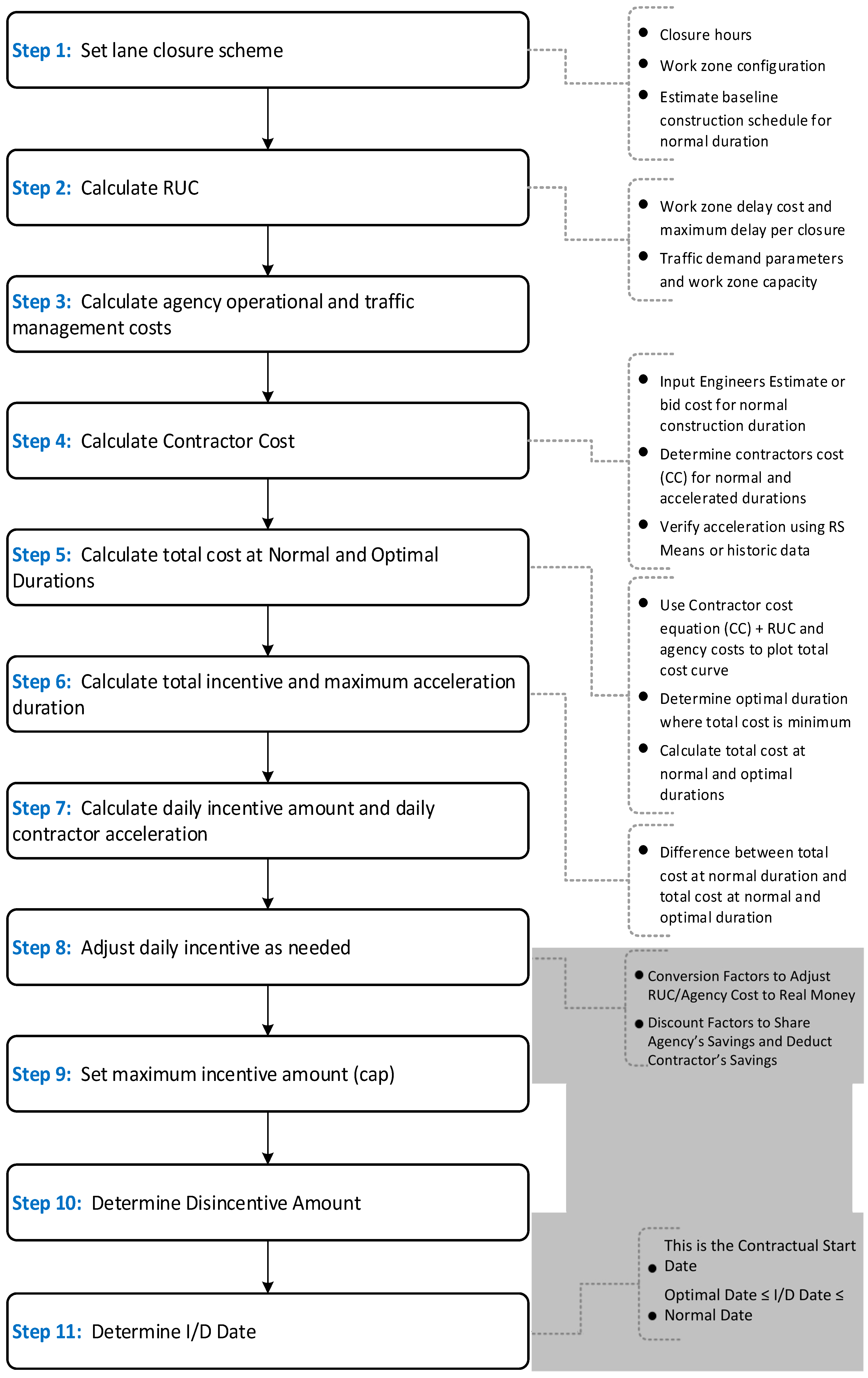
6.2. Step-by-Step Procedure for Optimum I/D Process

Based on the findings of the case studies and performance surveys, a more systematic procedure needs to be developed for SHAs to set up efficient I/D values. This approach should consider the given project conditions considering the costs/benefits to the agency, contractor and users. Thus, the researchers developed an initial framework for developing systematic procedures of I/D amounts. From literature and case study best practices, the researchers developed the following proposed I/D amount assessment procedures, broken down into four criteria:

• Traffic Impacts: analyze work zone impacts, check if acceleration through incentive is feasible and estimate RUC.
• Schedule Analysis: Estimate baseline schedule, identify contractor’s major constraints on critical activities, identify contractor resources required for acceleration and calculate maximum schedule compression.
• Cost Estimate: Estimate contractor’s cost for additional resource inputs, agency cost benefits and contractor’s benefits for schedule compression.
• I/D Amount Calculation and Adjustments: calculate minimum daily incentive (contractor cost for acceleration), baseline daily incentive (contractor additional cost, RUC savings, agency cost savings, less contractor’s savings), maximum daily incentive (RUC plus agency cost savings) and incentive cap (incentives * maximum compression). I/Ds amounts within the calculated range

Alternatively, CA4PRS has the following procedures to determine an I/D dollar amount:

• Schedule Baseline

  ○

  Inputs: closure options, section profile, lane width, curing time and working method

  ○

  Outputs: detailed schedule with construction window types and closures

• Estimate impact of the work zone on the traveling public:

  ○

  Inputs: roadway capacity and traffic information

  ○

  Outputs: work zone user delay costs

• Chose a conversion factor to discount the value of the RUC and agency cost

  ○

  Input: conversion and discount factors

  ○

  Output: I/D dollar amount per closure

• Set up the maximum incentive amount

  ○

  I/D dollar amount per closure and schedule baseline

  ○

  Maximum incentive and number of closures

From these initial procedural guidelines, the researchers developed an eleven-step I/D calculation process shown Figure 3 and detailed below. This logical process includes incorporating contractor’s daily acceleration costs with additional critical resources and even optionally contractor’s overhead cost saving from their own acceleration (schedule compression), which has not been represented in literature or SHAs best practices.

The following describes the inputs, outputs and actions of each step within the eleven-step I/D process shown above.

Step 1: Set Closure Scheme. In this step, the SHA estimates the baseline construction schedule and the lane closure scheme (lane closure frequency, duration and strategies). SHAs typically develop the estimated baseline schedule using production rates, predetermined job logic, or an integrated scheduling system which combines the two [26]. The CA4PRS program (Schedule Analysis module) is very effective at calculating the closure schemes but can also be used to calculate the estimated baseline schedule. The duration will eventually be used as the normal duration in future steps (especially Step 5).

Step 2: Calculate Typical Daily RUC. Using the closure scheme, the SHA calculate the typical daily RUC. This process includes the closure scheme findings, work zone lane capacity based on highway capacity manual procedure, traffic demand parameters and their sensitivity and the time value for traffic delays (per hour per vehicle). Inputting this information into the CA4PRS program (Work-Zone Analysis module), the SHA will have a RUC cost per workday closure and total expected RUC for the entire project. The SHA may wish to use a discount factor for the conversion of RUCs, which is discussed below in Step 8.

Step 3: Calculate Daily Agency Cost. Whether the contractor accelerates critical work completion or extends it, it will impact SHA’s field management costs. Therefore, the daily agency cost must be taken into consideration in I/D development. The field management costs typically include the resident engineer, field engineer, inspector, traffic engineer, material testing, construction zone safety, traffic management plan costs, etc. This step is straight-forward, requiring knowledge of agency costs.

Step 4: Calculate Contractor’s Cost. This step is already performed by all SHAs on every project as the engineering estimate. This value is the normal construction cost (C₀) based on a normal duration (D₀) in Equation (1). If a SHA-specific model is developed, as seen in Equation (1), the SHA will use said model to plot the contractor construction (CC) cost curve. The model developed by Shr et al. [12] is used with some modification and enhancement for this paper but a SHA can also develop the cost curve performing CC cost calculations for the reasonable range of durations in whatever format available to them (this could be resource intensive). Either way, this is performed by inputting project durations (D) into Equation (1) ranging from approximately 2/3 to 4/3 the D₀ duration (200 and 400 for a normal duration of 300). Though the extreme durations are unrealistic, this range will allow for a full development of the CC cost curve.

Step 5: Calculate Total Cost at Normal and Optimal Durations. After plotting the CC cost curve, the total cost at normal duration (TN) and the total cost at the optimal duration (TL) are calculated. Using Equation (2), the SHA plots the RUC and agency curve for the same range of durations as the CC cost curve. TN is found by calculating and adding the CC, RUC and agency costs at the normal duration. Conversely, the TL is found by calculating and adding the CC, RUC and agency costs at the optimal duration (minimum total cost).

Step 6: Calculate Total Incentive and Maximum Acceleration Duration. As seen in Equation (3), the TN and TL are used to calculate the total incentive and maximum acceleration. The maximum acceleration duration to be offered to the contractor is the duration between the normal and optimal duration. The total incentive to be offered is the difference between TN and TL. TN represents the lowest cost of the combination of the CC, RUC and agency cost. Acceleration past the duration at TN begins to increase the total cost and is undesirable. For this fact, the duration at TN acts as a maximum incentive boundary.

Step 7: Calculate Initial Daily Incentive and Contractor Daily Acceleration Cost. The initial daily incentive cost is calculated by dividing the total incentive amount by the maximum acceleration duration (Equation (3)). This incentive value is for the SHA’s reference but should not be used as it does not incorporate the contractor’s acceleration costs (actual daily incentive is calculated in Step 8). The contractor daily acceleration should also be taken into consideration. The authors used the following daily contractor acceleration formula based on contractor’s cost calculated in Equation (1):

$$\mathrm{Daily}\mathrm{Contractor}\mathrm{Acceleration}\mathrm{Cost}=\frac{C{C}_{Optimal}-C{C}_{Normal}}{\mathrm{Optimal}\mathrm{Acceleration}\mathrm{Duration}\left(\mathrm{days}\right)}$$

(6)

where:

• CC_Optimal = Equation (1) result using the optimal point cost and duration
• CC_Optimal = Equation (1) result using the normal point cost and duration
• Optimal Acceleration Duration = (Normal duration − Optimum duration)

If the SHA desires a more accurate contractor acceleration charge and has the resources to dedicate to it, the authors suggest using commercial cost estimating database such as the RS Means heavy construction database to develop an estimate for the contractor’s acceleration charges. The crew cost data from RS Means can accurately provide SHAs detailed cost impacts that changes in duration have on crew and material costs [11] and is therefore very useful for calculating contractor acceleration. The SHA should also calculate the contractor’s estimated cost savings due to schedule compression. Once again, this can be calculated through RS Means and will be used when considering the final I/D values. The process of calculating contractor acceleration is presented in greater detail in Section 6.4 below.

Step 8: Adjust Daily Incentive with Conversion and Discount Factors. SHAs and literature currently have no tool or formula to develop a daily incentive amount based on contractor acceleration. This is where this paper adds significant value. To aid SHAs in developing an efficient I/D amount, accurately set, SHAs should use the formula, as suggested by the authors:

$$\mathrm{Daily}\mathrm{Adjusted}\mathrm{Incentive}\mathrm{rate}\left(\$/\mathrm{day}\right)=CA+SharedA-CAsavings\left(optional\right)$$

(7)

where:

• CA = Daily Contractor Acceleration Costs
• Shared Agency Savings (Shared A) = $\frac{\frac{\mathrm{RUC}}{C{F}_1}+\frac{AgencyCosts}{C{F}_2}}{{\mathrm{DF}}_1}$
• CA savings = $\frac{{\mathrm{Contractor}}^{\prime }\mathrm{s}\mathrm{overhead}\mathrm{savings}\mathrm{from}\mathrm{acceleration}}{{\mathrm{DF}}_2}$
• CF = Conversion Factor
• DF = Discount Factor
• CF₁ = range of 1 to 3
• CF₂ = range of 1 to 2
• DF₁ = range of 2 to 3
• DF₂ = range of 5 to 10

As can be seen, this calculation is set up so that the incentive rate will compensate the contractor for their acceleration costs, plus a bonus as share of agency savings and benefits. This formula’s foundation is Sillars’ [11] discussion that the I/D value should be greater than the contractor’s acceleration costs but less than the agency savings, represented as RUC. The authors of this paper know that the agency’s savings also include agency overhead costs and have added “agency costs” to the shared agency savings portion of the calculation. The authors have also added a contractor savings portion that reduces the I/D value, increasing its efficiency and ensuring the contractor is not overcharged.

Step 8.1: Discount Factors. Discounting RUC costs is a common occurrence that is cited in literature [1,19]. This is because I/D valuations are typically only based on the RUC. This paper presents a case that this is an insufficient practice and the I/D should include the contractor’s acceleration, RUC and agency costs and optionally a deduction of the contractor’s overhead savings. However, no literature or SHA guidelines provide any suggestion on how to properly calculate the I/D with all of these factors. Based on literature review and case studies but mainly discussions with subject matter experts, the authors developed Equation (7) seen above. This formula relies heavily on conversion and discount factors. The conversion factors are used as a way to reduce the “soft-money” RUC and SHA costs (costs that are incurred beyond the project, examples are inconvenience to the public and agency staffing) to “hard-money” (the costs actually borne by the project). The discounting factors are used for the agency to control how much of the acceleration savings they are willing to share with the contractor.

For the conversion factors, CF₁ converts the inconveniences cost of the public to project hard-costs (ex. increasing traffic safety). Similarly, CF₂ converts the agencies cost savings which is a combination of hard-money (ex. traffic control) and soft-money (agency overhead paid regardless of the job). SHAs typically use conversion (sometimes called discount factors as well) factors between 1 and 5 to discount RUC and/or agency costs [1,19]. As can be seen in Equation (7), CF₁ is suggested to be between 1 to 3 and CF₂ between 1 and 2. Once converted to hard-costs the agency uses DF₁ to keep a portion of the fiscal benefits of the acceleration, rather than transferring all these benefits to the contractor. This is suggested to be between 2 and 3.

Concerning values the SHAs may chose, as a general rule the conversion factors should be 1 on low-trafficked roadways, defined as less than 50,000 by Fekpe et al. [27]. Alternatively, if the project is a highly-trafficked roadway (100,000 ADT+), conversion factors should be 2. The authors suggest that DF₁ should be 2 on low-trafficked roadways and 3 on highly-trafficked roadways. Finally, only on mega-projects with an urgent need for early lane closure completion should the CF₁ be 3, as it is likely on these projects that the RUC is very high.

Please recall that Equation (7) is fundamentally different than existing I/D calculations processes. In both literature and practice the incentive calculation is based solely on the RUC and/or agency cost and so only a conversion from soft- to hard-costs is required. Alternatively, Equation (7) is based off of contractor acceleration, adding a Shared Agency Savings and optionally reduction of contractor’s overhead saving from acceleration. Therefore, the RUC and Agency Savings are first converted to hard costs and then adjusted (discounted) to ensure the agency does not release all shared savings to the contractor.

Step 8.2: Contractor Savings. The final variable of Equation (7), contractor’s savings, is optional and an advanced form of calculating I/Ds. In reducing the incentive rate by the value of contractor’s savings, the SHA is showing an effort to fairly reduce the bonus earned by contractors to a reasonable level. If this is not reduced, the contractor could earn the savings of acceleration without an equivalent reduction in incentive payment. However, if an agency is uncomfortable with the accuracy of their calculation there could be a concern that this reduction would reduce the incentive to a value only compensating the contractor’s daily acceleration costs (reducing incentive effectiveness). Therefore, the contractor savings should only be used by SHAs with a history of using detailed I/D calculation processes resulting in contractor acceleration, RUC and agency cost calculations that they are comfortable are highly accurate. For highly trafficked projects with intensive lane closures scheme over relatively short-term, it is suggested a higher value (DF₄ = 8 to 10) is used (i.e., meaning less incentive reduction for the contractor’s own saving from their schedule acceleration). The lower values (DF₄ = 5 to 7) should be reserved for the mega-projects such as capital corridor widening projects where the contractor is able to achieve some saving in their overhead cost from feasible schedule acceleration in the long run.

Step 8.3: Summary. It should be noted that these values are based on limited interviews and are “rules of thumb” guidelines. These discount factors could be very politically charged (too low DFs may be controversial as the contractor would be over-paid) or result in no acceleration (too high DFs may not compensate the contractor enough). Equation (7), specifically the variability in the discounting factors, in Step 8 admittedly reduces the exactitude of the presented I/D process.

As a sensitivity example of the conversion and discount factors in Equation (7) above, if a CF₁ of 2 is chosen, the RUC value (saving) will be converted (reduced) in half and therefore the daily adjusted incentive will also be reduced by half of the RUC value. As a combination case, when CF₁ = 2, CF₂ = 2, DF₁ = 2, DF₂ = 2, only a quarter (25%) of the RUC and agency cost values are added to the incentive value (2 × 2 = 4, RUC and agency values are divided by 4) as shared agency savings and half (50%) of the contractor’s overhead saving from its acceleration is reduced from the daily incentive amount. Though this seems simple, the authors wanted to illustrate that the CF₁/CF₂ and DF₁ variables probably should not be chosen in isolation as their combination is ultimately what determines how great the savings the agency wishes to share is reduced.

Due to the high variability in project types, the authors felt they could not totally remove engineering judgment in the I/D valuation process. SHAs still need to perform research of their own to set up reasonable guidelines that best suits their region and risk culture. However, the presented eleven-step I/D valuation process still contains a great deal more detail, instruction and guidance to SHA representatives than any I/D process existing in highway literature or practice.

Step 9: Set Maximum Incentive Amount. The maximum incentive amount should be that which was calculated in Step 6. However, based on the FHWA guideline for maximum incentive (i.e., 5% cap) most SHAs use a fixed amount, fixed percent of construction cost, or flat-rate dollar amount as the maximum incentive [2,10]. The SHA should set the maximum incentive as that calculated in Step 6 or the agency budget limit, whichever is less. If the maximum incentive is set by SHA policy and is less than the desired calculated total incentive, the agency still has an optimized incentive value with the greatest potential for encouraging contractors to accelerate. However, they remove the potential to reach the optimal point, seen in Figure 1.

Step 10: Determine Disincentive Amount. The penalty clause disallows enforcement of a disincentive if its purpose is to punish the contractor [13]. Legally, a disincentive can only reimburse the agency for incurred expenditures. Therefore, the daily disincentive should be calculated as the daily RUC plus the daily agency cost, seen in Equation (5). However, attention needs to be paid as to what is included in the LD calculations to ensure contractors are not being “double charged” for SHA costs [6]. The maximum disincentive should be as set by the SHA rules and regulations.

Step 11: Determine I/D Date. The final step in this process is to set the I/D completion date. The SHA will pay the contractor in the amount of the previously calculated daily incentive for each calendar day the actual completion date of the critical work item proceeds the I/D completion date. The setting of this date should be based on a reasonable schedule. A SHA may wish to ensure schedule acceleration by setting the contract date as low as the optimal duration. Alternatively, the SHA may wish to rely solely on the incentives to receive schedule acceleration. Either way, the I/D completion date must be greater than or equal to the date of optimal duration and must be less than the date of normal duration. If the SHA sets the I/D lower than the normal duration (especially if significantly lower), a reassessment should be made to the maximum incentive value. This is to ensure that the agency is not paying for the contractor to accelerate to a duration less than the optimal duration. The SHA should also verify that the I/D date represents a reasonably accelerated schedule using historical production data. The CA4PRS program, or similar, can be used to demonstrate the sensitivity of the contractor’s crew size on construction acceleration and pricing.

6.3. Implementation of the Process

In order to test the process’s accuracy versus the current SHA best practices and to better illustrate how the process works, the authors implemented the eleven-step process on the I-15 Ontario potential project. Using the CA4PRS software schedule analysis, work zone RUC calculation and agency cost analysis and the Equation (1) analysis, the authors developed the time-cost trade-off curve graph (Figure 4) and have the findings in

Table 3. I-15 I/D Eleven-Step Process Results.

Step	Resultant
Step 1: Closure Scheme	CA4PRS Output:	8-night time closures 1 lane will always be open 2 lanes closed for construction
Step 2: Daily RUC	CA4PRS Output:	$10,850/day
Step 3: Daily Agency	CA4PRS Output:	$7309/day
Step 4: Contractor Cost	CA4PRS Output:	C0 = $30 Million (Normal Construction Cost)
	Time-Cost Curve:	See above Figure 4.
Step 5: Cost at Normal and Optimal Durations	CA4PRS Output:	D0 = 300 days (Normal Construction Duration)
	Time-Cost Curve:	TN = $35,447,906 (Total Cost at Normal Dur., 300 days) TL = $34,916,974 (Total Cost at Optimal Dur., 242 days)
Step 6: Total Incentive	Time-Cost Curve:	Total incentive (TN – TL) = $530,932 Maximum Acceleration (300 – 242) = 58 days
Step 7: Daily Incentive	SHA Practice:	$\frac{\mathrm{RUC}}{D{F}_1}=\frac{\$10,850}{2}=\$5425/day$
	Time-Cost Curve:	$\frac{\mathrm{Total}\mathrm{Incentive}(\$)}{\mathrm{Optimal}\mathrm{Acceleration}\mathrm{Duration}\left(\mathrm{days}\right)}=\frac{\$530,932}{58}=\$9154$/day
Step 7: Contractor Acc.	SHA Practice:	Not Taken into Consideration
	Time-Cost Curve:	$\frac{C{C}_{Optimal}-C{C}_{Normal}}{\mathrm{Optimal}\mathrm{Acceleration}\mathrm{Duration}\left(\mathrm{days}\right)}=\frac{\$30,522,427-\$30,000,000}{58}=\$522,527=\$9007/day$
Step 8: Adjust Incentive	SHA Practice:	Use Step 7 finding of $5425/day
	Equation (7):	$Con.Accel(\$)+\frac{\frac{\mathrm{RUC}}{C{F}_1}+\frac{AgencyCosts}{C{F}_2}}{{\mathrm{DF}}_3}-\frac{ContractorSavings}{{\mathrm{DF}}_4}$ $\$9007+\frac{\frac{\$10,580}{2}+\frac{\$7309}{2}}{3}-\frac{\$5000}{10}=\$11,488.50/day$
Step 9: Max Incentive	SHA Practice (5%):	$1,500,000
	Step 6:	$530,932
Step 10: Disincentive	SHA Practice:	$RUC=\$10,850/day$
	Equation (5):	$RUC+AgencyCost=\$10,850+\$7309=$ $18,159/day
Step 11: Chose Date		Start Date + 300 working days

Assumptions: For the “SHA Practices,” assuming the most basic I/D approaches CF_1,2 and DF₁ were 2, 2, 3 and DF₄ was 10 based on high ADT (100,500) but not a mega-project Assumed contractor acceleration charges and savings are linear.

for the I/D valuation of the I-15 Ontario Project. From this process, we see that the I/D amount would be a contractor earning of $11.488.5 per day completed faster than 300 days and a charge to the contractor of $18,159 per day completed later than 300 days. The incentive cap would be $530,932. A discussion of these findings is also below.

Most SHAs rely solely on RUC to develop I/D valuations [3]. If the SHA uses a conversion (or so-called discount) factor of 2, common practice for urban highway incentives [19], the daily incentive amount for the I-15 project based on RUC is $5425. Comparing this to the contractor’s daily acceleration cost of $9007, this incentive payment only covers 55 percent of the contractor’s actual acceleration costs. Even if the SHA included agency costs with the RUC, the incentive cost becomes $9080. The RUC plus agency cost (i.e., SHA’s TMP and project management costs which includes their staff and engineers’ time) amounts to only covering the contractor’s cost with no profit.

Alternatively, Shr. et al.’s [12] model (Step 7) results in an incentive of $9154. This provides the contractor a 2% profit. For this reason, the researchers have provided Step 8 Equation (7) for a more accurate I/D valuation. In performing Step 8, the incentive is $11,488.50 and a bonus of 28% for the contractor. It should be noted that the RUC plus agency hard-cost daily savings was estimated to be approximately $9000 of which the agency retains ~ $6000 giving the contractor ~ $3000 as bonus. Based on case studies, interviews and the researchers’ expertise this is a reasonable bonus for the contractor. In accelerating the project, the contractor takes on risks much greater than that which they bid. In summary, the I-15 project incentive amount comparisons are:

• Contractor’s acceleration cost is $9007 per day
• This paper’s incentive amount is $11.488.5 per day
• Shr et al.’s model incentive amount would be $9080 per day
• SHA’s conventional incentive amount would be $5425 per day

For this example, the two existing models in practice and literature (SHA’s RUC only and Shr. et al.’s [12]) would likely result in no acceleration. Finally, the proposed I/D process developed a disincentive amount of $18,159. Common SHA practice is to have the daily incentive rate equal to the disincentive rate [2,28] which equates to $10,850. While covering the agency’s overhead costs, this value does not include all of the costs incurred by the agency, namely RUC and may be less effective. The proposed process results in a disincentive rate higher than the incentive amount. The resulted rate will be much more efficient at discouraging contractors from delaying the schedule and it is fully defendable and therefore less likely to lead to litigation if enforced. However, the SHA must ensure that there is no overlap in disincentive and liquidated damages charges [6].

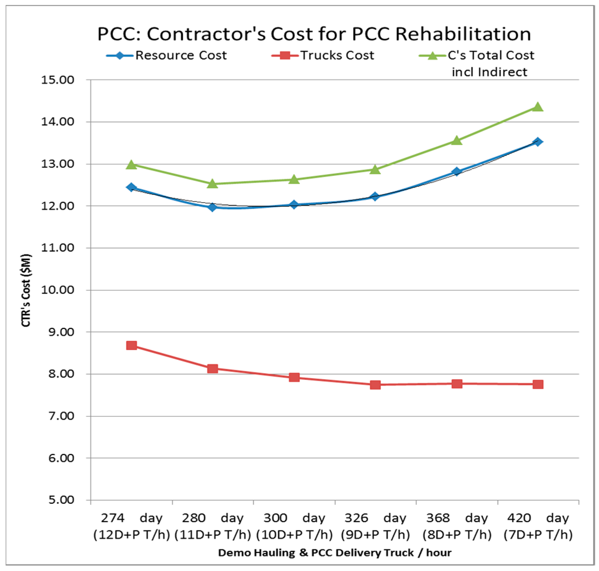
6.4. Contractor Acceleration Incorporated with Resource Mobilization

One of the major contributions of this process is the inclusion of contractor acceleration costs and savings the contractor may experience in accelerating the project. These values can be calculated using Equation (6) but, if more accuracy is desired, can also be calculated through the support of commercial cost estimating database software (such as the RS Means). Using RS Means and CA4PRS to calculate contractor acceleration is discussed in greater detail within this section. The above example used Equation (6), assuming the SHA was content with that level of accuracy. This results in a constant cost/day contractor acceleration charges and savings. However, for this example and often in construction, a contractor’s acceleration charges are much more complex.

The contractor reduces construction duration by increasing efforts (increasing number of crews or equipment and workers) for pavement reconstruction activities than they planned in the bid proposal. This resource/schedule relationship is important for SHAs to understand in developing their I/Ds and the CA4PRS schedule module can demonstrate the sensitivity of the contractor’s pavement crew size effect on the construction duration (total closure number). Several case studies in the western state DOTs (CA, WA, UT and etc.) in the course of CA4PRS validation studies indicated that the most critical contractor’s resource to control the pavement reconstruction productivity (i.e., daily progress) is their delivery and hauling trucks, therefore the CA4PRS focuses on these resources in its acceleration calculations.

For the above mentioned I-15 Ontario project, CA4PRS schedule analysis utilized the typical pavement reconstruction crew size of 10 hauling dump trucks per hour to remove the existing concrete pavement from the site to the dumping yard and 10 concrete dump trucks per hour to deliver the concrete from the batch plant to the site. With this typical truck resource size and the contractor’s other pavement reconstruction resources in the CA4PRS Schedule Analysis module, the results indicate that the normal duration of the construction closure is 300 days of 8-h nighttime closures, which is consistent with Equation (5). Changing the pavement hauling and delivery trucks from the “normal crew” size directly influences the closure duration. This can be seen in Figure 5 below with Trucks/hour ranging from 12 down to 7.

In adding trucks, the contractor incurs increased trucking charges but also receives decreased overhead costs resulting in savings (contractor savings included in Equation (7)). It would be logical to think that more trucks would always equate to reduced overhead costs. However, we see a drop in total costs from 12 to 11 trucks in Figure 5. This is likely due to the efficiencies loss of production/overhead in using 12 trucks. As the number of trucks decreases from 11 to 7, a drop in tuck charges can be seen but with a rapidly increasing total cost. This is due to the increased duration equated to less trucks and therefore greater contractor’s overhead charges. This illustration is simply used to show the non-linear nature of contractor acceleration costs/savings that SHAs should be aware of. Also depicted is how CA4PRS provides SHAs with the necessary tools to calculate said cost/savings and use in their I/D calculations.

7. Conclusions

The US FHWA has encouraged SHAs to implement I/D contracting provisions to reduce traffic disruption during highway construction, especially when lanes closure severely disrupts highway traffic, significantly increase RUC, or have a significant impact on adjacent neighborhoods or businesses [2]. However, effectively determining the optimum I/D value is difficult. This research has presented an eleven-step I/D development optimization process that is repeatable and auditable. It also includes an equation for calculating the incentive value based on contractor acceleration costs and incorporating RUC, agency costs and contractor acceleration savings. The tool also incorporates a FHWA promoted national tool to calculate work zone impacts and costs and Shr et al.’s [12] previously validated time-cost tradeoff I/D model, though these tools can be replaced by those used by the SHA.

The process in this paper represents a systematic, practical tool for optimizing I/D amounts. The process is an advancement of existing practice and literature as it has the capability to be used internationally across all SHAs with minimal modifications, especially on urban highway renewal projects for more efficient infrastructures sustainability. It also reducing the contractors’ ability to pursue unlawful penalty claims as it provides a detailed and auditable way to calculate disincentives based on actually incurred costs increasing the ability to defend its value in court. Finally, it is based on the contractors’ acceleration costs, providing a formula for calculating a reasonable contractor bonus (to incentivize acceleration) based on a sharing of agency acceleration savings, currently missing in literature.

In implementing the process through one California highway project, the author found the current SHA I/D practices to be lacking as they covered the contractor’s acceleration costs at best. As an incentive is meant to encourage acceleration, simply covering the contractor’s costs is insufficient for motivation. In contrast, the proposed process provided a clear and simple I/D calculation that incorporates both the contractor’s cost and a reasonable bonus. Although adding contractor bonus has been proposed in previous literature [11], the solution was vague and difficult for SHAs to implement.

8. Limitations and Recommendations for Future Research

The presented tool relies heavily on CA4PRS and Shr et al.’s [11] model and has been developed for US rehabilitation/reconstruction projects. While these are state-of-the-art tools, CA4PRS is only available for the US and Shr et al.’s model is currently a prototype. In replicating and improving Shr et al.’s methodology, the process within this paper can be modified for any area but will require a large SHA database of project performance and a statistician. Also, different models need to be made for different project types [29] which means a SHA may be required to develop multiple models. Finally, the Shr et al. [11] model does not work well when the RUC plus agency cost is relatively high or low compared to the contractor’s construction cost. With a high RUC plus agency cost, the total cost curve may never converge and the concept of the optimizing total cost may be difficult to apply. Alternatively, if the daily RUC and agency is relatively low compared to the contractor’s cost, the total cost curve can converge easily in a short period of time and then the maximum acceleration is short compared to the normal duration. It should be noted that SHAs can replace the CA4PRS and Shr et al.’s [11] model with more apt tools for the region and still benefit from the I/D process presented (still all-encompassing and based on contractor acceleration). Finally, the process can also be used for new construction with changes to the RUC calculation process (road users would not be impacted by work zones as it would be stand-alone, new construction).

Although this process provides a systematic way to calculate I/D values, it does not entirely remove the requirement of engineering judgement. While the process presents an adjusted I/D calculation (Equation (7)), with suggested guidelines on what values to use for project traffic volumes, the engineer still needs to use their judgement in the conversion and discount factors. To aid in this judgement, the CA4PRS program plus excel spreadsheet includes a “what-if” sensitivity analysis. This analysis allows the engineer to see the incentive, optimal acceleration and disincentives given different assumptions of the normal construction cost (engineer’s estimate), construction duration and discount factors. This process is in the prototype phase and is therefore not included in this paper but an example of its implementation was included in the Final FHWA report [20].

References

1. Mallela, J.; Sadavisam, S. Work Zone Road User Costs: Concepts and Applications; US Department of Transportation, Federal Highway Administration: Washington, DC, USA, 2011.
2. Federal Highway Administration (FHWA). Incentive/Disincentive for Early Contract Completion. In FHWA Technical Advisory T5080.10; Federal Highway Administration (FHWA): Washington, DC, USA, 1989. Available online: http://www.fhwa.dot.gov/construction/contracts/t508010.cfm (accessed on 3 March 2018).
3. Herbsman, Z.J.; Tong Chen, W.; Epstein, W.C. Time is money: Innovative contracting methods in highway construction. J. Constr. Eng. Manag. 1995, 121, 273–281. [Google Scholar] [CrossRef]
4. Sillars, D.N.; Leray, J.P.A. Incentive/Disincentive Contracting Practices for Transportation Projects; ASCE Press: Washington, DC, USA, 2006. [Google Scholar]
5. Sun, C.; Edara, P.; Mackley, A. Refocusing on Liquidated Damages in Incentive/Disincentive Contracts. J. Leg. Aff. Disput. Resolut. Eng. Constr. 2013, 5, 136–141. [Google Scholar] [CrossRef]
6. Fick, G.J. Time-Related Incentive and Disincentive Provisions in Highway Construction Contracts; Transportation Research Board: Washington, DC, USA, 2010; Volume 652.
7. Gillespie, J. Estimating Road User Costs as a Basis for Incentive/Disincentive Amounts in Highway Construction Contracts; Virginia Transportation Research Council: Charlottesville, VA, USA, 1998.
8. Jiang, Y.; Chen, H. The Effects of User Costs at Highway Work Zones on the Incentive and Disincentive Values of Highway Construction Projects. In Proceedings of the 18th CIB World Building Congress, Salford Quays, UK, 10–13 May 2010. [Google Scholar]
9. Yimin, Z.; Irtishad, A. Developing a Realistic-Prototyping RUC Evaluation Tool for FDOT; US Department of Transportation: Washington, DC, USA, 2008.
10. Shr, J.-F.; Chen, W.T. Setting maximum incentive for incentive/disincentive contracts for highway projects. J. Constr. Eng. Manag. 2004, 130, 84–93. [Google Scholar] [CrossRef]
11. Sillars, D.N. Establishing Guidelines for Incentive/Disincentive Contracting at ODOT; Oregon State Library: Salem, OR, USA, 2007.
12. Shr, J.-F.; Thompson, B.; Russell, J.; Ran, B.; Tserng, H. Determining minimum contract time for highway projects. Transp. Res. Rec. J. Transp. Res. Board 2000, 1712, 196–201. [Google Scholar] [CrossRef]
13. American Association of State Highway and Transportation Officials (AASHTO). Primer on Contracting for the Twenty-First Century; Report; Contract Administration Section of the AASHTO Subcommittee on Construction: Washington, DC, USA, 15 June 2006. [Google Scholar]
14. Ellis, R.D., Jr.; Pyeon, J.-H.; Herbsman, Z.J.; Minchin, E.; Molenaar, K. Evaluation of Alternative Contracting Techniques on FDOT Construction Projects; Department of Civil and Coastal Engineering, University of Florida: Gainesville, FL, USA, 2007. [Google Scholar]
15. Florida Department of Transportation (FDOT). Alternative Contracting Methods; Office of Inspector General Audit Report 04B-0001: Tallahassee, FL, USA, 2000.
16. Shr, J.F.; Chen, W.T. Functional Model of Cost and Time for Highway Construction Projects. J. Mar. Sci. Technol. 2006, 14, 127–138. [Google Scholar]
17. Cusack, M.M. Construction Management—The Way Forward, Investment, Procurement and Performance in Construction; E & FN Spon: London, UK, 1991. [Google Scholar]
18. Shen, L.; Drew, D.; Zhang, Z. Optimal bid model for price-time biparameter construction contracts. J. Constr. Eng. Manag. 1999, 125, 204–209. [Google Scholar] [CrossRef]
19. Pyeon, J.H.; Lee, E.B. Systematic Procedures to Determine Incentive/Disincentive Dollar Amounts for Highway Transportation Construction Projects; Mineta Transportation Institute Research Report 11-22; SJSU Research Foundation: San Jose, CA, USA, June 2012. [Google Scholar]
20. Federal Highway Administration. Quantification of Cost, Benefits and Risk Associated with Alternative Contracting Methods and Accelerated Performance Specifications. Federal Highway Administration Project, Contract No. DTFH61-11-D-00009, 2013–2016. Available online: https://www.fbo.gov/index?s=opportunity&mode=form&id=a4c450b35ead6e702cd29cf108be1826&tab=core&_cview=1 (accessed on 3 March 2018).
21. Collura, J.; Heaslip, K.; Knodler, M.; Ni, D.; Louisell, W.C.; Berthaume, A.; Khanta, R.; Moriarty, K.; Wu, F. Evaluation and Implementation of Traffic Simulation Models for Work Zones. 2010. Available online: http://www.ct.gov/dot/LIB/dot/documents/dresearch/NETCR80_05-8.pdf (accessed on 3 March 2018).
22. Lee, E.B.; Ibbs, C.W. A Computer Simulation Model: Construction Analysis for Highway Rehabilitation Strategies (CA4PRS). JCEM 2005, 131, 449–458. [Google Scholar]
23. Federal Highway Administration (FHWA). Construction Analysis for Pavement Rehabilitation Strategies (CA4PRS). Available online: https://www.fhwa.dot.gov/research/deployment/ca4prs.cfm (accessed on 8 March 2017).
24. Transportation Research Board, National Research Counsel. Highway Capacity Manual (HCM) 2000; Transportation Research Board, National Research Counsel: Washington, DC, USA, 2000.
25. Lee, E.-B.; Thomas, D.K.; Bloomberg, L. Planning urban-highway reconstruction with traffic demand affected by construction schedule. J. Transp. Eng. 2005, 11, 752–761. [Google Scholar] [CrossRef]
26. Taylor, T.R.; Brockman, M.; Zhai, D.; Goodrum, P.M.; Sturgill, R. Accuracy analysis of selected tools for estimating contract time on highway construction projects. In Proceedings of the Construction Research Congress 2012: Construction Challenges in a Flat World, West Lafayette, IN, USA, 21–23 May 2012; pp. 217–225. [Google Scholar]
27. Fekpe, E.; Gopalakrishna, D.; Middleton, D. Highway Performance Monitoring System Traffic Data for High-Volume Routes: Best Practices and Guidelines; Federal Highway Administration: Washington, DC, USA, 2004.
28. California Department of Transportation (Caltrans). Memorandum: Delegation of Authority for Use of A + B Bidding and Incentive/Disincentive Provisions. Available online: http://www.dot.ca.gov/hq/oppd/design/m061200.pdf (accessed on 12 March 2017).
29. Shuka, A. An Exploration of the Relationship between Construction Cost and Duration in Highway Projects. Master’s Thesis, University of Colorado at Boulder, Boulder, CO, USA, 1 January 2017. [Google Scholar]
Figure 1. I/D Time-Cost Tradeoff (modified from Shr et al. [12]).
Sustainability 10 00701 g001
Figure 2. Research Methodology.
Sustainability 10 00701 g002
Figure 3. Steps in I/D Optimization Assessment Process.
Sustainability 10 00701 g003
Figure 4. I-15 Ontario Time-Cost Trade-off Curve Graph.
Sustainability 10 00701 g004
Figure 5. Graphic Representation of Contractor’s Resource Sensitivity.
Sustainability 10 00701 g005