Spatial Assessment of Urban Flood Susceptibility Using Data Mining and Geographic Information System (GIS) Tools


1
Center for Environmental Assessment Monitoring, Environmental Assessment Group, Korea Environment Institute (KEI), 370 Sicheong-Daero, Sejong 30147, Korea
2
Department of Geoinformatics, University of Seoul, 163 Seoulsiripdaero, Dongdaemun-gu, Seoul 02504, Korea
3
Geological Research Division, Korea Institute of Geoscience and Mineral Resources (KIGAM), 124 Gwahak-ro, Yuseong-gu, Daejeon 34132, Korea
4
Geophysical Exploration, Korea University of Science and Technology, 217 Gajeong-ro, Yuseong-gu, Daejeon 34113, Korea
*
Authors to whom correspondence should be addressed.
Sustainability 2018, 10(3), 648; https://doi.org/10.3390/su10030648
Submission received: 2 January 2018
/
Revised: 12 February 2018
/
Accepted: 15 February 2018
/
Published: 28 February 2018
(This article belongs to the Special Issue Floods and Landslides: A Sustainability Approach)
Abstract
:Using geographic information system (GIS) tools and data-mining models, this study analyzed the relationships between flood areas and correlated hydrological factors to map the regional flood susceptibility of the Seoul metropolitan area in South Korea. We created a spatial database of data describing factors including topography, geology, soil, and land use. We used 2010 flood data for training and 2011 data for model validation. Frequency ratio (FR) and logistic regression (LR) models were applied to 2010 flood data to determine the relationships between the flooded area and its causal factors and to derive flood-susceptibility maps, which were substantiated using the area flooded in 2011 (not used for training). As a result of the accuracy validation, FR and LR model results were shown to have 79.61% and 79.05% accuracy, respectively. In terms of sustainability, floods affect water health as well as causing economic and social damage. These maps will provide useful information to decision makers for the implementation of flood-mitigation policies in priority areas in urban sustainable development and for flood prevention and management. In addition to this study, further analysis including data on economic and social activities, proximity to nature, and data on population and building density, will make it possible to improve sustainability.
1. Introduction
The increase in global temperatures, seasonal shifts, and precipitation increases are just a few of the many consequences of climate change that are currently experienced on a daily basis [1,2]. Heavy rains, typhoons, floods, and other meteorological conditions cause variation in the hydrological system and increase the pressure on drainage systems, waterworks, and sewerage facilities in urban areas [3,4]. In addition, an increase in impermeable surfaces such as buildings and roads can lead to an exponential increase in surface flow by decreasing the absorption and storage of rainwater below the surface [3]. Subsequently, with a higher concentration of rainwater in rivers, flooding risks increase substantially. Therefore, it is vital to assess and prevent these risks in urban areas to promote sustainability. Countermeasures to prevent urban flooding such as the extension of drainage pipelines and the improvement of undercurrent facilities and pumping stations are vital; they require that information on susceptible areas be obtained prior to flooding. Hence, flood susceptibility assessment is required for decision making and prioritization in order to minimize flood damage.
Recent advances in technology, including the spread of the Internet and mobile devices, has led to an exponential increase in the accumulation of data, whilst the development of hardware and distributed-parallel processing technology has improved our ability to accumulate data, providing the basis for data mining [5]. In order to increase the utilization of large databases, it is important to make reasonable and rapid decisions, and to find significant information that can support decision making [6]. In this environment, modeling is evolving with data-based learning instead of laboratory-based learning. Data-mining techniques are useful in elucidating the mechanisms between certain events and related variables [7]. In this paper, data mining is performed to analyze the correlation between flood data and related factors used in previous research.
The Seoul metropolitan area, the capital and largest city of the Republic of Korea, suffers from extensive flood damage attributable to heavy rainfall during the summer. Flood susceptibility maps are essential to prevent and skillfully manage flood disasters. In this study, we generated flood susceptibility maps for the Seoul metropolitan area using data-mining models in a geographic information system (GIS) environment. Many studies have applied GIS and remote-sensing techniques to produce thematic maps related to geomorphology, land cover, drainage patterns, geology, and soils [8,9,10].
Due to a complex set of flood-related factors, it is important to use data-mining techniques to make a suitable assessment of flood susceptibility. Various data-mining approaches have been used for decades to predict and assess flood occurrence [11,12]. In general, soft computing or statistical data-mining techniques have recently been used, such as the decision-tree based model [13,14,15], artificial neural network (ANN) based model [16,17,18], support-vector machine [19,20,21] or the logistic regression (LR) model [22,23]. Proactively, a basic statistical model, frequency ratio (FR), is used to observe trends between flood-related factors and flood events [24,25,26,27]. More in-depth assessments have incorporated numerical modeling and analytic hierarchy process analysis [28,29,30] Some studies have demonstrated hydraulic models or created additional thematic maps by mixing geophysical surveys with GIS [31,32,33] and remote-sensing techniques [34,35]. In this study, flood susceptibility analysis was performed by using FR and LR models, which are the most basic statistical data-mining models, for the case study in the Seoul metropolitan area.
Individual efforts to predict floods related to climate change and to design measures to efficiently prevent flooding include studies of climate change, the correlation of rainfall and flooding, and statistical analysis methodology for floods [36,37,38,39,40,41,42]. Studies mapping flood hazards [43,44,45] and analyzing the effects of urban growth or other factors on flooding [46,47] have been conducted. The purpose of this study is to map the regional flood susceptibility of the Seoul metropolitan area in South Korea by using the data-mining and GIS techniques. Therefore, in the current study, we contributed to this body of work by generating susceptibility maps based on FR and LR models as a case study in this study area. These models were then validated to assess the sensitivity of the Seoul metropolitan area to floods.
2. Study Area
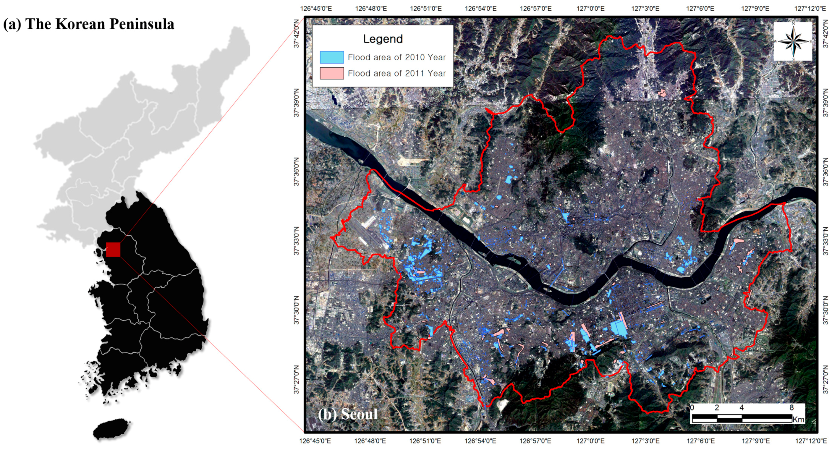
Seoul is located in the middle of the Korean peninsula, covering an area of 605.41 km2 at 126°59′40″ E, 37°33′59″ N (Figure 1). Although the city accounts for less than 1% of the total area of South Korea, 2011 census statistics indicated that the population had reached approximately 10 million citizens or approximately one-quarter of the total population of South Korea. Due to the high frequency of temporary population migration, the city has a highly developed traffic system, which is vulnerable to serious damage during natural disasters such as landslides [1].
Seoul has a coastal climate, with an average annual temperature (1981–2010) of 12.5 °C. Although the cold high-pressure system of the continent affects the city in winter, the influence of the Sea of Okhotsk in summer typically leads to a seasonal temperature difference of 30 °C. The average annual precipitation is 1450 mm, and most precipitation occurs during the summer. The city is situated in a natural basin surrounded by numerous peaks over 300 m a.s.l. The highest peaks are Bukhansan (836 m), Dobongsan (740 m), Inwangsan (338 m), and Gwanaksan (629 m). Historically, these mountains have served as a natural fortress, protecting the city from damage. Other important mountains in the region are Buaksan (342 m), which protects the presidential palaces of Cheongwadae and Namsan (232 m), the old city shield of Seoul. The city is divided into Gangbuk and Gangnam, on the Han River, which is one of four major rivers in Korea. Gangbuk developed in the valley between Dobongsan and Bukhansan. The region where the Cheonggyecheon, Jungnangcheon, and Han Rivers join is an alluvial plain. Geologically, the bedrock of Seoul is mainly granite and gneiss, which greatly affects the topography and soil. In the western part of the Gangbuk area, there are mainly banded gneisses; the eastern part contains mainly Daebo granite. In the Gangnam region, banded gneiss is present in the east, whereas a mixture of Daebo granite or granite gneiss and schist dominate in the west (Figure 2).
3. Spatial Datasets
Flood susceptibility is commonly determined using a number of factors such as hydrological factors, topographical characteristics such as surface and slope types, rivers, meteorological factors, soil and vegetation characteristics, and land-use or development status. In this study, we selected the 11 hydrological factors expected to be related to flood susceptibility and applied these to FR and LR models (Table 1, Figure 3). We identified areas experiencing frequent floods and, using an administrative area-based survey, generated an inventory map containing 4338 flooded zones within the entire area. Different sample sizes have been suggested in the literature for this type of analysis [48]. The flood-related factors considered in this study were collected and extracted from thematic maps provided by the South Korean government. The input data used in this study were factors related to topography, geology, land use, forests, and soil (Table 1).
Topography plays an extensive role in hydrogeological systems [49]. We created a digital elevation model (DEM) by applying the triangulated irregular network (TIN) method to contours digitized from a topographical map. The TIN was converted into a raster at a resolution of 5 × 5 m after removing the sink area, or internal drainage, from the elevation grid. Following the calculation of the DEM, the slope gradient was calculated from the DEM using the ArcGIS 10.0 software. The topographic wetness index (TWI), stream power index (SPI), and slope length factor (SLF) were also calculated from the DEM using the ArcView software (Version 10.1, Esri, Redlands, CA, USA). We extracted topographical factors because flood occurrence is influenced by the geomorphological characteristics of the region. Topography is an important element in the spatial variation in hydrological conditions [50]. We calculated the distance from the river using topographic maps. The SPI, an index of the erosive power of a stream, can be used to describe potential stream erosion at a given point on the surface of the terrain. As the area and slope of the watershed increase, the amount of water contributed to the upward slope and the water flow rate increase, causing an increase in the SPI value. The SPI index can be defined [40] as:
where As is the specific catchment area and b is the local slope gradient in degrees. TWI is a topographic factor used in the run-off model [51], and is defined as
where α is the bottom-up cumulative area accumulated through a point (per unit contour length) and b is the slope angle at that point. TWI, the lateral transmission coefficient on the ground surface, indicates the probability of water flowing to a specific point on a local slope [51]. The TWI index reflects the accumulation trend of water at any point in the watershed in terms of α and reflects the tendency of gravity to move the water along a slope, with tanβ representing the approximate hydraulic gradient. Water infiltration depends mainly on the permeability and other properties of the material such as pore pressure, which affects soil strength [52]. The SLF for average erosion given a slope length λ, which is in feet (i.e., imperial units), varies as:
where 72.6 is the revised universal soil-loss equation unit plot length in feet and m is a variable slope–length exponent [52]. The slope–length index β is the ratio of rill to inter-rill erosion due to raindrop impact and rill erosion caused by flow, as shown in the following equation [53]:
where
where θ is slope steepness angle. From the land-use map, the type of impermeable land use, agricultural land use and retarding basin factors were extracted. We classified the regions into six types of impermeable land-use areas: residential, manufacturing, commercial, recreational, traffic, and public. In addition, soil-drainage and geology data were derived from soil map and geological map, respectively.
Thematic maps that include flood-related factors were acquired in vector format using the ArcGIS package. The 11 related factors (Table 1) calculated or extracted during this procedure were resampled to raster data at a 10 m spatial resolution and converted into a GRID file. We constructed a spatial database with a total of 11,222,445 cells (3705 rows × 3029 columns). There were a total of 127,087 flooded cells for 2010 and 65,964 for 2011. All of the factors were converted into ASCII format to apply the LR model. Before calculating the frequency ratios of the types and categories of each factor, the factors were classified into 10 equal-area classes. The 10 classes were automatically determined by stipulating a similar number of cells in the total area.
4. Method
Effective decision making requires both data and predictions based on potential conditions. Therefore, we applied the principle of conditional probability and selected an FR model to determine the spatial relationship between flooded areas and flood-related factors. We subdivided the data layer into classes within each study area, based on the percentage of the total area that was flooded [54]. In Equation (6), P(P) represents the area ratio of a class or type to a given number of unit cells, including the domain fraction of the class; P(O) is the percentage of flood occurrence within the class [55]. Then the FR value of the type or class of each factor C is:
We determined the correlations between flood-related factors using the FR model. A high correlation with flooding was represented by a value greater than 1 and low correlation by a value less than 1. Then we used these correlations to generate flood-susceptibility maps. Using the GIS, we reclassified all of the ratios composed of raster types to 10 classes on the basis of equivalent areas and calculated the FR for each class or type of each factor [56]. Finally, we determined flood susceptibility using the FR model, adding all of the factors using raster calculation functions in the GIS to merge the factors. The LR model is a multivariate analyses model useful for making predictions based on input variables. The purpose of LR is to explain the relationship between the dependent and independent variables [57]. In this study, the input into the LR model included observed values and the presence/absence of predictive variables, indicated by binary numbers. The dependent variable of the LR model was a categorical or binary number. An advantage of the LR model is that the independent variables can be either continuous or categorical, and additional link functions can be added to a general linear regression model to allow for continuous, discrete, or a combination of variable types. In this study, the dependent variable was the location of the flood and the independent variables were flood-related factors. We used the SPSS 21 statistical package to calculate the coefficients for each factor in the LR model [58]. The relationship between flood occurrence and the input factors can be conceptualized as:
where Λ is the logistic function. Then, the LR model is:
where P is the estimated probability of the event, or susceptibility to flooding based on intrinsic properties [59]. The resulting curve is S-shaped, whereas z represents a linear combination. Therefore, the LR model implies that the data matches the following equation:
where bi (i = 1, 2, …, n) values are the slope coefficients for the LR model and xi (i = 1, 2, …, n) values are the independent variables [49]. The extracted linear model becomes an LR depending on the presence/absence of a flood given the values of the independent variables that were related to flood occurrence in previous years. Figure 4 shows a flowchart outlining the methodology used in this study. Areas flooded in 2010 and 2011 were used to demonstrate the application and validity of the resulting flood-susceptibility maps (Figure 1 and Figure 2). Areas flooded in 2010 were used as dependent variables and the hydrological factors were used as independent variables. The spatial database determined that a total of 11 topography factors including soil, geology and land-use data were appropriate independent variables for the model. Therefore, calculated or extracted factors and the 2010 flooded areas were included in the LR model. To compare the results of the LR model with those of the probabilistic model, we applied an FR model in the flood-susceptibility analysis. The SPSS 20 statistical package was used in combination with GIS software to run these models. We validated the susceptibility map for the study area using areas flooded in 2011. To calculate the LR coefficients for the flood-related factors, we converted the spatial database to ASCII files using ArcGIS 10.0 and SPSS 20. The z values were multiplied by the coefficients and retrieved by adding the variables to these acquired coefficients in the GIS environment. We created flood-susceptibility maps by gathering flood-related data from topographic, geological, soil, and land-use maps, and constructing a spatial database describing the areas flooded in 2010. The database was established in a grid format and flood-susceptibility assessment was performed using the LR and FR models. After the study area was selected, we isolated the flooded areas for 2010 and 2011. The 2010 flooded area was used for training and the 2011 flooded area was used for validation.
z = b0 × 0 + b1 × 1 + b2 × 2 + … + bn × n
5. Result
5.1. Relationships between Flooded Area and Related Factors
The results of the FR model showed the relationship between the input factors from the geospatial database and the flooded area data used for training. Flooding was shown to occur at low altitudes and in regions with gentle slopes. In this study, topographical factors calculated from the DEMs were strongly correlated with flood susceptibility (Table 2), which indicates high flood susceptibility in these regions. The water flow traveled downslope from regions with high potential, where water is recharged, to those with low potential. Slope was an important factor influencing the balance between infiltration and runoff. The FR of slope under 8.58 degrees showed over 1.0, which is relatively higher than FR values of higher slope (<1.0). Penetration was inversely proportional to the slope, and there was more infiltration and less runoff in regions with gentle slopes [60]. FR of SLF shows a similar trend with that of slope gradient. As a result, the rainfall runoff rate increased, the infiltration rate decreased, and flood susceptibility decreased where elevation was high and slope was steep. Conversely, low elevation and gentle slope produced the opposite results. A higher TWI value indicates a larger area of lower slope; therefore, the higher the TWI, the greater the susceptibility to floods. There was a positive correlation between TWI and flood occurrence and a negative correlation between distance from the river and flood occurrence. This implies that flood susceptibility decreases with distance from the river.
For the impermeable land-use areas, the frequency ratio was higher in residential and traffic areas and lower in manufacturing and recreational areas. The FR of non-green farm area (1.11) and barren ground (0.78) showed relatively higher value followed by field (0.39) and paddy (0.33) areas. In the retarding basin area, the relationship with flood occurrence is very low, with a FR value of 0.27. FR values were higher in poorly, somewhat poorly, and moderately well-drained soil areas (>1.0), and lower in well-drained soils (Table 2). Among the seven geological unit classes (porphyroblastic gneiss, limestone, alluvium, schist, garnet-bearing granite gneiss, banded gneiss, granitoid, and granite gneiss), the FR values were higher for alluvium (2.03), garnet-bearing granite gneiss (1.82), schist (1.79). Schist and banded gneiss showed lower FR values (<1.0), while others (pophyroblastic gneiss, granitoid granite gneiss) showed zero. Overall, FR results showed a correlation between flood occurrence and each factor.
5.2. Flood Susceptibility Mapping and Its Validation
The FR model was used to derive the correlation between flood occurrence area and flood-related factors in the previous step. A grade for each element was defined as a category or range according to the type of each factor, and the ratio of non-flooded area to flooded area is shown in Table 2. We obtained an FR map for each factor by spatially replacing the FR value for each class. Finally, the flood susceptibility map was obtained by summing all FR maps for each factor, as:
FR = ∑Fr (Fr, Rating of each factors’ type or range)
We analyzed the relationship between flooded area and total area, and generated a flood susceptibility map using an LR model for further analysis (Figure 5). The LR coefficients (B), standard error of the slope coefficient (SE), and significance level (Sig.) of the variables were estimated using the maximum likelihood model (Table 3). An iterative algorithm is essential for parameter estimation in logistic multiple regression models when the relationship between independent variables and probabilities is non-linear [61]. DEM, TWI, distance from the river, type of impermeable land use, type of agricultural land use, detention basin, soil drainage, and geology were important factors (P < 0.05). However, these results cannot be considered definitive [62]. Therefore, we used 11 factors to predict flooding for management purposes. The Hosmer and Lemeshow ‘goodness-of-fit’ test resulted in a value less than 0.05 [63]; thus, the LR model was suitable for predicting flood susceptibility. We multiplied continuous data such as DEM, slope, SLF, SPI and TWI by the coefficients obtained. Factors expressed by categorical data were multiplied by coefficients obtained for each class (Table 2). Then we spatially summed all of the layers and added Z, a forecast parameter. Probabilities were calculated for all factors and the flood susceptibility was mapped using the LR coefficients (Equation (11), Table 3). As a result of the analysis, TWI in the topographic factors, distance from the river, residential area, commercial area, trafficked area and public area in terms of land use showed positive value of higher effects. Retarding basin, soil drainage and geology factors also showed positive values in all classes except for limestone.
Z = (−0.007 × DEM) + (−0.005 × SLOPE) + (−0.006 × SLF) + (−0.025 × SPI) + (0.20 × TWI) + DISTANCE FROM THE RIVER + TYPE OF IMPERMEABLE LAND USE + TYPE OF AGRICULTURAL LAND USE + RETARDING BASIN + SOIL DRAINAGE + GEOLOGY − 21.853
Continuous data such as DEM, slope, SLF, SPI and TWI values are multiplied by the coefficient obtained. The other factors of categorical data were also multiplied by the coefficients obtained for each class in Table 2. Lastly, all the layers are spatially summed and Z, a forecast parameter, is added. The probability of factors was calculated and the flood susceptibility was mapped by using the LR coefficients in Table 3 and Equation (11).
According to the results, flood susceptibility is high in low-lying areas near the river which is affected by the distance from the river factor. In particular, the susceptibility of floods was high in the southern part of the river, and as the distance from the river increases, the occurrence of floods decreases. There are places where the park facilities show a somewhat high susceptibility near the Han River, which is the main river of the city. Also, the spatial pattern shows that banded gneiss and schist wield a great influence upon the high-susceptibility area.
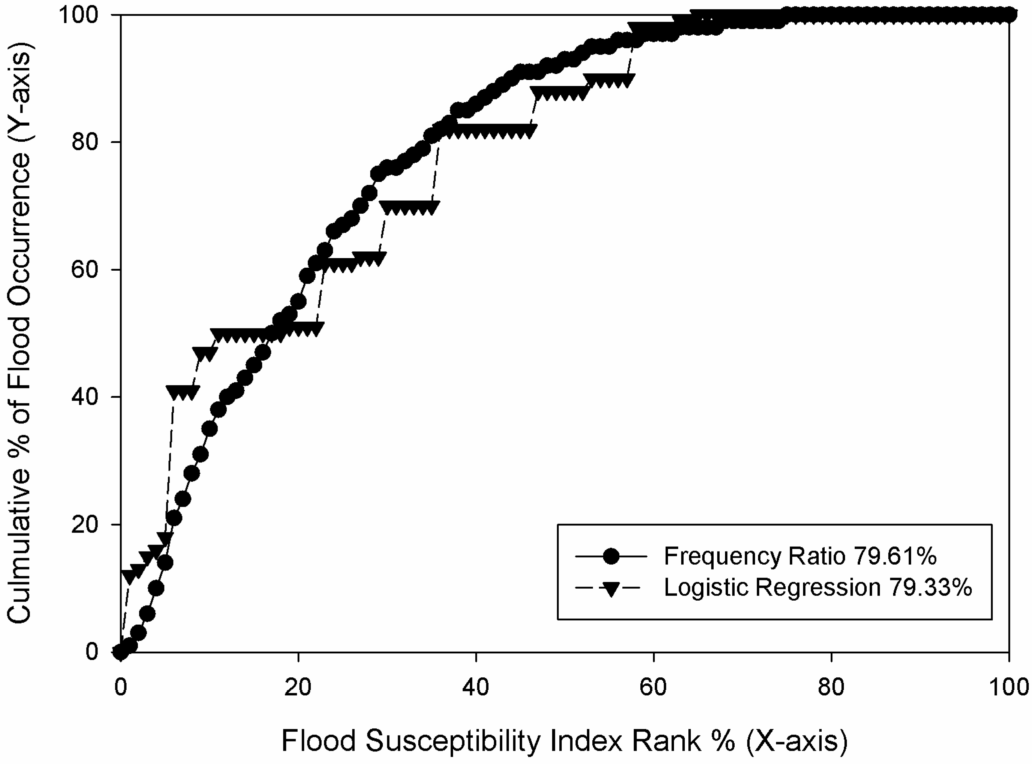
In this study, FR and LR models were applied using data from extensive flooding in 2010. The flood susceptibility maps generated by these models should be used to predict areas where future floods might occur; therefore, we validated the models using data from 2011, the year after the flood used to train the models. We calculated the area under the curve (AUC) to create a ratio curve to qualitatively assess the accuracy of the flood-prediction maps’ area. In detail, to obtain relative ranks for the predicted patterns of the models, we sorted the susceptibility values of all cells in the study area in descending order, forming 100 classes accumulated in 1% intervals. For example, the LR model accounted for 33% of the flooded area and 10% of the total area. To quantitatively evaluate accuracy, we calculated the AUC assuming the entire study area to be 1.0. The AUC for the FR result was 0.7961 (i.e., the prediction accuracy was 79.61%). The accuracy of the LR model was 79.33% (Figure 6).
6. Discussion and Conclusions
Floods are among the most damaging hydrological natural disasters worldwide. Governments and research institutes have evaluated flood susceptibility at the national scale and conducted studies to predict the spatial distribution of flood events. In the current study, FR and LR models were applied to create flood susceptibility maps of the Seoul metropolitan area. In the preliminary step of this process, we selected 11 core variables affecting flood susceptibility, and constructed FR and LR models to determine the relationships between flooded areas with specific capacity and flood-related variables. Factors related to flood occurrence were collected in a spatial database and flood-susceptibility values for the study area were calculated. We validated the susceptibility-prediction results using data collected in previously flooded areas in years not used to train the models.
The FR model results showed that slope factors had a negative spatial relationship with flooded area, whereas TWI showed a positive correlation. Residential and transportation network areas were more susceptible to flooding than other land-use types, and schist units and moderately well-drained soil classes had a higher susceptibility than other related classes.
We compared and analyzed flood-susceptibility maps produced by the LR and FR models, and found that the accuracy of the LR model was 79.33% and that of the FR model was 79.61%. All of the results from both models demonstrated reliable results of over 75% accuracy.
Time-series analyses of floods are limited in that it is almost impossible to obtain data measuring the change in flood area over time; it needs to be performed by evaluating drainage capacity which affects flood occurrence in certain areas. In addition, existing location information related to flood damage is created based on interviews in the damaged areas, rather than using accurate coordinates; this method could create problems in the spatial analysis. During flooding, the handling capacity of the study site, which is affected by factors such as drainage systems, waterworks and sewer facilities, also plays an important role. However, it is difficult to acquire such data.
GIS and remote-sensing technologies enable the integration of different data sources and support decision-making through classified remote-sensing data [64]. GIS also allows quantitative assessment of changes over a wide range of spatial and temporal scales. Urban flood susceptibility was analyzed based on data-based learning with topographic, land-use, soil, and geological data in this case study. The validation results indicate that each factor used in this study is statistically significant. Several indicators related to flood susceptibility play an important role in water management, whose interdisciplinary nature requires a database designed to support decision-making in flood-susceptible areas containing diverse thematic information.
However, in this paper, the sewer system was assumed to have no influence. Although the city sewage system plays a very important role in flood occurrence, the underground materials in Seoul were classified as national institutional facilities which are treated as confidential. Also, the economic part such as land price or building information was not considered, since the land-price data in the present study area was not constructed very precisely. The urban infrastructure data such as building information is still partly constructed as spatial information on GIS, and the construction data has not been verified. Indeed, recent rainfall patterns are changing very intensively and it is very difficult to acquire the data that reflects the rainfall effect and complexity of urban areas such as the sewage system of the city. Based on the results of this study, further studies that reflect the sewer network would be possible, since all existing data are constructed as spatial information data, if only the sewer-related data is secured; also, the additional data could be used to enable economic analysis.
In this study, a limitation exists in validation due to the lack of field-observation data due to the property of a flood, which varies over time; and no separate correction for rainfall and flood occurrence were performed. The suggestion of this study is that the methodology of urban flood-susceptibility mapping will be used as a basis for establishing urban disaster-prevention policy and will contribute to protecting the public from flood disasters. The method applied in this study could also be used to map flood susceptibility in other regions in order to reduce flood risks to people and facilities, and to guide new infrastructure for the sustainable development of urban areas. The development of multiple models incorporating more case studies would permit future studies to generalize results based on flood-related factors.
Acknowledgments
This research was conducted at the Korea Environment Institute (KEI) with the support of “Climate Change Correspondence Program (2014001310006)” funded by the Korea Ministry of Environment (MOE) for Moung-Jin Lee. This research was supported by the Basic Research Project of the Korea Institute of Geoscience and Mineral Resources (KIGAM) funded by the Minister of Science, ICT and Future Planning of Korea for Saro Lee. This work was supported by the 2017 Research Fund of the University of Seoul for Hyung-Sup Jung.
Author Contributions
Sunmin Lee interpreted the results and wrote the paper. Hyung-Sup Jung designed the experiments and organized the paperwork. Moung-Jin Lee suggested the idea and applied the FR and LR models. Saro Lee collected data and conducted pre-processing of the input data. All the authors contributed to the writing of each section.
Conflicts of Interest
The authors declare no conflict of interest.
References
- Pachauri, R.K.; Allen, M.R.; Barros, V.R.; Broome, J.; Cramer, W.; Christ, R.; Church, J.A.; Clarke, L.; Dahe, Q.; Dasgupta, P. Climate Change 2014: Synthesis Report. Contribution of Working Groups I, II and III to the Fifth Assessment Report of the Intergovernmental Panel on Climate Change; IPCC: Geneva, Switzerland, 2014. [Google Scholar]
- Solomon, S. Climate Change 2007: The Physical Science Basis: Working Group I Contribution to the Fourth Assessment Report of the IPCC; Cambridge University Press: Cambridge, UK, 2007; Volume 4. [Google Scholar]
- Muneerudeen, A. Urban and Landscape Design Strategies for Flood Resilience in Chennai City; Qatar University: Doha, Qatar, 2017. [Google Scholar]
- Murray, V.; Ebi, K.L. IPCC Special Report on Managing the Risks of Extreme Events and Disasters to Advance Climate Change Adaptation (SREX); BMJ Publishing Group Ltd.: London, UK, 2012. [Google Scholar]
- Fayyad, U.; Piatetsky-Shapiro, G.; Smyth, P. From Data Mining to Knowledge Discovery in Databases; AI Magazine: California, USA, 1996; Volume 17, p. 37. [Google Scholar]
- Aronson, J.E.; Liang, T.P.; Turban, E. Decision Support Systems and Intelligent Systems; Pearson Prentice-Hall: Upper Saddle River, New Jersey, NJ, USA, 2005. [Google Scholar]
- Lee, S.; Lee, M.J.; Jung, H.S. Data mining approaches for landslide susceptibility mapping in Umyeonsan, Seoul, South Korea. Appl. Sci. 2017, 7, 683. [Google Scholar] [CrossRef]
- Diakakis, M.A. Method for flood hazard mapping based on basin morphometry: Application in two catchments in Greece. Nat. Hazards 2011, 56, 803–814. [Google Scholar] [CrossRef]
- Hardmeyer, K.; Spencer, M.A. Using risk-based analysis and geographic information systems to assess flooding problems in an urban watershed in Rhode Island. Environ. Manag. 2007, 39, 563–574. [Google Scholar] [CrossRef] [PubMed]
- Morelli, S.; Segoni, S.; Manzo, G.; Ermini, L.; Catani, F. Urban planning, flood risk and public policy: The case of the Arno River, Firenze, Italy. Appl. Geogr. 2012, 34, 205–218. [Google Scholar] [CrossRef]
- Harun, N.A.; Makhtar, M.; Aziz, A.A.; Zakaria, Z.A.; Abdullah, F.S.; Jusoh, J.A. The application of apriori algorithm in predicting flood areas. Int. J. Adv. Sci. Eng. Inf. Technol. 2017, 7, 763–769. [Google Scholar] [CrossRef]
- Mojaddadi, H.; Pradhan, B.; Nampak, H.; Ahmad, N.; Ghazali, A.H.B. Ensemble machine-learning-based geospatial approach for flood risk assessment using multi-sensor remote-sensing data and GIS. Geomat. Nat. Hazards Risk 2017, 8, 1080–1102. [Google Scholar] [CrossRef]
- Chapi, K.; Singh, V.P.; Shirzadi, A.; Shahabi, H.; Bui, D.T.; Pham, B.T.; Khosravi, K. A novel hybrid artificial intelligence approach for flood susceptibility assessment. Environ. Model. Softw. 2017, 95, 229–245. [Google Scholar] [CrossRef]
- Lee, S.; Kim, J.C.; Jung, H.S.; Lee, M.J.; Lee, S. Spatial prediction of flood susceptibility using random-forest and boosted-tree models in Seoul metropolitan city, Korea. Geomat. Nat. Hazards Risk 2017, 8, 1185–1203. [Google Scholar] [CrossRef]
- Rahmati, O.; Pourghasemi, H.R. Identification of critical flood prone areas in data-scarce and ungauged regions: A comparison of three data mining models. Water Resour. Manag. 2017, 31, 1473–1487. [Google Scholar] [CrossRef]
- Aziz, K.; Rahman, A.; Fang, G.; Shrestha, S. Application of artificial neural networks in regional flood frequency analysis: A case study for Australia. Stoch. Environ. Res. Risk Assess. 2014, 28, 541–554. [Google Scholar] [CrossRef]
- Elsafi, S.H. Artificial neural networks (ANNs) for flood forecasting at Dongola Station in the River Nile, Sudan. Alex. Eng. J. 2014, 53, 655–662. [Google Scholar] [CrossRef]
- Kasiviswanathan, K.S.; Sudheer, K.P. Comparison of methods used for quantifying prediction interval in artificial neural network hydrologic models. Model. Earth Syst. Environ. 2016, 2, 22. [Google Scholar] [CrossRef]
- Ahmadi, M.A.; Pournik, M.A. Predictive model of chemical flooding for enhanced oil recovery purposes: Application of least square support vector machine. Petroleum 2016, 2, 177–182. [Google Scholar] [CrossRef]
- Shi, Y.; Cheng, T.; Taalab, K. Flood Prediction Using Support Vector Machines (SVM). In Proceedings of the 24th GIS Research UK (GISRUK) Conference, London, UK, 30 March–1 April 2016; University of Greenwich: London, UK, 2016. [Google Scholar]
- Tehrany, M.S.; Pradhan, B.; Mansor, S.; Ahmad, N. Flood susceptibility assessment using GIS-based support vector machine model with different kernel types. Catena 2015, 125, 91–101. [Google Scholar] [CrossRef]
- Ettinger, S.; Mounaud, L.; Magill, C.; Yao-Lafourcade, A.F.; Thouret, J.C.; Manville, V.; Negulescu, C.; Zuccaro, G.; De Gregorio, D.; Nardone, S. Building vulnerability to hydro-geomorphic hazards: Estimating damage probability from qualitative vulnerability assessment using logistic regression. J. Hydrol. 2016, 541, 563–581. [Google Scholar] [CrossRef]
- Lee, S.; Lee, M.J. Susceptibility mapping of Umyeonsan using logistic regression (LR) model and post-validation through field investigation. Korean J. Remote Sens. 2017, 33, 1047–1060. [Google Scholar]
- Bathrellos, G.; Karymbalis, E.; Skilodimou, H.; Gaki-Papanastassiou, K.; Baltas, E. Urban flood hazard assessment in the basin of Athens metropolitan city, Greece. Environ. Earth Sci. 2016, 75, 319. [Google Scholar] [CrossRef]
- Khosravi, K.; Nohani, E.; Maroufinia, E.; Pourghasemi, H.R. A GIS-based flood susceptibility assessment and its mapping in Iran: A comparison between frequency ratio and weights-of-evidence bivariate statistical models with multi-criteria decision-making technique. Nat. Hazards 2016, 83, 947–987. [Google Scholar] [CrossRef]
- Rahmati, O.; Pourghasemi, H.R.; Zeinivand, H. Flood susceptibility mapping using frequency ratio and weights-of-evidence models in the Golastan Province, Iran. Geocarto Int. 2016, 31, 42–70. [Google Scholar] [CrossRef]
- Tehrany, M.S.; Pradhan, B.; Jebur, M.N. Flood susceptibility analysis and its verification using a novel ensemble support vector machine and frequency ratio method. Stoch. Environ. Res. Risk Assess. 2015, 29, 1149–1165. [Google Scholar] [CrossRef]
- Bui, D.T.; Pradhan, B.; Nampak, H.; Bui, Q.T.; Tran, Q.A.; Nguyen, Q.P. Hybrid artificial intelligence approach based on neural fuzzy inference model and metaheuristic optimization for flood susceptibility modeling in a high-frequency tropical cyclone area using GIS. J. Hydrol. 2016, 540, 317–330. [Google Scholar]
- Jenkins, K.; Surminski, S.; Hall, J.; Crick, F. Assessing Surface Water Flood Risk and Management Strategies Under Future Climate Change: An Agent-Based Model Approach. 2016. Available online: http://www.lse.ac.uk/GranthamInstitute/wp-content/uploads/2016/02/Working-Paper-223-Jenkins-et-al.pdf (accessed on 25 February 2018).
- Youssef, A.M.; Pradhan, B.; Sefry, S.A. Flash flood susceptibility assessment in Jeddah City (Kingdom of Saudi Arabia) using bivariate and multivariate statistical models. Environ. Earth Sci. 2016, 75, 12. [Google Scholar] [CrossRef]
- Amirebrahimi, S.; Rajabifard, A.; Mendis, P.; Ngo, T. A framework for a microscale flood damage assessment and visualization for a building using BIM–GIS integration. Int. J. Digit. Earth 2016, 9, 363–386. [Google Scholar] [CrossRef]
- Neubert, M.; Naumann, T.; Hennersdorf, J.; Nikolowski, J. The geographic information system (GIS)-based flood damage simulation model HOWAD. J. Flood Risk Manag. 2016, 9, 36–49. [Google Scholar] [CrossRef]
- Rahmati, O.; Zeinivand, H.; Besharat, M. Flood hazard zoning in Yasooj Region, Iran, using GIS and multi-criteria decision analysis. Geomat. Nat. Hazards Risk 2016, 7, 1000–1017. [Google Scholar] [CrossRef]
- Nanda, T.; Sahoo, B.; Beria, H.; Chatterjee, C. A wavelet-based non-linear autoregressive with exogenous inputs (WNARX) dynamic neural network model for real-time flood forecasting using satellite-based rainfall products. J. Hydrol. 2016, 539, 57–73. [Google Scholar] [CrossRef]
- Youssef, A.M.; Sefry, S.A.; Pradhan, B.; Alfadail, E.A. Analysis on causes of flash flood in Jeddah City (Kingdom of Saudi Arabia) of 2009 and 2011 using multi-sensor remote sensing data and GIS. Geomat. Nat. Hazards Risk 2016, 7, 1018–1042. [Google Scholar] [CrossRef]
- Alphan, H. Land-use change and urbanization of Adana, Turkey. Land Degrad. Dev. 2003, 14, 575–586. [Google Scholar] [CrossRef]
- Aragón-Durand, F. Urbanisation and flood vulnerability in the peri-urban interface of Mexico City. Disasters 2007, 31, 477–494. [Google Scholar] [CrossRef] [PubMed]
- Ashley, R.M.; Balmforth, D.J.; Saul, A.J.; Blanskby, J. Flooding in the future–predicting climate change, risks and responses in urban areas. Water Sci. Technol. 2005, 52, 265–273. [Google Scholar] [PubMed]
- Bankoff, G. Constructing vulnerability: The historical, natural and social generation of flooding in metropolitan Manila. Disasters 2003, 27, 224–238. [Google Scholar] [CrossRef] [PubMed]
- Dewan, A.M.; Yamaguchi, Y. Effect of land cover changes on flooding: Example from greater Dhaka of Bangladesh. Int. J. Geoinf. 2008, 4, 11–20. [Google Scholar]
- Semadeni-Davies, A.; Hernebring, C.; Svensson, G.; Gustafsson, L.G. The impacts of climate change and urbanisation on drainage in Helsingborg, Sweden: Combined sewer system. J. Hydrol. 2008, 350, 100–113. [Google Scholar] [CrossRef]
- Wheater, H.; Evans, E. Land use, water management and future flood risk. Land Use Policy 2009, 26, S251–S264. [Google Scholar] [CrossRef]
- Ahmadisharaf, E.; Kalyanapu, A.J.; Chung, E.S. Sustainability-based flood hazard mapping of the Swannanoa River watershed. Sustainability 2017, 9, 1735. [Google Scholar] [CrossRef]
- Cao, C.; Xu, P.; Wang, Y.; Chen, J.; Zheng, L.; Niu, C. Flash flood hazard susceptibility mapping using frequency ratio and statistical index methods in coalmine subsidence areas. Sustainability 2016, 8, 948. [Google Scholar] [CrossRef]
- Ryu, J.; Yoon, E.J.; Park, C.; Lee, D.K.; Jeon, S.W. A flood risk assessment model for companies and criteria for governmental decision-making to minimize hazards. Sustainability 2017, 9, 2005. [Google Scholar] [CrossRef]
- Kim, H.; Lee, D.K.; Sung, S. Effect of urban green spaces and flooded area type on flooding probability. Sustainability 2016, 8, 134. [Google Scholar] [CrossRef]
- Rojas, O.; Mardones, M.; Rojas, C.; Martínez, C.; Flores, L. Urban growth and flood disasters in the coastal river basin of south-central Chile (1943–2011). Sustainability 2017, 9, 195. [Google Scholar] [CrossRef]
- Ohlmacher, G.C.; Davis, J.C. Using multiple logistic regression and GIS technology to predict landslide hazard in northeast Kansas, USA. Eng. Geol. 2003, 69, 331–343. [Google Scholar] [CrossRef]
- Saraf, A.; Choudhury, P.; Roy, B.; Sarma, B.; Vijay, S.; Choudhury, S. GIS-based surface hydrological modelling in identification of groundwater recharge zones. Int. J. Remote Sens. 2004, 25, 5759–5770. [Google Scholar] [CrossRef]
- Moore, I.D.; Grayson, R.; Ladson, A. Digital terrain modelling: A review of hydrological, geomorphological, and biological applications. Hydrol. Process. 1991, 5, 3–30. [Google Scholar] [CrossRef]
- Beven, K.J.; Kirkby, M.J. A physically based, variable contributing area model of basin hydrology/un modèle à base physique de zone d’appel variable de l’hydrologie du bassin versant. Hydrol. Sci. J. 1979, 24, 43–69. [Google Scholar] [CrossRef]
- Wischmeier, W.H.; Smith, D.D. Predicting Rainfall Erosion Losses—A Guide to Conservation Planning; Department of Agriculture, Science and Education Administration: Washington DC, USA, 1978.
- Foster, G.; Wischmeier, W. Evaluating irregular slopes for soil loss prediction. Trans. ASAE 1974, 17, 305–309. [Google Scholar] [CrossRef]
- Oh, H.J.; Lee, S. Cross-application used to validate landslide susceptibility maps using a probabilistic model from Korea. Environ. Earth Sci. 2011, 64, 395–409. [Google Scholar] [CrossRef]
- Tehrany, M.S.; Lee, M.J.; Pradhan, B.; Jebur, M.N.; Lee, S. Flood susceptibility mapping using integrated bivariate and multivariate statistical models. Environ. Earth Sci. 2014, 72, 4001–4015. [Google Scholar] [CrossRef]
- Moung-Jin, L.; Won-Kyong, S.; Joong-Sun, W.; Inhye, P.; Saro, L. Spatial and temporal change in landslide hazard by future climate change scenarios using probabilistic-based frequency ratio model. Geocarto Int. 2014, 29, 639–662. [Google Scholar] [CrossRef]
- Lee, S.; Talib, J.A. Probabilistic landslide susceptibility and factor effect analysis. Environ. Geol. 2005, 47, 982–990. [Google Scholar] [CrossRef]
- Pradhan, B.; Lee, S.; Mansor, S.; Buchroithner, M.; Jamaluddin, N.; Khujaimah, Z. Utilization of optical remote sensing data and geographic information system tools for regional landslide hazard analysis by using binomial logistic regression model. J. Appl. Remote Sens. 2008, 2, 023542. [Google Scholar]
- Oh, H.J.; Lee, S. Cross-validation of logistic regression model for landslide susceptibility mapping at Ganeoung areas, Korea. Disaster Adv. 2010, 3, 44–55. [Google Scholar]
- Sarkar, B.; Deota, B.; Raju, P.; Jugran, D. A geographic information system approach to evaluation of groundwater potentiality of Shamri micro-watershed in the Shimla Taluk, Himachal Pradesh. J. Indian Soc. Remote Sens. 2001, 29, 151–164. [Google Scholar] [CrossRef]
- Oh, H.J.; Lee, S.; Chotikasathien, W.; Kim, C.H.; Kwon, J.H. Predictive landslide susceptibility mapping using spatial information in the Pechabun area of Thailand. Environ. Geol. 2009, 57, 641. [Google Scholar] [CrossRef]
- Pearce, S. Introduction to Fisher (1925) statistical methods for research workers. In Breakthroughs in Statistics; Springer: New York, NY, USA, 1992; pp. 59–65. [Google Scholar]
- Hosmer, D.W., Jr.; Lemeshow, S.; Sturdivant, R.X. Applied Logistic Regression; John Wiley & Sons: Hoboken, NJ, USA, 2013; Volume 398. [Google Scholar]
- Adinarayana, J.; Krishna, N.R. Integration of multi-seasonal remotely-sensed images for improved landuse classification of a hilly watershed using geographical information systems. Int. J. Remote Sens. 1996, 17, 1679–1688. [Google Scholar] [CrossRef]
Figure 1.
Study area and flood area in 2010 and 2011: (a) The Korean Peninsula; (b) Seoul.

Figure 2.
Geological map.
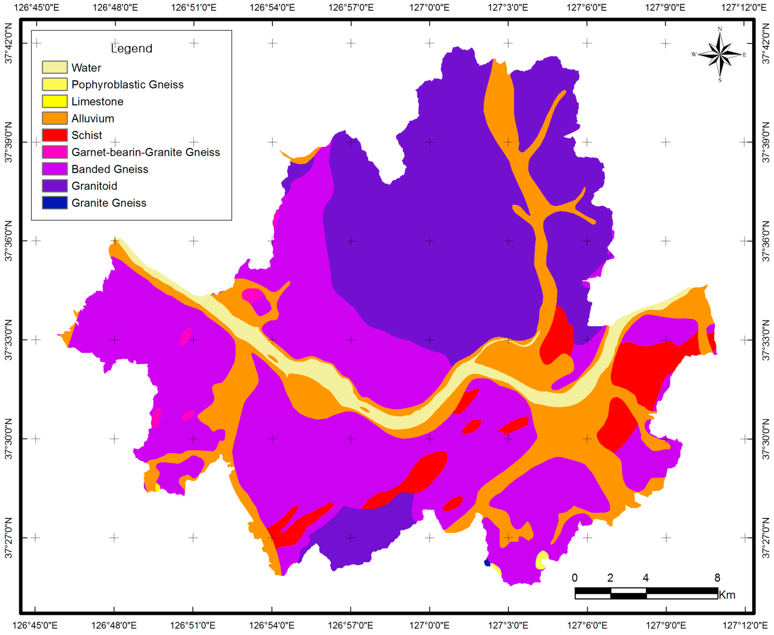
Figure 3.
Spatial database for flood-susceptibility analysis: (a) ground elevation; (b) slope gradient; (c) SLF; (d) TWI; (e) SPI; (f) distance from the water; (g) type of impermeable land use; (h) type of agricultural land use; (i) retarding basin; (j) soil drainage.
Figure 3.
Spatial database for flood-susceptibility analysis: (a) ground elevation; (b) slope gradient; (c) SLF; (d) TWI; (e) SPI; (f) distance from the water; (g) type of impermeable land use; (h) type of agricultural land use; (i) retarding basin; (j) soil drainage.
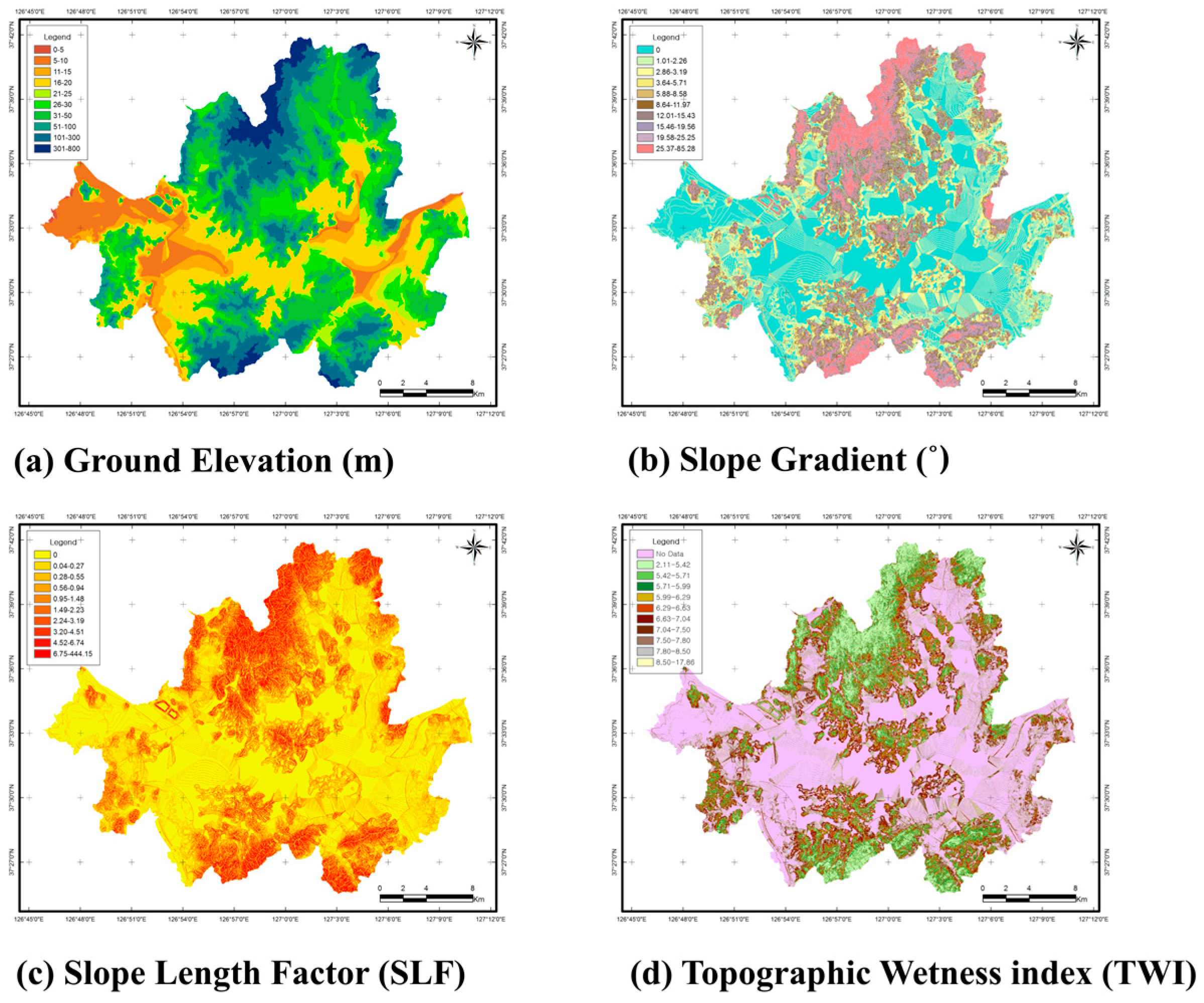

Figure 4.
Flowchart outlining the methodology of this study.
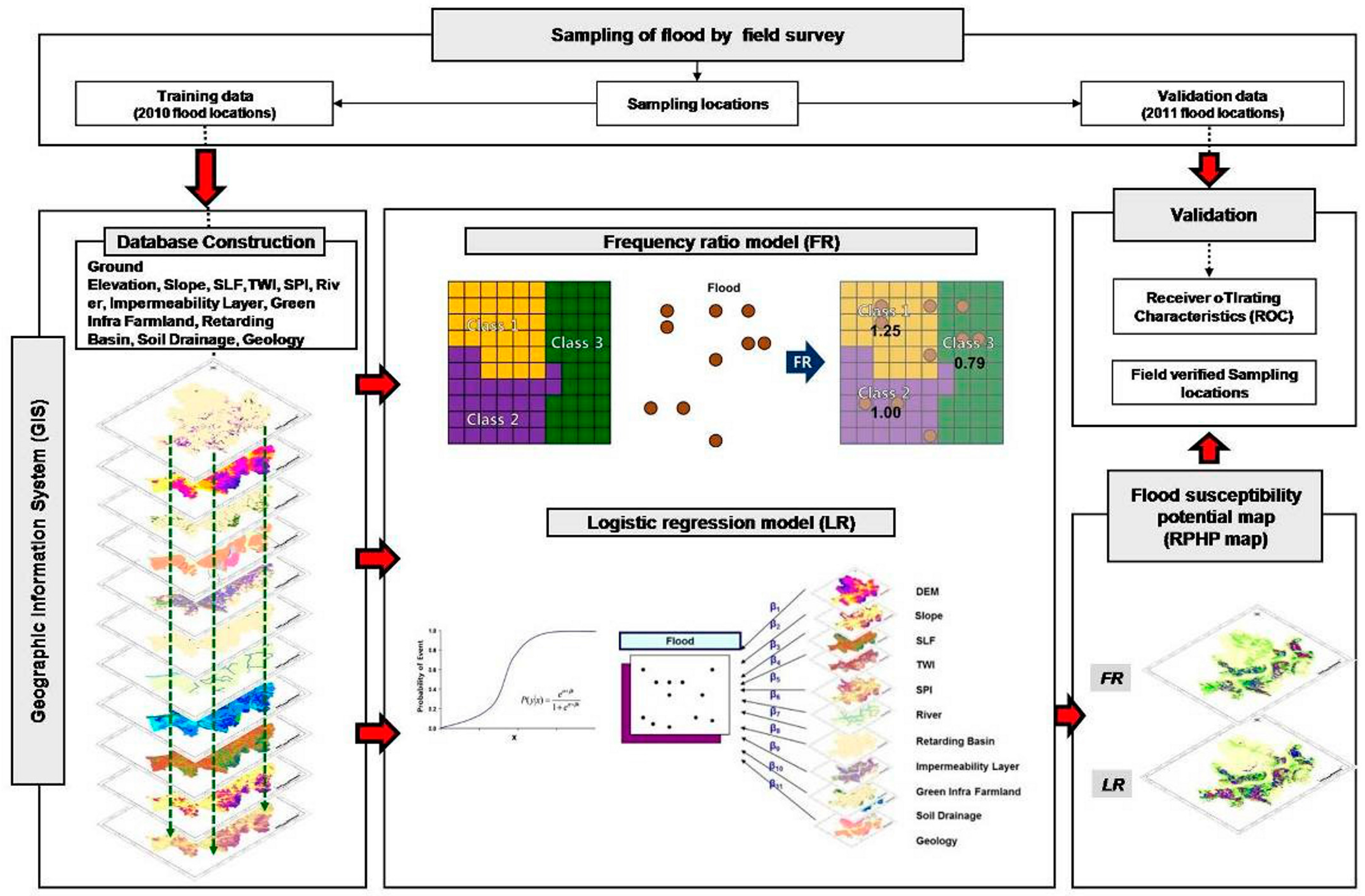
Figure 5.
Flood susceptibility maps: (a) Frequency Ratio (FR); (b) Logistic Regression (LR).
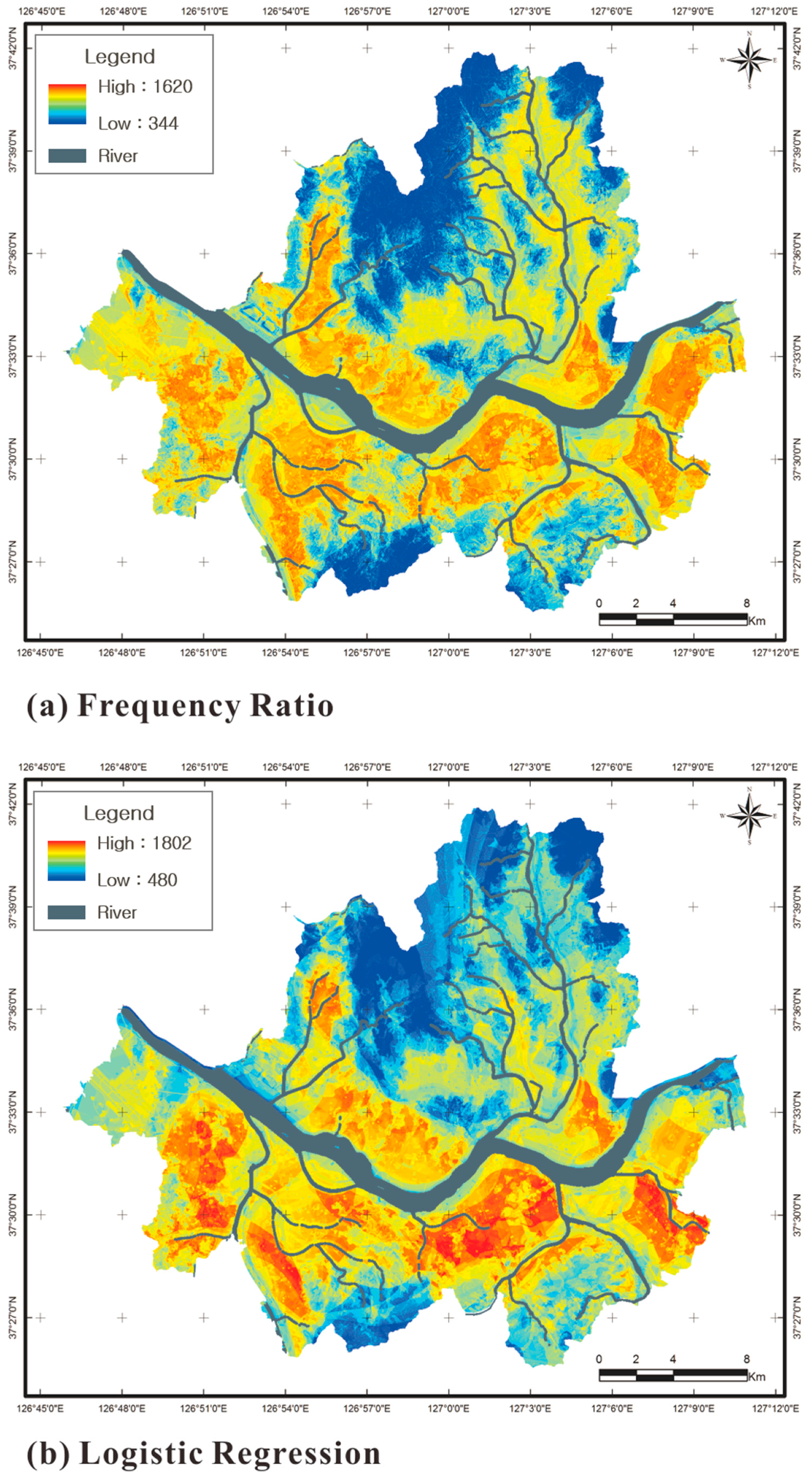
Figure 6.
Cumulative frequency diagram showing flood susceptibility index rank (X-axis) as a cumulative percentage of flood occurrence (Y-axis).
Figure 6.
Cumulative frequency diagram showing flood susceptibility index rank (X-axis) as a cumulative percentage of flood occurrence (Y-axis).

Table 1.
Data layer describing the flooded area within the study region.
| Category | Factors | Data Type | Scale |
|---|---|---|---|
| Hazard (inundation trace map) a | Flooded area | Polygon | 1:1000 |
| Topographic map b | Ground elevation (m) | GRID | 1:1000 |
| Slope (°) | |||
| Slope length factor (SLF) | |||
| Topographic wetness index (TWI) | |||
| Stream power index (SPI) | |||
| Distance from the river | |||
| Land use and land registration map | Type of impermeable land use | Polygon | 1:25,000 |
| Type of agricultural land use | |||
| Retarding basin | |||
| Soil map c | Soil drainage | Polygon | 1:25,000 |
| Geological map d | Geology | Polygon | 1:25,000 |
a Inundation trace map produced by the Ministry of Public Safety and Security (MPSS); b topographical factors were extracted from the digital topographic map by National Geographic Information Institute (NGII); c detailed soil map produced by the Rural Development Administration (RDA); d geological map produced by the Korea Institute of Geoscience & Mineral Resource (KIGAM).
Table 2.
Frequency ratios for flooding and related factors.
| Factor | Class | No. of Flood | % of Flood | No. of Pixels in Domain b | % of Pixels in Domain | Frequency Ratio |
|---|---|---|---|---|---|---|
| Ground elevation (m) | 0−5 | 0 | 0.00 | 8430 | 0.14 | 0.00 |
| 5−10 | 8118 | 6.39 | 489,094 | 8.06 | 0.79 | |
| 11−15 | 4391 | 3.46 | 403,484 | 6.65 | 0.52 | |
| 16−20 | 33,072 | 26.02 | 1,015,155 | 16.72 | 1.56 | |
| 21−25 | 12,763 | 10.04 | 361,080 | 5.95 | 1.69 | |
| 26−30 | 22,342 | 17.58 | 706,376 | 11.64 | 1.51 | |
| 31−50 | 37,396 | 29.43 | 1,230,145 | 20.27 | 1.45 | |
| 51−100 | 7518 | 5.92 | 896,300 | 14.77 | 0.40 | |
| 101−300 | 1487 | 1.17 | 750,673 | 12.37 | 0.09 | |
| 301−800 | 0 | 0.00 | 208,967 | 3.44 | 0.00 | |
| Slope gradient (˚) | 0 | 59,623 | 46.90 | 2,521,876 | 41.55 | 1.13 |
| 1.01−2.26 | 14,151 | 11.19 | 478,891 | 7.89 | 1.42 | |
| 2.86−3.19 | 17,565 | 13.84 | 591,965 | 9.75 | 1.42 | |
| 3.64−5.71 | 10,596 | 8.32 | 380,452 | 6.27 | 1.33 | |
| 5.88−8.58 | 7725 | 6.07 | 362,489 | 5.97 | 1.02 | |
| 8.64−11.97 | 5667 | 4.45 | 350,639 | 5.78 | 0.77 | |
| 12.01−15.43 | 4571 | 3.59 | 348,487 | 5.74 | 0.63 | |
| 15.46−19.56 | 3779 | 2.97 | 347,157 | 5.72 | 0.52 | |
| 19.58−25.25 | 2557 | 2.01 | 344,189 | 5.67 | 0.35 | |
| 25.37−85.28 | 853 | 0.67 | 343,559 | 5.66 | 0.12 | |
| SLF | 0 | 77,724 | 61.03 | 3,409,873 | 56.18 | 1.09 |
| 0.04−0.27 | 9290 | 7.29 | 299,029 | 4.93 | 1.48 | |
| 0.28−0.55 | 9118 | 7.16 | 300,560 | 4.95 | 1.45 | |
| 0.56−0.94 | 8095 | 6.36 | 296,277 | 4.88 | 1.30 | |
| 0.95−1.48 | 6809 | 5.35 | 300,512 | 4.95 | 1.08 | |
| 1.49−2.23 | 5331 | 4.19 | 295,857 | 4.87 | 0.86 | |
| 2.24−3.19 | 4218 | 3.31 | 293,309 | 4.83 | 0.69 | |
| 3.20−4.51 | 3281 | 2.58 | 292,385 | 4.82 | 0.53 | |
| 4.52−6.74 | 2315 | 1.82 | 290,981 | 4.79 | 0.38 | |
| 6.75−444.15 | 1167 | 0.92 | 290,921 | 4.79 | 0.19 | |
| TWI | No Data | 67,183 | 53.10 | 2,522,124 | 41.55 | 1.28 |
| 2.11−5.42 | 857 | 0.68 | 355,330 | 5.85 | 0.12 | |
| 5.42−5.71 | 1697 | 1.34 | 354,821 | 5.85 | 0.23 | |
| 5.71−5.99 | 2317 | 1.83 | 355,598 | 5.86 | 0.31 | |
| 5.99−6.29 | 2960 | 2.34 | 354,962 | 5.85 | 0.40 | |
| 6.29−6.63 | 4303 | 3.40 | 355,132 | 5.85 | 0.58 | |
| 6.63−7.04 | 6996 | 5.53 | 368,520 | 6.07 | 0.91 | |
| 7.04−7.50 | 8977 | 7.10 | 351,981 | 5.80 | 1.22 | |
| 7.50−7.80 | 10,745 | 8.49 | 350,659 | 5.78 | 1.47 | |
| 7.80−8.50 | 10,677 | 8.44 | 350,360 | 5.77 | 1.46 | |
| 8.50−17.86 | 9811 | 7.75 | 350,225 | 5.77 | 1.34 | |
| SPI | 0 | 77,724 | 61.16 | 3,409,873 | 56.18 | 1.09 |
| 0.02−0.14 | 8963 | 7.05 | 295,658 | 4.87 | 1.45 | |
| 0.14−0.26 | 7417 | 5.84 | 315,328 | 5.20 | 1.12 | |
| 0.26−0.41 | 5707 | 4.49 | 293,156 | 4.83 | 0.93 | |
| 0.41−0.60 | 5341 | 4.20 | 292,847 | 4.82 | 0.87 | |
| 0.60−0.83 | 4959 | 3.90 | 293,017 | 4.83 | 0.81 | |
| 0.83−1.12 | 4620 | 3.64 | 293,265 | 4.83 | 0.75 | |
| 1.12−1.50 | 4343 | 3.42 | 292,669 | 4.82 | 0.71 | |
| 1.50−2.20 | 4372 | 3.44 | 292,165 | 4.81 | 0.71 | |
| 2.20−11.82 | 3902 | 3.07 | 291,726 | 4.81 | 0.64 | |
| Distance from the river | No Data | 123,744 | 97.12 | 5,289,682 | 87.15 | 1.11 |
| 10 m buffer | 552 | 0.43 | 384,501 | 6.33 | 0.07 | |
| 50 m buffer | 1288 | 1.01 | 183,258 | 3.02 | 0.33 | |
| 100 m buffer | 1835 | 1.44 | 212,271 | 3.50 | 0.41 | |
| Type of impermeable land use | No data | 24,032 | 18.86 | 2,434,555 | 0.47 | 40.11 |
| Residential area | 50,141 | 39.35 | 1,779,996 | 1.34 | 29.33 | |
| Manufacturing area | 769 | 0.60 | 50,322 | 0.73 | 0.83 | |
| Commercial area | 19,455 | 15.27 | 521,668 | 1.78 | 8.59 | |
| Recreational area | 592 | 0.46 | 56,468 | 0.50 | 0.93 | |
| Trafficked area | 21,837 | 17.14 | 734,043 | 1.42 | 12.09 | |
| Public area | 10,593 | 8.31 | 492,660 | 1.02 | 8.12 | |
| Type of agricultural land use | Non-green farm | 119,531 | 93.81 | 5,122,219 | 84.39 | 1.11 |
| Paddy | 686 | 0.54 | 99,829 | 1.64 | 0.33 | |
| Field | 1188 | 0.93 | 144,320 | 2.38 | 0.39 | |
| Orchard | 0 | 0.00 | 3745 | 0.06 | 0.00 | |
| Other plantations | 0 | 0.00 | 1649 | 0.03 | 0.00 | |
| Natural grassland | 31 | 0.02 | 5401 | 0.09 | 0.27 | |
| Grassland | 2457 | 1.93 | 476,247 | 7.85 | 0.25 | |
| Barren ground | 3526 | 2.77 | 216,302 | 3.56 | 0.78 | |
| Retarding Basin | No data | 127,335 | 99.93 | 6,054,729 | 99.75 | 1.00 |
| Retarding basin | 84 | 0.07 | 14,983 | 0.25 | 0.27 | |
| Soil drainage | No data | 705 | 0.55 | 634,006 | 10.45 | 0.05 |
| Poorly drained | 3216 | 2.53 | 118,688 | 1.96 | 1.29 | |
| Somewhat poorly drained | 32,832 | 25.83 | 1,270,310 | 20.93 | 1.23 | |
| Moderately well drained | 73,913 | 58.16 | 2,122,951 | 34.98 | 1.66 | |
| Very well drained | 16,421 | 12.92 | 1,923,788 | 31.69 | 0.41 | |
| Geology | Water | 214 | 0.17 | 258,197 | 4.25 | 0.04 |
| Pophyroblastic gneiss | 0 | 0.00 | 6595 | 0.11 | 0.00 | |
| Limestone | 0 | 0.00 | 1061 | 0.02 | 0.00 | |
| Alluvium | 15,093 | 11.85 | 1,083,285 | 17.85 | 0.66 | |
| Schist | 12,946 | 10.16 | 303,291 | 5.00 | 2.03 | |
| Garnet-bearing-granite gneiss | 779 | 0.61 | 20,736 | 0.34 | 1.79 | |
| Banded gneiss | 92,726 | 72.77 | 2,428,763 | 40.01 | 1.82 | |
| Granitoid | 5661 | 4.44 | 1,966,740 | 32.40 | 0.14 | |
| Granite gneiss | 0 | 0.00 | 1044 | 0.02 | 0.00 |
Table 3.
The output of logistic regression analysis.
| Factor | B | S.E | Wals | Sig. | |
|---|---|---|---|---|---|
| Ground elevation (m) | −0.007 | 0.000 | 273.401 | 0.000 | |
| Slope gradient (°) | −0.005 | 0.002 | 4.284 | 0.038 | |
| SLF | −0.006 | 0.008 | 0.663 | 0.416 | |
| TWI | 0.020 | 0.003 | 57.420 | 0.000 | |
| SPI | −0.025 | 0.017 | 2.054 | 0.152 | |
| Distance from the river | 0.001 | 0.000 | 3978.433 | 0.000 | |
| Type of impermeable land use | No data | −0.229 | 0.033 | 717.704 | 0.000 |
| Residential area | 0.156 | 0.028 | |||
| Manufacturing area | −0.440 | 0.086 | |||
| Commercial area | 0.489 | 0.032 | |||
| Recreational area | −0.116 | 0.095 | |||
| Trafficked area | 0.180 | 0.031 | |||
| Public area | 0.000 | 0.000 | |||
| Type of agricultural land use | Non-green farm | −0.079 | 0.050 | 517.979 | 0.000 |
| Paddy | −1.814 | 0.106 | |||
| Field | −1.171 | 0.084 | |||
| Orchard | −16.906 | 1901.109 | |||
| Other plantations | −17.699 | 2883.907 | |||
| Natural grassland | −0.525 | 0.385 | |||
| Grassland | −0.252 | 0.068 | |||
| Barren ground | 0.000 | 0.000 | |||
| Retarding basin | No data | 1.485 | 0.335 | 19.647 | 0.000 |
| Retarding basin | 0.000 | 0.000 | |||
| Soil drainage | No data | −1.215 | 0.092 | 1048.151 | 0.000 |
| Poorly drained | 0.383 | 0.065 | |||
| Somewhat poorly drained | 0.400 | 0.025 | |||
| Moderately well drained | 0.579 | 0.022 | |||
| Very well drained | 0.000 | 0.000 | |||
| Geology | Water | 14.116 | 3789.108 | 3854.436 | 0.000 |
| Pophyroblastic gneiss | 0.056 | 4055.009 | |||
| Limestone | −1.683 | 5242.473 | |||
| Alluvium | 16.177 | 3789.108 | |||
| Schist | 16.657 | 3789.108 | |||
| Garnet-bearing-granite gneiss | 16.653 | 3789.108 | |||
| Banded gneiss | 16.755 | 3789.108 | |||
| Granitoid | 14.893 | 3789.108 | |||
| Granite gneiss | 0.000 | 0.000 | |||
© 2018 by the authors. Licensee MDPI, Basel, Switzerland. This article is an open access article distributed under the terms and conditions of the Creative Commons Attribution (CC BY) license (http://creativecommons.org/licenses/by/4.0/).
Share and Cite
MDPI and ACS Style
Lee, S.; Lee, S.; Lee, M.-J.; Jung, H.-S. Spatial Assessment of Urban Flood Susceptibility Using Data Mining and Geographic Information System (GIS) Tools. Sustainability 2018, 10, 648. https://doi.org/10.3390/su10030648
AMA Style
Lee S, Lee S, Lee M-J, Jung H-S. Spatial Assessment of Urban Flood Susceptibility Using Data Mining and Geographic Information System (GIS) Tools. Sustainability. 2018; 10(3):648. https://doi.org/10.3390/su10030648
Chicago/Turabian StyleLee, Sunmin, Saro Lee, Moung-Jin Lee, and Hyung-Sup Jung. 2018. "Spatial Assessment of Urban Flood Susceptibility Using Data Mining and Geographic Information System (GIS) Tools" Sustainability 10, no. 3: 648. https://doi.org/10.3390/su10030648
Note that from the first issue of 2016, this journal uses article numbers instead of page numbers. See further details here.