Towards a Smart City: Development and Application of an Improved Integrated Environmental Monitoring System


Department of Land Surveying and Geo-informatics, The Hong Kong Polytechnic University, Hong Kong, China
*
Author to whom correspondence should be addressed.
Sustainability 2018, 10(3), 623; https://doi.org/10.3390/su10030623
Submission received: 16 January 2018
/
Revised: 14 February 2018
/
Accepted: 15 February 2018
/
Published: 28 February 2018
(This article belongs to the Special Issue Spatial and Spatio-Temporal Planning for Urban Health and Sustainability)
Abstract
:Environmental deprivation is an issue influencing the urban wellbeing of a city. However, there are limitations to spatiotemporally monitoring the environmental deprivation. Thus, recent studies have introduced the concept of “Smart City” with the use of advanced technology for real-time environmental monitoring. In this regard, this study presents an improved Integrated Environmental Monitoring System (IIEMS) with the consideration on nine environmental parameters: temperature, relative humidity, PM2.5, PM10, CO, SO2, volatile organic compounds (VOCs), UV index, and noise. This system was comprised of a mobile unit and a server-based platform with nine highly accurate micro-sensors in-coupling into the mobile unit for estimating these environmental exposures. A calibration test using existing monitoring station data was conducted in order to evaluate the systematic errors. Two applications with the use of the new system were also conducted under different scenarios: pre- and post-typhoon days and in areas with higher and lower vegetation coverage. Linear regressions were applied to predict the changes in environmental quality after a typhoon and to estimate the difference in environmental exposures between urban roads and green spaces. The results show that environmental exposures interact with each other, while some exposures are also controlled by location. PM2.5 had the highest change after a typhoon with an estimated 8.0 μg/m³ decrease that was controlled by other environmental factors and geographical location. Sound level and temperature were significantly higher on urban roads than in urban parks. This study demonstrates the potential to use IIEMS for environmental quality measurements under the greater framework of a Smart City and for sustainability research.
1. Introduction
Urban inhabitants are more exposed to adverse environments with diversified deprivation, including extremes in humiture (a combination of temperature and humidity), air pollutants, ultra-violet (UV) radiation, and noise. These extremes in environmental deprivation can influence human health; for example, extremes in temperature have increased morbidity and mortality risk [1,2] and air pollution from carbon monoxide (CO), sulfur dioxide (SO2), and particulate matter (PM) have been found to be associated with cardiovascular and respiratory issues [3,4,5,6,7,8,9]. These environmental deprivations can also influence health risk in both spatial and temporal dimensions [10,11,12,13,14,15]. Thus, spatiotemporally monitoring changes in environmental deprivation is critical [16], especially to target environmentally deprived areas during sustainability planning.
Traditionally, monitoring these environmental deprivations have been dependent on government-based stations. However, these stations are usually sparsely distributed; as a result, the data from these stations may not be able to provide micro-scale environmental information for individual-level health assessments [17]. To improve this issue, several studies have applied moderate-resolution satellite images to estimate the spatial variability of environmental deprivation [18,19,20,21,22,23] and relate this spatial variability to health risk areas [24,25,26,27,28]. Unfortunately, the orbits of satellites restrict the days of overpass and limit the ability to conduct a nearly real-time measurement of environmental deprivation. Therefore, advanced concepts such as “volunteered geographic information” [29] and “Smart City” [30] have been proposed for increasing the potential number of sensors across districts/areas in order to improve the real-time monitoring of environment exposure and to enhance the protocols for sustainable planning.
2. Towards a Smart City
Moving towards the new era of innovative and advanced technologies, a new concept called “Smart City” has been proposed [30]. The major key to a Smart City’s framework is to use extensive networks of portable and integrated environmental monitoring systems for monitoring near real-time environmental changes across an urban environment. In the extension of a Smart City’s framework, the environmental monitoring networks can link to cloud computing [31,32,33] for disseminating useful information to the end-user in near real-time (e.g., people who use smartphones). Therefore, in order to conduct this spatiotemporal measurement with near real-time technologies, improvements in older technologies has become a necessity in this field. As a result, several environmental sensing projects have recently been proposed, particularly those for improvements in the smart technologies for air quality monitoring. One of the frontier projects was an integrated platform developed by N-SMARTS, which used temperature, CO, and nitrogen oxide (NOx) sensors and a GPS-embedded phone [34]. This integrated platform applied Bluetooth technology to connect sensors and mobile phones. Another project of environmental monitoring was the “MobGeoSen” system, which was first conducted by Kanjo et al. [35]. This monitoring system consisted of a sound-level sensor in a mobile phone with a data logger, a GPS receiver, and a Bluetooth communication module. Advancing from these projects, Common Sense developed a handheld monitor that measured CO, NOx, ozone (O3), temperature, and humidity [36]. This handheld monitor also included a radio for General Packet Radio Service (GPRS) and a GPS receiver, which allowed for the sensor data to be uploaded to a hosted server for web-based dissemination, visualization, and analysis. Similar techniques have been applied to other projects, including assembling temperature and electrochemical sensors (CO, NO and NO2), GPS, and GPRS modules on mobile devices for monitoring urban air quality [37]. It also used GPS and Global System for Mobile (GSM) communication modules with temperature, humidity, NO2, CO, and PM2.5 sensors for air sensing system development [38]. However, these integrated systems were incomprehensive and ineffective for monitoring the urban environment due to critical environmental factors such as volatile organic compounds (VOCs), UV, and noise, which were commonly excluded from the system design. In addition, some function modules such as GPS or network connections were independent of the whole monitoring system and caused redundancy in system structure.
To resolve these technical issues for building a better environmental monitoring network under the framework of a Smart City, this study aims to develop an innovative platform based on the former development of a Personal Integrated Environmental Monitoring System from Wong et al. [39]. Personal Integrated Environmental Monitoring System (IEMS) is a portable and compact device, consisting of a microcontroller, environmental sensors, and an extra smartphone with Bluetooth communication module components. The newly developed system has been enhanced both in hardware and software aspects. The advantages of this new system include: (i) comprehensive monitoring of the urban environment based on nine parameters (temperature, relative humidity, PM2.5, PM10, CO, SO2, VOC, UV, and noise); (ii) a more concise and effective system structure by integrating all of the sensors into a single unit; and (iii) the use of sensors with higher accuracy to differentiate the microscale changes of environmental quality. These advantages not only enable the improved IEMS (hereafter IIEMS) to monitor the environmental quality but also improve the data collection for analyzing the impacts of environmental exposures due to spatiotemporal changes of the geophysical environment.
To evaluate the potential uses of IIEMS for environmental analyses and sustainable planning, two case studies were conducted with field measurements using IIEMS: (i) a case study of typhoon days and (ii) a case study of urban roads and parks. For (i), a typhoon, also known as a tropical cyclone, is a severe weather event that brings heavy rain, strong winds, and large storm surges during the moment of landfall [40]. This extreme weather may lead to significant changes in environmental exposures during the post-event period. For (ii), vegetation cover has been identified as the landscape that can reduce temperature and environmental pollution [41,42]. With the use of IIEMS, it is expected that fine spatiotemporal changes in environmental exposures can be measured, and the detailed impact of the geophysical environment on air quality for sustainable planning can be estimated.
In conclusion, the main objective of this study is to develop a new generation of IEMS and to apply this IIEMS to multiple urban environmental studies, with consideration on the impact of the geophysical environment for sustainable planning.
3. Development of Smart Technology: An Improved Integrated Environmental Monitoring System
3.1. System Architecture
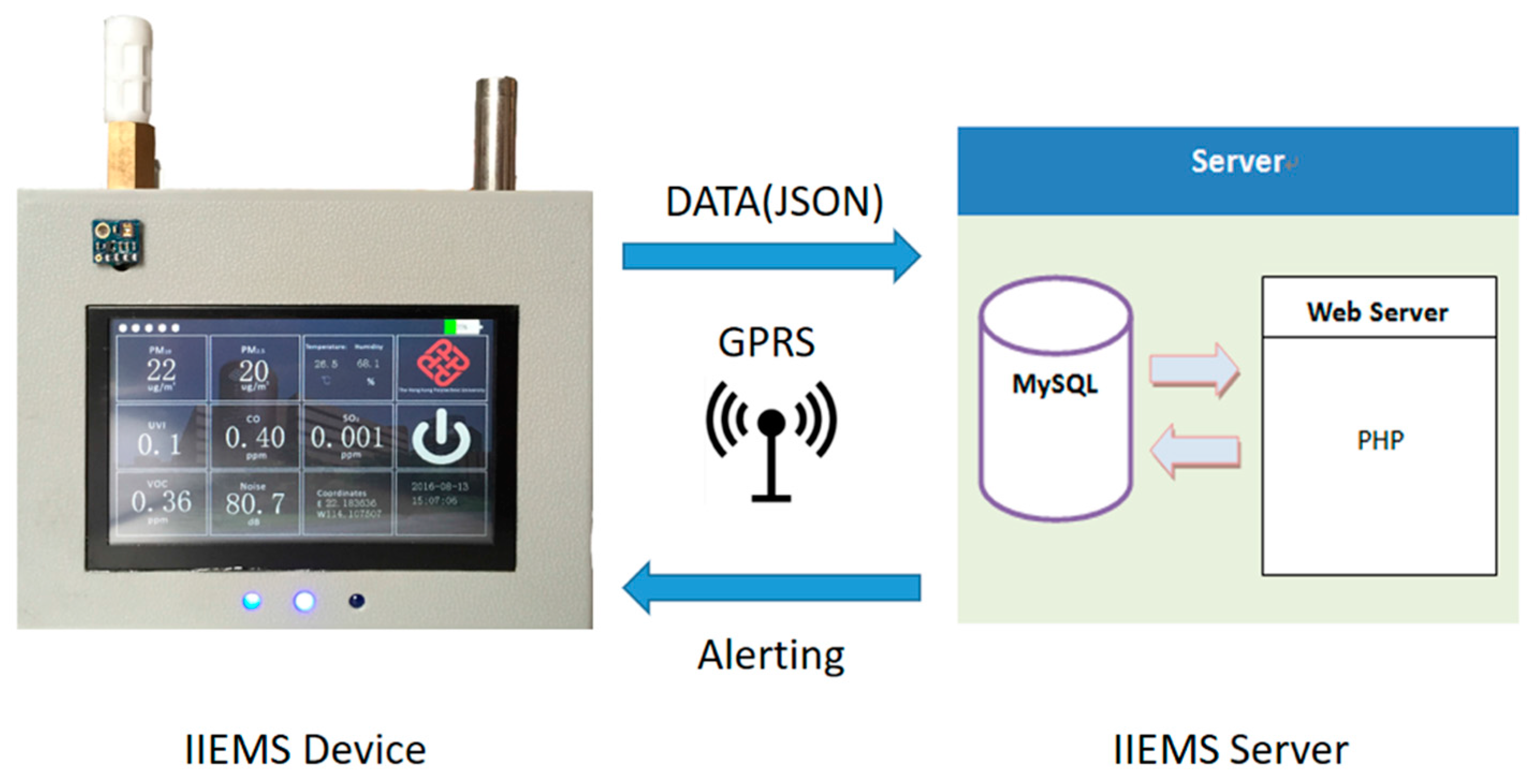
The entire structure of IIEMS, as presented in Figure 1, is comprised of two major components: an IIEMS mobile unit and an IIEMS server. This device is equipped with nine sensors to retrieve the data of each environmental parameter. Once the device receives data, it will send the signal in JavaScript Object Notation (JSON) format via the power-on self-test (POST) service through a wireless service to the server. Data will be stored in a web database for further long-term data analysis and it can be displayed on a website or on a mobile application.
This device is developed and designed with: (i) a mobile unit that is handheld and lightweight, which enables field tests; (ii) wireless data communication capabilities for real-time data collection including environment data, such as spatiotemporal information; (iii) a high level of integration of sensors to measure the environmental indices, including temperature, relative humidity, air pollutants, UV, and noise; (iv) an accurate GPS positioning module to acquire the geographical location in real time; and (v) adequate battery power for long-term remote operation in the field. Table 1 gives the technical specifications of the IIEMS configuration scheme.
3.2. Calibration Tests
Most sensors are calibrated in a laboratory before assembling. However, some high-resolution sensors such as CO, SO2, and particulate matter sensors can be influenced by practical conditions; hence, evaluation and re-calibration of the device while considering their field performances are essential. Data from the roadside Air Quality Monitoring Station (AQMS) in Mong Kok, Hong Kong, operated by the Hong Kong Environmental Protection Department (EPD) was selected as a reference for calibration. The AQMS is located at the junction of Nathan Road and Lai Chi Kok Road, which are roads with heavy traffic. An IIEMS device was deployed near the station and field calibration tests were carried out intermittently between 18 July 2016 and 22 August 2016. There were a total of 18 discontinuous hours of data for calibration because the battery of the device needed to be recharged from time to time. Moreover, parameters were sometimes undetectable since their concentrations were lower than the sensor’s detection limits. The raw data from the device were transmitted in near real-time to the server located at the Hong Kong Polytechnic University in 10-s intervals; then, the data were processed into average hourly data. In addition, hourly-based AQMS data for PM2.5, PM10, CO, and SO2 were obtained from the HKEPD website [43].
A linear regression model was established with IIEMS data and reference station data. The calibration curve was derived for each parameter. A verification test was conducted to validate the performance of IIEMS. Ten-hour valid data were used in this test.
Mean absolute error (MAE) and mean relative error (e.g., mean absolute percentage error, MRE) were used to evaluate the field performance of the IIEMS device [44,45]. These two indicators are defined as follows:
where fi is the forecast value, yi is the actual value of the quantity being forecast, and n is the number of different times for which the variable is forecast.
4. Application of the Improved Integrated Environmental Monitoring System
4.1. Study Site
In order to evaluate the accuracy of IIEMS for environmental monitoring and sustainable urban planning, two case studies were applied at the Kowloon Peninsula of Hong Kong. In brief, Kowloon Peninsula of Hong Kong is an urban area with a compact city setting [46]. The urban morphology of this compact city can block ventilation, resulting to spatial variation and urban microclimates in different neighborhoods with different land uses. The city is also influenced by a subtropical climate in which extreme days such as typhoons can affect the wind profiles across the city [47] and this can further influence the variations in the urban microclimates. Thus, there are also studies on how public perceptions of climate change can reshape the function of green environments across this city [48]. Therefore, it is important to conduct tests for both typhoon/non-typhoon days and green/non-green environments for the application of IIEMS for environmental monitoring and city planning under the greater framework of a Smart City in the future.
4.2. Typhoon Tests
The first application of this study was to evaluate the influence of severe weather on environmental quality based on IIEMS data. This study was conducted on the day before and the day after Typhoon Nida. Typhoon Nida, also known as “Severe Tropical Storm Carina” in the Philippines, was a category I typhoon (based on Saffir–Simpson scale) that struck Luzon Island in the Philippines during late July 2016, and influenced Guangdong, China, in early August 2016 [49]. Before the landfall of Typhoon Nida, the Hong Kong Observatory first released a “strong wind” signal (No. 3 signal) at 11:40 on 2 August 2016; then, the Hong Kong Observatory raised the signal to “gale or storm” signal (No. 8 signal) at 20:40 on 2 August 2016. All tropical cyclone warning signals were cancelled at 17:40 on 3 August 2016.
There were two field measurements for this typhoon test. The first one was conducted during the pre-typhoon period on 1 August 2016, from 13:56:50 to 14:49:58, and the second was conducted during the post-typhoon period on 3 August 2016, from 14:10:59 to 14:54:55. All measurements were taken along Nathan Road, a main road with heavy traffic, using the IIEMS device. The trail of two measurements was started at the Exit D1 of the Tsui Sha Tsui Metro Station (22.298° N, 114.172° E) and ended at the last junction at the northern part of Nathan Road (22.326° N, 114.168° E) with a total distance of 4.68 km. The measurements were conducted by a volunteer holding the IIEMS device and walking with a constant step frequency along the west pavement of Nathan Road.
A linear regression approach was applied to estimate the change in environmental quality after Typhoon Nida and four sets of models were developed. The first set of models was used to estimate the crude change in environmental quality after the typhoon. This approach assumed that environmental factors did not influence or interact with other environmental factors. Each environmental parameter was, therefore, assigned as a separate dependent variable while a binary variable indicating day before/after the typhoon was assigned as the independent variable. In contrast, the second set of models assumed that all environment parameters were somehow influencing other environmental parameters during a severe weather event and, therefore, all environmental parameters except the one used as the dependent variable were included in the regression as independent variables. This selection of independent variables was also used for the purpose of estimating the independent effect of temporal change after the landfall of the typhoon, controlled by a comprehensive geophysical environment. The third set of models was developed based on the first set of models with the additional parameters of latitude and longitude as controls. It was assumed that the location of each measurement should influence the environmental exposures but the influence remained unknown. The fourth set of models was the comprehensive model controlled by all environmental parameters, latitude, and longitude, assuming all components of the urban environment were spatially interacting with the others. The Akaike information criterion (AIC) of each model was reported to compare the model accuracies. Based on the AIC results, the best model with the lowest AIC for each environmental parameter was selected and the independent effect and 95% confidence interval (CI) of the temporal change on environmental exposure are reported.
4.3. Urban Road/Park Tests
The second application of IIEMS was the evaluation of the difference between landscapes with less and more vegetation. Therefore, Kowloon Park in Tsim Sha Tsui was selected to be the site of an “urban park” test. This park is one of the largest urban parks in Hong Kong, with extensive smoke-free areas and a high coverage of vegetation. This park is also adjacent to Nathan Road. The field measurement was conducted on 13 August 2016, between 10:52:06 and 11:16:10. This trail started at the South Gate of Kowloon Park (22.298° N, 114.170° E) with a volunteer holding the IIEMS device and walking across Kowloon Park with a constant step frequency. This volunteer then walked on Austin Road and Nathan Road, two main roads in Kowloon, until Exit C of Yau Ma Tei Metro Station (22.312° N, 114.171° E). The total distance of this test trail is 1.23 km.
A similar linear approach as the typhoon test with four sets of models was applied to test the environmental influence of the park and roads on environmental quality. A binary independent variable specific to the urban park test was applied in this case study. Data retrieved next to the road were assigned as “1” while data obtained within the park were assigned as “0”. The results of these four models indicate the independent effect of the environmental differences between urban roads and park on the environmental exposure.
5. Results
5.1. Calibration of IIEMS
Four calibrations were conducted in this study, including the field calibration results of CO (Figure 2), SO2 (Figure 3), PM10, and PM2.5 (Figure 4). There is consistency in the variations and a similar trend between CO data from IIEMS collections and EPD (Figure 2a) and also for SO2, PM10, and PM2.5 (Figure 3a and Figure 4a). In addition, SO2 data from IIEMS were generally lower than the data from EPD while the other data from IIEMS were generally higher than the EPD data. The CO sensor had the highest accuracy for which MAE and MRE of CO were 0.07 ppm and 16.20% when the EPD average CO concentration was 0.43 ppm. The PM sensor also provided data with accuracy. MAE and MRE of PM10 were 4.21 μg/m³ and 18.79% when the EPD average was about 22.56 μg/m³, and the MAE and MRE of PM2.5 were 3.55 μg/m³ and 28.02% when the average was 14.61 μg/m³. In contrast, MAE and MRE of SO2 were 0.06 ppb and 47.89% when the EPD average of the SO2 concentration was 0.18 ppb, indicating a significant systematic error.
By applying the calibration curves for the data from all sensors, the R2 of CO, SO2, PM10, and PM2.5 were 0.72, 0.86, 0.70, and 0.73, respectively. This showed that data from the IIEMS sensors and EPD were highly correlated. A verification test was conducted with the EPD data, raw IIEMS data, and calibrated IIEMS data. This test found an improvement in the IIEMS data after calibration. The MAE and MRE of calibrated CO and SO2 were 0.05ppm and 0.02 ppb, and 7.74% and 21.70% lower than the raw data of IIEMS when the average CO of EPD was 0.68 ppm (Figure 2c) and average SO2 was 0.07 ppb. Figure 4c shows the verification tests by comparing EPD data, raw IIEMS data, and calibrated data. The MAE was 5.68 μg/m³ for PM10 and 4.24 μg/m³ for PM2.5 when the actual average was about 31.14 μg/m³ for PM10 and 21.24 μg/m³ for PM2.5. The MRE was 20.09% for PM10 and 24.50% for PM2.5. After calibration, the MAE dropped to 2.50 μg/m³ for PM10 and 1.43 μg/m³ for PM2.5. The MRE also dropped to 8.49% for PM10 and 8.53% for PM2.5. The results show that the embedded sensors were able to monitor the field environment with reasonable accuracies.
5.2. Application I: Typhoon Tests
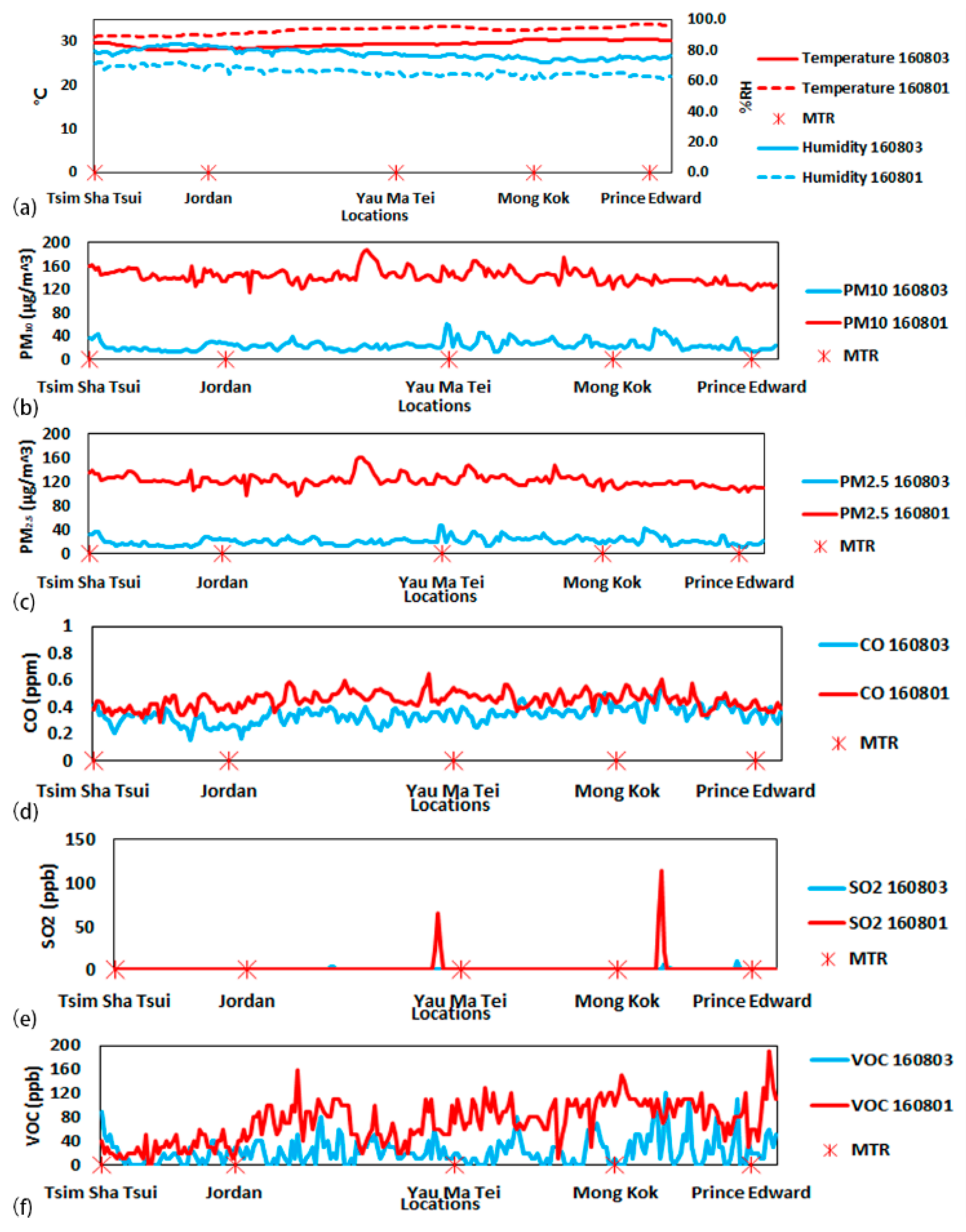
In general, Typhoon Nida brought cool weather and heavy precipitation to Hong Kong (Figure 5). The temperature during the post-typhoon period on Nathan Road dropped from 32.5 °C to 29.3 °C on average and the relative humidity increased from 65.9% to 77.55%. There were also significant decreases in PM10 and PM2.5 after the landfall of Typhoon Nida. PM10 dropped from 142 μg/m³ to 24 μg/m³ on average and PM2.5 dropped from 122 μg/m³ to 22 μg/m³, possibly due to high wind speeds and that heavy precipitation during the typhoon may have removed the particulate matter that had been trapped in the urban-built environment by poor air dispersion during days with low wind [50]. Hence, after the landfall of a typhoon, the air quality becomes better. This evidence also shows the general trend of other air pollutants where average CO, SO2, and VOC dropped from 0.45 ppm, 0.0014 ppm, and 0.071 ppm to 0.34 ppm, 0.00015 ppm, and 0.0019 ppm, respectively. However, these trends might also have been the result of dropping temperatures and humidity, which are highly associated with air pollution [51,52]. Anthropogenic factors may also have influenced the decreases in SO2 and VOC; for example, shutting down transportation services during the typhoon may have reduced the release of SO2 from vehicles and no construction being undertaken during the typhoon would have reduced the amount of formaldehyde emitted from decorative or building materials. This study has observed that spatial influences are one key to changing environment quality. Therefore, comparing simple models and comprehensive models for estimating environmental changes after a typhoon must also be conducted.
Based on AICs of each regression model (Table 2), all environmental parameters can influence each other while CO, temperature, relative humidity, VOC, noise, and UV are additionally controlled by the location. After adjusting all environmental or spatial factors with the best model (Table 3), CO, PM2.5, temperature, relative humidity, VOC, and UV were predicted to have significant changes after a typhoon event. The significant 8.0 μg/m³ decrease in PM2.5 after the typhoon event, controlled by all environmental factors, was expected. There was also a slight but significant decrease in temperature (−0.7 °C) and VOC (−0.05 ppm), controlled by all environmental factors and location, when the typhoon passed over Hong Kong. In contrast, the 5.9% increase in relative humidity and 0.7 increase in the UV index after the typhoon when controlled by other environmental factors and locations was expected. This result was possibly due to high evapotranspiration and cloud-free days after the heavy precipitation during the typhoon event. There was also a slight but significant increase of CO (0.1 ppm) after the typhoon event with the adjustments of all environmental and spatial factors.
5.3. Application II: Urban Road/Park Tests
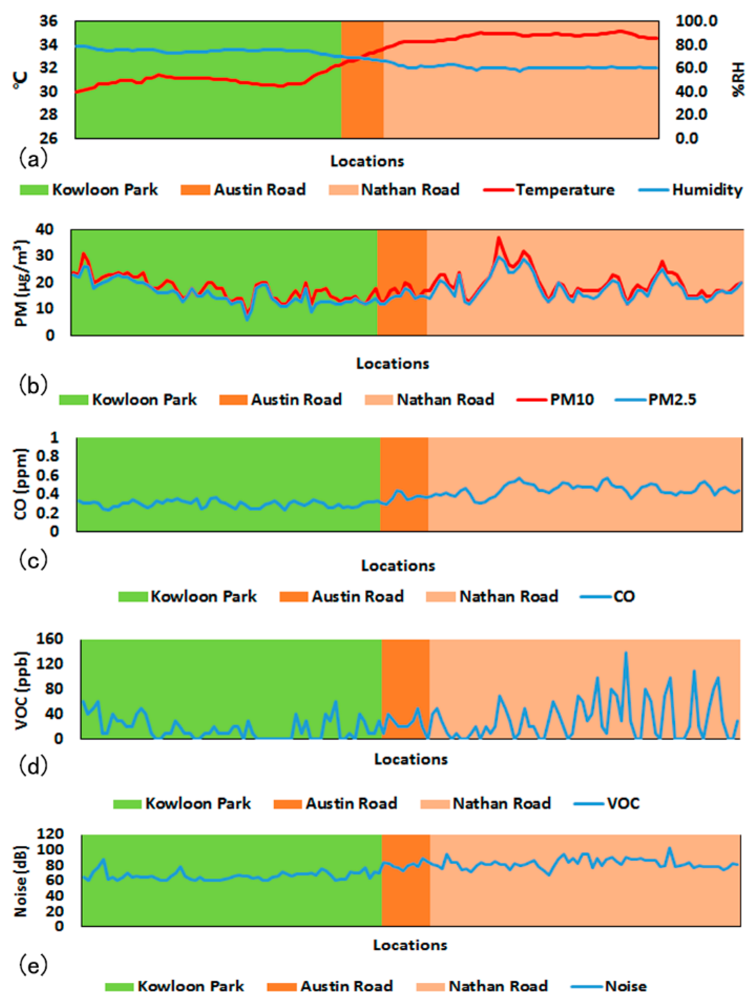
In general, the temperature on urban roads was significantly higher than within an urban park. The average temperature measurement across Kowloon Park was 30.9 °C, and it went up instantly to an average of 34.5 °C on the road (Figure 6). Relative humidity was also apparently higher in the park (74.9%) than on the road (61.8%) and noise across the park was averagely 15.7 dB lower than on the road. Also, PM10 and PM2.5 in the urban park were on average 1 μg/m³ and 2 μg/m³ lower, respectively, than on the road but the variations in PMs on the road were also high. For example, standard deviations of PM10 and PM2.5 on Nathan Road were 4.90 μg/m³ and 4.35 μg/m³, respectively. There were also slightly higher concentrations of CO and VOC on the road than within the park, which may be the result of the different nature of the environments or the influence of temperature and humidity. Further investigation with comprehensive modelling is, therefore, also needed to estimate the relationship between urban road/park and air quality.
Based on the AICs of the regression models (Table 4), all environmental parameters except noise were influenced by other factors, while PM2.5, temperature, noise, and UV were controlled by the geographic location in this case study. Adjusting to the environmental or spatial factors, temperature and noise had significant changes on urban roads (Table 5). Temperature was predicted to be 0.5 °C higher on the road, controlled by both environmental parameters and location. Noise on urban roads was 8.0 dB louder than in the urban park, controlled by location. The reductions in noise and temperature in the urban green space have been commonly found in global research and local studies [53,54,55,56,57].
6. Implications of Sustainable Planning with IIEMS
This study described the IIEMS system that was developed to meet the specified system and functional requirements. Some new developments of the IIEMS are described as follows: (i) the system is highly integrative without any other dependent component; (ii) the system has promising accuracy for monitoring an urban environment and has a portable size; (iii) all operations of the system perform well, observing real-time environmental changes with a simple and user-friendly interface on the device shell; and (iv) web and Android applications can be used anytime and anywhere. The applications of this study show the ability of microscale environmental measurements with IIEMS, especially in the two cases of this study: typhoon and urban road/park tests. This study also demonstrates the possibility for further extension of IIEMS to Smart City concept since environmental exposures such as air temperature and humidity can be spatiotemporally measured across land types and any change in land type is expected to induce a higher variation in the exposure [58,59]. In a high density-built environment such as Hong Kong, urban morphology can create a complex, block-level microclimate system with high variations of environmental exposures [60]. Previous studies have already demonstrated that mobile measurements could improve the spatiotemporal prediction of environmental quality [17,61], while this spatiotemporal prediction should be the key to accurately estimating the environmental health risk [16]. However, previous studies of mobile measurements were limited by field collection, which was labor dependent and, as a result, it was not easy to obtain high spatial coverage [62]. In contrast, IIEMS can be used as a tool for active volunteered geographic information (VGI) for building a Smart City. Active VGI allows public users to collect and share data for geographic use [29]. Previous projects such as Weather Underground [63] have promoted an active VGI scheme for weather data collection and have been successfully applied to global cities. However, one issue with such a project is that it requires participants to install weather stations at their homes. However, most people in high-density environments such as Hong Kong do not have enough space to install traditional, full-size equipment. With the use of IIEMS, it is believed that the participants could solve the issues above because the size of the IIEMS is small enough for installation. It can also be linked with top-down policies for installing smart sensors across neighborhoods, which has been done in other cities (e.g., Singapore, Chicago, Tainan). Therefore, combining IIEMS and an active VGI scheme should provide high-quality spatiotemporal information for environmental measurements in sustainability research. With the use of multiple IIEMS across a city under the greater framework of a Smart City, real-time environmental data can also instantly transfer to the smartphone of each citizen based on a location-based service. As a result, they can understand/notice the community risk and potential health issues caused by the environmental deprivation at their current location.
7. Conclusions
This study demonstrated the development of an improved generation of an Integrated Environmental Monitoring System (IIEMS) and its application in urban studies while considering various environmental impacts. Specific configurations of this IIEMS were briefly introduced with its basic functionalities and operations. A calibration test was conducted in the field where the accuracy of some sensors might be easily influenced by practical conditions. Furthermore, two field tests were conducted in different scenarios: pre- and post-typhoon and in a high vegetation covered area. The typhoon vitally and comprehensively affected all types of environmental parameters. Green spaces (e.g., public park) can create a good environment by filtering pollutants and noise to relatively low levels.
The results presented in this study have provided an evidence-based case study to demonstrate the effects of some factors on the urban environment. There are several limitations of this system, including (i) the data calibration conducted outdoors is not highly rigorous. The standard reference data provided by EPD are data that is released on average every hour. The hourly EPD data provide only a general environmental condition in that period; (ii) the cost of the system is appropriate for onsite data collection but may require cost reduction for mass production for a scale-up project; (iii) the battery life of the device normally lasted for 6 to 8 h. It is not available for a long-term field test. The design of integration of the device makes the battery not removable, which is also not convenient. There are also some factors that have not been addressed in this study (e.g., traffic control, population density, seasonal variation) due to limitations in data access. Since the applications were only to evaluate the potential use of IIEMS for local monitoring, correlations between environmental parameters (e.g., PM2.5 and PM10) were not adjusted or minimized. In addition, SO2 was undetectable by the sensor during the whole field measurement of the urban road/park tests. Therefore, it was excluded from the corresponding case study.
In conclusion, this study has demonstrated an improved device of IEMS that can be used as an innovative technology for monitoring environmental changes through the framework of a Smart City. A time-series analysis, including real-time monitoring, linkage with end-users (e.g., smartphone), and environmental health assessments, under various monitoring conditions is necessary in the future development.
Acknowledgments
This research was supported by the project “A Practical Application of Integrated Micro-Environmental Monitoring System for Construction Sites”, project ID: CICR/08/14 (PolyU ID: K-ZB66) from the Construction Industry Council, Hong Kong. This publication was made possible by research funding from the Construction Industry Council. Its contents are solely the responsibility of the authors and do not necessarily represent the official views of the Construction Industry Council.
Author Contributions
Man Sing Wong and Tingneng Wang contributed in model design, developed the theoretical framework, and manuscript writing. Hung Chak Ho supported in statistical analysis and manuscript writing. Coco Y. T. Kwok, Keru Lu and Sawaid Abbas supported in data analysis, and manuscript preparation.
Conflicts of Interest
The authors declare no conflict of interest.
References
- Heaviside, C.; Tsangari, H.; Paschalidou, A.; Vardoulakis, S.; Kassomenos, P.; Georgiou, K.E.; Yamasaki, E.N. Heat-related mortality in Cyprus for current and future climate scenarios. Sci. Total Environ. 2016, 569, 627–633. [Google Scholar] [CrossRef] [PubMed]
- Willers, S.M.; Jonker, M.F.; Klok, L.; Keuken, M.P.; Odink, J.; van den Elshout, S.; Sabel, C.E.; Mackenbach, J.P.; Burdorf, A. High resolution exposure modelling of heat and air pollution and the impact on mortality. Environ. Int. 2016, 89, 102–109. [Google Scholar] [CrossRef] [PubMed]
- Boman, B.C.; Forsberg, A.B.; Järvholm, B.G. Adverse health effects from ambient air pollution in relation to residential wood combustion in modern society. Scand. J. Work Environ. Health 2003, 29, 251–260. [Google Scholar] [CrossRef] [PubMed]
- Ho, H.C.; Wong, M.S.; Yang, L.; Shi, W.; Yang, J.; Bilal, M.; Chan, T.C. Spatiotemporal influence of temperature, air quality, and urban environment on cause-specific mortality during hazy days. Environ. Int. 2018, 112, 10–22. [Google Scholar] [CrossRef] [PubMed]
- Ho, H.C.; Wong, M.S.; Yang, L.; Chan, T.C.; Bilal, M. Influences of socioeconomic vulnerability and intra-urban air pollution exposure on short-term mortality during extreme dust events. Environ. Pollut. 2018, 235, 155–162. [Google Scholar] [CrossRef] [PubMed]
- Lu, F.; Xu, D.; Cheng, Y.; Dong, S.; Guo, C.; Jiang, X.; Zheng, X. Systematic review and meta-analysis of the adverse health effects of ambient PM2.5 and PM10 pollution in the Chinese population. Environ. Res. 2015, 136, 196–204. [Google Scholar] [CrossRef] [PubMed]
- Tam, W.W.; Wong, T.W.; Ng, L.; Wong, S.Y.; Kung, K.K.; Wong, A.H. Association between air pollution and general outpatient clinic consultations for upper respiratory tract infections in Hong Kong. PLoS ONE 2014, 9, e86913. [Google Scholar] [CrossRef] [PubMed] [Green Version]
- Valavanidis, A.; Fiotakis, K.; Vlachogianni, T. Airborne particulate matter and human health: Toxicological assessment and importance of size and composition of particles for oxidative damage and carcinogenic mechanisms. J. Environ. Sci. Health Part C 2008, 26, 339–362. [Google Scholar] [CrossRef] [PubMed]
- Weichenthal, S.A.; Pollitt, K.G.; Villeneuve, P.J. PM2.5, oxidant defence and cardiorespiratory health: A review. Environ. Health 2013, 12, 1. [Google Scholar] [CrossRef] [PubMed]
- Chien, L.C.; Guo, Y.; Zhang, K. Spatiotemporal analysis of heat and heat wave effects on elderly mortality in Texas, 2006–2011. Sci. Total Environ. 2016, 562, 845–851. [Google Scholar] [CrossRef] [PubMed]
- Hattis, D.; Ogneva-Himmelberger, Y.; Ratick, S. The spatial variability of heat-related mortality in Massachusetts. Appl. Geogr. 2012, 33, 45–52. [Google Scholar] [CrossRef]
- Hondula, D.M.; Davis, R.E.; Leisten, M.J.; Saha, M.V.; Veazey, L.M.; Wegner, C.R. Fine-scale spatial variability of heat-related mortality in Philadelphia County, USA, from 1983–2008: A case-series analysis. Environ. Health 2012, 11, 1. [Google Scholar] [CrossRef] [PubMed]
- Jerrett, M.; Burnett, R.; Willis, A.; Krewski, D.; Goldberg, M.; DeLuca, P.; Finkelstein, N. Spatial analysis of the air pollution—Mortality relationship in the context of ecologic confounders. J. Toxicol. Environ. Health Part A 2003, 66, 1735–1778. [Google Scholar] [CrossRef] [PubMed]
- Jerrett, M.; Burnett, R.T.; Ma, R.; Pope, C.A., III; Krewski, D.; Newbold, K.B.; Thurston, G.; Shi, Y.; Finkelstein, N.; Calle, E.E.; et al. Spatial analysis of air pollution and mortality in Los Angeles. Epidemiology 2005, 16, 727–736. [Google Scholar] [CrossRef] [PubMed]
- Jerrett, M.; Burnett, R.T.; Beckerman, B.S.; Turner, M.C.; Krewski, D.; Thurston, G.; Martin, R.V.; van Donkelaar, A.; Hughes, E.; Shi, Y.; et al. Spatial analysis of air pollution and mortality in California. Am. J. Respir. Crit. Care Med. 2013, 188, 593–599. [Google Scholar] [CrossRef] [PubMed]
- Park, Y.M.; Kwan, M.P. Individual exposure estimates may be erroneous when spatiotemporal variability of air pollution and human mobility are ignored. Health Place 2017, 43, 85–94. [Google Scholar] [CrossRef] [PubMed]
- Tsin, P.K.; Knudby, A.; Krayenhoff, E.S.; Ho, H.C.; Brauer, M.; Henderson, S.B. Microscale mobile monitoring of urban air temperature. Urban Clim. 2016, 18, 58–72. [Google Scholar] [CrossRef]
- Bilal, M.; Nichol, J.E.; Spak, S.N. A new approach for estimation of fine particulate concentrations using satellite aerosol optical depth and binning of meteorological variables. Aerosol. Air Qual. Res. 2017, 17, 356–367. [Google Scholar] [CrossRef]
- Dousset, B.; Gourmelon, F.; Laaidi, K.; Zeghnoun, A.; Giraudet, E.; Bretin, P.; Mauri, E.; Vandentorren, S. Satellite monitoring of summer heat waves in the Paris metropolitan area. Int. J. Climatol. 2011, 31, 313–323. [Google Scholar] [CrossRef]
- Ho, H.C.; Knudby, A.; Sirovyak, P.; Xu, Y.; Hodul, M.; Henderson, S.B. Mapping maximum urban air temperature on hot summer days. Remote Sens. Environ. 2014, 154, 38–45. [Google Scholar] [CrossRef]
- Lai, P.C.; Choi, C.C.; Wong, P.P.; Thach, T.Q.; Wong, M.S.; Cheng, W.; Krämer, A.; Wong, C.M. Spatial analytical methods for deriving a historical map of physiological equivalent temperature of Hong Kong. Build. Environ. 2016, 99, 22–28. [Google Scholar] [CrossRef]
- Kestens, Y.; Brand, A.; Fournier, M.; Goudreau, S.; Kosatsky, T.; Maloley, M.; Smargiassi, A. Modelling the variation of land surface temperature as determinant of risk of heat-related health events. Int. J. Health Geogra. 2011, 10, 1. [Google Scholar] [CrossRef] [PubMed]
- Zou, B.; Pu, Q.; Bilal, M.; Weng, Q.; Zhai, L.; Nichol, J.E. High-Resolution Satellite Mapping of Fine Particulates Based on Geographically Weighted Regression. IEEE Geosci. Remote Sens. Lett. 2016, 13, 495–499. [Google Scholar] [CrossRef]
- Ho, H.C.; Knudby, A.; Walker, B.B.; Henderson, S.B. Delineation of spatial variability in the temperature–mortality relationship on extremely hot days in greater Vancouver, Canada. Environ. Health Perspect. 2017, 125, 66. [Google Scholar] [CrossRef] [PubMed]
- Laaidi, K.; Zeghnoun, A.; Dousset, B.; Bretin, P.; Vandentorren, S.; Giraudet, E.; Beaudeau, P. The impact of heat islands on mortality in Paris during the August 2003 heat wave. Environ. Health Perspect. 2012, 120, 254. [Google Scholar] [CrossRef] [PubMed]
- Smargiassi, A.; Goldberg, M.S.; Plante, C.; Fournier, M.; Baudouin, Y.; Kosatsky, T. Variation of daily warm season mortality as a function of micro-urban heat islands. J. Epidemiol. Commun. Health 2009, 63, 659–664. [Google Scholar] [CrossRef] [PubMed]
- Thach, T.Q.; Zheng, Q.; Lai, P.C.; Wong, P.P.Y.; Chau, P.Y.K.; Jahn, H.J.; Plass, D.; Katzschner, L.; Kraemer, A.; Wong, C.M. Assessing spatial associations between thermal stress and mortality in Hong Kong: A small-area ecological study. Sci. Total Environ. 2015, 502, 666–672. [Google Scholar] [CrossRef] [PubMed]
- Wong, M.S.; Ho, H.C.; Yang, L.; Shi, W.; Yang, J.; Chan, T. Spatial variability of excess mortality during prolonged dust events in a high-density city: A time-stratified spatial regression approach. International J. Health Geogra. 2017, 16, 26. [Google Scholar] [CrossRef] [PubMed]
- Goodchild, M.F. Citizens as sensors: The world of volunteered geography. GeoJournal 2007, 69, 211–221. [Google Scholar] [CrossRef]
- Al-Hader, M.; Rodzi, A. The smart city infrastructure development & monitoring. Theoret. Empir. Res. Urban Manag. 2009, 4, 87–94. [Google Scholar]
- Gaur, A.; Scotney, B.; Parr, G.; McClean, S. Smart city architecture and its applications based on IoT. Procedia Comput. Sci. 2015, 52, 1089–1094. [Google Scholar] [CrossRef]
- Jin, J.; Gubbi, J.; Marusic, S.; Palaniswami, M. An information framework for creating a smart city through internet of things. IEEE Internet Things J. 2014, 1, 112–121. [Google Scholar] [CrossRef]
- Ochian, A.; Suciu, G.; Fratu, O.; Suciu, V. Big data search for environmental telemetry. In Proceedings of the 2014 IEEE International Black Sea Conference on Communications and Networking Communications and Networking (BlackSeaCom), Odessa, Ukraine, 27–30 May 2014; pp. 182–184. [Google Scholar]
- Honicky, R.; Brewer, E.A.; Paulos, E.; White, R. N-smarts: Networked suite of mobile atmospheric real-time sensors. In Proceedings of the Second ACM SIGCOMM Workshop on Networked Systems for Developing Regions, Kyoto, Japan, 27 August 2018; pp. 25–30. [Google Scholar]
- Kanjo, E.; Benford, S.; Paxton, M.; Chamberlain, A.; Fraser, D.S.; Woodgate, D.; Crellin, D.; Woolard, A. MobGeoSen: Facilitating personal geosensor data collection and visualization using mobile phones. Pers. Ubiquitous Comput. 2008, 12, 599–607. [Google Scholar] [CrossRef]
- Dutta, P.; Aoki, P.M.; Kumar, N.; Mainwaring, A.; Myers, C.; Willett, W.; Woodruff, A. Common sense: Participatory urban sensing using a network of handheld air quality monitors. In Proceedings of the 7th ACM Conference on Embedded Networked Sensor Systems, Berkeley, CA, USA, 4–6 November 2009; pp. 349–350. [Google Scholar]
- Mead, M.I.; Popoola, O.A.M.; Stewart, G.B.; Landshoff, P.; Calleja, M.; Hayes, M.; Baldovi, J.K.; McLeod, M.W.; Hodgson, T.F.; DIcks, J.; et al. The use of electrochemical sensors for monitoring urban air quality in low-cost, high-density networks. Atmos. Environ. 2013, 70, 186–203. [Google Scholar] [CrossRef]
- Sun, L.; Wong, K.C.; Wei, P.; Ye, S.; Huang, H.; Yang, F.; Westerdahl, D.; Louie, P.K.K.; Luk, C.W.Y.; Ning, Z. Development and application of a next generation air sensor network for the Hong Kong marathon 2015 air quality monitoring. Sensors 2016, 16, 211. [Google Scholar] [CrossRef] [PubMed]
- Wong, M.S.; Yip, T.P.; Mok, E. Development of a personal integrated environmental monitoring system. Sensors 2014, 14, 22065–22081. [Google Scholar] [CrossRef] [PubMed]
- Shultz, J.M.; Russell, J.; Espinel, Z. Epidemiology of tropical cyclones: The dynamics of disaster, disease, and development. Epidemiol. Rev. 2005, 27, 21–35. [Google Scholar] [CrossRef] [PubMed]
- Feizizadeh, B.; Blaschke, T. Examining urban heat island relations to land use and air pollution: Multiple endmember spectral mixture analysis for thermal remote sensing. IEEE J. Sel. Topics Appl. Earth Observ. Remote Sens. 2013, 6, 1749–1756. [Google Scholar] [CrossRef]
- Vailshery, L.S.; Jaganmohan, M.; Nagendra, H. Effect of street trees on microclimate and air pollution in a tropical city. Urban For. Urban Green. 2013, 12, 408–415. [Google Scholar] [CrossRef]
- EPD. Past 24 Hours Pollutant Concentration. Available online: http://www.aqhi.gov.hk/en/aqhi/past-24-hours-pollutant-concentration9c57.html?stationid=81 (accessed on 9 October 2016).
- Hyndman, R.J.; Koehler, A.B. Another look at measures of forecast accuracy. Int. J. Forecast. 2006, 22, 679–688. [Google Scholar] [CrossRef]
- Tofallis, C. A better measure of relative prediction accuracy for model selection and model estimation. J. Oper. Res. Soc. 2015, 66, 1352–1362. [Google Scholar] [CrossRef]
- Peng, F.; Wong, M.S.; Ho, H.C.; Nichol, J.; Chan, P.W. Reconstruction of historical datasets for analyzing spatiotemporal influence of built environment on urban microclimates across a compact city. Build. Environ. 2017, 123, 649–660. [Google Scholar] [CrossRef]
- Shu, Z.R.; Li, Q.S.; He, Y.C.; Chan, P.W. Vertical wind profiles for typhoon, monsoon and thunderstorm winds. J. Wind Eng. Ind. Aerodyn. 2017, 168, 190–199. [Google Scholar] [CrossRef]
- Lo, A.Y.; Byrne, J.A.; Jim, C.Y. How climate change perception is reshaping attitudes towards the functional benefits of urban trees and green space: Lessons from Hong Kong. Urban For. Urban Green. 2017, 23, 74–83. [Google Scholar] [CrossRef]
- Tropical Storm Risk Consortium. July Forecast Update for Northwest Pacific Typhoon Activity in 2016. Available online: https://www.tropicalstormrisk.com/docs/TSRNWPForecastJul2016.pdf (accessed on 9 October 2016).
- Wang, J.; Ogawa, S. Effects of meteorological conditions on PM2. 5 concentrations in Nagasaki, Japan. Int. J. Environ. Res. Public Health 2015, 12, 9089–9101. [Google Scholar] [CrossRef] [PubMed]
- Liu, Z.; Howard-Reed, C.; Cox, S.S.; Ye, W.; Little, J.C. Diffusion-controlled reference material for VOC emissions testing: Effect of temperature and humidity. Indoor Air 2014, 24, 283–291. [Google Scholar] [CrossRef] [PubMed]
- Zhang, H.; Wang, Y.; Hu, J.; Ying, Q.; Hu, X.M. Relationships between meteorological parameters and criteria air pollutants in three megacities in China. Environ. Res. 2015, 140, 242–254. [Google Scholar] [CrossRef] [PubMed]
- Aflaki, A.; Mirnezhad, M.; Ghaffarianhoseini, A.; Ghaffarianhoseini, A.; Omrany, H.; Wang, Z.H.; Akbari, H. Urban heat island mitigation strategies: A state-of-the-art review on Kuala Lumpur, Singapore and Hong Kong. Cities 2017, 62, 131–145. [Google Scholar] [CrossRef]
- Kong, F.; Yin, H.; James, P.; Hutyra, L.R.; He, H.S. Effects of spatial pattern of greenspace on urban cooling in a large metropolitan area of eastern China. Landsc. Urban Plan. 2014, 128, 35–47. [Google Scholar] [CrossRef]
- Margaritis, E.; Kang, J. Relationship between green space-related morphology and noise pollution. Ecol. Indicators 2017, 72, 921–933. [Google Scholar] [CrossRef]
- Van Renterghem, T.; Attenborough, K.; Maennel, M.; Defrance, J.; Horoshenkov, K.; Kang, J.; Bashir, I.; Taherzadeh, S.; Altreuther, B.; Khan, A.; et al. Measured light vehicle noise reduction by hedges. Appl. Acoust. 2014, 78, 19–27. [Google Scholar] [CrossRef]
- Wong, P.P.Y.; Lai, P.C.; Low, C.T.; Chen, S.; Hart, M. The impact of environmental and human factors on urban heat and microclimate variability. Build. Environ. 2016, 95, 199–208. [Google Scholar] [CrossRef]
- Buyantuyev, A.; Wu, J. Urban heat islands and landscape heterogeneity: Linking spatiotemporal variations in surface temperatures to land-cover and socioeconomic patterns. Landsc. Ecol. 2010, 25, 17–33. [Google Scholar] [CrossRef]
- Stabler, L.B.; Martin, C.A.; Brazel, A.J. Microclimates in a desert city were related to land use and vegetation index. Urban For. Urban Green. 2005, 3, 137–147. [Google Scholar] [CrossRef]
- Weng, Q.; Yang, S. Urban air pollution patterns, land use, and thermal landscape: An examination of the linkage using GIS. Environ. Monit. Assess. 2006, 117, 463–489. [Google Scholar] [CrossRef] [PubMed]
- Shi, Y.; Lau, K.K.L.; Ng, E. Developing street-level PM2.5 and PM10 land use regression models in high-density Hong Kong with urban morphological factors. Environ. Sci. Technol. 2016, 50, 8178–8187. [Google Scholar] [CrossRef] [PubMed]
- Haklay, M. Citizen science and volunteered geographic information: Overview and typology of participation. In Crowdsourcing Geographic Knowledge; Springer: Berlin, Germany, 2012; pp. 105–122. [Google Scholar]
- Weather Underground. Weather Forecast & Reports—Long Range & Local. Available online: https://www.wunderground.com/ (accessed on 9 October 2016).
Figure 1.
Structure of the improved Integrated Environmental Monitoring System (IIEMS).

Figure 2.
Calibration results of CO data. (a) Comparison between Environmental Protection Department (EPD) and IIEMS CO data; (b) Calibration curve for CO; (c) Comparison of EPD, IIEMS, and calibrated IIEMS CO data.
Figure 2.
Calibration results of CO data. (a) Comparison between Environmental Protection Department (EPD) and IIEMS CO data; (b) Calibration curve for CO; (c) Comparison of EPD, IIEMS, and calibrated IIEMS CO data.
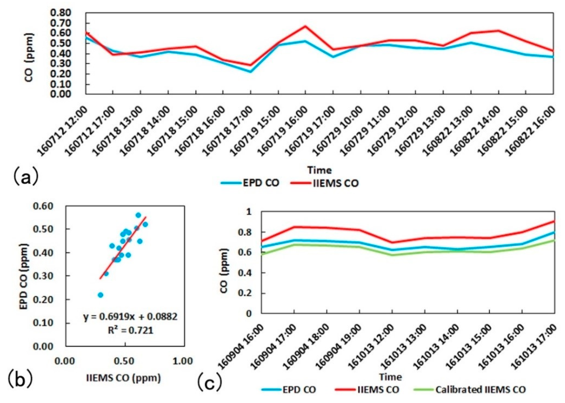
Figure 3.
Calibration results of SO2 data. (a) Comparison between EPD and IIEMS SO2 data; (b) Calibration curve for SO2; (c) Comparison of EPD, IIEMS, and calibrated IIEMS SO2 data.
Figure 3.
Calibration results of SO2 data. (a) Comparison between EPD and IIEMS SO2 data; (b) Calibration curve for SO2; (c) Comparison of EPD, IIEMS, and calibrated IIEMS SO2 data.
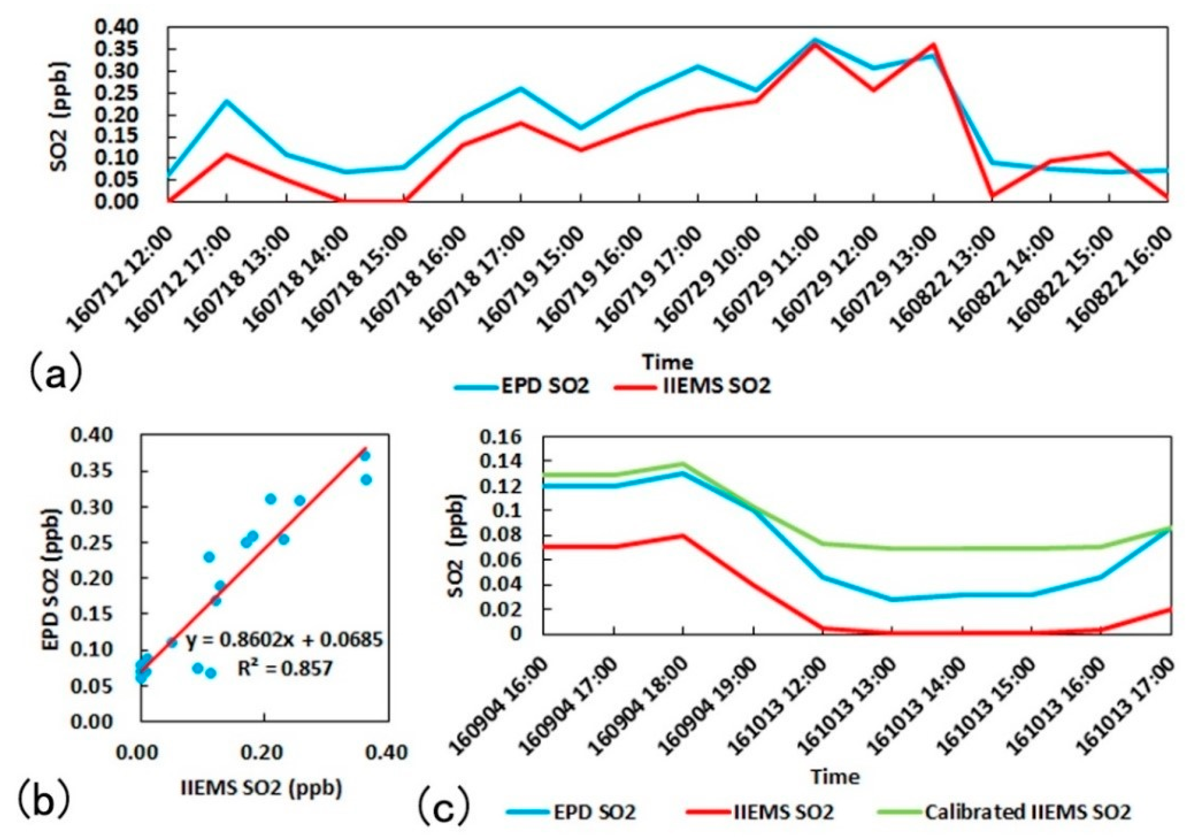
Figure 4.
Calibration results of particulate matter (PM) data. (a) Comparison between EPD and IIEMS PM10 and PM2.5 data; (b) Calibration curve for PM10 and PM2.5; (c) Comparison of EPD, IIEMS, and calibrated IIEMS PM10 and PM2.5 data.
Figure 4.
Calibration results of particulate matter (PM) data. (a) Comparison between EPD and IIEMS PM10 and PM2.5 data; (b) Calibration curve for PM10 and PM2.5; (c) Comparison of EPD, IIEMS, and calibrated IIEMS PM10 and PM2.5 data.
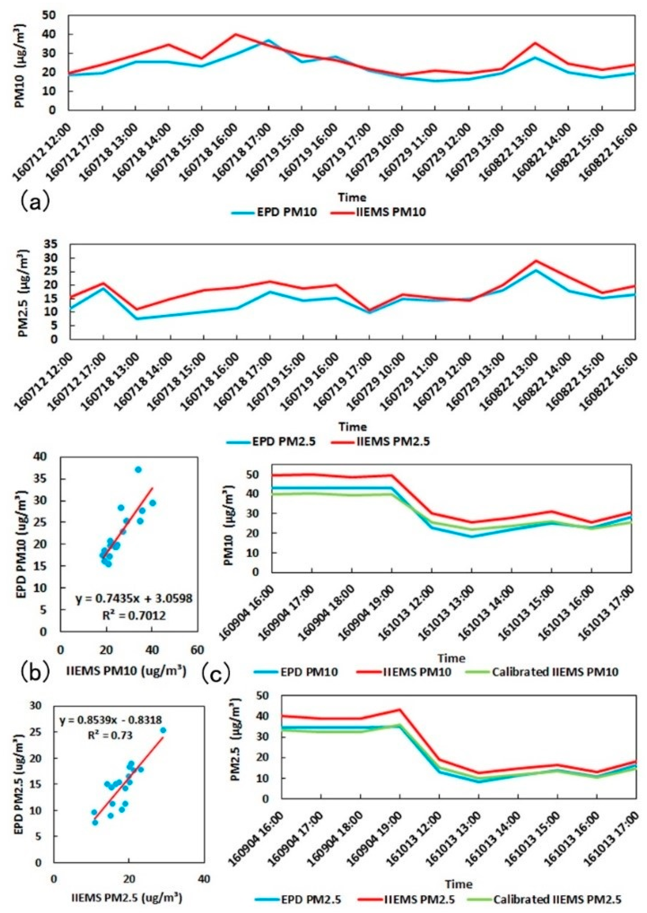
Figure 5.
Test results of all indices before and after Typhoon Nida along Nathan Road. (a) Comparison between temperature and humidity before and after Typhoon Nida; (b) Comparison between PM10 before and after Typhoon Nida; (c) Comparison between PM2.5 before and after Typhoon Nida; (d) Comparison between CO before and after Typhoon Nida; (e) Comparison between SO2 before and after Typhoon Nida; (f) Comparison between VOC before and after Typhoon Nida.

Figure 6.
Test results of all indices along Kowloon Park and Nathan Road. (a) Test result of temperature and humidity; (b) Test results of PM10 and PM2.5; (c) Test result of CO; (d) Test result of VOC; (e) Test result of noise.
Figure 6.
Test results of all indices along Kowloon Park and Nathan Road. (a) Test result of temperature and humidity; (b) Test results of PM10 and PM2.5; (c) Test result of CO; (d) Test result of VOC; (e) Test result of noise.


Table 1.
Specification of configuration scheme.
| Sensors | Relative Error | Range | Resolution |
|---|---|---|---|
| Temperature | ±0.3 °C | −25 °C–125 °C | 0.01 °C |
| Relative Humidity | ±1.8% | 0–100% | 0.03% |
| CO | ≤±2% FS | 0–500 ppm | ≤0.1 ppm |
| VOC (formaldehyde) | ≤±3% FS | 0–10 ppm | ≤0.01 ppm |
| SO2 | ≤±3% FS | 0–10 ppm | ≤0.05 ppm |
| Noise | ≤±0.5 dB | 30–120 dB | N/A |
| PM (PM2.5 and PM10) | <±15% | 0–999 μg/m³ | 1 μg/m³ |
| UV | ≤±3% FS | 0–10 | ≤0.1 |
Table 2.
Bold text indicates the best model with the lowest value of the Akaike information criterion (AIC).
Table 2.
Bold text indicates the best model with the lowest value of the Akaike information criterion (AIC).
| Variable | AIC—Typhoon Test | |||
|---|---|---|---|---|
| Model 1 | Model 2 | Model 3 | Model 4 | |
| CO | −1378.5 | −1551.4 | −1481.2 | −1558.7 |
| PM10 | 3771.6 | 2468.3 | 3738.0 | 2470.3 |
| PM2.5 | 3552.6 | 2253.3 | 3522.6 | 2257.1 |
| Temperature | 1242.5 | 367.0 | 484.7 | 254.2 |
| Humidity | 2555.9 | 1670.7 | 1803.9 | 1572.9 |
| SO2 | −1009.9 | −1039.7 | −1010.5 | −1036.1 |
| VOC | −2086.5 | −2232.7 | −2228.2 | −2261.5 |
| Noise | 3400.6 | 3338.2 | 3336.6 | 3327.6 |
| UV | −148.7 | −235.2 | −226.6 | −253.7 |
Bold text indicates the best model with the lowest value of the Akaike information criterion.
Table 3.
Estimated changes in environmental exposure after a typhoon event. Best models are the models determined by AIC based on Table 3 and are used to predict the environmental change after a typhoon.
Table 3.
Estimated changes in environmental exposure after a typhoon event. Best models are the models determined by AIC based on Table 3 and are used to predict the environmental change after a typhoon.
| Variable | Best Model | Difference between Days after a Typhoon and Days before a Typhoon (95% CIs) |
|---|---|---|
| CO (ppm) | Model 4 | 0.1 [0.05, 0.2] * |
| PM10 (μg/m³) | Model 2 | −0.8 [−4.4, 2.8] |
| PM2.5 (μg/m³) | Model 2 | −8.0 [−10.8, −5.2] * |
| Temperature (°C) | Model 4 | −0.7 [−1.2, −0.3] * |
| Humidity (%) | Model 4 | 5.9 [4.3, 7.4] * |
| SO2 (ppm) | Model 2 | −0.1 [−0.2, 0.008] |
| VOC (ppm) | Model 4 | −0.05 [−0.08, −0.02] * |
| Noise (db) | Model 4 | 6.6 [−2.5, 15.7] |
| UV (UV Index) | Model 4 | 0.7 [0.5, 1.0] * |
* Indicates significant results.
Table 4.
Bold text indicates the best model with the lowest value of AIC.
| Variable | AIC—Kowloon Park Test | |||
|---|---|---|---|---|
| Model 1 | Model 2 | Model 3 | Model 4 | |
| CO | −409.8 | −445.6 | −420.0 | −445.2 |
| PM10 | 812.3 | 468.3 | 802.14 | 468.3 |
| PM2.5 | 786.2 | 443.5 | 774.1 | 442.2 |
| Temperature | 243.3 | −55.8 | 116.8 | −63.6 |
| Humidity | 629.4 | 336.1 | 515.3 | 337.1 |
| VOC | −600.2 | −601.6 | −602.4 | −610.0 |
| Sound | 866.8 | 863.2 | 861.9 | 863.2 |
| UV | 492.1 | 485.2 | 475.8 | 464.6 |
Table 5.
Estimated change in environmental exposure on an urban road. Best models are the models determined by AIC based on Table 5 and were used to predict the environmental change on the urban road. * Indicates significant results.
Table 5.
Estimated change in environmental exposure on an urban road. Best models are the models determined by AIC based on Table 5 and were used to predict the environmental change on the urban road. * Indicates significant results.
| Variable | Best Model | Difference between Road and Park (95% CIs) |
|---|---|---|
| CO (ppm) | Model 2 | −0.02 [−0.08, 0.03] |
| PM10 (μg/m³) | Model 2 | −0.4 [−1.9, 1.2] |
| PM2.5 (μg/m³) | Model 4 | 0.1 [−1.3, 1.6] |
| Temperature (°C) | Model 4 | 0.5 [0.3, 0.7] * |
| Humidity (%) | Model 2 | 0.8 [−0.1, 1.7] |
| VOC (ppm) | Model 4 | −0.01 [−0.04, 0.02] |
| Noise (db) | Model 3 | 8.0 [2.5, 13.6] * |
| UV (UV Index) | Model 4 | −0.9 [−2.4, 0.7] |
© 2018 by the authors. Licensee MDPI, Basel, Switzerland. This article is an open access article distributed under the terms and conditions of the Creative Commons Attribution (CC BY) license (http://creativecommons.org/licenses/by/4.0/).
Share and Cite
MDPI and ACS Style
Wong, M.S.; Wang, T.; Ho, H.C.; Kwok, C.Y.T.; Lu, K.; Abbas, S. Towards a Smart City: Development and Application of an Improved Integrated Environmental Monitoring System. Sustainability 2018, 10, 623. https://doi.org/10.3390/su10030623
AMA Style
Wong MS, Wang T, Ho HC, Kwok CYT, Lu K, Abbas S. Towards a Smart City: Development and Application of an Improved Integrated Environmental Monitoring System. Sustainability. 2018; 10(3):623. https://doi.org/10.3390/su10030623
Chicago/Turabian StyleWong, Man Sing, Tingneng Wang, Hung Chak Ho, Coco Y. T. Kwok, Keru Lu, and Sawaid Abbas. 2018. "Towards a Smart City: Development and Application of an Improved Integrated Environmental Monitoring System" Sustainability 10, no. 3: 623. https://doi.org/10.3390/su10030623
Note that from the first issue of 2016, this journal uses article numbers instead of page numbers. See further details here.