The Consumer Demand Estimating and Purchasing Strategies Optimizing of FMCG Retailers Based on Geographic Methods

1
State Key Lab for Information Engineering in Surveying, Mapping and Remote Sensing, Wuhan University, 129 Luoyu Road, Wuhan 430079, China
2
Collaborative Innovation Center of Geospatial Technology, Wuhan University, Wuhan 430079, China
*
Author to whom correspondence should be addressed.
Sustainability 2018, 10(2), 466; https://doi.org/10.3390/su10020466
Submission received: 27 December 2017
/
Revised: 7 February 2018
/
Accepted: 8 February 2018
/
Published: 9 February 2018
(This article belongs to the Section Economic and Business Aspects of Sustainability)
Abstract
:The fast-moving consumer goods (FMCG) industry is expected to grow dramatically given the rapid increase in purchasing power of Chinese consumers over recent years. In order to facilitate the sustainable development of the Chinese FMCG market, it is important for FMCG retailers to understand the provincial market demand and make out flexible purchasing strategies. This paper proposes a new combination of geographic methods to estimate market demand at the micro-scale through historical sales data. Based on the consumer demand of regions and the sales performance of nearby regions, this study also proposes a method to decide what kinds of optimizing purchasing strategies should be adopted for the retailers in different areas, the positive strategies or the conservative strategies. The sales data of FMCG retailers in Guiyang was used in the experiment, and the results showed that their theoretical sales could be improved by over 6.5% and 10.2 under two strategies. The findings indicate that this study can provide practical guidance for retailers to estimate the market demand, and develop suitable optimizing purchasing strategies, thus improving the profit of retails and decreasing the risk of products waste.
1. Introduction
The concept of sustainable development requires us to allocate resources in the most appropriate way to satisfy the demand of our society. The estimating of market demand is recognized as the most important concerns in many business domains, such as the electric power industry [1], perishable food industry [2], and the housing market [3].
Given the continuous growth of the Chinese economy, the Fast Moving Consumer Goods (FMCG) industry in China is becoming one of the largest markets in the world [4]. To retailers and malls, increasing demand for FMCG may bring higher profits. However, Chinese consumption behaviors have undergone tremendous changes, and the regional characteristics of the FMCGs consumers are becoming increasingly complex [5]. The unreasonable purchasing strategies of FMCG retailers often cause waste and loss in some places, and shortage in other places, thereby bringing out negative impact on the sustainability of economics [6,7,8]. That indicates the need for appropriate forecasting of consumer demand, thus the quantity of products that retailers should prepare, and is a main challenge for the sustainable development of FMCG market [9].
In European supermarkets, the FMCG attrition rate can reach 15–20%, which may block the development of a sustainable economy and lead to losses amounting to millions of dollars [10,11]. To reduce profit loss, some retailers will set a higher price for FMCGs, thereby leading to the decrease of consumer purchasing frequency [12]. As estimating market demand is a critical part of supply chain management, the problem of predicting stock levels can also result in significant problems for the manufacturers that fill orders from retailers [13]. The manufacturer cannot truly obtain the right consumer information to guide their production. The relevant knowledge of consumer preferences and demand assists the conduct of future economic strategies of both the manufacturer and retailer [14].
To estimate the market demand and make out better business strategies, Anderson [15] tried to collect preference data of consumers through surveys and questionnaires, and found out the most popular goods and the characteristics of target consumers. The questionnaire survey is the most straightforward way to get consumer information, however, it is also labor-intensive and time-consuming, thus leading to the limited quantity of respondents [16,17]. Later on, some time series methods are used to predict the future sales based on the historical data. Chien [18] used the Moving Average (ARIMA) method and Grey neural network approach to predict the consumer demand of the whole area based on the historical sales data. Iva [19] used the ARIMA model to predict the tourism development of Montenegro in the next 5 years. Mustafa [20] used the SARIMA model to forecast the demand of energies. As the time series methods were often used for the prediction of the market demand in a whole city or province, the results were useful for some industries like cars industry and electric industry to conduct the total distribution strategies between cities. To single retail shop or supermarket, however, the time series analysis results of a whole city could not provide practical purchasing strategies for them. Instead, more detailed factors should be take account. For example, the consumer demand in the city centers was often different from that in suburban areas, which would lead to different sales performance to the retail shops located in different areas [21]. In this way, the locations and spatial factors should be taken account to guide the purchasing strategies of small retail shops.
In order to get more information of the local consumer demand, some researchers used geographic approaches to explore the distribution patterns of retailers. Elliot [21] used the kernel density estimation to estimate the commercial centers of sports retailers, and found out there existed three consumer patterns in study city, which indicated the consumer demand was different in the commercial centers and other places. Many studies use different theories, such as central place theory [22], kernel density estimation [23], and distance attenuation theory [24]. These theories are often used to estimate the commercial centers of retailers or malls, combining sales data with external data such as media or POI data [25]. Given limited data sources, current studies cannot detailly make analysis of the quantity and distribution of retailers [26], and explore their spatial characteristics. According to the Tobler’s “first law of geography”, there exists a similarity and connectivity between the nearby geographic units [27]. In the work of Zheng [28], the spatial dependencies were found existed between nearby geographic units. Because of the mobility of people, the inflow of a region was affected by the outflow of nearby regions, and would be the inflow of other regions in the next time period [28]. His work indicated that, different from the unmoved POI, the population in a region would also affect the floating population in its nearby regions, thus affecting the traffic, commercial and other domains.
Our novel contribution is that we introduce a method to estimate the consumer demand in micro-scale like geographic grid cells and take out optimizing purchasing strategies according to the spatial auto-correlation of consumer demand of nearby grids. The method was applied to the 5614 FMCG retailers in Guiyang City. The results showed that our method could effectively estimate the consumer demand and help retailers devise purchasing strategies.
The paper is organized as follows: in Section 2, we review related studies on the study of consumer demand and the purchasing strategies. In Section 3, we introduce the methodology used in the research. In Section 4, clustering analysis of FMCG retailers in Guiyang is conducted to find the consumer demand of the whole areas. In Section 5, the consumer demand in micro-scale is estimated and optimizing purchasing strategies are put out. The conclusions and directions for future work are provided in Section 6.
2. Literature Review
In the traditional methods, the consumer demand was predicted just through the historical dales data by using the methods like Moving Average (ARIMA) method and Grey neural network approach [18]. The methods were often used to predict the sales performance in a whole city or province, the results were useful for some industries like cars industry and electric industry to conduct the total distribution strategies. As to single retail shop or supermarket, more detailed factors should be take account. These methods ignored the spatial unevenness and patterns inherent in sales data, thus cannot adequately reflect consumer patterns and behaviors, which might lead to the loss of market share and inappropriate marketing strategy for retailers doing business in the Chinese marketplace. So that consumer preferences were needed for retailers to adjust their marketing strategies in a timely manner, which could definitely improve sales. However, the preferences or characteristics of consumers are always difficult to obtain due to privacy concerns. An effective way was to collect preference data through surveys and questionnaires to estimate the consumer demand and decide which kinds of products to purchase [15]. The problem was that the data volume through the questionnaires was always small, thus cannot truly guide the distribution strategies of retailers in a large area. In order to solve this problem and obtain more consumer data, some researchers have used big social media data from Sino Wei-bo, the popular micro-bog platform in China. In their studies, the sign-in data was obtained through the Wei-bo API (Application Program Interface), and spatial clustered was conducted to find the hot sigh-in areas and the consumers in that places. They used the preference information of a small number of consumers through questionnaire survey to estimate the consumer demand of all hot areas. However, the social media data could not reflect the preference discrepancy between different areas. Moreover, the sign-in data was distributed mainly around the commercial centers or companies, and the data lacked the location information of retailers. That means the analysis through social media data cannot reflect the complex relationships between retailers, like competition and promotion relationships, and do not take consider of the number of retailers, so that these researches cannot put out practical optimizing strategies.
Retail sales data must be considered spatially, and incorporate a geographical perspective as consumer habits are closely related to location. By studying the spatial distribution of retail sales variations in consumer preferences over space can be effectively revealed, thereby helping businesses develop suitable marketing strategies and higher profits. Many fast fashion brands have been adopting geographical strategies to guide their product distribution, companies like Zara, which analyzed the different preferences in quality and style in different countries [29,30]. These analyses considered the total supply or sales performance of different countries; findings would guide production strategies and identify hot items for a country or province. The service areas of single retail shops, however, are usually several streets or blocks, the consumer demand analysis of whole city cannot truly guide their purchasing strategies. For small retail shops, the purchasing strategies should be adjusted according to nearby consumer demand rather than that of a whole city. Even when each retail shop sales the same hot item, the number of units of a hot item to buy still remain an art not a science. Retailers have to obtain the highest profit, within their cost constraints. Research on means to effectively extract the consumer characteristics at micro-scale, providing microscopic guidance for retailers is relatively lacking.
According to the Tobler’s first law of geography,” things closer together are more alike than things farther away” [27]. Based on this idea, a new combination of geographic methods is proposed to solve the problem of the distribution and sales strategies of FMCG among retailers. In this research, a method to estimate the consumer demand in micro-scale like geographic grid cells is introduced, and we take out pointed optimizing purchasing strategies according to the stability of consumer demand in different regions. The research can provide microscopic guidance for the development of a sustainable economy.
3. Methods
3.1. Clustering Algorithms
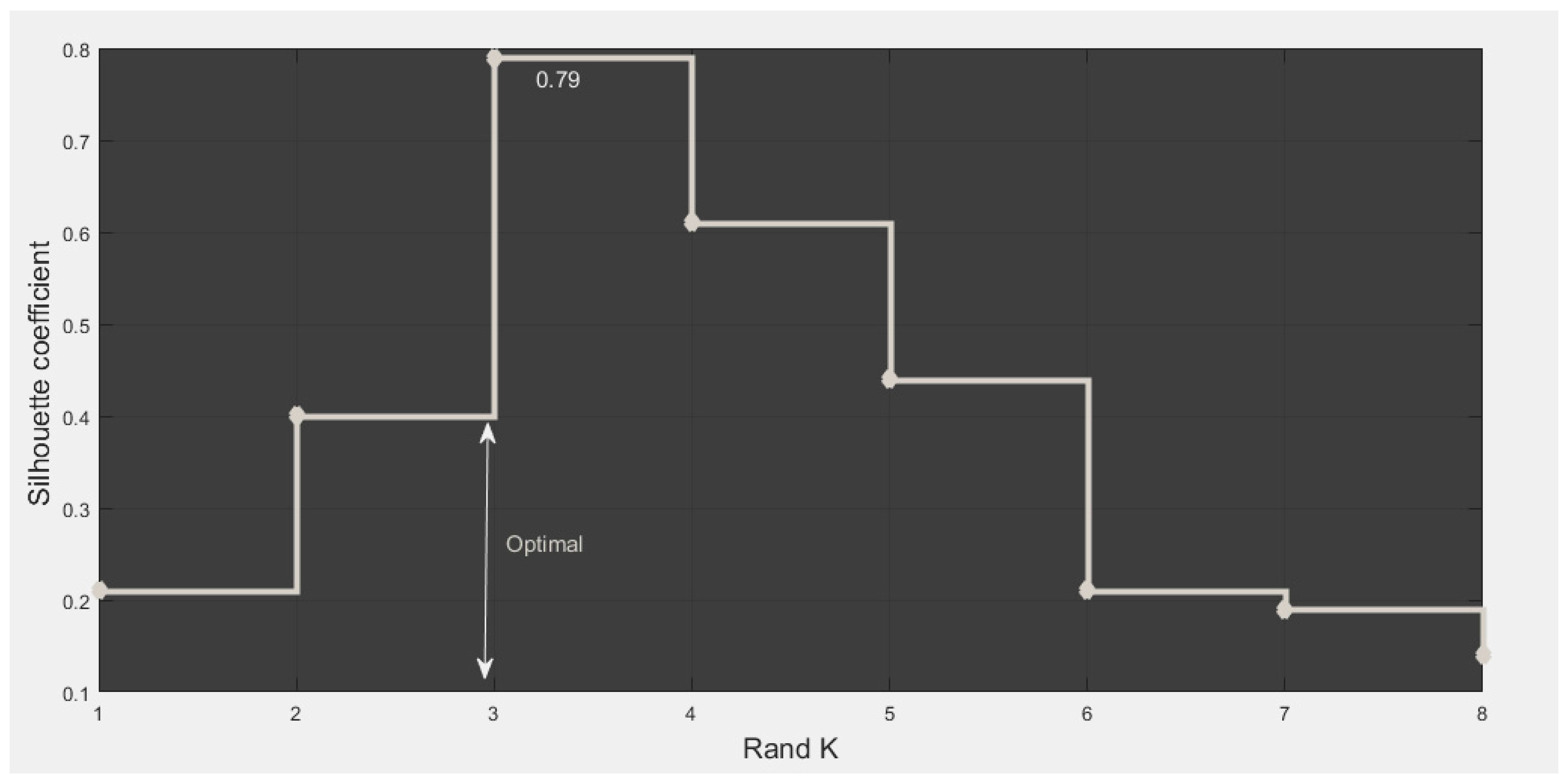
Clustering algorithms efficiently separate a data set, and aggregate data into several classes based on their characteristics [31]. Clustering algorithms are well-represented data mining, such as density-based spatial clustering of applications with noise (DBSCAN), Expectation-Maximization (EM), and K-means clustering algorithms [32]. Clustering algorithms have different advantages and weakness. DBSCAN is a method that considers the density of objects in certain areas; performing efficiently on data with significant noise. When the counts of these clustered objects are uncertain, such as the trajectory objects found in high-dimensional data, the quality of clustering algorithms may be compromised. K-means clustering algorithms, as distance clustering algorithms, take the distance of objects as a basic clustering reference, achieving effective and efficient performance on high-dimensional data [33]. In a K-means algorithm, the number of clusters K is set before implementing the algorithm; the silhouette coefficient can be used to evaluate different K values [34]. In our research, we evaluate silhouette coefficient with k value ranging from 2 to 8; the best K (3) was chosen as our cluster number.
To evaluate the accuracy of clustering, we used the KNN (K-Nearest Neighbor) classification algorithm to evaluate the accuracy of clustering results as classified by the clustering centers calculated by the K-Means algorithm [35]. KNN can determine the categories of sample data using only the classification of a few nearest objects [36]. We selected the sales data of 3/4 retail shops as the training data and the sales data of 1/4 retail shops was reserved as test data. In the training process, we use the half off cross validation method to construct the classifier of the training process. KNN delivers more effective performance than other methods, since the distribution of shops is nearly centralized, and the data set of shops includes elements with crossing or overlapping domains. Hence, we used the KNN algorithm for reclassification based on the cluster centers provided by K-means as well as in a comparison with the K-Means clustering results.
3.2. Spatial Autocorrelation
Spatial auto-correlation is the foundation for spatial statistical analysis; permitting the quantification, measurement, and evaluation of location and place-based effects on other phenomena like sales. Spatial auto-correlation can be used to estimate the similarity of attributes of different areas using global indicators, such as Moran’s I, Geary’s C, and Getis’s G [37,38,39]. To measure how sales are spatially auto-correlated among retailers in Guiyang, we used global Moran’s I values to assess the similarity of sales characteristics of retailers in nearby grid cells. Two strategies for improving sales were inferred from the spatial auto-correlation results. The value of Moran’s I always falls between −1 and 1. If the value is close to −1, that indicates the shops with high sales are surrounded shops with low sales. In contrast, when the value is close to 1, shops with high sales are surrounded by other shops with high sales. If the values are close to 0, then the sales of shops are random with no spatial effect on sales. In spatial auto-correlation analysis, a spatial weight matrix “” describes the spatial relationship between different areas [40], thus spatial weights tare assigned to pairs of units i and j. A row-standardized spatial weight matrix “” describes the neighbor relationships in spatial auto-correlation analysis, and subsequently, the matrix “” represents the spatial weights that are assigned to pairs of units i and j. The formulas of global Moran’s I and local Moran’s I are as follows [41]:
where n represents the total number of spatial units, the values of each unit are represented by “” or “”, and “” is the average value of all units. The matrix “” is the spatial weight that represents the spatial relationship between all areal units. To test the statistical significance of the observed Moran’s I, a Z value is calculated:
where and are their theoretically expected value and variance, respectively. If the calculated local Moran’s I is greater than expected, it indicates places within the data set with positive local spatial auto-correlation. If the local Moran’s I value is less than the expected value; then, places within the data set exhibit negative spatial auto-correlation. In an analysis of spatial auto-correlation, a “hot region” usually represents places that are close to each other and all possess relatively high Moran’s I values.
3.3. Spatial Division
Given that the marketing characteristics of retail shops are often regional, we can make adjustments to the distribution optimization strategy based on the regional characteristics of shops. Several methods for space division are available, including spatially weighted Voronoi diagrams, which can set sales as an attribute (weights) in spatial segmentation, and Delaunay triangulation. These two methods can take account of the differences between shops, but they cannot reflect the relationship between the retail shops. Compared to these two methods, the grid diagrams occupies several advantages [42,43], they are also very simple and easy to overlay.
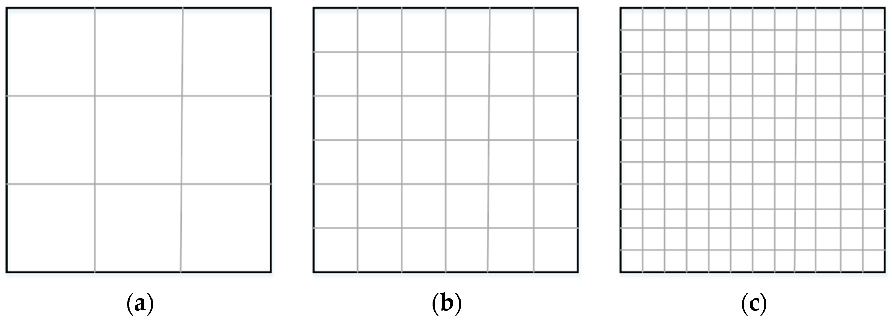
For class 1 shops, sales were relatively high, and their trade areas were broader. Thus, the grid size of the first class shops was set as 300 × 300 m, following the work of Yue [44]. For class 2 shops with relatively smaller service areas, we set a smaller grid size. A series of grid sizes between 30 × 30 m and 200 × 200 m were chosen, and the of each size was calculated, respective. The represents the fitting results between purchasing strategies and sales performance in each grid, and more details of will be introduced in the next section. Finally, the 150 × 150 m was set as the grid size of class 2 shops, with the highest value. The same method was used to class 3 shops, and the grid size of class 3 shops was set as 150 × 150 m.
The calculation method of each layer is similar. Thus, the first class of grid was chosen to calculate as an example. We set i to represent the grid number of level 1. Then, for grid i, we calculated the mean variance of and mean sales P of shops located in grid i. The grids for each class of shop are shown in Figure 1.
4. Date source and Cluster Analysis
4.1. Data Source
The main data set used in this paper is the location and monthly sales data of FMCG between 2015 and 2016 of the 5614 FMCG retail shops in Guiyang City, China. The data was provided by a local company. These shops include supermarkets and small stores. The FMCG in these shops included fresh foods like meat and vegetable, and frozen foods, wine, hygiene products and so on. We choose three types of FMCGs as our research objects. Other data set includes the road network and maps of Guiyang City as spatial references and a base map. The sales situation of 5614 FMCG retailers existed great differences, thereby the clustering analysis was used to classify the retailers and find different consumption patterns.
4.2. Market Segmentation by Cluster Analysis
In the study of market segmentation, a cluster analysis is usually applied to obtain the sales characteristics of different shops. The aim in data clustering is to group spatial data or multidimensional attribute data into several collections of clusters, and make the gap between different clusters as large as possible. In contrast, the differences between elements within the same class must be as small as possible [45]. The commonly used clustering algorithms include DBSCAN clustering algorithm and K-means clustering algorithm. The categories of retail shops are usually diverse; thus, the K-Means algorithm will yield higher accuracy compared to DBSCAN algorithm with this high dimensional shop data. Therefore, in this paper, we used K-Means clustering algorithm as the clustering method.
The classic K-Means clustering algorithm is based on distance; the algorithm uses the space between the object distances to evaluate the degree of aggregation between objects in the data set. This distance might not be spatial distance but a distance measurement representing other attributes, such as retail sales that could distinguish between objects such as stores in a data set [46]. The algorithm requires an appropriate clustering number, for the initial cluster centers in an iterative process. Thus, the distance of all samples to the inner centers are obtained and merged into the nearest cluster center, forming the initial clusters. The new cluster centers are calculated from initial clusters V(v1, v2, v3...), which are the core of initial clusters, and usually different from initial cluster centers. Through the new cluster centers, the sample data can form new clusters and cluster centers again, through this constant iterative updating, the data are clustered, until no new changes occur or are less than a threshold. In this way we obtained the final clustering centers and KNN classification results [47].
We selected three products that were represented by α, β and δ as the clustering objects. The sales of 5614 retail shops are apparently different. Only by classifying the shops by their sales of FMCG into several classes could we develop a pointed marketing program for every type of retail shop. To confirm the optimal number of clusters, the silhouette coefficient was introduced. It is a type of evaluation method that is used to estimate the consequences of clustering using a quantitative value ranging between −1 and 1. The method was proposed by Peter J. Rousseeuw in 1986 [48]. It can be used to the represent the similarity between the internal clusters and the degree of separation between different clusters. For an N-point data set, the method for calculating the contour coefficient is as follows:
where, a(i) represents the average distance of vector i to other points in its cluster, and b(i) represents the average distance of vector i to points of other clusters. The cluster number was set for 2 through 8, the K-Means clustering was conducted for each number. The results in Figure 2 show the changing of silhouette coefficient with different K values.
Figure 2 shows that when K = 3, the silhouette coefficient is highest, so we choose 3 as the clustering number to better distinguish retail shops. We used K-means clustering analysis to divide the whole 5614 retails into 3 clusters based on the sales of each kinds of goods. The clustering results are shown in Figure 3.
Green dots in the figure represent shops of that sell the three types of goods, sales are high. The red dots represent the shops whose sales are general, and the blue points represent shops with fewer sales. We calculated the clustering center of each type of shop and calculated the logarithm of clustering centers to weaken the gap between different magnitudes and make the divergent points more compact. To avoid the influence of shop sales abnormities and to obtain the general characteristics of shops, we used a random sampling method for multiple clustering. We randomly selected 80% of stores for clustering. Thus, we obtained a group of different cluster centers. We summarized the distribution of the cluster centers, presented in Table 1:
Table 1 shows shops are divided into three classes and that each class contains a clustering center of the goods of α, β, and δ. Class 1 represents the shops with high sales, in which the ratio of three products is (148.65, 114.36, 148.83). This kind of shop may be a supermarket or a big mall. The ratio may reflect the typical characteristics of this kind of shop. The table shows that the sales of α are nearly the same as δ. The sales of β are 66% of α and δ. Class 2 represents the shops with middle range sales. The ratio of three products is (62.79, 34.71, 78.76). In this kind of shops, product δ is sold more than α. The sales of β are about a half of α. Class 3 comprises small shops, and their sales are typically less than the other classes of shops.
4.3. Relationship between Sales and Cluster Centers
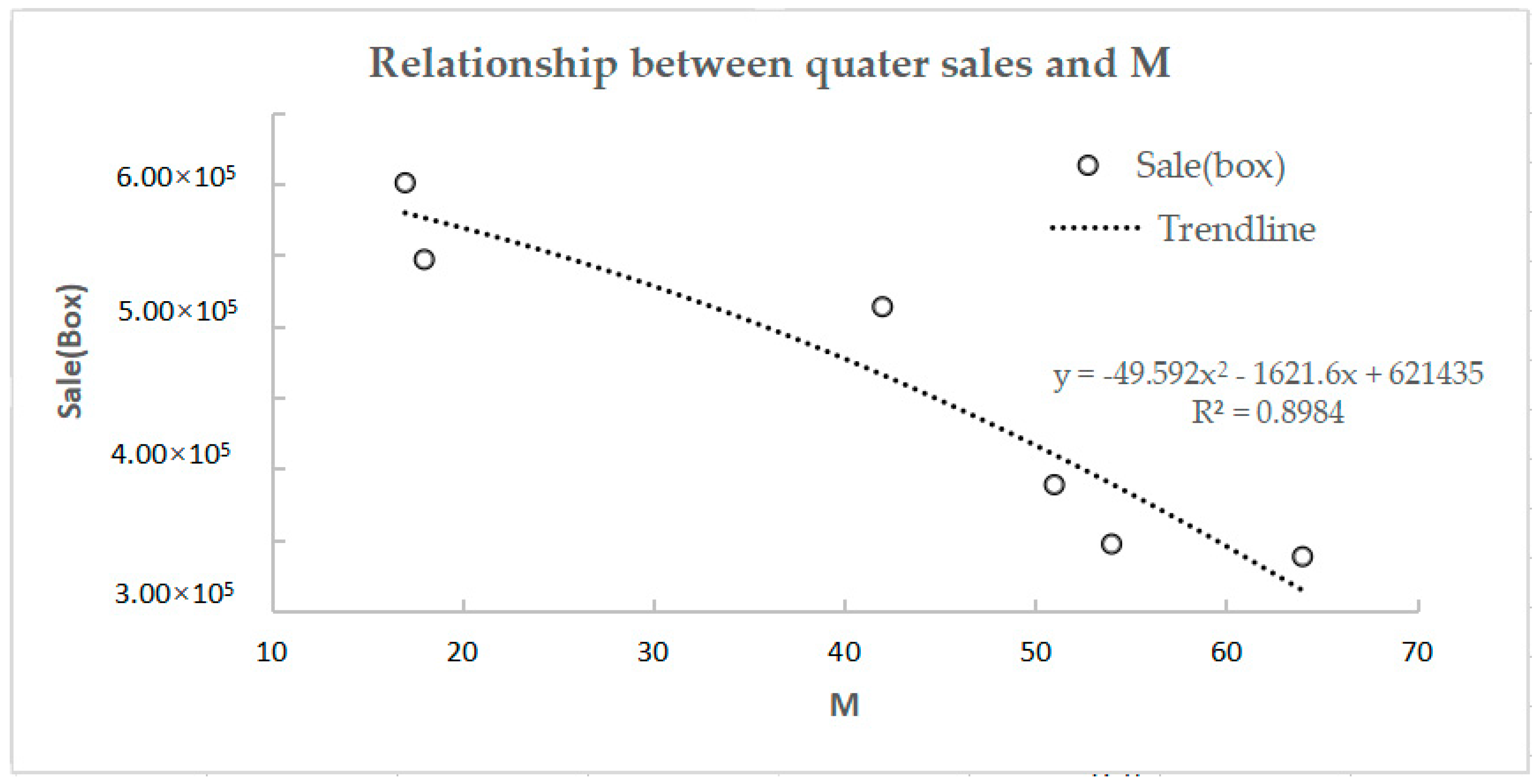
The cluster centers calculated above indicate characteristics of different types of shops, which can indirectly reflect consumer demand. The cluster centers could reflect different needs for FMCGs. Thus, how can we use this principle to satisfy consumer demand and promote the profit of shops at the same time? To find the relationship between shop sales and the ratio of FMCGs, we used the MLE (maximum likelihood estimation) method to estimate the optimal fitting function between shop sales and a variable called M. M is the variance of quarterly cluster centers and the standard deviation as calculated. The computational formula of M is as follows:
We calculated the cluster centers of every quarter and calculated M(i) for each month from 2015 to 2016 for the retailer shops. We used the maximum likelihood estimation method to find the relationship between M(i) and sales within each cluster; the original data was the monthly sales data, by stores. During data processing however, some retailers did not have the sales records for some products during certain months due to shortages of goods. We calculated the quarterly sales of each retail store using monthly sales data to reduce the impact of shortage conditions. The clustering results reflect consumer demand, so we used ordinary least squares regression to explore whether or not the quarters with high sales results had a better fit with the clustering centers. The M value was set as the independent variable to represent the gap between quarterly clustering centers and the total clustering centers as calculated. The quarterly sales values were set as the dependent variable.
To evaluate the fitting degree of the equation, we introduce the goodness of fit concept, which is based on the similarity between predicted values and the actual value [49]. The fitting statistics used in this paper is . The greater the , the closer their relationship [50]. Table 2 shows the fitting results.
The results from Table 2 clearly shows that high correlation occurs between shop sales and their quarterly M value, which is much better than the monthly M value, and the can reach 0.8858. The results are shown in Figure 4, as follows:
Thus, if the shops want to improve their theoretical sales, they must adjust their current quarterly distribution strategy to move closer to the standard clustering centers which better fit the consumer demand. The clustering center essentially reveals the population and acceptance for the retail brand of products. For each class of shop, if we take measures to move close to the cluster centers ratio, this approach will satisfy consumer needs and fit the market demand. These line fitting results will provide a guide for the improvement of sales while avoiding sales busts, at the same time. The results can reflect the market demand of the whole area. When the M value equals to 0, then the predicted largest market potential could be about 676,718 (boxes) through the formula. However, the demand potential maybe large in some places but small in the others, so that the spatial characteristics of consumer demand should be considered. To provide more practical guidance for the business of retailers, in the next section we will estimate the market demand in the more microcosmic scale, based on the results in this section, and take out targeted purchasing strategies for each area.
5. Consumer Demand Estimating and Purchasing Strategies Optimizing
5.1. Estimating Consumer Demand in Grids
Realistically, to increase profits, the distribution ratio must be maintained near the cluster centers from the results in Section 3. The implementation of the principle however, is the main problem for retail shops, because the actual market demand exists great differences between areas or even nearby streets. For each store, their current distribution and ratio of products are different from the standard clustering center X (X1, X2, and X3). The difference may be small for some shops but may be large for other shops. If we blindly adjust the distribution strategy for every shop and dramatically shrunk the gap between the current ratio and standard clustering center, then this approach will definitely cause a bust in the sales of products, thereby causing the risk of profit losses to the shops. Thus, the precise marketing strategy will be based on spatial auto correlation algorithm.
We took first class shops as experimental objects. The analysis of the other two classes of shops was similar. The 453 shops grouped in the first class were distributed in several areas of Guiyang. For every shop, there was variance M, describing the gap between its current ratio and the standardized ratio. We selected shops with small M values and large spatial aggregation values. We could decrease the gap between these shops to a large degree and decrease the gaps of shops whose M values were high by a small degree, by changing their distribution strategy.
Spatial correlation is an important research method in spatial statistical analysis; it is used to explore the degree of influence between regions. In spatial auto correlation analysis, a hot region usually occupies a place with relatively high values; retailers in hot regions are close to each other. However, in our data set, the M value of shops with high sales is relatively small. Thus, to satisfy the assumptions for auto correction analysis, we use a reciprocal variance to represent the gap between current products ratio and standard ratio. We use to represent the reciprocal variance; the formula is as follows, in which represents the average gap of the 6 quarters. The consumer demand in grid cells with large is higher than the grid cells with small :
We used spatial auto correlation analysis based on the of first-class shops. This result was then used to determine an appropriate distribution optimization strategy for each retail shop. We use two methods of analysis. First, we directly conducted spatial auto correlation analysis for shop points. Second, we conducted spatial auto correlation analysis based on the spatial segmentation model, in this case for grid cells.
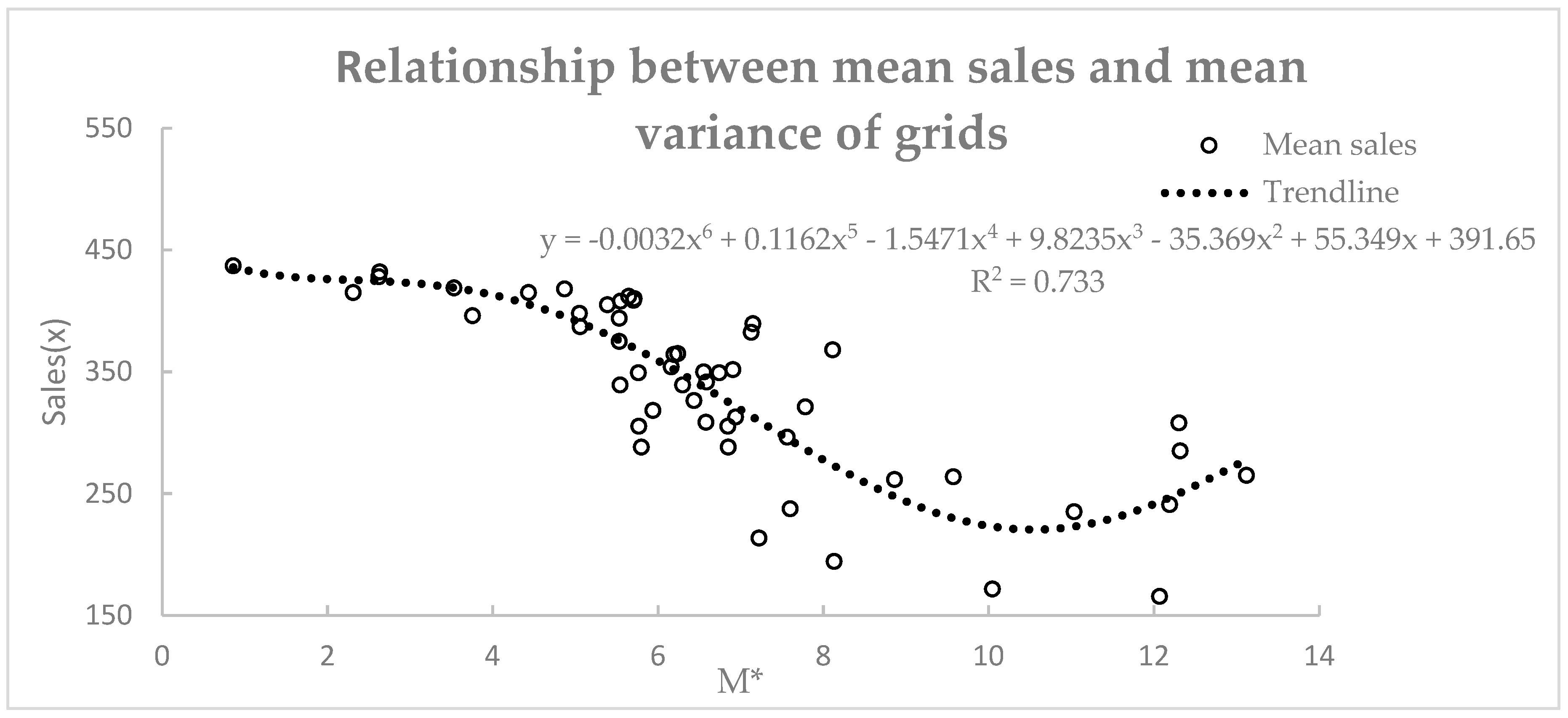
We created a scatter plot for and mean sales, based on which we established the functional relationship between the and mean sales using maximum likelihood estimation. The results are shown in Figure 5.
Figure 5 shows there exists high correlation between and sales in each grid cell, with the high R2 value 0.733. Table 3 shows the effects of the grid-based spatial division method we adopted. We compared the R2 calculated by the retailers and by grid cells.
Table 3 indicates that using the grid as a geographical unit is better than merely using single retailers, with lager R2. The sales model can provide support for planning the distribution strategies of shops that belong to the same grid. The model can also predict sales in each grid based on their variance.
Our goal is to improve the total sales by grid cells and adjust the distribution strategy of shops whose current sales situation is not favorable, thereby improving their profit and satisfying consumer demands at the same time. Our research provides an efficient method to do so. We used a spatial auto correlation method based on the of first-class grids to find out different patterns of market demand in different grids. Figure 6 shows the spatial auto correlation results for shops that belong to class 1.
Figure 6 shows the auto correction results, and the grids are distinguished into 3 colors. The red regions were areas in which market demand was “high–high” aggregations. The purchasing strategies of shops in these regions were generally close to the clustering center, indicating the consumer demand was relatively high and stable in these places. Thus, we can optimize the purchasing strategies of the shops located in these areas whose purchasing ratio does not match the market demand. This adjustment will bring their purchasing ratio closer to the clustering center. This approach will effectively improve their sales. For the retailers located in orange areas, the market demand is “high–low” or “low–high” aggregation, which means the market demand of nearby grids existed large difference with the grid. The market demand of the orange areas was lower than the red areas, but higher than the transparent areas. The distribution strategies of these shops can be adjusted slightly, and the focus can be on improving the shops whose values are below the average level in their grid. For retail shops located in the transparent grid, their market demand was ‘low–low’ aggregating or other situations. Thus, their statuses could be retained, or fine adjustments can be applied. Table 4 shows the shop numbers and average M* in grids of 3 colors.
From Table 4, we can see the shop number, value in the grid cells of three colors. There were 75 retailers in the red regions, and the average value of the retailers was 5.9.There were 141 retailers in the orange regions, the average value of the retailers was 8.6.There were 237 retailers in the Transparent regions, and the average value of the retailers was 12.1.The variety of values means the consumer demand exists differences to the retailers in the grids of 3 colors, which indicate that the optimizing strategies should be taken according to the differences of consumer demand.
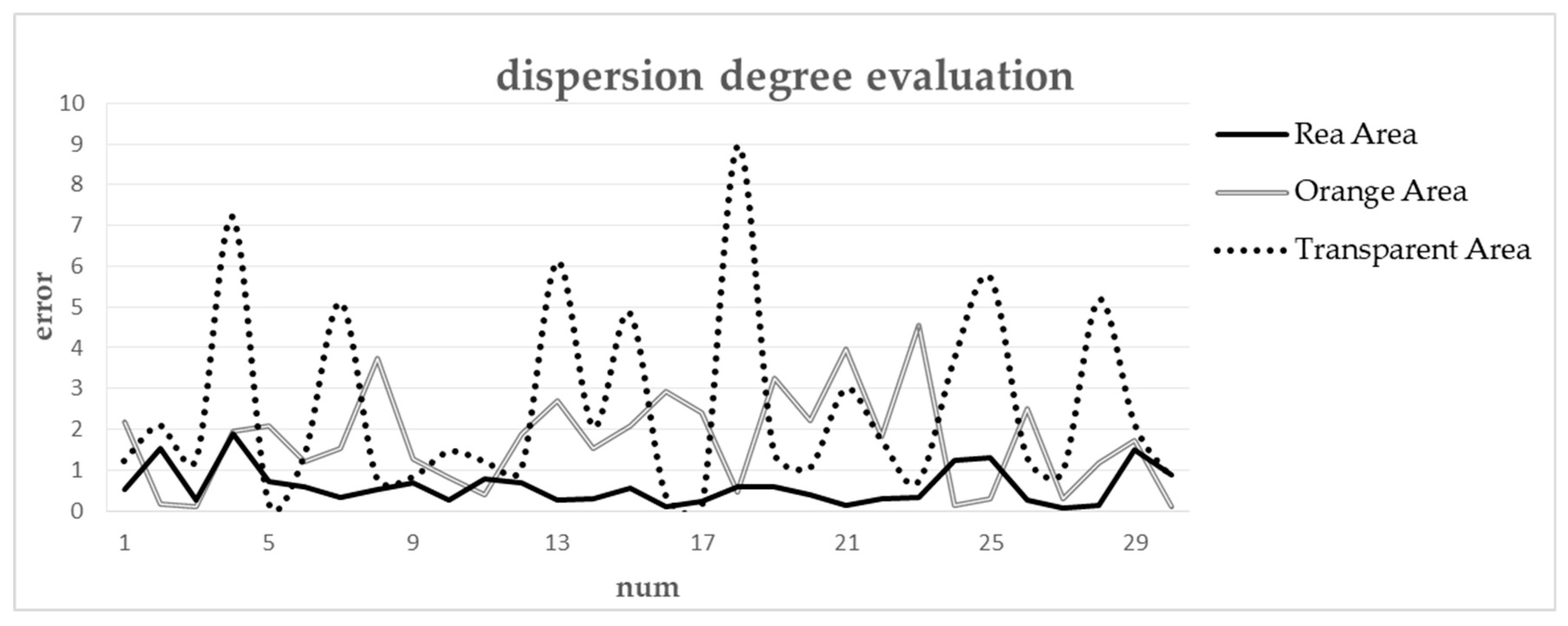
In order to verify if the grids can effectively reflect the consumer demand in different areas, we used Gauss test to find the sales situation in different colors of grids. We randomly chose 50 retailers in each color of grids, and used R studio to calculate the P-value of them, the results were shown in Figure 7.
The benefits of this method include two parts: Firstly, the consumer demand of each grid can be estimated with the , which will present more microscopic information of consumer demand for retailers. Secondly, the method can provide information about which kinds of adjustment strategies should be taken for retailers based on the colors of grids they belong to. That means not every retailer should adjust their purchasing strategies to the maximum market demand, the strategies should be considered according to their locations to avoid bust of sales, the thought of which a reflect of sustainable concept.
5.2. Optimized Purchasing Strategies
To obtain the sales situation in grids with different colors, we selected 10 shops in the red area and 10 shops in the orange area. We divided the shops into two groups according to their colors of grids. These two groups of retailers both belong to the First Class. The sales situation shown in Table 5.
Table 5 shows that the average sales of shops in group1 were larger than group2, while the values of shops in group1 were smaller than group2.This indicates that the consumer demand in group1 was larger than group2. In order to improve the regional sales and avoid sales bust, we need to adjust values in the right way.
In this paper, we implemented specific adjustments to purchasing strategies. The first was a positive strategy. The positive strategies were recommended to retail shops that satisfied two conditions. The first condition was the average sales of the region were very high. The second condition was that there existed high spatial autocorrelation between the sales of the region and its nearby regions. That indicated the consumer demand around these shops was relatively high and stable, so that the purchasing strategies of retail shops that did not sale well could be adjusted closer to the average level to get more profit. In this strategy, the values of the shops of Group1 below average value would be adjusted to the average value _1. The second strategy was a conservative strategy that could raise the value to _2, the average value of the current value for each shop and the average value of all retailers in group1. The conservative strategies were recommended to retail shops with middling sales performance and lower spatial autocorrelation between regions. These retail shops mainly distributed not far from the city centers. The main purpose of the strategy was to adjust the sales strategies based on their current sales performance. The strategies could ensure the stability of their sales performance, and bring small increase of profit for them. The _1 and _2 values are calculated as following:
Table 6 indicates the effect of these two strategies on sales. The predicted sales for each product was also calculated. The best percentage can be confirmed by the sales performance.
The Table 6 shows the influence of the two strategies on retailers in red areas and orange areas, respectively. For the 10 retailers in red regions with ID between G1.1 to G1.10, the sales situation was much better than the retailers in other regions with the average sales reaching 340, and the auto-correction of them were also relatively higher. That indicated that market demand of red regions was the highest among all regions, and the low average M* value 5.07 also indicated the stability of the market demand. Based on the above reasons, the positive strategy could be adopted to improve the sales of retailers in the red regions. The average M* value 5.07 was used to estimate the market demand quantity, which was 356, based on the formula in Table 3 (y = −0.0032x6 + 0.1162x5 − 1.5471x4 + 9.8235x3 − 35.369x2 + 55.349x + 391.65).
From Table 6, we can see 5 retail shops, G1.3 G1.4 G1.5 G1.7 G1.10, the original sales of which were lower than 340, were suggested to improve the purchasing quantity to 356. The best purchasing ratio of three products (128,100,128) was also calculated based on the clustering analysis results. Then, the purchasing strategies of the 5 retail shops was adjusted to 128,100,128, in this way, the theoretical average sales of shops in the red regions could reach 362, which was improved by 6.4%.
To the 10 retailers in orange regions with ID between G2.1 to G2.10, the sales situation was more worse than the red regions, but better that the transparent regions. The average sales of them were 182 and the average value of them was 8.8, which indicated the market demand of these regions was not very stable as the red regions. The regions might be some places nearby the commercial centers, to the shops in these places, the conservative strategies were adopted to improve the sales in these places and avoid the bust at the same time. There were 5 retail shops, G2.2 G2.3 G2.4 G2.6 G2.8, the sales of which were lower than the average sales, so that the values of them were adjusted to be the average value of their current value and 8.8. The purpose of the strategy was to adjust the sales strategies based on their current sales performance. The theoretical sales were estimated based on the new values, and the purchasing ratio of three products was also calculated. The theoretical average sales could reach 200, which was improved by 9.8%.
To retailers in transparent regions, the average value was 12.1, which was larger than the red and orange regions, so that the market demand in these regions was nearly small and not stable. In this paper, we think the adoption of new purchasing strategies may be meaningless even would cause some bust of sales in these places, so that the retailers in these regions just need to keep their current purchasing strategies.
In the practical business, other optimizing strategies can also be considered based on the strategies we put out in this section. For instance, the value of the retailers in red regions with higher sales can also be adjusted to be closer to 0 to reach the maximum potential of market demand, which was based on the purchasing ability of retailers. The most important thing is that all the adjustment should be based on the locations of retailers and sales performance of the region and nearby regions, which was represented with different colors in this paper. It is an effective way to carry out practical strategies for every retailer.
6. Conclusions
The concept of sustainable development requires us to allocate resources in the most appropriate way to satisfy the demand of our society. The estimating of market demand is recognized as one of the most important concerns in many business domains [51]. In our research, we introduced a method to estimate the consumer demand in micro-scale like geographic grid cells and take out pointed optimizing purchasing strategies according to the stability of consumer demand in different regions. The main works and contributions are as follows:
- (1)
- The research introduced a method to estimate the consumer demand in micro-scale, and verified that the purchasing ratio should be closer to consumer demand to get more profit. The estimate of the consumer demand was not only based on the sales performance of the current region but also considered the sales performance of nearby regions.
- (2)
- This research proposed a method for small retail shops to generate optimized purchasing strategies according to the consumer demand. The model we established could estimate the stability of consumer demand of different regions, and put out three different strategies including positive, conservative and remain unchanged strategies to the different regions. That will help the retail shops get more profit and reduce risk of loss.
- (3)
- The research conducted experiment with the actual sales data of 5614 FMCG retailers, which could be a representative example in the business field.
One important issue in the sustainable economic development is to avoid the loss of goods and get more profit [51]. The research can provide a grids-map of the city to retailers, and the grids will reflect the potential consumer demand and the best optimizing strategies, that will be helpful for retail shops to increase their profit and avoid the products waste at the same time. Furthermore, the research can provide information of the sustainable production. So that, the research will be beneficial for the development of sustainable economy.
In this context, the factors we toke considered were limited, and the retailers were just divided according to their sales. In future work, we will take account of more attributes of retailers like size and business circle, for a more precise analysis of consumer demand. Geographical attributes were not sufficiently considered in this research, furthering future work, we will incorporate more attributes such as road connectivity to each grid cell, for more accurate and precise results.
Acknowledgments
This research is supported by the National Natural Science Foundation of China (Grant 41471323). The author wishes to thank Wang Yankun, Li Chuanyong, Zeng Jia, Zhao Cheng, Yang Mei for helping to collect the data for the cognition experiments.
Author Contributions
Wang Luyao and Fan Hong conceived and designed the main idea and experiments; Wang Luyao and Gong Tianren performed the experiments; Wang Luyao wrote the paper.
Conflicts of Interest
The authors declare no conflict of interest.
References
- Venkatesan, N.; Solanki, J.; Solanki, S.K. Residential demand response model and impact on voltage profile and losses of an electric distribution network. Appl. Energy 2012, 96, 84–91. [Google Scholar] [CrossRef]
- Amorim, P.; Costa, A.M.; Almada-Lobo, B. Influence of consumer purchasing behaviour on the production planning of perishable food. OR Spectr. 2013, 36, 669–692. [Google Scholar] [CrossRef]
- Tsai, I.C. Housing affordability, self-occupancy housing demand and housing price dynamics. Habitat Int. 2013, 40, 73–81. [Google Scholar] [CrossRef]
- McNeill, L.S. The influence of culture on retail sales promotion use in chinese supermarkets. Australas. Mark. J. AMJ 2006, 14, 34–46. [Google Scholar] [CrossRef]
- Pan, S.L.; Ballot, E. Open tracing container repositioning simulation optimization: A case study of FMCG supply chain. Stud. Comput. Intell. 2015, 594, 281–291. [Google Scholar]
- Adrian, M.; Eliza, M.A.; Alexandru, C.; Costel, N. Design of a Customer-Centric Balanced Scorecard—Support for a Research on CRM Strategies of Romanian Companies from FMCG Sector. Available online: http://wseas.us/e-library/conferences/2010/Penang/MMF/MMF-19.pdf (accessed on 9 February 2018).
- Aitha, P.K.; Lagishetti, S.; Kumar, S.; Singh, A.; Nanda, A.K.; Shetty, S.; Vallala, S.; Pandey, R. Modeling production economies of scale in supply chain network design dss for a large FMCG firm. In Proceedings of the 4th International Conference on Operations and Supply Chain Management, Hongkong and Guangzhou, China, 25 July–31 July 2010. [Google Scholar]
- Ali, S.S.; Dubey, R. Redefining retailer’s satisfaction index: A case of FMCG market in india. Procedia Soc. Behav. Sci. 2014, 133, 279–290. [Google Scholar] [CrossRef]
- Islek, I.; Oguducu, S.G. A retail demand forecasting model based on data mining techniques. In Proceedings of the 2015 IEEE 24th International Symposium on Industrial Electronics (ISIE), Buzios, Brazil, 3–5 June 2015; pp. 55–60. [Google Scholar]
- Andriulo, S.; Elia, V.; Gnoni, M.G. Mobile self-checkout systems in the FMCG retail sector: A comparison analysis. Int. J. RF Technol. Res. Appl. 2015, 6, 207–224. [Google Scholar]
- Anselmsson, J.; Bondesson, N. Brand value chain in practise; The relationship between mindset and market performance metrics: A study of the swedish market for FMCG. J. Retail. Consum. Serv. 2015, 25, 58–70. [Google Scholar] [CrossRef]
- Chen, M.; Wakai, R.T.; Van Veen, B.D. Variance-based spatial filtering in FMCG. In Proceedings of the 22nd Annual International Conference of the IEEE Engineering in Medicine and Biology Society, Chicago, IL, USA, 23–28 July 2000; pp. 956–957. [Google Scholar]
- Ding, Q.; Dong, C.; Pan, Z. A hierarchical pricing decision process on a dual-channel problem with one manufacturer and one retailer. Int. J. Prod. Econ. 2016, 175, 197–212. [Google Scholar] [CrossRef]
- Kellner, F.; Otto, A.; Busch, A. Understanding the robustness of optimal FMCG distribution networks. Logist. Res. 2013, 6, 173–185. [Google Scholar] [CrossRef]
- Anderson, E.W.; Fornell, C.; Lehmann, D.R. Customer satisfaction, market share, and profitability: Findings from sweden. J. Mark. 1994, 58, 53–66. [Google Scholar] [CrossRef]
- O’Kelly, M.E. Trade-area models and choice-based samples: Methods. Environ. Plan. A 1999, 31, 613–627. [Google Scholar] [CrossRef]
- Lin, M.; Lucas, H.C.; Shmueli, G. Research commentary—Too big to fail: Large samples and the p-value problem. Inf. Syst. Res. 2013, 24, 906–917. [Google Scholar] [CrossRef]
- Chien, C.-F.; Chen, Y.-J.; Peng, J.-T. Manufacturing intelligence for semiconductor demand forecast based on technology diffusion and product life cycle. Int. J. Prod. Econ. 2010, 128, 496–509. [Google Scholar] [CrossRef]
- Bulatović, I.; Stranjančević, A.; Lacmanović, D.; Raspor, A. Casino business in the context of tourism development (case: Montenegro). Soc. Sci. 2017, 6, 146. [Google Scholar] [CrossRef]
- Akpinar, M.; Yumusak, N. Year ahead demand forecast of city natural gas using seasonal time series methods. Energies 2016, 9, 727. [Google Scholar] [CrossRef]
- Rabinovich, E.; Rungtusanatham, M.; Laseter, T.M. Physical distribution service performance and internet retailer margins: The drop-shipping context. J. Oper. Manag. 2008, 26, 767–780. [Google Scholar] [CrossRef]
- Oppewal, H.; Holyoake, B. Bundling and retail agglomeration effects on shopping behavior. J. Retail. Consum. Serv. 2004, 11, 61–74. [Google Scholar] [CrossRef]
- Silverman, B. Density estimation for statistics and data analysis. Chapman Hall 1986, 37, 1–22. [Google Scholar]
- Huff, D.L. Defining and estimating a trading area. J. Mark. 1964, 28, 34–38. [Google Scholar] [CrossRef]
- Paralikas, J.; Fysikopoulos, A.; Pandremenos, J.; Chryssolouris, G. Product modularity and assembly systems: An automotive case study. CIRP Ann. Manuf. Technol. 2011, 60, 165–168. [Google Scholar] [CrossRef]
- Wang, S.-Y.; Wang, L.; Liu, M.; Xu, Y. An effective estimation of distribution algorithm for solving the distributed permutation flow-shop scheduling problem. Int. J. Prod. Econ. 2013, 145, 387–396. [Google Scholar] [CrossRef]
- Tobler, W.R. A computer movie simulating urban growth in the detroit region. Econ. Geogr. 1970, 46, 234–240. [Google Scholar] [CrossRef]
- Zhang, J.; Zheng, Y.; Qi, D. Deep spatio-temporal residual networks for citywide crowd flows prediction. In Proceedings of the Thirty-First AAAI Conference on Artificial Intelligence, San Francisco, CA, USA, 4–9 February 2017. [Google Scholar]
- Mo, Z. Internationalization process of fast fashion retailers: Evidence of h&m and zara. Int. J. Bus. Manag. 2015, 10, 217–237. [Google Scholar]
- Tokatli, N. Global sourcing: Insights from the global clothing industry—The case of zara, a fast fashion retailer. J. Econ. Geogr. 2008, 8, 21–38. [Google Scholar] [CrossRef]
- Mak, K.F.; McGill, K.L.; Park, J.; McEuen, P.L. The valley hall effect in MoS₂ transistors. Science 2014, 344, 1489–1492. [Google Scholar] [CrossRef] [PubMed]
- Ester, M.; Kriegel, H.P.; Sander, J.; Xu, X. A density-based algorithm for discovering clusters in large spatial databases with noise. In Proceedings of the 2nd International Conference on Knowledge Discovery and Data Mining, Portland, OR, USA, 2–4 August 1996; pp. 226–231. [Google Scholar]
- Hartigan, J.A.; Wong, M.A. A k-means clustering algorithm. Appl. Stat. 1979, 28, 100–108. [Google Scholar] [CrossRef]
- Tibshirani, R.; Walther, G.; Hastie, T. Estimating the number of clusters in a data set via the gap statistic. J. R. Stat. Soc. Ser. B 2001, 63, 411–423. [Google Scholar] [CrossRef]
- Deng, Z.; Zhu, X.; Cheng, D.; Zong, M.; Zhang, S. Efficient knn classification algorithm for big data. Neurocomputing 2016, 195, 143–148. [Google Scholar] [CrossRef]
- Altaher, A. Phishing websites classification using hybrid SVM and KNN approach. Int. J. Adv. Comput. Sci. Appl. 2017, 8, 90–95. [Google Scholar] [CrossRef]
- Anselin, L. From spacestat to cybergis: Twenty years of spatial data analysis software. Int. Reg. Sci. Rev. 2012, 35, 131–157. [Google Scholar] [CrossRef]
- Getis, A.; Ord, J.K. The analysis of spatial association by use of distance statistics. Geogr. Anal. 1992, 24, 189–206. [Google Scholar] [CrossRef]
- Smirnov, O.; Anselin, L. Fast maximum likelihood estimation of very large spatial autoregressive models: A characteristic polynomial approach. Comput. Stat. Data Anal. 2001, 35, 301–319. [Google Scholar] [CrossRef]
- Anselin, L. Local indicators of spatial association—Lisa. Geogr. Anal. 1995, 27, 93–115. [Google Scholar] [CrossRef]
- Anselin, L.; Bera, A.K.; Florax, R.; Yoon, M.J. Simple diagnostic tests for spatial dependence. Reg. Sci. Urban Econ. 1996, 26, 77–104. [Google Scholar] [CrossRef]
- Jiang, B. Head/tail breaks: A new classification scheme for data with a heavy-tailed distribution. Prof. Geogr. 2013, 65, 482–494. [Google Scholar] [CrossRef]
- Wang, Y.; Jiang, W.; Liu, S.; Ye, X.; Wang, T. Evaluating trade areas using social media data with a calibrated huff model. ISPRS Int. J. Geo-Inf. 2016, 5, 112. [Google Scholar] [CrossRef]
- Yue, Y.; Wang, H.D.; Hu, B.; Li, Q.Q.; Li, Y.G.; Yeh, A.G.O. Exploratory calibration of a spatial interaction model using taxi gps trajectories. Comput. Environ. Urban Syst. 2012, 36, 140–153. [Google Scholar] [CrossRef]
- Jafri, A.R.; ul Islam, M.N.; Imran, M.; Rashid, M. Towards an optimized architecture for unified binary huff curves. J. Circuit Syst. Comput. 2017, 26. [Google Scholar] [CrossRef]
- Wangchamhan, T.; Chiewchanwattana, S.; Sunat, K. Efficient algorithms based on the k-means and chaotic league championship algorithm for numeric, categorical, and mixed-type data clustering. Expert Syst. Appl. 2017, 90, 146–167. [Google Scholar] [CrossRef]
- Hansen, P.; Ngai, E.; Cheung, B.K.; Mladenovic, N. Analysis of global k-means, an incremental heuristic for minimum sum-of-squares clustering. J. Classif. 2005, 22, 287–310. [Google Scholar] [CrossRef]
- Rousseeuw, P. Silhouettes: A graphical aid to the interpretation and validation of cluster analysis. J. Comput. Appl. Math. 1987, 20, 53–65. [Google Scholar] [CrossRef]
- Abdi, H. Rv Coefficient and Congruence Coefficient. Available online: https://pdfs.semanticscholar.org/2d70/93862ca54d2b4542ef208ea72ad8b56e338f.pdf (accessed on 8 February 2018).
- Taylor, R. Interpretation of the correlation coefficient: A basic review. J. Diagn. Med. Sonogr. 1990, 6, 35–39. [Google Scholar] [CrossRef]
- Han, G.; Pu, X.; Fan, B. Sustainable governance of organic food production when market forecast is imprecise. Sustainability 2017, 9, 1020. [Google Scholar] [CrossRef]
Figure 1.
(a) The 300 × 300 m grids represent the influence area of the first class retailers; (b) the 150 × 150 m grids represent the influence area of the second class retailers; (c) the 70 × 70 m grids represent the influence area of the third class retailers.
Figure 1.
(a) The 300 × 300 m grids represent the influence area of the first class retailers; (b) the 150 × 150 m grids represent the influence area of the second class retailers; (c) the 70 × 70 m grids represent the influence area of the third class retailers.

Figure 2.
The silhouette coefficient of each K value.

Figure 3.
K-Means Clustering results. The x axis represents the sales of product α, the y axis represents the sales of β, and the z axis represents the sales of product δ.
Figure 3.
K-Means Clustering results. The x axis represents the sales of product α, the y axis represents the sales of β, and the z axis represents the sales of product δ.
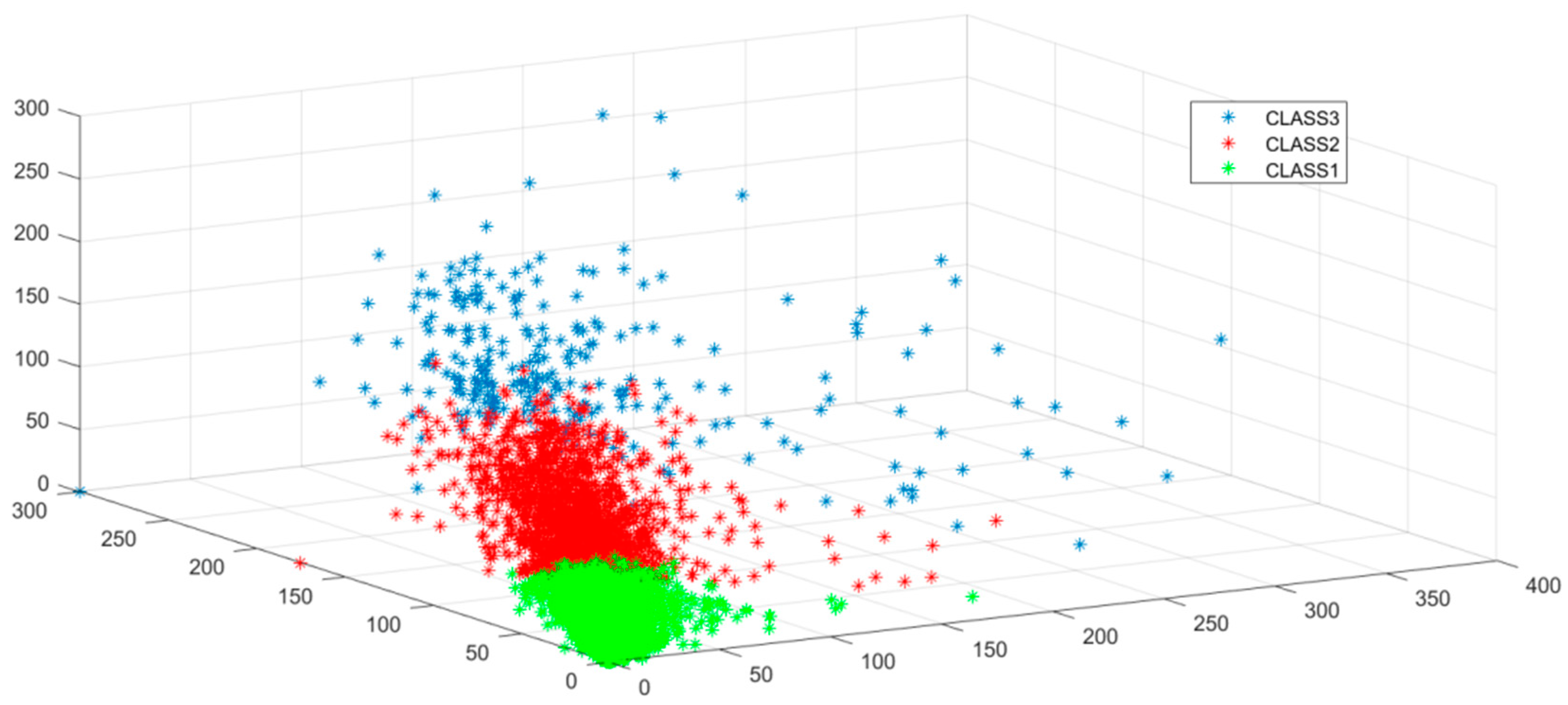
Figure 4.
Relationship between quarter sales and M.

Figure 5.
Relationship between mean sales and mean variance of grids, the x axis represents the average square deviation of each grid cell, and the y axis represents the average sales of retailers in each grid cell.
Figure 5.
Relationship between mean sales and mean variance of grids, the x axis represents the average square deviation of each grid cell, and the y axis represents the average sales of retailers in each grid cell.

Figure 6.
Spatial auto correction results of first class. Red grids represent the market demand of grid cells and nearby grids are high; Orange grids represent the market demand of them are medium; Transparent grids represent the market demand of them are small.
Figure 6.
Spatial auto correction results of first class. Red grids represent the market demand of grid cells and nearby grids are high; Orange grids represent the market demand of them are medium; Transparent grids represent the market demand of them are small.

Figure 7.
Dispersion degree evaluation of three areas.


Table 1.
Cluster centers of three types of shops.
| Class | Sales (α) | Sales (β) | Sales (δ) | Color |
|---|---|---|---|---|
| Class 1 | 148.65 | 114.36 | 148.83 | Green |
| Class 2 | 62.79 | 34.71 | 78.86 | Red |
| Class 3 | 17.61 | 12.58 | 20.60 | Black |
Table 2.
The fitting results of different Time Scale.
| Time Scale | Fitting Function | Goodness of Fit (R2) |
|---|---|---|
| Monthly | Y = −918.32x + 629,416 | 0.5072 |
| Quarterly | y = −49.592x2 − 1621.6x + 621,435 | 0.8984 |
Table 3.
Goodness of fit of two methods.
| Elementary Unit | Single Retailer | Grid |
|---|---|---|
| correlation function | y = −6.7318x + 560.48 | y = −0.0032x6 + 0.1162x5 − 1.5471x4 + 9.8235x3 − 35.369x2 + 55.349x + 391.65 |
| R2 | 0.287 | 0.733 |
Table 4.
Information of retail shops located in grids of 3 colors.
| Auto Correction Results | Shop Number | M* |
|---|---|---|
| Red | 75 | 5.9 |
| Orange | 141 | 8.6 |
| Transparent | 237 | 12.1 |
Table 5.
Sales situation of two groups.
| Group 1-Red | Group 2-Orange | ||||||||||
|---|---|---|---|---|---|---|---|---|---|---|---|
| ID | Products Sales | M* | Sum_Sales (Boxs) | ID | Products Sales | M* | Sum_Sales (Boxs) | ||||
| α | β | δ | α | β | δ | ||||||
| G1.1 | 95 | 125 | 134 | 4.66 | 361 | G2.1 | 73 | 30 | 96 | 8.47 | 199 |
| G1.2 | 203 | 130 | 135 | 4.90 | 468 | G2.2 | 62 | 47 | 59 | 9.12 | 168 |
| G1.3 | 125 | 79 | 101 | 5.25 | 305 | G2.3 | 50 | 26 | 43 | 12.44 | 119 |
| G1.4 | 164 | 81 | 75 | 6.81 | 320 | G2.4 | 80 | 32 | 44 | 9.68 | 156 |
| G1.5 | 108 | 71 | 82 | 7.36 | 261 | G2.5 | 59 | 24 | 107 | 8.50 | 190 |
| G1.6 | 119 | 110 | 138 | 2.58 | 367 | G2.6 | 71 | 27 | 72 | 9.53 | 170 |
| G1.7 | 87 | 105 | 98 | 6.62 | 290 | G2.7 | 73 | 53 | 84 | 7.14 | 210 |
| G1.8 | 159 | 91 | 118 | 3.28 | 368 | G2.8 | 81 | 29 | 62 | 8.85 | 172 |
| G1.9 | 108 | 101 | 154 | 3.54 | 363 | G2.9 | 68 | 50 | 124 | 6.55 | 242 |
| G1.10 | 144 | 58 | 109 | 5.70 | 311 | G2.10 | 70 | 66 | 60 | 7.35 | 196 |
| Average | 131 | 95 | 114 | 5.07 | 340 | 68 | 38 | 75 | 8.80 | 182 | |
Table 6.
Influence of different strategies.
| Red | Strategy1 | Orange | Strategy2 | ||||||||
|---|---|---|---|---|---|---|---|---|---|---|---|
| Theoretical Sales | _1 | Sale | Theoretical Sales | _2 | Sale | ||||||
| ID | α | β | Δ | ID | α | β | δ | ||||
| G1.1 | 95 | 125 | 134 | 4.66 | 361 | G2.1 | 73 | 60 | 96 | 8.47 | 199 |
| G1.2 | 203 | 130 | 135 | 4.90 | 468 | G2.2 | 70 | 39 | 59 | 8.96 | 198 |
| G1.3 | 128 | 100 | 128 | 5.07 | 356 | G2.3 | 65 | 36 | 18 | 10.62 | 184 |
| G1.4 | 128 | 100 | 128 | 5.07 | 356 | G2.4 | 68 | 37 | 51 | 9.24 | 191 |
| G1.5 | 128 | 100 | 128 | 5.07 | 356 | G2.5 | 90 | 54 | 107 | 8.50 | 190 |
| G1.6 | 119 | 110 | 138 | 2.58 | 367 | G2.6 | 69 | 38 | 64 | 9.17 | 192 |
| G1.7 | 128 | 100 | 128 | 5.07 | 356 | G2.7 | 73 | 83 | 84 | 7.14 | 210 |
| G1.8 | 159 | 91 | 118 | 3.28 | 368 | G2.8 | 72 | 39 | 61 | 8.83 | 202 |
| G1.9 | 108 | 101 | 154 | 3.54 | 363 | G2.9 | 103 | 80 | 124 | 6.55 | 242 |
| G1.10 | 128 | 100 | 128 | 5.07 | 356 | G2.10 | 70 | 96 | 60 | 7.35 | 196 |
| Average | 129 | 103 | 128 | 4.01 | 362 | 75 | 56 | 72 | 8 | 200 | |
© 2018 by the authors. Licensee MDPI, Basel, Switzerland. This article is an open access article distributed under the terms and conditions of the Creative Commons Attribution (CC BY) license (http://creativecommons.org/licenses/by/4.0/).
Share and Cite
MDPI and ACS Style
Wang, L.; Fan, H.; Gong, T. The Consumer Demand Estimating and Purchasing Strategies Optimizing of FMCG Retailers Based on Geographic Methods. Sustainability 2018, 10, 466. https://doi.org/10.3390/su10020466
AMA Style
Wang L, Fan H, Gong T. The Consumer Demand Estimating and Purchasing Strategies Optimizing of FMCG Retailers Based on Geographic Methods. Sustainability. 2018; 10(2):466. https://doi.org/10.3390/su10020466
Chicago/Turabian StyleWang, Luyao, Hong Fan, and Tianren Gong. 2018. "The Consumer Demand Estimating and Purchasing Strategies Optimizing of FMCG Retailers Based on Geographic Methods" Sustainability 10, no. 2: 466. https://doi.org/10.3390/su10020466
Note that from the first issue of 2016, this journal uses article numbers instead of page numbers. See further details here.