1. Introduction
Eutrophication, climate change, development, and overexploitation of both top predators and foundation species are driving the global loss and degradation of estuarine environments [
1,
2]. In the United States, only half of the historic salt marsh areas remain [
3]. Globally, about 85% of oysters have been lost, with most of the remaining reefs facing poor conditions [
4]. Many of these disappearing and degraded estuarine habitats occur on developed coastlines where high levels of human activity alter coastal food webs and waterways via shifts in water chemistry and hydrodynamics. In particular, recreational and commercial boat traffic is on the rise within estuaries worldwide and is significantly altering the hydrodynamics of these systems. Oyster reef survival has been shown to be limited by a narrow wave exposure threshold of 500 J/m [
5]. High-energy boat wakes can approach this threshold and contribute to mass oyster mortality along the edges of popular boating channels, as evidenced by dead reef margins that extend well above the high water line [
6]. Without the presence of oyster reefs, which provide natural shoreline protection, vegetation loss and erosion occur more readily [
7]. Both oysters and salt marshes play a vital role in coastal protection, nutrient filtration, and facilitation of biodiversity [
8]. These ecosystem services are hindered by constant disturbances from boating activity. Maintaining the natural, moderate energy regimes of coastal habitats in the face of heightened boat traffic is one of the greatest challenges in sustaining estuarine environments.
In estuarine environments, well-established vegetation and reef structures attenuate waves and boat wakes by diffusing momentum in the water column [
9]. While reefs serve as hardened biogenic breakwaters, plant stems and leaves reduce wave energy aboveground, while roots reinforce the soil below to thwart erosion [
10,
11]. Evidence suggests that after one year of growth at a wave tank facility, living shorelines comprising cordgrass (
Spartina alterniflora), oyster mats, and a sediment shoreline reduce wave energy by 67% percent (compared to 19% when newly deployed), which is largely due to a 130% increase in oyster density and a nearly ten-fold increase in plant density [
12]. Although vegetation and reefs provide some level of coastal defense, non-linear spatial and temporal irregularities inhibit their ability to provide consistent protection [
13]. Such variabilities could stem from hydrodynamic changes or density fluctuations due to age or stress. Narrow fringes are not sufficient for wave energy reduction, especially during extreme events [
13]. Disturbances to natural water regimes can also impact plant and oyster reef cover. For instance, patterns in oyster settlement and growth can be strongly influenced by water velocities, with larvae preferentially settling in low-flow refuges within high energy environments and growing faster in moderate to high velocity environments [
14]. Similarly, plant canopy height, root-to-shoot ratios, and density can respond to hydrodynamic conditions. Under sustained wave loading, plant roots loosen due to erosive forces stemming from steeply sloped marsh edges and thus contribute to further destabilization [
15]. In circumstances where emergent reefs and degraded vegetated edges are exposed to boat wakes that dramatically alter the hydrodynamic conditions experienced by plants and reefs, an additional energy break may be necessary to alleviate stresses incurred on fringes.
Several natural and engineered energy breaks have been introduced to shorelines in hopes of mitigating erosion. Hardened structures such as seawalls, bulkheads, riprap, or breakwaters are frequently placed in dynamic coastlines under the assumption that they will perform better and outlast other options [
16,
17]. While seawalls and bulkheads may be effective at reflecting wave energy, the structures induce seaward scour and halt natural upslope migration of vegetation in estuarine environments [
18]. This steepens the slope and ultimately leads to decreased species diversity [
19,
20]. In addition to these detrimental ecological effects, hardened shoreline options consisting of concrete or rock are often more expensive to build and maintain than living shorelines and are so heavy that they are inappropriate for shorelines characterized by soft sediment, where such materials would sink [
21]. As a result of these drawbacks to hardened shoreline options, practitioners have been deploying a variety of alternative structures including coconut fiber logs wrapped in coir matting and shell-based reefs as well as breakwalls built out of concrete granite mixed with shells [
22]. The cost and ability of these structures to withstand boat wakes without provoking significant sediment scour or loss of biodiversity varies, suggesting there remains an outstanding need to identify additional, cost-effective methods for mitigating shoreline erosion in many estuaries experiencing high boat traffic. This study experimentally tests the performance of one such breakwall design modeled after wooden groynes deployed widely in Europe to stabilize shorelines, minimize sediment scour, and mediate biodiversity. The test design entails the stacking of crepe myrtle (
Lagerstroemia indica) tree branches within wooden fence posts to create a relatively lightweight, durable, inexpensive, and semi-permeable wave and wake break along the shoreline edge. Similar porous brush bundle structures have been shown to reduce wave energy by 60% with a low-cost, simple installation [
23]. Porous structures are preferable to non-porous structures as they allow water to flow through them instead of acting as a hard, reflective wave barrier. This ultimately results in less scour. The optimal porosity of such porous structures is not yet known.
This interdisciplinary study combines the fields of ecology, geotechnical engineering, and coastal engineering to investigate a complex problem affecting estuarine habitats worldwide. The seemingly disparate topics of breakwalls, living shorelines, and boat wakes are presented together because they are heavily influenced by one another. The boat wakes are too energetic for oyster survival, which emphasizes the need to shelter them using breakwalls. However, the breakwall porosity must be carefully selected such that scour effects do not negatively alter oyster and plant habitat. Here, a statistical analysis of the boating climate along the Tolomato River is presented along with baseline data regarding site bathymetry and soil composition. The experimental design, based on National Oceanic and Atmospheric Administration (NOAA) guidelines for living shorelines, consists of a natural shoreline stabilization technique (oyster restoration structures) used in combination with a type of offshore sill/structure (breakwalls) [
24]. Additionally, a numerical model and a transmission analysis are used to assess the deflection and dissipation of the breakwalls under wave loading at various branch-generated breakwall porosities. Results regarding oyster and plant growth are not presented, as it is too early in the project to assess. Significant growth is anticipated by the end of summer 2018. The preliminary boat climate summary, background site data, and analysis of the porous breakwalls could assist others who are building living shorelines and designing estuarine management strategies. It is expected that this design will dissipate boat wakes such that sediment will accumulate, oyster reefs will develop, and the shoreline will progress seaward in areas protected behind the walls. Since little is known about the performance of living shorelines in moderate to highly dynamic environments, this study aims to provide valuable insight for coastal managers. In addition, boat traffic is a widespread issue that is not well characterized in many estuaries and thus this study addresses the lack of data on the magnitude and severity of this stressor.
2. Materials and Methods
The performance of these branch-based breakwalls was tested along the salt marsh-dominated shorelines lining the Intracoastal Waterway within the Guana Tolomato Matanzas National Estuarine Research Reserve (GTMNERR) in Ponte Vedra Beach, FL, USA. This site is ideal for this field study because of its popularity among boaters (Florida has the highest number of registered recreational boat vessels in the country) and because the salt marsh and fringing oyster reefs that dominate the shoreline edges are similar to those that characterize much of the southeastern US seaboard [
25]. Due to northeast Florida’s year-round temperate climate and proximity to several bodies of water, consistent boat traffic traverses through the study region. Based on a GIS (Geographic Information System) study using aerial photographs of the GTMNERR, close to 70 hectares of shoreline habitat along 64.8 km of channel margin have been eroded from 1970/1971 to 2002, with vessel-generated wakes suspected as the primary cause of this change [
26]. Depth, boat speed, and distance from the channel are all factors that influence wave height and erosion potential [
27]. For these reasons, the field sites were chosen to include a variety of channel widths displaying signs of recent, rapid marsh erosion.
2.1. Field Experiment
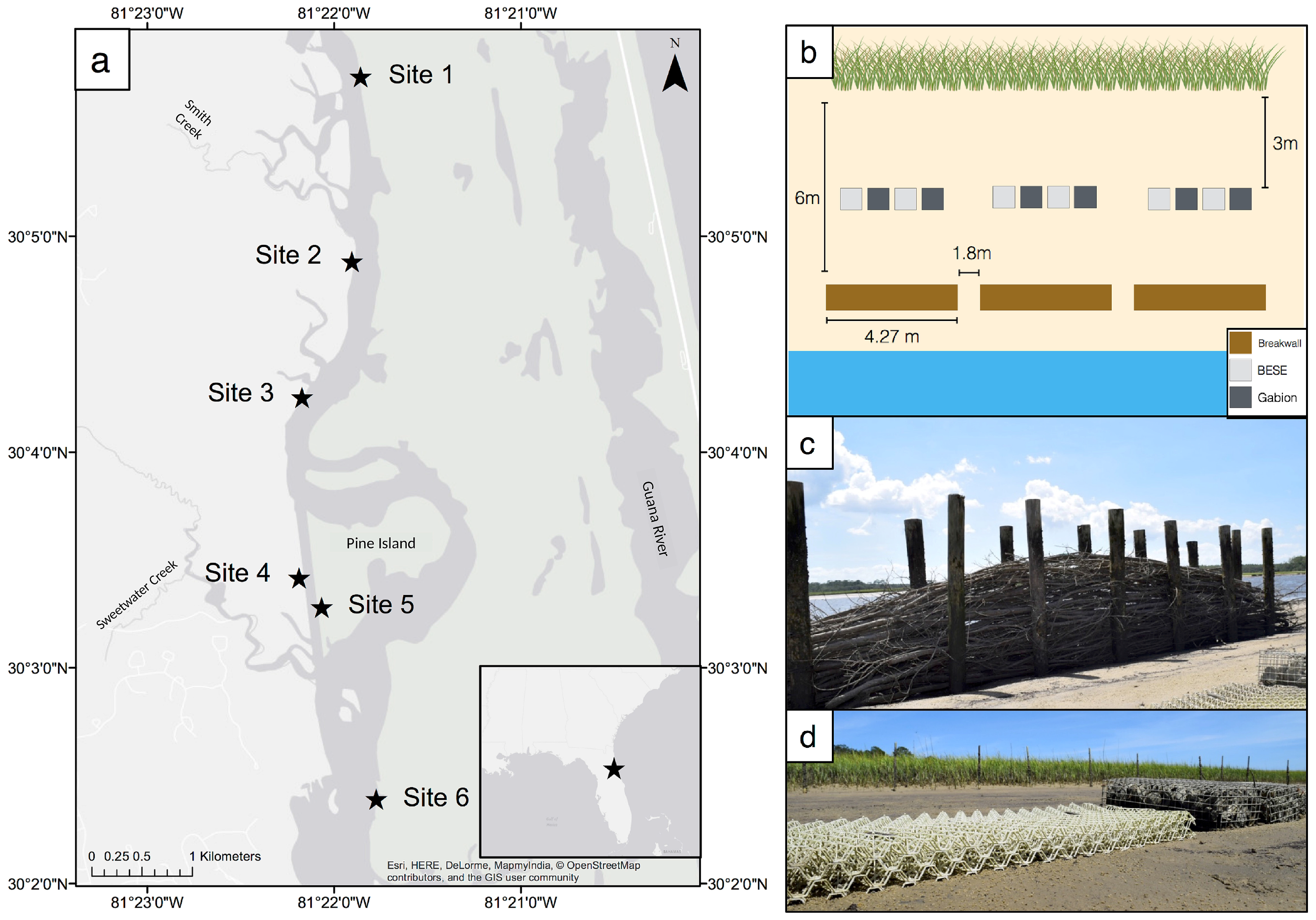
This research was conducted along the shoreline of the Tolomato River in the Atlantic Intracoastal Waterway, Ponte Vedra Beach, Florida, USA (
Figure 1a). These sites have an average tidal range of 1.6 m and are bordered on their landward edge by salt marsh habitat consisting mainly of cordgrass, along with some black mangroves (
Avicennia germinans) [
28]. Historically, eastern oyster (
Crassostrea virginica) reefs populated the edges of this estuary, but now they are predominately found in tidal creeks that experience lower levels of boating activity [
5]. However, the area still receives a steady oyster larval supply during the reproductive season, which lasts from March to October, with peaks in May–June [
29].
At each of the six study sites, three 14 m long segments of shoreline were delineated by using 15 Polyvinyl chloride (PVC) poles spaced 1 m apart. Each pole was inserted at the edge of the shoreline, defined as the seaward edge of the continuous peat mass. Two of these three segments of shoreline were designated as experimental treatments and one was left unaltered as a control; shoreline segments were spaced 30–40 m apart. Each treatment received a set of three wooden breakwalls located 6 m in front of the marked shoreline and spaced 1.8 m apart from one another. This orientation was utilized to enable the breakwalls to dissipate wave energy and facilitate sediment deposition in front of the seaward edge of the vegetation. One treatment received a set of low walls (approximately 30 cm high) and the other received a set of high walls (approximately 60 cm high) to evaluate their relative efficacy in stabilizing the shoreline. Behind each wall, four oyster restoration structures were placed 3 m in front of the shoreline edge (
Figure 1b).
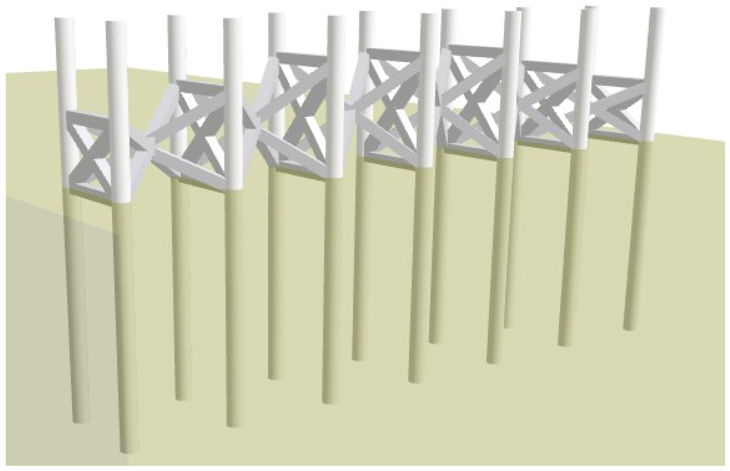
Each wall measured 4.27 m by 0.5 m (length by width) and was constructed between 10 February 2017 and 30 March 2017 using pressure-treated fence posts and crepe myrtle branches. Fence posts measured 9 cm in diameter and 2 m in length, and were cut on one end to form a sharp point to facilitate their insertion in the ground; each fence post was pounded into the ground to a depth of 75 cm. Crepe myrtle branches ranging from 1 to 8 cm in diameter and 1.5 to 4.27 m in length were harvested from live trees immediately before experiment deployment. Crepe myrtle trees are extensively used in local horticulture and are widely available. Landscapers routinely trim back their branches (which are adapted to resprouting upon trimming) in the winter/early spring, making it a free material to obtain for this experiment. Crepe myrtle branches are long, lightweight, and easy to transport, making them ideal staking material for the breakwalls. Each wall required 14 fence posts positioned in two rows of seven with crepe myrtle branches placed laterally between them (
Figure 1c). Branches were compressed and secured within the fence posts using plastic-coated wire arranged in a zig-zag pattern to prevent material from coming loose. Periodic maintenance is conducted, where the breakwalls are supplemented with branches if any have dislodged.
On 1 April 2017, four oyster restoration structures were installed behind each wall in a pattern alternating two types of structures: oyster gabions and Biodegradable Elements for Starting Ecosystems (BESE). Oyster gabions consist of wire cages measuring 51 cm by 20 cm by 15 cm (length by width by height) filled with oyster shell. BESE are potato starch structures consisting of multiple interlocking sheets that form a honeycomb-like pattern that can be stacked to a desired height. For this experiment, four BESE sheets were connected to form structures with dimensions of 90 cm by 45 cm by 6 cm (length by width by height) (
Figure 1d). The structures are expected to withstand this high-energy environment until reef formation, as they were secured in place with rebar behind the energy-absorbing breakwalls.
2.2. Topography and Geology
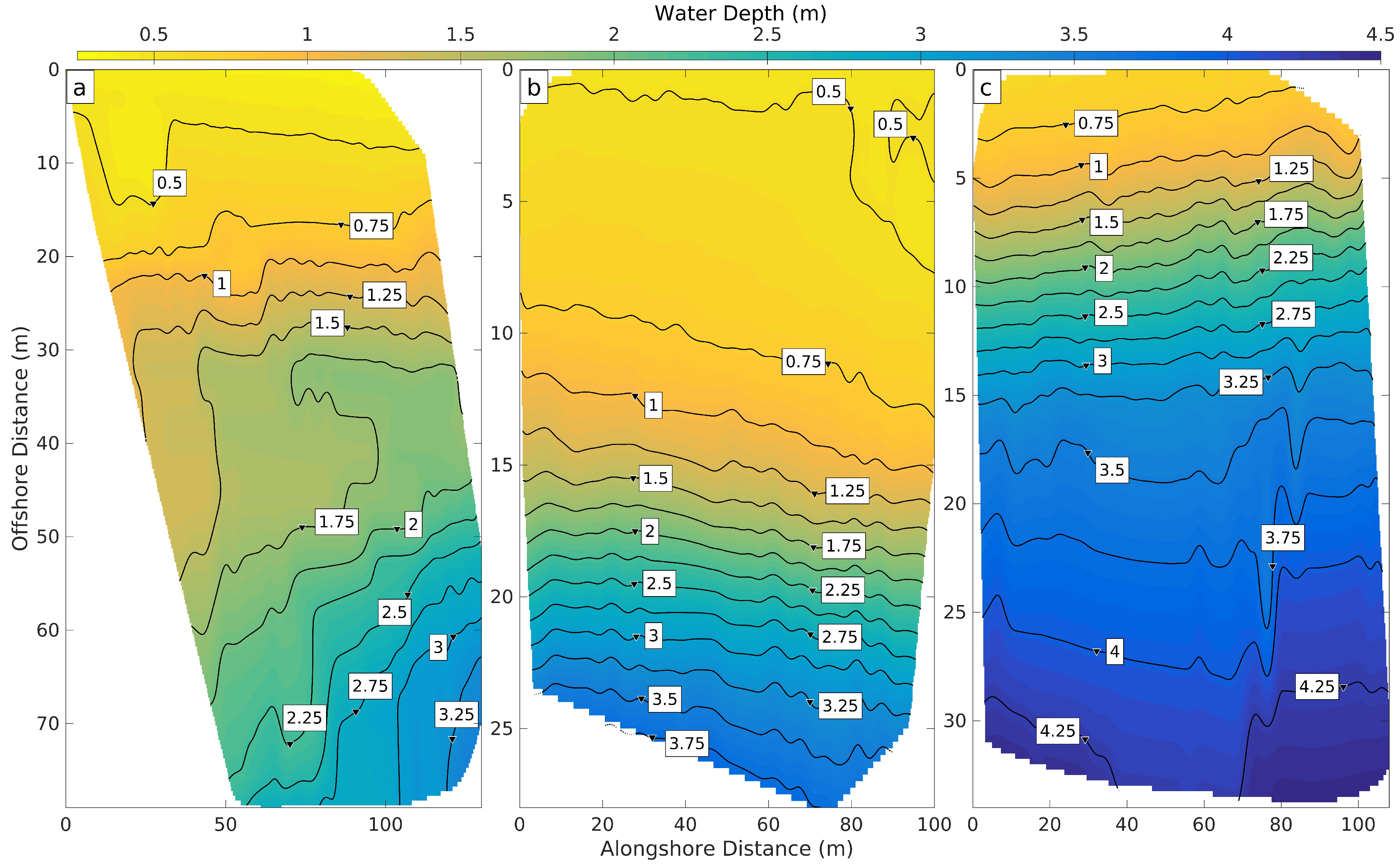
Bathymetric measurements were collected manually (using a tape measure) and with a Sontek PCADP (Pulse-Coherent Acoustic Doppler Profiler) at Sites 1, 3, and 4. These sites are located at varying channel widths (0.16, 0.32, and 0.1 km, respectively). Acoustic backscatter records from the PCADP were geolocated using a Trimble Geo 7x Global Positioning System. On 6 June 2017, the two instruments were attached to a boat that swept the interest areas. The PCADP recorded at two resolutions: 25-cm vertical bins in average water depths greater than ∼1.6 m according to the North American Vertical Datum of 1988 (NAVD 88) and 5-cm bins otherwise. After correcting for the instrument blanking distance and submerged depth, the maximum of the three-beam average of backscatter was identified as the location of the bed. Tidal records from the Florida Department of Environmental Protection (FDEP) at the Tolomato River were used to estimate the height of the tide above the mean mark at the time of each run [
28]. The tidal values were subtracted from the depth values for the corresponding time period utilizing NAVD 88.
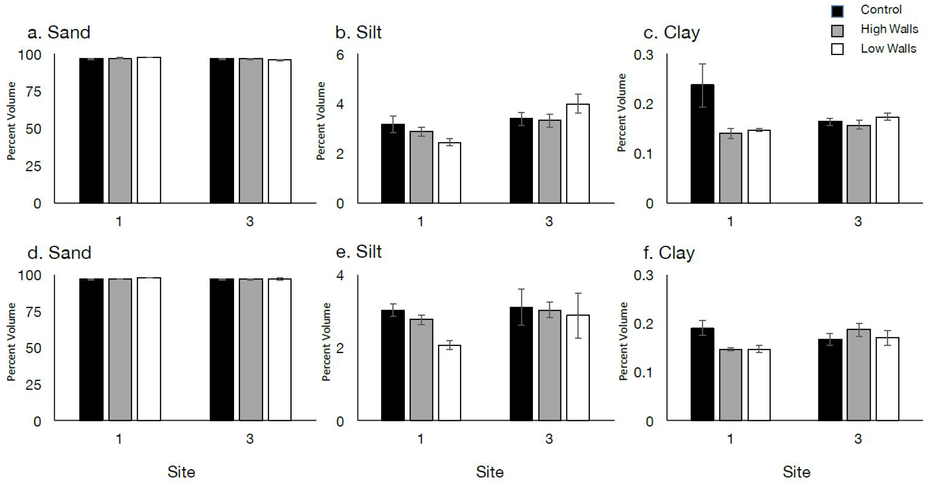
To assess the sediment grain size composition among sites and treatments within sites in order to set a benchmark for potential changes in the sediment due to the breakwalls over time, soil samples were taken at each treatment and control at both the lower intertidal zone and at the marsh edge at all sites. Soil samples were taken between 23 May 2017 and 24 May 2017 shortly after the installation of the breakwalls, thus establishing a benchmark from which to monitor future change. Samples consisted of three soil cores taken with a 2 cm diameter soil corer, which captured the top 10 cm of the sediment layer. For the lower intertidal zone, samples were collected 1 m shoreward of the low wall and high wall treatments, and at an equivalent distance from the shoreline for the controls. For the marsh edge, samples were collected at the PVC shoreline markers (see above for details).
In preparation for sediment grain size analysis, soil samples were oven-baked at 260
C for 24 h. Dried soil samples were analyzed using the Beckman Coulter Laser Diffraction Particle Size Analyzer (LS 13 320) under the Tornado Dry Powder System (DPS). LS 13 320 DPS measures the size distribution of particles suspended in dry powder form based on the principles of light scattering and produces a particle size distribution curve. At the drying temperature used, silt and clay drying in isolated interstices between 200
m sand grains will stay separated until shear is applied to liberate them from the sand bed. Dusting was observed when handling all dried powders. The elutriated particles in the air stream of the LS 13 320 DPS machine encountered an impact (during a 90 degree direction change) further liberating any particles clinging to the larger grains. Small agglomerates less than 0.4
m in size fall into the clay category (<2
m). The resulting curve is smooth and continuous from the starting value of 0.4
m to 40
m, indicating that silt and clay particles were indeed detected in using this technique (
Supplemental Figure S1). In combination with the United States Department of Agriculture (USDA) soil particle classifications, percentages of sand, silt, and clay were calculated for each of the samples. Mixed effect analyses of variance (ANOVAs) with site as a random factor and treatment as a fixed factor were used to compare variation in each grain size classification (percent of sand, silt, and clay) among treatments. Herein, data are presented for Sites 1 and 3 as representative measures of the sediment grain size observed across all study sites.
2.3. Wave Data Collection
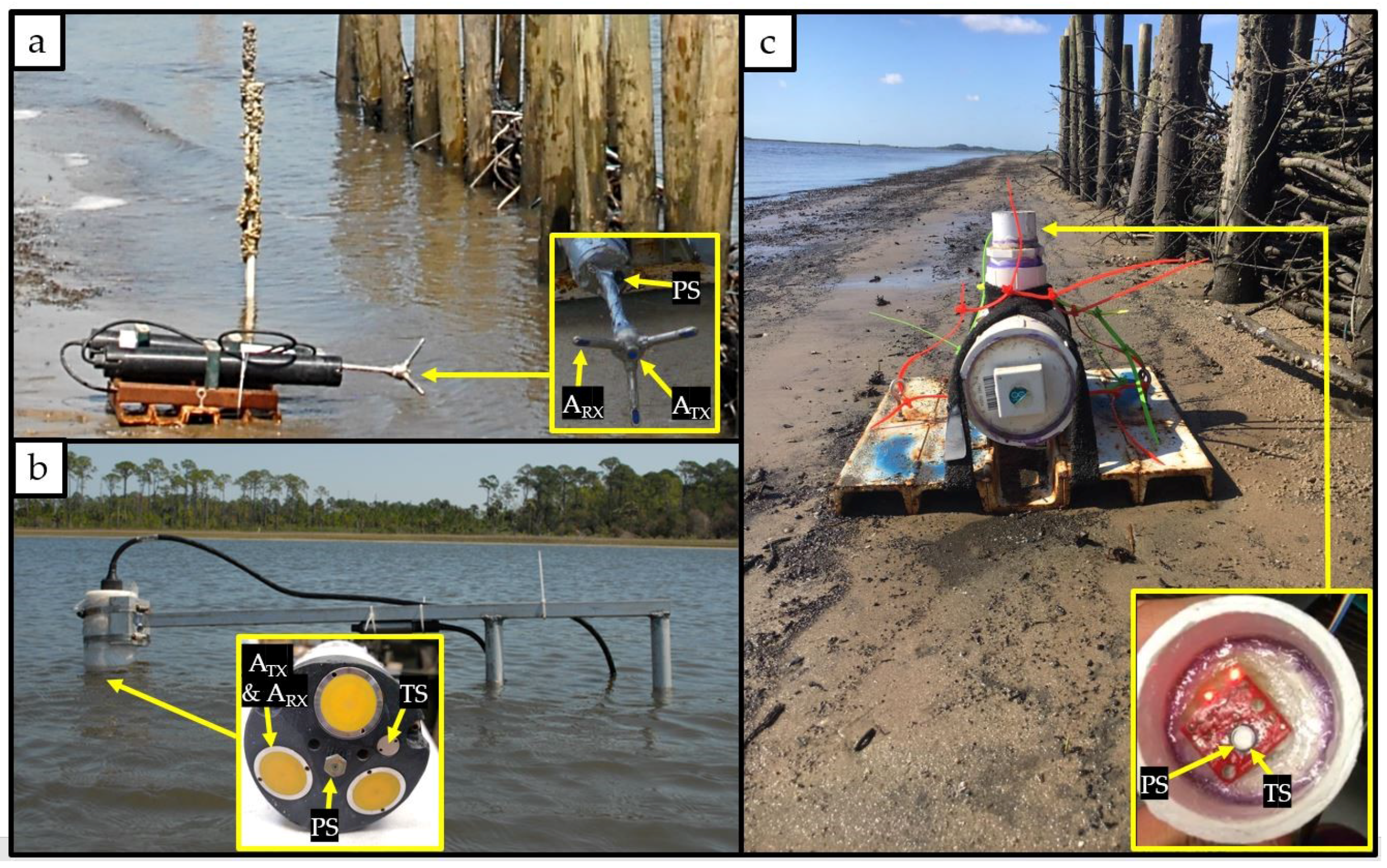
Three instruments were used to collect preliminary wave data at Site 4: a Nortek Vector ADV (Acoustic Doppler Velocimeter), a Sontek YSI PCADP, and a lab-created instrument named PEARL (Precision wavE Attribute Real-time Logger) (
Figure 2). The Vector was programmed to record backscatter and pressure at 16 Hz. PEARL and the PCADP recorded pressure at a sampling rate of 30 and 2 Hz, respectively. PEARL consists of an Arduino Uno R3 equipped with a 0.2 mbar resolution Adafruit MS5803-14BA Pressure Sensor, an Adafruit Data Logging Shield with an SD card, and a Tzumi 15,000 mAh battery. Every component except for the pressure sensor is housed inside a 10 cm diameter PVC pipe equipped with end fittings with a total length of 26 cm. One of the end caps is permanently fixed with PVC cement, where the other end is tightened and coated with RTV (Room-Temperature-Vulcanization) silicone before deployments to waterproof the housing as well as allow for easy removal. The pressure sensor has been potted inside a 4.5 cm diameter cap, filled with putty, and topped with layers of epoxy to ensure waterproofing in all areas except for the sensor face itself [
30]. When deployed, it was attached to an anchor with Velcro straps and zip ties. Prior to its deployment, it was calibrated in a pool at five different depths ranging from 0.165 m to 1.384 m, with an average percent error of 0.08%.
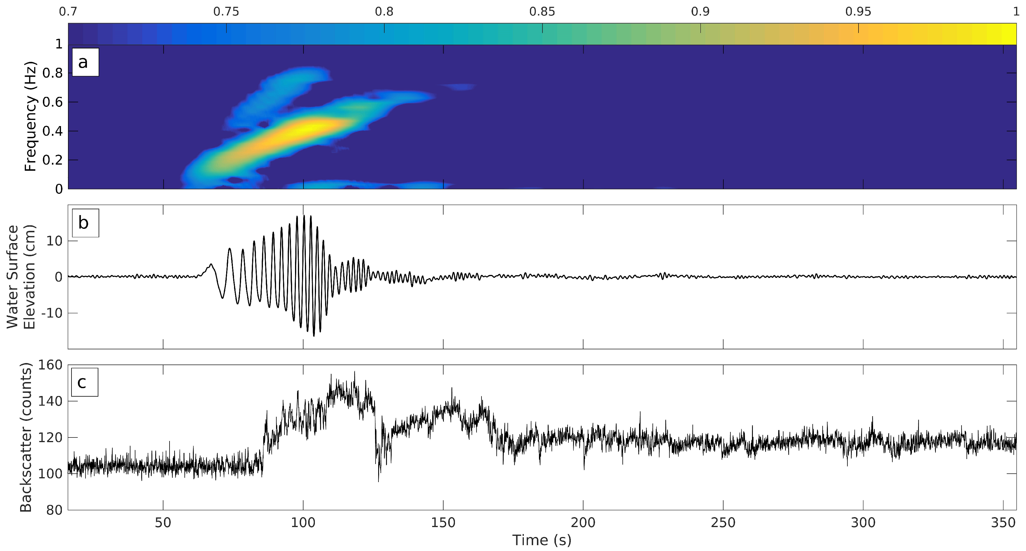
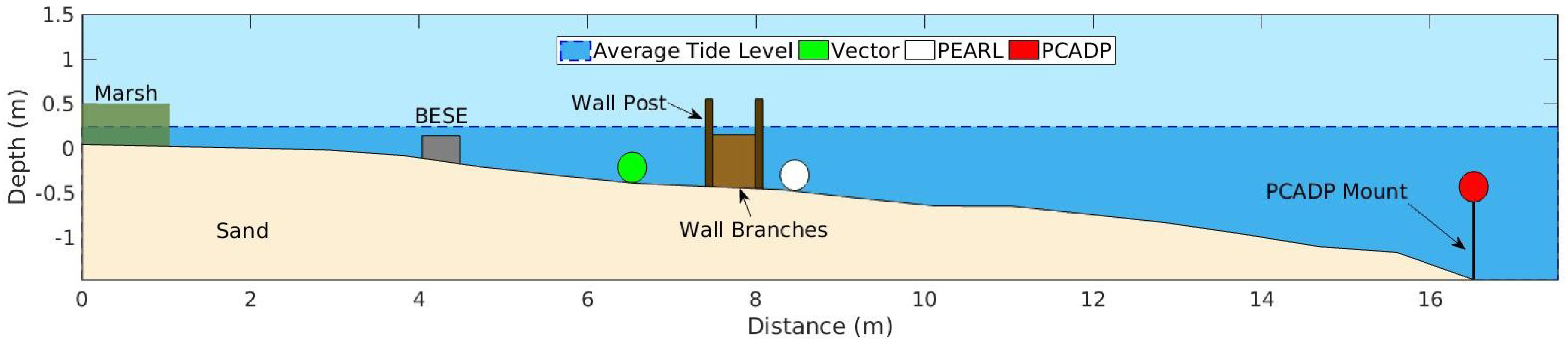
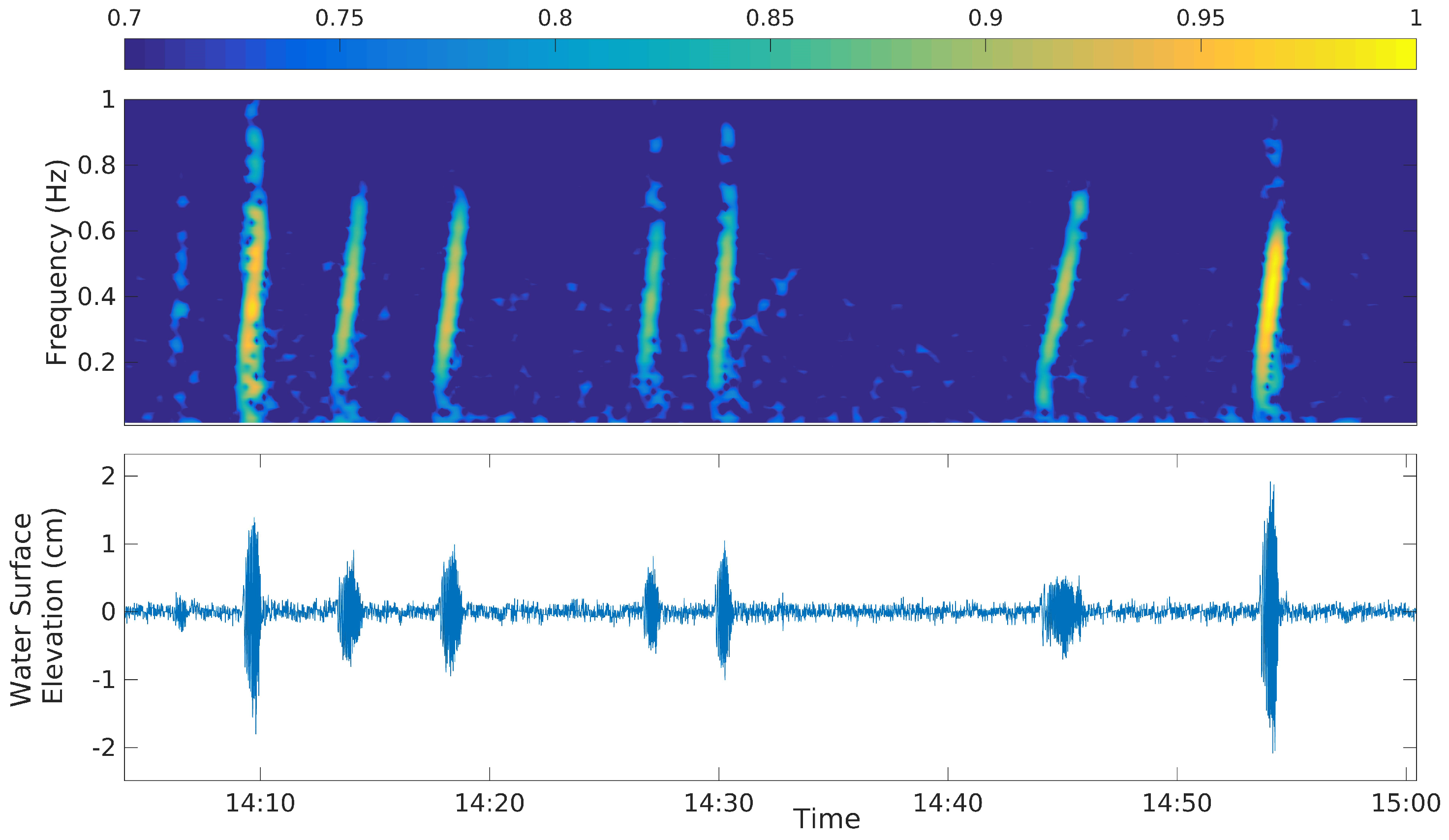
In March 2017, the Vector was placed 0.66 m behind the center of the southward wall set with the probe 10.16 cm above the ground. It recorded waves from 22 March 2017 to 25 March 2017 (
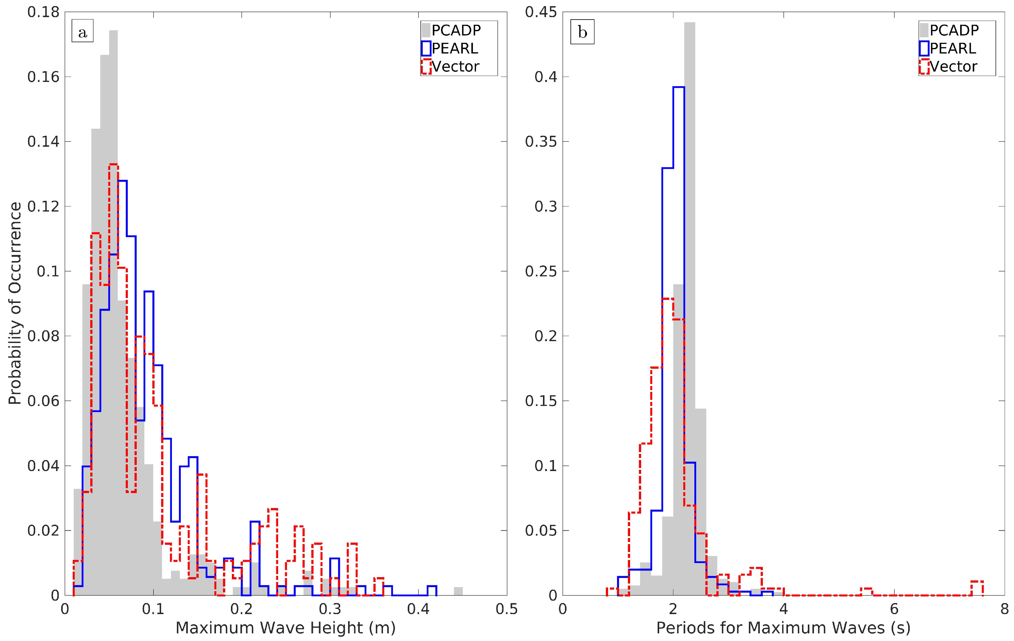
Figure 3). During this period of time, the breakwall height was 30 cm. For the next experiment in July, the wall height was increased to 60 cm. PEARL was placed 42 cm in front (seaward) of the center wall, while the PCADP was placed 8.53 m in front and 1.22 m north. The pressure sensors for PEARL and the PCADP were located 25.4 cm and 1.04 m above the ground, respectively. PEARL recorded from 13 July 2017 to 16 July 2017 and the PCADP recorded from 13 July 2017 to 17 July 2017.
2.4. Wave Analysis Methods
Pressure values for all instruments were adjusted to reflect relative pressure only. Atmospheric pressure values for the date ranges were taken from a nearby station on the Tolomato River operated by the FDEP [
28]. The instantaneous water depth
h was calculated using the hydrostatic pressure approximation
, where
p is pressure,
is salt water density (1025 (kg/m
), and
g is gravitational acceleration (9.81 m/s
). Tide (mean water level) and wave time series were separated using a simple Fourier filter which passed the entire signal through a direct and inverse Fourier transform sequence, with the inversion performed only for frequencies in the chosen band [
31,
32,
33]. Essentially, the same direct and inverse Fourier transform sequence was used to correct pressure time series of boat wakes for depth attenuation. For depth correction, a linear amplification factor was used:
where
h is the height of the instrument above the bed and
d is the average water level. The wave number
k and the radian frequency
satisfy the dispersion relationship
. Fourier transforms, spectrograms, and cross-spectrograms of pressure and velocity time series of boat wakes were computed using the MATLAB® implementation of the discrete, windowed Fourier transform. Wakes greater than 1 cm in height were identified by inspection, based on the spectrogram of pressure time series recorded by the instruments. Some wakes occurred very close in time and could not be separated from one another. In these cases, a multiplication factor was applied to account for all wakes. Individual waves within a wake were identified using a simple downward zero-crossing method. The wave with the largest total height (trough to peak) was used for statistical analysis.
2.5. Porosity
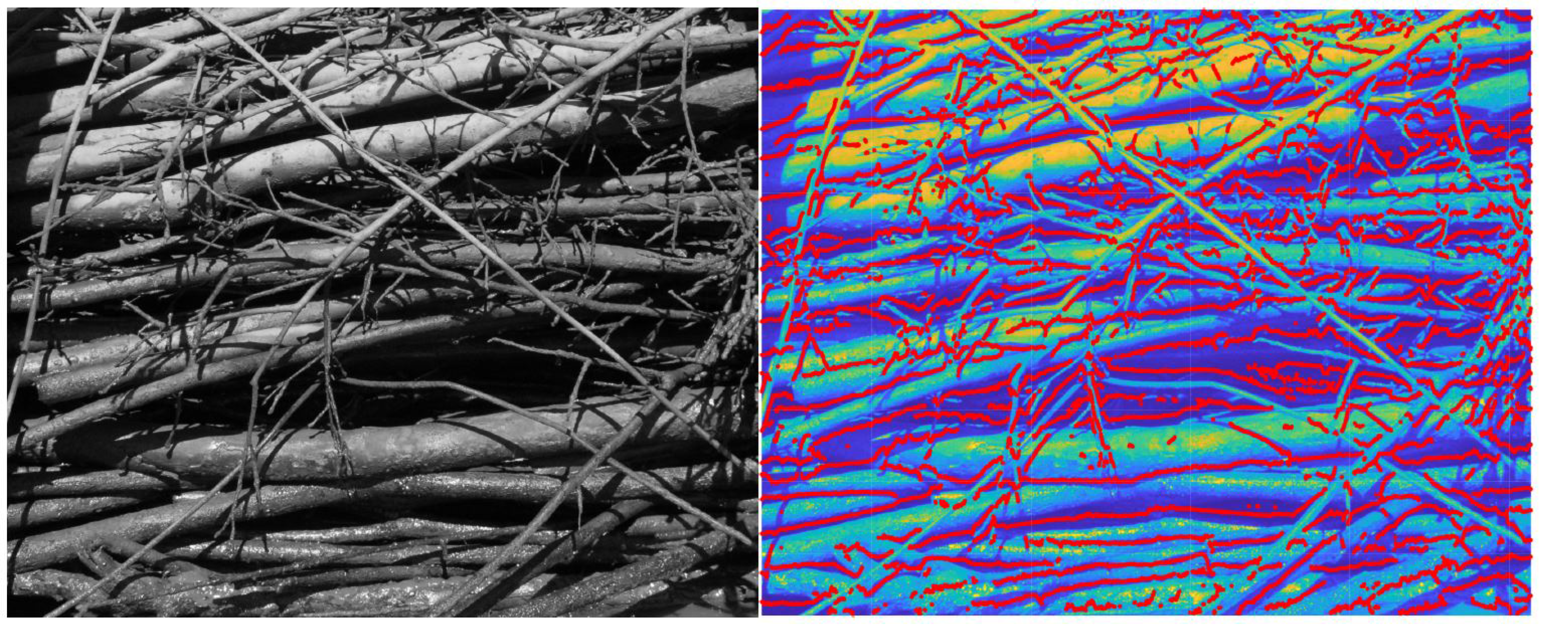
The porosity of the breakwall was estimated from an image analysis of eight photographs taken at the site. A simple algorithm that swept through all fixed columns in an image and detected luminosity edges was used to estimate the diameter of the branches. The breakwall was assumed to have the shape of a half cylinder of radius
R and the branches were assumed cylindrical. The porosity,
, was estimated as
where
A is the cross-sectional area of the breakwall half-cylinder and
is the diameter of branch
j, with
. However, allowance is made for the bias of the algorithm as well as the fact that each image only contains information about the visible branches in the visible part of the breakwall. To correct for these errors, three factors were introduced:
is a factor that compensated for specularity in the estimate of the branch diameter (the true diameter was
times the diameter
estimated using the edge detection algorithm);
represents the ratio of image height to the circumference of the half-cylinder, i.e., the height of an image is equal to
; and, finally, branches are seen inside the breakwall only to a depth of
times the mean branch diameter. It is difficult to establish the values of these three factors. These factors were given assumed values of
,
, and
= 2.
2.6. Numerical Modeling of Breakwalls
Models of the breakwall were developed to investigate their stability under wake loading. The model in
Figure 4 consisted of fourteen 2 m long piles with properties of southern pine (
E = 13.7 GPa,
= 100 MPa,
= 58.4 MPa,
= 0.65) embedded about 1.3 m below the mudline with two-dimensional beam elements attached to the piles [
34]. The beam elements have properties of crepe myrtle (
E = 10.8 GPa,
= 97.4 MPa,
= 64.1 MPa,
= 0.71) [
34]. The subsurface soil stratigraphy was determined through invasive Standard Penetration Tests (SPT) where physical samples were used to estimate soil stiffness and strength properties via SPT blow counts. Within the depths of interest, the stratigraphy can be described as 8–10 cm of soft loose silts and clays, followed by 1.8 m of loose to medium dense fine sand with silt, and finally underlain by 0.9 m of very loose sandy clay. Soil density, modulus, and strength estimates based on the blow counts were used to model the axial and lateral soil-pile interaction. The axial and lateral capacities were calculated according to methods for timber piles to be 1.22 kN of axial and 1.24 kN of lateral loading for a single pile [
35]. The soil was treated as saturated due to the wall location at high and low tides.
Wave loading on the breakwalls was simulated with the FB-Multipier finite element program [
36]. The program is capable of modeling soil-pile systems under dynamic conditions. The program uses the Wilson-Theta step-by-step integration procedure and iterates within each time step until equilibrium is achieved. The dynamic loading on the wall was calculated for the combined case of wave loading on a pile and fluid force acting within a porous structure. The force per unit length acting on the post lengths above the crepe myrtle branches was calculated using
where
is the dynamic wave pressure,
d is the post diameter,
is the drag coefficient (assumed to be 1.2),
is the density of saltwater,
is the wave velocity in the direction perpendicular to the wall,
is the inertia coefficient (assumed to be 0.8), and
is the component of local acceleration of the wave. The following equation
was used to determine the force per unit mass within the porous volume of the breakwall [
37]. The drag coefficient
was calculated according to
where the permeability coefficient,
for rubble stone mounds is assumed to be calculated according to
where
= 10 mm,
is the median diameter of the crepe myrtle branches, and
is the porosity of the breakwall [
38,
39]. In Equation (
5),
is in meters, where in Equation (
6),
is in millimeters. The inertia coefficient,
was determined according to
where
is an empirical coefficient taken to be 0.34 [
40].
The breakwall stability model analysis was performed using the average wake case measured by PEARL, which accounted for the local, near-wall wave heights. Each force (post and porous) was distributed over the length over which the dynamic force was acting.
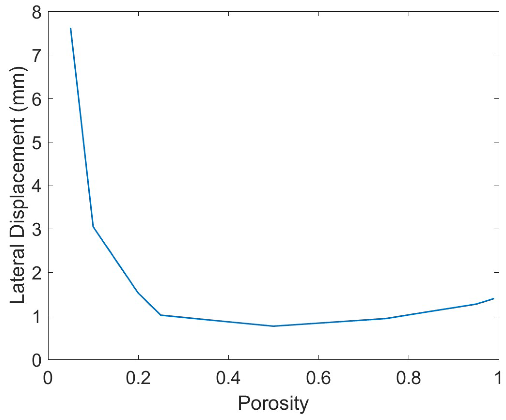
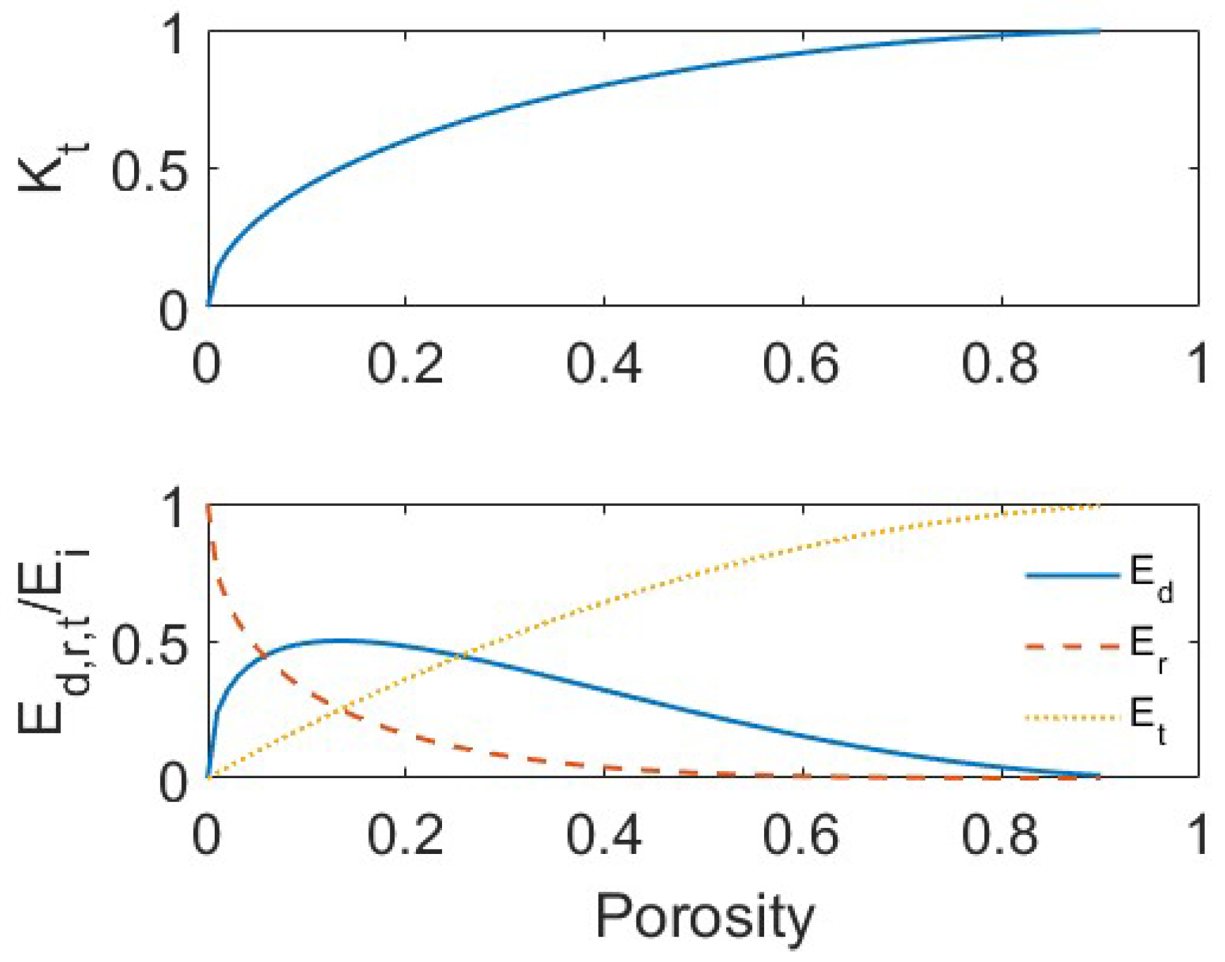
Figure 5 displays the thin elements of the breakwall model, the nodes at which the distributed forces are applied, and where the displacements in planar and vertical directions are solved through the iteration process. Of interest in assessing the stability of the wall against excessive bending was the demand to capacity ratio for forces in each direction. It was also necessary to limit lateral displacements, particularly in the case of a breakwall. Excessive lateral displacements can lead to gapping between the post and surrounding soil, resulting in more shear loads carried by the post and reduced axial capacity. With this analysis, wall porosities were selected, which correspond to the minimum lateral displacements.
2.7. Breakwall Transmission Estimation
The primary purpose of the breakwalls is to protect the vegetation and oyster restoration structures behind them by dissipating wake energy. While the simultaneous hydrodynamic measurements have not been made, the planned analysis of wake energy at different points can be discussed. To assess the effectiveness of a porous breakwall at dissipating wake energy, the wake transmission was determined, which was expressed as a transmission coefficient
where
is the transmitted wake height and
is the incident wake height (wake approaching breakwall). Wake reflection was accounted for with a wave reflection coefficient
where
is the reflected wake height. The following equation,
defines the relationship between
and
[
41]. The dissipated wake energy was calculated from
where the wake energy for each incident
, reflected
, and transmitted
components were calculated from Equation (
12).
With measured wake heights, the dissipated energy for a breakwall with a particular porosity was calculated using Equation (
13).
4. Conclusions
These findings conclude that the Intracoastal Waterway is a heavily trafficked boating area with an energetic wake climate. Boat wakes, especially from large or fast-moving vessels, suspend and transport nearshore sand particles into deeper water offshore ultimately leading to shoreline steepening [
46]. This is evidenced by backscatter values, which are consistently elevated during wake propagation. Waves as small as 10 cm can alter slopes in sandy/silty unvegetated areas [
10]. Major erosive events are believed to occur with wave heights between 30 and 35 cm [
47]. Numerous waves within these ranges were documented, which could be exacerbating erosion and vegetative retreat along the Intracoastal Waterway in Ponte Vedra Beach, FL, USA. Although wave data were only collected at one site, it is likely that the other five sites within the vicinity are experiencing comparable disturbances. This methodology could be applied to other parts of the Intracoastal Waterway facing similar threats from boat traffic.
Bathymetry plays a large role in the propagation and dissipation of waves [
42]. Wave fronts refract towards shallower areas as they shoal creating areas of divergence in addition to areas of convergence [
48]. Bathymetry is influenced by the type and size of sediment present. Environments dominated by large, coarse particles result in steeper coastal profiles [
42]. The sites are dominated by sand, which has a much larger particle size (0.05 to 2 mm) than silt (0.002 to 0.05 mm) and clay (<0.002 mm) [
49].
From the wall displacement and energy dissipation analyses, as seen in
Figure 12 and
Figure 13, a porosity that has both low displacement and high wave dissipation occurs at about 0.25. Although a low porosity breakwall of 0.25 may be ideal in balancing its stability in a hydrodynamic loading environment and dissipating wake energy, it is not suitable for a living shoreline. Low porosities result in the breakwalls acting more like hardened structures, which excel at reflecting wave energy, but result in environmentally damaging scour, shoreline steepening, and loss of plant and animal diversity [
18,
19,
20]. It is evident that an optimal porosity is challenging to determine due to the multifaceted nature of this topic. The analyses provided here are limited to the simplified wall parameters. Realistic variable branch diameter, roughness, and packing would influence the internal force distribution, wall deflected shape, energy transmission, scour, and sediment trapping effects. Diffracted waves could influence the wall loading and transmitted wave energy, depending on the incident wave lengths and distance between walls (aperture). The preliminary approach described here is focused on evaluating the magnitude of perceived leading order effects. This theoretical analysis is intended as a framework for future analysis based on complete and high-resolution datasets that will include simultaneous measurements in front and behind the breakwalls, as well as measured wall porosity (or void ratio) for various branch packings. The analysis of these datasets will include inspection for diffracted waves which will be included in subsequent modeling of the walls. Future studies will be carried out to address questions that have arisen regarding breakwall porosity values and their effectiveness in dissipating wave energy as well as mediating breakwall longevity in the face of damage due to shipworms and fouling organisms. Additionally, other wall characteristics will be investigated to help evaluate the current breakwalls and improve future designs. When the oyster reefs have successfully established, their impacts on the coastline will be assessed. At the end of this study, larger datasets from each specialization area (ecological, geotechnical, coastal) will make a valuable contribution to the existing literature, and it is anticipated that these porous energy-absorbing breakwalls will protect the salt marsh and oyster reefs from extreme hydraulic conditions and promote their growth.


