Article

How to Achieve Supply Chain Sustainability Efficiently? Taming the Triple Bottom Line Split Business Cycle †

by
Matthias Klumpp
1,2,3
1
Institute for Logistics and Service Management (ILD), FOM University of Applied Sciences, 45141 Essen, Germany
2
Robert Schuman Centre for Advanced Studies (RSCAS), European University Institute, 50014 Florence, Italy
3
Fraunhofer Institute for Material Flow and Logistics (IML), 44227 Dortmund, Germany
Sustainability 2018, 10(2), 397; https://doi.org/10.3390/su10020397
Submission received: 31 December 2017 / Revised: 27 January 2018 / Accepted: 29 January 2018 / Published: 3 February 2018
(This article belongs to the Special Issue Sustainable Supply Chains)

Abstract

:
For sustainable supply chains, specific concepts regarding how to efficiently improve sustainability are needed in a global comprehensive triple bottom line (TBL) approach, especially for forwarders as central actors in supply chain design. Such specific advice is provided by reporting empirical DEA Malmquist index findings from seven large European forwarders regarding a TBL sustainability analysis from 2006 to 2016. A major obstacle in improving sustainability consists in the newly discovered fact that with the business cycle, the three TBL areas of economic, ecologic and social objectives for logistics are undergoing different up- and down-ward trends, making it very hard to improve all three simultaneously. Additional factors are identified in the characteristics of size and government influence regarding the sustainability efficiency of forwarders. This has important impacts on supply chain design like e.g., with selection criteria.

1. Introduction

The objective of this paper is to search for explanatory factors towards sustainability efficiency with logistics service providers (LSP) as central supply chain actors in order to derive management design principles for sustainable supply chains in the future by changing such factors specifically. This is applied quantitatively and motivated by the following background.
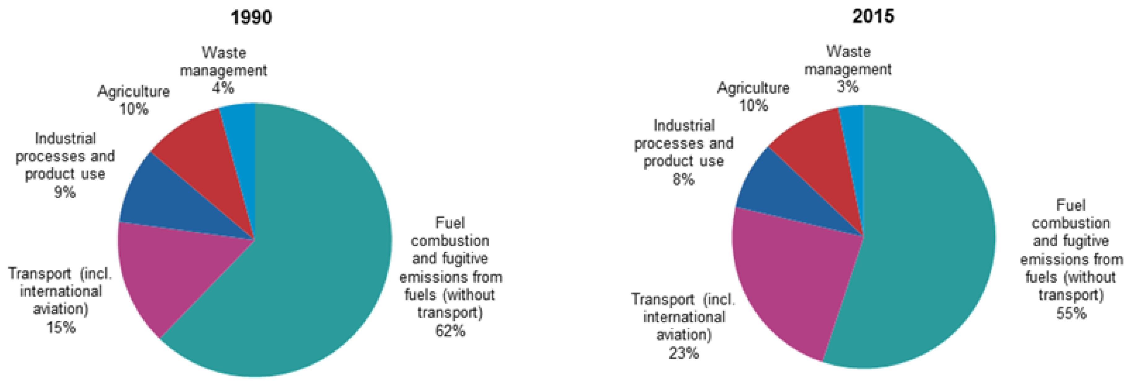
The transportation, logistics and supply chain management sector is very important for global sustainability as for example 2015 it accounted for 23% of greenhouse gas emissions within the European Union—up from 15% in 1990 [1]. This is connected to the question if logistics service providers (LSP) and forwarders as “designers” of supply chains are part of the solution or part of the problem. It is addressed for example within the publications by Vachon and Klaasen [2], Halldórsson and Kovács [3], McKinnon et al. [4], Mejías, Paz and Pardo [5], Golinska-Dawson and Kolinski [6], Sudarto, Takahashi and Morikawa [7] or Ma, Wang and Chen [8]. LSP plan and implement transport chains on behalf of industry and retail—thereby determining the sustainability setup and efficiency of manufacturers, suppliers, retailers and many other actors in global supply chains [9,10]. Additionally, technology advances provide further relevant results as suggested by Dijkema et al. [11] or Heiskala, Jokinen and Tinnilä [12]. Possible restrictions and problems include feared resource depletion and greenwashing [13,14,15,16]. For transportation, the global main transport modes road, rail, air and sea are challenged with sustainability concerns [17,18,19,20].
Sustainability conventions and political agreements are increasingly in place in order to prevent major negative consequences from the current and future human economic impact and general way of life of global warming and other adverse weather effects like storms, flooding and droughts; for example the following global contracts have been set in place historically in chronological order: the United Nations Framework Convention on Climate Change (1992), the Kyoto Protocol (1998), the Copenhagen Accord (2009), the Doha Amendment (2012), the Paris Agreement (2015) [21,22,23,24,25].
The modern state-of-the-art definition of sustainability has been provided by the Brundtland report in 1988 [26] (p. 16): “Humanity has the ability to make development sustainable to ensure that it meets the needs of the present without compromising the ability of future generations to meet their own needs.” As researchers state, this has been a step forward for defining and operationalizing sustainability, unifying economic, environmental and social objectives [27,28]. The specific word sustainability (“Nachhaltigkeit”) was introduced by the German von Carlowitz with the forest management objective not to cut more trees than can grow back in a “steady-state” timeline view [29].
Later on, this initial basis was developed further by important publications such as “Limits to Growth” [30]. From such global and societal sustainability objectives, corporate strategies and decisions are affected. Today, sustainability can be seen as a fundamental management philosophy embedded in the whole corporation, in all processes and decisions [31,32,33,34,35]. This has a specific impact on manufacturing, transportation as well as the logistics and supply chain sector. Growing interest in adopting environmental strategies along the entire supply chain can be recognized in research and business practice [35,36,37]. Several research approaches have been presented regarding sustainability, quantitative as well as qualitative ones [38,39]. A major result is the positive influence of collaboration towards improvements in economic as well as ecologic and social sustainability [40].
Supply Chain as well as general sustainability management approaches start with the claim to measure e.g., emission volumes in order to steer, manage and reduce them [41,42,43]. Regarding environmental indicators for transportation, logistics and supply chain management, the specific challenge becomes obvious that this sector has globally developed into the single largest contributor of greenhouse gas (GHG) emissions among all economic and society sectors—contributing for example 23% of total European EU-28 greenhouse gas emissions in 2015, see Figure 1 and [44].
Moreover, transportation is the only sector with a dynamic long-term increase in emissions, e.g., +16.5% for the USA between 1990 and 2015 (see Table 1). This does severely endanger the GHG emission reduction targets set specifically by the Paris Agreement. This picture is again consistent for different transport modes. In total, European (EU-28) emissions from transport (including aviation but excluding international shipping) in 2015 were 23% above 1990 levels—and this in contrast to a short-term recession decline between 2008 and 2013. Therein, international aviation experienced the largest increase in GHG emissions levels (+105%), followed by international shipping (+22% increase) and road transport, a +19% increase, [44].
Besides the environmental perspective, also a triple bottom line (TBL) approach including economic and social objectives and indicators is important in achieving sustainable supply chains. Therefore, also LSP are required to steer their management and design concepts—and research should contribute to this by suggesting and implementing matching measurement and management concepts in order to improve also in the social and economic sustainability domains.
However, what could an individual LSP contribute to those aggregate economic and society objectives? The important role of single LSP companies is given by a required efficiency increase as a political overall de-growth or limitation of growth strategy is not aimed for [45,46]. In order to allow for a moderate and balanced economic and social development and growth, LSP would have to improve their efficiency significantly within all three TBL dimensions e.g., by aiming to reduce the GHG emission volume per tonkilometer of transport service—comparable to the quality-efficiency nexus proposed by Du [47]. This entails business risks but as the overall transport volume and therefore the absolute total GHG emission is out of their individual decision environment, this is the only way forward for sustainability improvements from the individual LSP perspective [48,49]. This is also exemplified by specific triple bottom line objectives within corporate strategies and reports like e.g., Deutsche Bahn [50] (p. 58) or Deutsche Post DHL [51] (p. 76). Many research avenues and projects therefore address such questions, mainly aiming to reduce and optimize the logistics “footprint” [52,53,54,55]. As was experienced involuntarily during the 2008 economic crisis, the total amount of GHG emissions can easily be reduced by lowering the overall transport volume. This is a political question at the core—and significantly complicated in a dynamic perspective by the Jevons paradox [56,57]. However, furthering a relative measurement approach, this research work will try to establish relative measures of sustainability performance for LSP, e.g., by comparing GHG output volumes to asset and other corporate input indicators. Therefore, also in another size-related dimension, the question of corporate size and absolute transport volume does not come into account with this longitudinal efficiency analysis. Derived from this, the importance of sustainability efforts in the transportation and supply chain sector is reflected by the fact that major LSP provide sustainability data and evaluations e.g., in financial report documents, supporting organizational change and driving firm value [58,59,60]. Although a variety of communication and research regarding sustainability in logistics has been published, empirical evidence for sustainability improvements is largely missing. Quantitative research is of interest towards the productivity and efficiency of LSP regarding the established triple bottom line (TBL) approach, including economic, environmental and social performance areas, especially for a dynamic time-series perspective. Therefore, for example the operations research technique data envelopment analysis (DEA) Malmquist index calculation can be used in order to provide a time-series calculation of sustainability efficiency for multiple objectives regarding the TBL approach—this is applied herein and explained further below. The final objective of this endeavour is to establish explanatory factors towards such sustainability efficiency with LSP in order to derive management design principles for sustainable supply chains in the future by changing such factors specifically.
The specific contribution of this paper is a quantitative long-term analysis with DEA Malmquist index efficiency analysis for European LSP 2006 to 2016 in order to identify factors for efficiently improving supply chain sustainability by increasing the efficiency in TBL indicators with LSP.
The remainder of this paper is structured as follows: Section 2 outlines method and data for the applied quantitative DEA Malmquist analysis. Section 3 provides the results for seven European LSP regarding sustainability. Section 4 describes a discussion regarding these results. Section 5 ads a dynamic simulation model regarding the discussed problems for supply chain sustainability—and finally, Section 6 concludes with interesting further research questions.

2. Method and Data

2.1. Efficiency Measurement

Efficiency measurement can be divided methodology-wise in parametric and non-parametric techniques for application towards specific research questions. Whereas parametric models do have advantages regarding statistical quality measures and assurance levels, they do require a detailed understanding of the production process including a specific notion for a production function form to be applied in the data analysis [61,62,63]. Non-parametric approaches on the other hand do not require in-depth knowledge and prior data regarding the specific production processes; they simply use the available real-life input and output data for an efficiency measure. This is the suitable approach especially for the sustainability TBL questions offered here as no sensible production theory and function information can be surmised regarding a multitude of TBL sustainability output indicators.
Therefore, we proceed with the application of non-parametric concepts. One of the most used techniques in this branch, the data envelopment analysis (DEA) was developed from works of Koopmans in 1951 regarding the activity analysis concept [64], Debreu [65] and Farrell in terms of the radial efficiency measure [66] as well as works of Diewert [67]. This led to the specific DEA method suggestion by Charnes, Cooper and Rhodes in 1978 [68]. Advantages of the increasing use in management research are the facts that no a priori existing knowledge of a production function is required, only real-life data is used (no hypothetical production function or efficiency values); and a multitude of inputs can be combined with a multitude of outputs, which is very typical for LSP as complex and high-level service providers as well as other service industries like health care or higher education [69,70,71,72,73].
DEA studies Decision Making Units (DMUs), which can be seen as the entities responsible for input, throughput and output decision making. DMUs like LSP can be evaluated and compared, showing a specific level of decision making success in terms of overall efficiency. DEA uses a non-parametric mathematical programming approach for this evaluation of DMUs’ efficiency relative to each other. Furthermore, it is assumed that there are several DMUs and it is supposed that inputs and outputs comply with the following requirements: (i) For each input and output, there are numerical, positive data to be chosen for all DMUs; (ii) Selected values (inputs, outputs and the chosen DMUs) should depict the interest of decision-makers towards the relative efficiency evaluations; (iii) DMUs are homogenous in terms of identical inputs and outputs; (iv) Input and output indicator units and scales are congruent. Furthermore, two different basic models can be distinguished. The CCR model (named Charnes, Cooper and Rhodes [68]) with constant returns to scale and the BCC model with variable returns to scale (Banker, Charnes and Cooper [74]). One basic characteristic of the constant returns to scale CCR model is the multi-output and multi-input reduction to a single (weighted) input and output combination for each DMU. For a certain DMU, measuring its efficiency and comparison with other DMUs in the system is enabled.
Further on, based on early works of Malmquist [75], Caves, Christensen and Diewert 1982 [76] proposed a calculation of a productivity index in order to shed light on efficiency changes over time. This new longitudinal perspective is especially promising for the DEA method as most efficiency measurement approaches are directed towards the question of efficiency improvement. In order to provide usable information for this objective, the index is therefore distinguishing between a technological progress for the whole set of DMUs—individually adapted for each institution—on the one side and the technological efficiency on the other side [77]. A series of applications do exist for this specific longitudinal efficiency analysis, as shown for example by Thanassoulis, Shiraz and Maniadakis [78] for water and gas companies from different countries, Emrouznejad and Yang [79] for CO2 emissions of Chinese manufacturing, Sueyoshi and Goto [80] for the environmental evaluation of petroleum companies, or Chang, Kuo and Chen [81] for a pollution evaluation in China.
Alternative longitudinal analysis techniques based on DEA are for example the DEA window analysis [82,83] as well as the dynamic network DEA (see e.g., Guo et al. [84] or Khushalani and Ozcan [85]): For the DEA window analysis e.g., Vlontzos and Pardalos [86] outline a longitudinal efficiency analysis regarding the GHG emissions from EU agricultural industries. Similarly, Halkos and Tzeremes [87] have analysed the hypothesis of an environmental Kuznets curve with this technique. Further applications include e.g., the energy sector [88] or hospital services [89,90]. Though powerful, DEA window analysis does not provide the advantage of differentiating between a general technological advance (production frontier shift) and the individual DMU efficiency development. Therefore, in this paper the advantageous Malmquist index is applied.

2.2. Sustainability Data

Determining the analysis area, the European region within a global logistics market is selected for three reasons. First, within the European business environment, a large number of companies are active within a comparable corporate reporting and business environment, enhancing comparative strength of the analysis. Furthermore, though the industry is built up mainly out of very small and medium-sized companies, in Europe there are at least some large integrators. And finally, those larger companies are required to publish detailed business and corporate data in their financial reporting according to international standards as well as CSR and environmental data. For detailed evaluation and analysis, seven European-based but internationally active LSP are analysed according to different market share and leadership sources. DB Schenker, DHL, DSV, Kühne + Nagel, La Poste, Panalpina and SNCF (see Table 2 for corporate size and data).
The complexity of CSR and sustainability efficiency evaluations is highlighted for example by diverse statements in the companies’ business reports, among them the following interesting strategy analysis from La Poste, an international logistics groups historically stemming from the French postal services (see Figure 2).
Regarding a sensible input indicator for a sustainability efficiency calculation, the analysis based on corporate reports of globally active LSP led to two feasible indicators: (i) Asset volume—The total asset value as reported in the financial reporting of the selected LSP is used; (ii) Revenue volume—The total revenue volume is included as indicator for corporate and activity size for input evaluation.
Sustainability has been operationalized among other research works by the TBL concept according to Elkington [92] as well as further extensions and adaptions [93,94,95]. For output indicators along the TBL concept the following items are selected: A largely neglected field is the social dimension (“people”; see [96,97]). Herein mainly working rights, safety as well as equal and fair pay questions are addressed [98,99]. However, in most sustainability discussions the social dimension is rooted in the corporate role as employer, providing income, participation and status to people around the world. But again, this is not the whole story. Moreover, diversity and gender questions are also increasingly addressed in this domain [100,101]. Regarding social analysis, the following two output types are used as indicators and included in the subsequent analysis: (iii) Employment—As the core social role for companies is to provide work and income, the full-time equivalent (FTE) figure from the corporate LSP reports (usually figure at year end/31.12.) is taken as output type for social sustainability. Headcount figures allow for serious influence potential as full positions could be sliced into part-time positions and therefore increase headcount without raising total personnel cost. Though it may be argued that the headcount is more adequate for the social role (providing participation, opportunities, training and education), in this case the influence risk potential is valued more important and therefore FTE numbers are included; (iv) Gender equality and woman participation in management. This share is valued as an important and comparable indicator for the social sustainability and success of LSP in this evaluation. In some cases where the reported numbers are not available for all subsequent years of analysis, the older numbers were assumed to be at least at the level of the latest reported figure. This assures that no company has disadvantages in this point given the fact that these shares are continuously rising in tendency.
The environmental perspective of “planet” within the triple bottom line approach is in the vast majority of research papers concerning itself with the climate change and carbon emission problem area as e.g., outlined by Wang and He [102] for regional transportation sectors in China or Voytenko et al. [103] for the development of sustainably cities in Europe. Regarding environmental analysis for the subsequent efficiency development analysis, the following output type is used as indicator: (v) Carbon emission volume—The measured and reported scope 2 GHG emissions in million tonnes of carbon dioxide equivalents are used as a valid output indicator for the environmental sustainability.
The established corporate perspective of economic viability and success (“profit” perspective) is widely acknowledged and the aim of many research and management science optimization quests [104,105]. Regarding this, the following two output types are used as indicators: (vi) EBIT—The yearly corporate profit as measured by the earnings before interest and tax (EBIT) standardized figure in corporate reporting. All currency quantities are converted to Euro values according to OECD historical exchange rate data [106]; (vii) Dividend Volume—As a further yearly economic performance indicator the total dividend volume paid to the shareholders is used.
Table 3 below is outlining major characteristics and correlations regarding these indicators to be used in the following calculations. Negative EBIT values have been replaced by a “0.01” as such negative values as well as zero values cannot be computed with the applied DEA technique (italics) due to quotient calculation; the output item GHG emissions is technically computed as an input type as the optimization direction is towards reducing the volume of GHG emissions like other input types. Data and calculation are a significant extension of an earlier study in 2017 with only five LSP and the timeframe of 2006 to 2015 only [107]. This was extended significantly by incorporating seven LSP and the longer timeframe of 2006 to 2016 (eleven years).

3. Results

The calculation results have been obtained for the presented input and output data in the timeframe 2006 to 2016 while applying an output-oriented DEA Malmquist index model with the software BANXIA Frontier Analyst for the named LSP. Three different variations in the calculation runs were tested as follows. First, it was tested if the inclusion of the input type “assets” does have an impact on results. It was concluded that the impacts of including this specific indicator were negligible and therefore due to a larger information basis the input type was included in further calculations. Second, the assumption regarding returns to scale modes was tested. This differs in the assumption of “constant returns to scale (CRS)” or “variable returns to scale (VRS)” due to production theory and DEA technique method background [66,183]. Both models were calculated and are reported in an aggregate version in the following Table 4. As VRS scale assumptions show higher levels of efficiency, this is the correct assumption for this analysis setting.
Third, minimum weightings of 10% were tested for the feasible input types (assets, revenue) and output types (GHG emissions, employment, women participation). The output types EBIT and dividend volume are mathematically not feasible for this instrument as zero values exist and pre-ordered weighting for such values would result in unrealistically low efficiency values. The introduction of minimum weightings is a standard choice with the objective to achieve satisfactory discrimination levels [184]. This also connects to the idea of the triple bottom line as in the pure application of DEA without minimum weighting restrictions it would be allowed for single LSP to individually factor out specific areas of the triple bottom line. This would obviously counteract the basic idea of the triple bottom line approach. Results are also reported in Table 4, coming up with four different calculation cases. As the introduction of weightings obviously secures differentiation, data from run D was used further for discussion. This is representing a good compromise as with five indicators and 10% minimum weighting, an overall sum of 50% out of 100% weighting are “fixed” for the five input and output types—whereas the other 50% can be freely attributed by the DEA technique’s internal method algorithm. Therefore, this analysis approach guarantees a required triple bottom line representation as well as a freedom for each DMU (LSP) to develop a specific profile regarding the three triple bottom line areas (see Table 4).
Regarding the overall statistical characteristics outlined in Table 4 like arithmetic mean or median values for the resulting efficiency values, we recognize familiar effects. First, CRS model calculations both (A and C) show lower efficiency levels than the VRS model calculations (B and D). This is due to more restrictive convexity assumptions in the basic production frontier model. But the VRS case is more realistic as differences occur [185,186]—and this connects to many business experience items with LSP being able to use economies of scale not proportionally but only to a certain extend depending on their actual size and business model (economies of scope or density). Therefore, for further analysis calculation runs B and D seem more appropriate. Second, introducing the 10% weighting for the applicable five input and output types (D) provides lower efficiency levels and therefore improved discrimination, highlighted by higher standard deviation (5.74% over 2.12%) and minimum efficiency values (62.7% versus 82.4%). Therefore, in order to provide applicable management advice, the more discriminating model run D is used for further analysis. Below, main results regarding efficiency developments 2006–2016 for model run D are described as basis for the subsequent discussion of results (Table 5 and Figure 3).
From the results depicted in Table 5 it is recognizable that the four LSP DHL, Kuehne + Nagel, La Poste and Panalpina are featuring efficient operations with an efficiency score throughout the whole analysis timeframe 2006–2016 of 100%. Whereas DB (Schenker), DSV and SNCF are experiencing lower efficiency scores, at least in specific years. Among the three, it is interesting to see that DSV incurs “increasing” economies of scale regarding overall production volume (being, so to say, “too small to reach higher efficiency levels”)—whereas DB and SNCF as large former state railway conglomerates are indicated to have too large a production volume (meaning “decreasing” returns to scale). More interesting than the yearly absolute efficiency scores per LSP are the longitudinal efficiency developments throughout 2006 to 2016, additionally shown in 
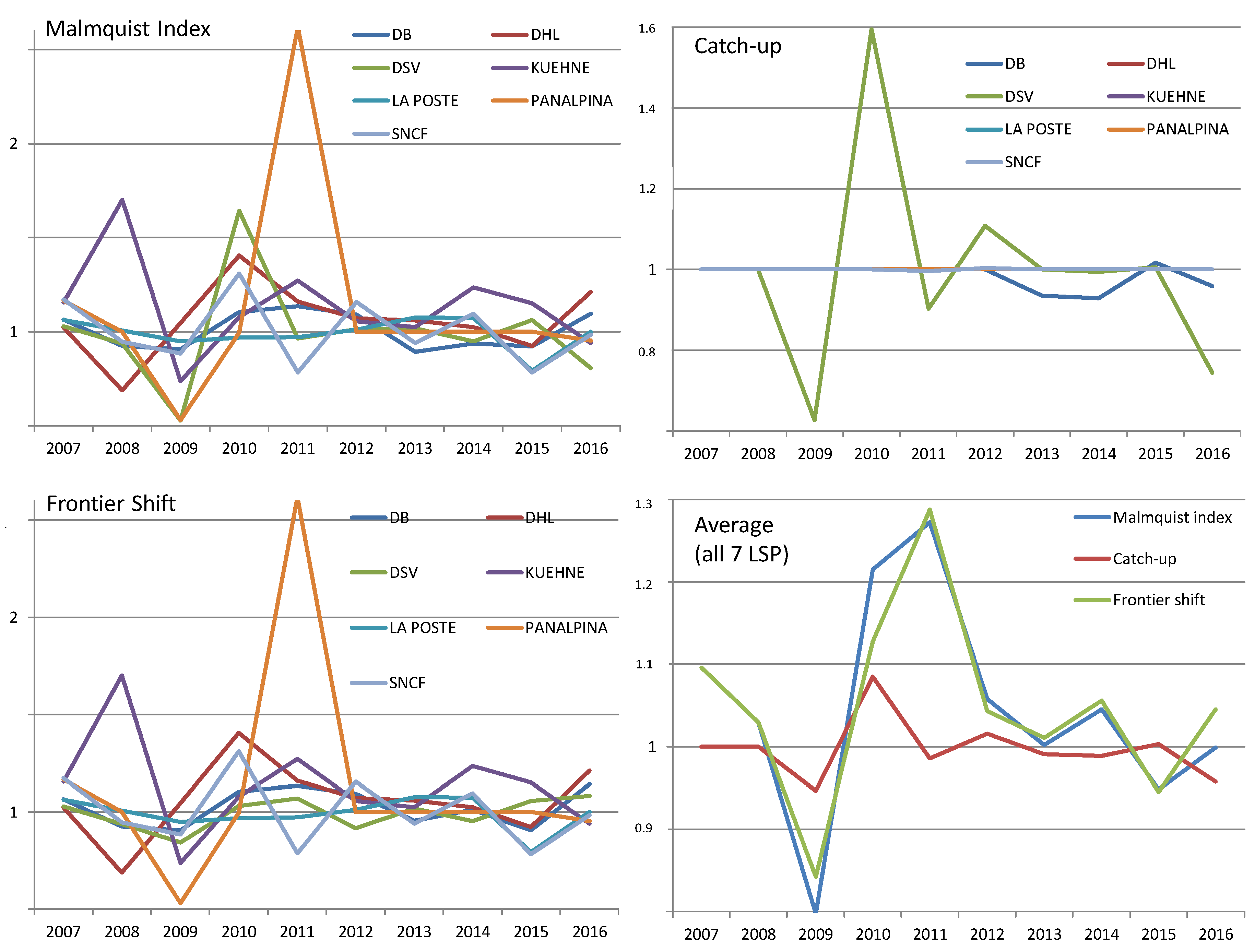
Figure 3 below for analysis and discussion.
Four different settings are reported. In the left upper corner, the aggregate development of the DEA Malmquist index is shown for all seven LSP individually. In the upper right corner, only the catch-up development as part of the Malmquist index is depicted. Whereas in the lower left corner, the frontier shift development is depicted for all seven LSP; and finally, in the lower right corner, the average development for all three index parts is characterized. As can be recognized, the total DEA Malmquist index development is mainly influenced by the frontier shift development. Catch-up developments (red line in the fourth quadrant) do play only a minor role, e.g., in the years 2008 and 2010. Also, it can be seen that smaller LSP like Panalpina or Kuehne + Nagel experience a more dynamic efficiency development compared to larger companies like DB, DHL or SNCF.

4. Discussion

In an in-depth discussion regarding the calculation results, the following items are interesting:
(A) Results single out four out of seven LSP as efficient throughout the timeline of 2006 to 2016. Three on the other hand—DB, DSV and SNCF—are experiencing inefficiencies at least in one year during this period. This is remarkable: Even though 50% of weighting restrictions are scaled as “free float” within the relative DEA method, those three LSP are not able to execute an efficient operation compared to the other LSP at least regarding one indicator from the triple bottom line. Usually, it can be expected within a DEA calculation that with seven input and output indicators almost all calculation results are reaching efficient scores—even more so as a variable returns to scale BCC model was applied.
(B) More interesting and the focus of this research is the longitudinal efficiency development over time (see e.g., Figure 3). Again, whereas DSV, DB Schenker and partly SNCF (2011/2012) are experiencing inefficiencies and therefore are “occupied” with catch-up developments (upper right graph in Figure 3), the other four LSP are actively pushing the efficiency frontier (lower left graph), e.g., Panalpina (2011) or Kuehne + Nagel in the year 2008 due to a very resilient economic posture in spite of the global economic downturn during these years. Those two “sides of the coin” are adding up to the overall Malmquist index development perspective (upper left graph) where it can be recognized that comprehensive sustainability efficiency development in a triple bottom line perspective is more or less a “wobbly triangle” challenge: Obviously, for each LSP and business year different tendencies occur and no single LSP is able to sustain efficiency improvements throughout all 11 years.
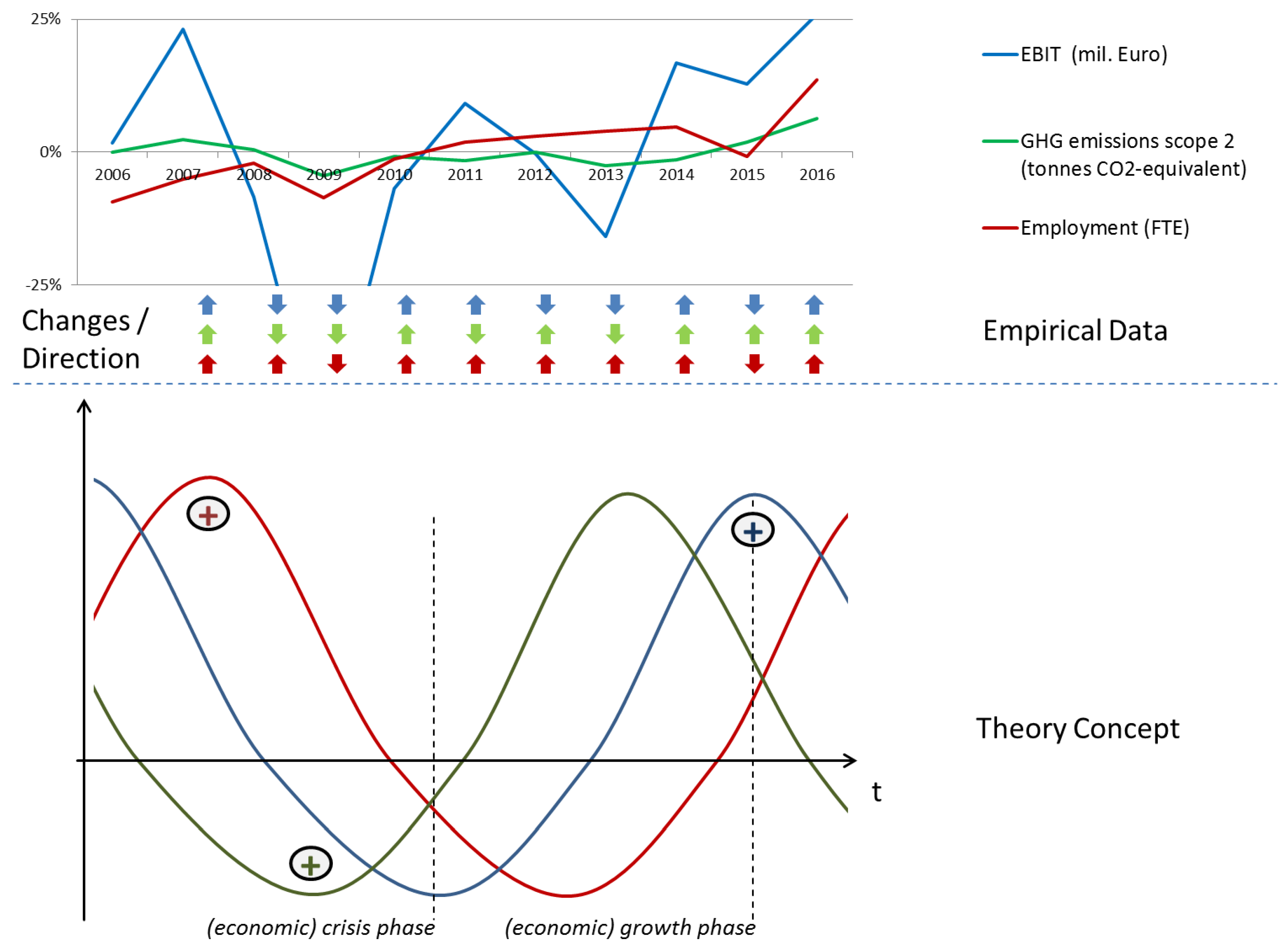
On the contrary, each and every LSP is experiencing at least one year of efficiency losses according to this TBL longitudinal calculation. This can be connected to the standard business cycle and consolidated into a further hypothesis as the proposition of a “triple separation business cycle” model. This implies as outlined in the following Figure 4 the typical growth and crisis phases of a business cycle (lower theory part)—where economic, environmental and social indicators move in accordance but with a time-lag: For example, compared to the economic business cycle of boom and bust (e.g., boom before 2007 and after 2012; bust during 2008 to 2011) the social indicator of employment is shifted to the future by about 1–2 years. For example, the peak of employment (social) is not at the same time as the peak of revenues and profit (economic) but caused by employment and dismissal restrictions for employers significantly later. For the empirical data timeline, the upper part of Figure 4 displays the deviation for each business year from the company 11-year-average values (for all 7 LSP). For example, employment shows a continuing rise with severe downturns (2009, 2015)—with the interesting year 2008 where employment still rose though the economic indicator EBIT already was falling significantly (time-lag phenomenon).
A similar picture emerges regarding the environmental factor – but with an adverse time-lag: In this case, it is theorized that economic developments experience a time-lag compared to environmental indicators like GHG emissions: Already in the first cooling phases of an economic cycle, transportation volumes are reduced significantly as e.g., stock levels are not replenished in full in anticipation of an oncoming crisis. This can be recognized in the empirical dataset for example in the year 2011, where GHG emissions already fell but EBIT only moved down one year later. Therefore, it is proposed in theory for further empirical evaluation, that the triple bottom line split business cycle for LSP contains a time-lag separation where environmental objectives and indicators are followed by economic by about 6–18 months and they again are followed by social indicators like employment by another 6–18 months. Therefore, it is highly understandable that LSP company management has a hard challenge in maintaining efficiency increases due to diverging time-lag developments of the three objective areas of environmental, economic and social indicators—obvious graphically in the change arrows depicted in the middle line of Figure 4, where there are only 5 out of 10 years with all three objective areas falling “in line” (identical upward/downward movement).
(C) In a qualitative evaluation of the selected sustainability indicators and data it may be outlined that though some applied indicators as e.g., the use of revenue as input indicator or employment as an output indicator may be counter-intuitive, the specific production theory context in a sustainability evaluation can be argued to be different from standard input-output economic analysis frameworks. Therefore, the use of assets as well as revenue as a form of corporate size in terms of input is legitimate. For output measures, the economic indicators of EBIT and dividend volume are to be judged viable as results show too. The environmental indicator of scope 2 GHG emissions has proven to be of interest in terms of efficiency development over time. But the severe disadvantage has to be highlighted that scope 2 only reports corporate direct and indirect emissions but not emissions by suppliers and subcontractors—therefore especially for LSP with different business structures wield a very high bias influence: For example, whereas DB and SNCF operate their own electricity power plants (or DHL owns a cargo aircraft fleet) and therefore report comparatively high levels of scope 2 GHG emissions, smaller LSL like Kuehne + Nagel or Panalpina do not employ own assets but only subcontractors and therefore experience significantly lower levels of scope 2 GHG emissions. Sensible comparative figures are only to expect with full disclosure of scope 3 GHG emissions throughout the whole supply chain—but these are hard to obtain throughout the multi-level subcontractor structures in logistics and time will show if they are actually publicly presented e.g., in business reports in the future. Special emphasis can be put on the innovative role of employment indicators, used in this analysis as social output performance area. Though historically viewed predominantly as input factor, in the light of the social sustainability dimension as well as the major importance in the economics and political arena in our societies, it is legitimate to re-evaluate this narrow view. Whereas personnel and especially personnel expenses are possibly used as input measures, it could be established within the social dimension of the sustainability triple bottom line that FTE quantities are also a reliable output measure for the social performance and positive impact of any corporation as suggested here for logistics.
(D) As indicated with the presentation of results in the previous section, the role of government ownership is to be discussed critically: Two fully government-owned corporations (DB in Germany and SNCF in France) are reported to have less-than efficient operations even with the indications of “decreasing returns to scale” (indicating that scaling down their business volume would actually increase overall efficiency). From the results presented here, a new angle of efficiency as a pure corporate management question can be added: As government institutions and corporations tend to grow without the “taming influence of market and competition,” it is highly likely that optimal business volume sizes are ignored and growth is sustained beyond optimal efficiency levels. Therefore, it can be argued that government ownership in private markets is not only unfair and illegal as well as destructive in a competitive market perspective but also highly inefficient and therefore prohibiting markets from providing efficient solutions for customers. This domain of government ownership and influence is a highly important question in most logistics markets, especially in Europe but also in Asia. Further research inquiries as well as political and legal discussions are warranted from the results presented here for the LSP DB (Schenker) and SNCF from Germany and France.
(E) Additionally, even accepting the limited influence of LSP towards the overall setup of global supply chains (e.g., the trend towards longer transportation distances due to sourcing, production and retail sites farther apart), on a strategic long-term level there may be a further problem: As described by Jevons in 1865 [56] and subsequently e.g., by Sorrell [187], the so-called “rebound effect” can lead to a situation with increased sustainability efficiency but in turn also with an increased use of transportation resources due to that increased efficiency (and e.g., reduced prices). This again can lead to an aggregate absolute increase in negative sustainability impacts e.g., emissions. For transportation in general, this is for example outlined by Wang and Lu [188], Winebrake et al. [189] or Matos and Silva [190]. In the analysed business reports, this is present for example with the following citation: “For example, by using dedicated freight aircraft, versus utilizing belly cargo in passenger planes, greenhouse gas emissions per ton-km of cargo can be reduced.” [171] (p. 59). This highlights that corporate objectives are usually directed at an increase of size-normalized efficiency (e.g., GHG emissions per ton-kilometre), not a reduction of overall emission or other political objectives.
(F) One overall method and management science aspect may also be added to the discussion items herein: As shown in Figure 3, the overall efficiency development for the analysed LSP is mainly influenced by the frontier shift development within the DEA Malmquist index analysis. And this frontier shift development itself again is strongly linked to the recognizable business cycle e.g., during the 2008–2010 business crisis and the recovering phase thereafter. This leads the author to postulate an interesting research hypothesis: ‘Efficiency development for individual and aggregate LSP—at least in a comprehensive triple bottom line perspective—is not only influenced by catch-up and (technical) frontier shift developments but also by a business cycle frontier shift’.
This hypothesis can be explained as an additional influencing factor with a power similar to technical developments for LSP business development: For example, oil prices act as a severe cost factor in line with business cycle developments, e.g., rising in boom times and therefore increasing the cost of all transportation accordingly and unavoidable for all logistics actors. The same is true for freight rates regarding all transport modes, sporting high volatilities during the business cycle. This can be compared to a high volatility in the technical production function, e.g., available production machinery or technical process and product blueprints. The nature of this third element as a “business cycle efficiency frontier shift” is similar to a pure technical frontier shift as all LSP are affected similarly, though some may cope with changes like oil price or freight rate changes better than others. This again is similar to the ability of individual corporations to adapt to technical changes e.g., in production technology or knowledge development. This new three-pronged efficiency development model would call for further research as well as a proposition for a new DEA efficiency index calculation providing detailed information about the actual split between the three areas regarding overall LSP efficiency. This is necessitated for overall supply chain sustainability optimization due to the central role of LSP designing and steering global supply chains.

5. Simulation

A simulation is added as complementary element to the presented research primarily in order to show implications and sensitivity perspectives regarding the proposed influences on LSP and supply chain sustainability in the TBL evaluation with regard to the business cycle. The primary results and elements outlined here are a first step and work in progress and the final simulation should incorporate real life business data in order to verify the concept of a three-factor efficiency frontier shift in a dynamic TBL evaluation setting.
In addition, the model sketch shall also outline at this stage, if an approach with three influencing factors in LSP TBL efficiency evaluation in relation to the general business cycle is applicable. This is important as guiding light for further research and shall enable an informed concept and choice for further research, i.e. if the notion of three factors in dynamic production frontier shifts are viable.
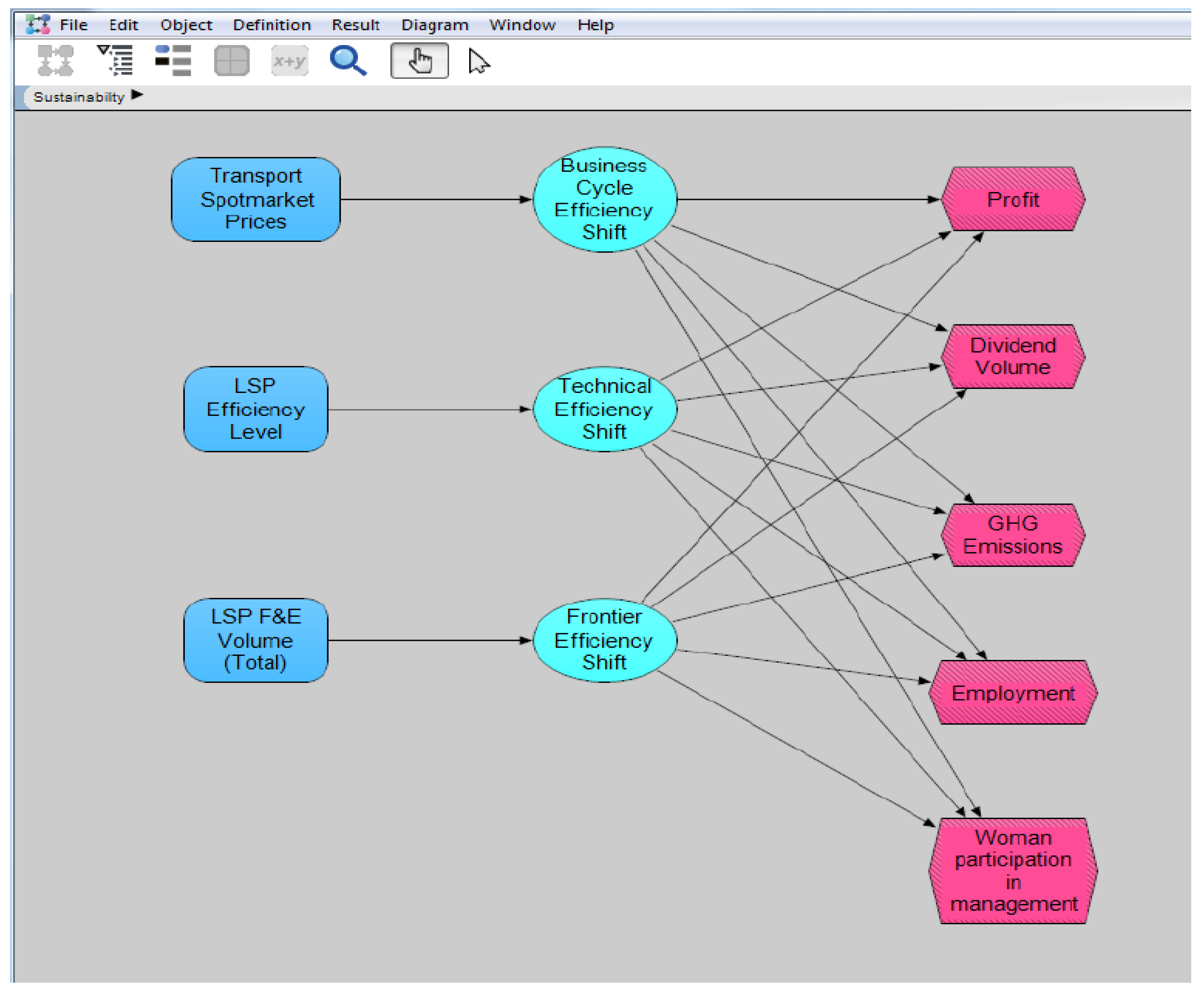
Derived from the above research results, a system dynamics simulation is applied using Analytica. The following variables and nodes are included into the model (Figure 5):
  • Objective function variables (five output parameters presented here, right side in Figure 5),
  • Transport market spot prices as input variable (start value),
  • Business cycle efficiency shift node (cycle variable with a TBL-specific time lag or off-shift between +1 and −1 one years; business cycle length of 8 years altogether),
  • LSP efficiency level as starting input variable,
  • Technical efficiency node (non-linear advance, probability function ranging from −5 to +10% per annum),
  • LSP R&D volume as input variable for efficiency frontier shift,
  • Frontier efficiency shift node (gradual advance, probability function in the range of 0 to 5% increase per annum).
This model is simulating the varying output results regarding the established TBL LSP perspective—without taking into account input volumes and therefore efficiency questions at this early stage; further research shall enlarge that to efficiency analytics simulation too.
Data is acquired at this early stage of model development from heuristics and probability functions, no real data values are included. This is planned for further stages of the simulation model in further research endeavours and studies.

6. Conclusions

In line with the important claim of rigor and relevance by Mentzer [191], this paper has pointed at the research gap of missing longitudinal calculation results for a triple bottom line sustainability efficiency of logistics service providers. Rigorous method application with the DEA Malmquist index has led to research results which are at the same time relevant for business practice and the improvement of theoretical frameworks for logistics and supply chain management, e.g., the concept of a triple bottom line split business cycle with time-lags and a business cycle frontier shift in efficiency development.
Some results and conclusions are highlighted as follows: (i) The initial research question can be answered positive: Presented results show that the DEA Malmquist index application is feasible for LSP in a longitudinal sustainability efficiency evaluation regarding triple bottom line objectives and yields interesting results; (ii) Further of interest is the fact that medium-sized LSP like Kühne + Nagel as well as Panalpina came out as efficiency leaders in such a triple bottom line sustainability evaluation—besides larger players like DHL and La Poste. It can be concluded that there is a level playing field between larger and medium-sized LSP at least in a TBL sustainability perspective; (iii) In the longitudinal perspective it is recognizable that all LSP struggle to keep up sustained positive improvements in comprehensive sustainability efficiency—this led to the suggestion of a triple bottom line split business cycle model where social development lags behind and environmental development precedes economic development indicators for LSP within the business cycle; (iv) The suggested indicators like for example employment for the social dimension of the triple bottom line are found to be very interesting as especially in a traditional efficiency and production analysis setting such indicators would usually be used as input types—but are employed here as output type.
The discussion connected to this question should be continued also regarding the further exploration towards a deeper and richer social dimension of the triple bottom line for LSP as for example suggested by Wieland, Handfield and Durach [192]. (v) The established indicators within this DEA Malmquist index calculation – asset and revenue volume as input types as well as EBIT, dividend, GHG emissions, employment and women participation in management as output types—have been proven to be relevant and meaningful for management science research regarding LSP. Other research projects should connect to these results and further the discussion regarding appropriate TBL sustainability indicators: This could for example be connected to a prior PESTLE analysis as suggested by Iacovidou et al. [193]. Also, further trends and developments in the logistics and supply chain management domain (see Fawcett and Waller [194] or Brockhaus, Kersten and Knemeyer [195]) would have to be connected to the efficiency developments of European LSP in a comprehensive sustainability setting; (vi) Method-wise it is suggested that LSP efficiency development could be best analysed by incorporating an index component business cycle frontier shift besides existing technical frontier shift and catch-up index elements.
The limitations of this study especially encompass (i) first the questions of a limited number of only seven included LSP—further studies are warranted to overcome this small sample size but keeping in mind the required comprehensive dataset from public records, usually limiting the sample severely; (ii) Second, it has to be reported that the applied output indicators are only limited to five indicators across the three TBL fields. Therefore, also extensions regarding a larger number of output indicators are necessary to replicate the results of this study further.
For the future, the following research paths could emerge from this research regarding a longitudinal sustainability efficiency evaluation of LSP. First, the proposed “triple bottom line split business cycle” regarding the three TBL line perspectives during a typical business cycle should be tested and verified further. Second, the important influencing factors of corporate size, asset strategy as well as government ownership and influence would have to be scrutinized in connected research endeavours. It would be interesting which aspects contribute most to LSP inefficiencies in a sustainability efficiency analysis. Third, it could be of interest to analyse the proposed “shaky development” further, e.g., if this holds for LSP seated in other world regions as well as during other business cycle times than the timeframe 2006 to 2016 analysed. And further confirmatory research with a larger number of LSP included would be important for advancing management science knowledge for sustainability management with LSP. Finally, as indicated in the introduction, the future evaluation and discussion of sustainability performance by LSP should be considered paramount to sustainability management in general as in a time of global supply chains, LSP are a central cornerstone of any value chain for any given product in worldwide markets.
Relevance for business practice is provided in the perspective of real-world data from LSP applied and the specific contribution in suggesting an efficiency design framework for sustainable supply chains. Therefore, individual forwarders are able to align their key performance indicator (KPI) setup and framework with the TBL indicators outlined and analysed here, as well as being aware of the fact that efficiency improvement might not be that easy due to the described efficiency upward and downwards drags during the business cycle—known from the general economic and transport environment (e.g., volatile transport volumes) but shown here for sustainability TBL indicators. This is connected to the framework of sustainable supply chains [37] as well as functional contributions to sustainability from different fields like manufacturing, packaging and operations within the reach of LSP in the supply chain as exemplified by Turki et al. [196] or Carter and Easton [197].
Therefore, it is an important responsibility of forwarders to cater to the needs of human and global sustainability development. Sustainability and efficiency can be seen as cousins—indicating a relationship but not a very strong one. Indicating also, that there can be positive close contact and common objectives (e.g., if economic efficiency supports employment objectives in the social dimension). But there can also be negative distance and divergence of objectives, e.g., if increasing economic activity fosters economic success and sustainability but hinders environmental sustainability by increasing emissions and resource use. This is for example highlighted and discussed by a growing part of research literature as e.g., mentioned by García-Arca et al. [198], Carter and Rogers [199], Mejías et al. [5] or Andersen and Skjoett-Larsen [200]—sustainability and efficiency do not need to be enemies but can work together and help each other. It is the task and art of successful management (Drucker [201]) to lead sustainability and efficiency into the positive and mutually supportive direction with professional and research-based supply chain management.

Conflicts of Interest

The author declares no conflict of interest.

References

  1. Eurostat. Greenhouse Gas Emissions–Analysis per Source Sector. Eurostat LuxembourgEurostat. 2017. Available online: http://ec.europa.eu/eurostat/statistics-explained/index.php/File:Greenhouse_gas_emissions,analysis_by_source_sector,_EU-28,_1990_and_2015_(percentage_of_total)_new.png (accessed on 30 November 2017).
  2. Vachon, S.; Klassen, R.D. Extending green practices across the supply chain: The impact of upstream and downstream integration. Int. J. Oper. Prod. Manag. 2006, 26, 795–821. [Google Scholar] [CrossRef]
  3. Halldórsson, A.; Kovács, G. The sustainable agenda and energy efficiency: Logistics solutions and supply chains in times of climate change. Int. J. Phys. Distrib. Logist. Manag. 2010, 40, 5–13. [Google Scholar] [CrossRef]
  4. McKinnon, A.; Browne, M.; Whiteing, A.; Piecyk, M. Green Logistics: Improving the Environmental Sustainability of Logistics; Kogan Page: London, UK, 2015; ISBN 978-0749456788. [Google Scholar]
  5. Mejías, A.M.; Paz, E.; Pardo, J.E. Efficiency and sustainability through the best practices in the Logistics Social Responsibility framework. Int. J. Phys. Distrib. Logist. Manag. 2016, 36, 164–199. [Google Scholar] [CrossRef]
  6. Golinska-Dawson, P.; Kolinski, A. Efficiency in Sustainable Supply Chain; Springer: Cham, Switzerland, 2017; ISBN 978-3319464503. [Google Scholar]
  7. Sudarto, S.; Takahashi, K.; Morikawa, K. Efficient flexible long-term capacity planning for optimal sustainability dimensions performance of reverse logistics social responsibility: A system dynamics approach. Int. J. Prod. Econ. 2016, 184, 179–192. [Google Scholar] [CrossRef]
  8. Ma, K.; Wang, L.; Chen, Y. A collaborative cloud service platform for realizing sustainable make-to-order apparel supply chain. Sustainability 2018, 10, 11. [Google Scholar] [CrossRef]
  9. Tang, A.K.Y.; Lai, K.-H.; Cheng, T.C.E. A Multi-research-method approach to studying environmental sustainability in retail operations. Int. J. Prod. Econ. 2016, 171, 394–404. [Google Scholar] [CrossRef]
  10. Lucato, W.C.; da Silva Santo, J.C.; Pacchini, A.P.T. Measuring the sustainability of manufacturing process: A conceptual framework. Sustainability 2018, 10, 81. [Google Scholar] [CrossRef]
  11. Dijkema, G.P.J.; Ferra, P.; Herder, P.M.; Heitor, M. Trends and opportunities framing innovation for sustainability in the learning society. Technol. Forecast. Soc. Chang. 2006, 73, 215–227. [Google Scholar] [CrossRef]
  12. Heiskala, M.; Jokinen, J.-P.; Tinnilä, M. Crowdsensing-based transportation services–An analysis from business model and sustainability viewpoints. Res. Transp. Bus. Manag. 2016, 18, 38–48. [Google Scholar] [CrossRef]
  13. Rimos, S.; Hoadley, A.F.A.; Brennan, D.J. Environmental consequence analysis for resource depletion. Proc. Saf. Environ. Prot. 2014, 9, 849–861. [Google Scholar] [CrossRef]
  14. Kuhn, M.A.; Kuhn, P.; Villeval, M.C. Decision-Environment Effects on Intertemporal Financial Choices: How Relevant are Resource-Depletion Models? J. Econ. Behav. Organ. 2017, 137, 72–89. [Google Scholar] [CrossRef]
  15. Mahoney, L.S.; Thorne, L.; Cecil, L.; LaGore, W. A research note on standalone corporate social responsibility reports: Signaling or greenwashing? Crit. Perspect. Account. 2013, 24, 350–359. [Google Scholar] [CrossRef]
  16. Siano, A.; Vollero, A.; Conte, F.; Amabile, S. ‘More than words’: Expanding the taxonomy of greenwashing after the Volkswagen scandal. J. Bus. Res. 2017, 71, 27–37. [Google Scholar] [CrossRef]
  17. Brix-Asala, C.; Hahn, R.; Seuring, S. Reverse logistics and informal valorisation at the Base of the Pyramid: A case study on sustainability synergies and trade-offs. Eur. Manag. J. 2016, 34, 414–423. [Google Scholar] [CrossRef]
  18. Davarzani, H.; Fahimnia, B.; Bell, M.; Sarkis, J. Greening ports and maritime logistics: A review. Transp. Res. Part D 2016, 48, 473–487. [Google Scholar] [CrossRef]
  19. Osorio-Tejada, J.L.; Llera-Sastresa, E.; Scarpellini, S. A multi-criteria sustainability assessment for biodiesel and liquefied natural gas as alternative fuels in transport systems. J. Natl. Gas Sci. Eng. 2017, 42, 169–186. [Google Scholar] [CrossRef]
  20. Armeanu, D.S.; Vintila, G.; Gherghina, S.C. Empirical study towards the drivers of sustainable aconomic growth in EU-28 countries. Sustainability 2018, 10, 4. [Google Scholar] [CrossRef]
  21. United Nations Framework Convention on Climate Change (UNFCCC). United Nations Framework Convention on Climate Change; Climate Change Secretariat: Bonn, Germany, 1992. [Google Scholar]
  22. United Nations Framework Convention on Climate Change (UNFCCC). Kyoto Protocol; Climate Change Secretariat: Bonn, Germany, 1998. [Google Scholar]
  23. United Nations Framework Convention on Climate Change (UNFCCC). Copenhagen Accord 2009; Climate Change Secretariat: Bonn, Germany, 2009. [Google Scholar]
  24. United Nations Framework Convention on Climate Change (UNFCCC). Doha Amendment to the Kyoto Protocol 2012; Climate Change Secretariat: Bonn, Germany, 2012. [Google Scholar]
  25. United Nations Framework Convention on Climate Change (UNFCCC). Paris Agreement 2015; Climate Change Secretariat: Bonn, Germany, 2015. [Google Scholar]
  26. Brundtlandt, G.M. Our Common Future; World Commission on Environment and Development: New York, NY, USA, 1988. [Google Scholar]
  27. Holden, E.; Linnerud, K.; Banister, D. Sustainable development: Our Common Future revisited. Glob. Environ. Chang. 2014, 26, 130–139. [Google Scholar] [CrossRef]
  28. Sneddon, C.; Howarth, R.B.; Norgaard, R.B. Sustainable development in a post-Brundtland world. Ecol. Econom. 2006, 57, 253–268. [Google Scholar] [CrossRef]
  29. Von Carlowitz, H.-C. Sylvicultura Oeconomica; J.F. Braun: Leipzig, Germany, 1713. [Google Scholar]
  30. Meadows, D.H.; Meadows, D.L.; Randers, J.; Behrens, W.W. The Limits to Growth; Universe Books: New York, NY, USA, 1972; ISBN 978-1849775861. [Google Scholar]
  31. Vermeulen, W.J.V.; Witjes, S. On addressing the dual and embedded nature of business and the route towards corporate sustainability. J. Clean. Prod. 2016, 112, 2822–2832. [Google Scholar] [CrossRef]
  32. Brockhaus, S.; Fawcett, S.E.; Knemeyer, A.M.; Fawcett, A.M. Motivations for environmental and social consciousness: Reevaluating the sustainability-based view. J. Clean. Prod. 2017, 143, 933–947. [Google Scholar] [CrossRef]
  33. McManners, P.J. Developing policy integrating sustainability: A case study into aviation. Environ. Sci. Policy 2016, 57, 86–92. [Google Scholar] [CrossRef]
  34. Chang, R.-D.; Zuo, J.; Zhao, Z.-Y.; Zillante, G.; Gan, X.-L.; Soebarto, V. Evolving theories of sustainability and firms: History, future directions and implications for renewable energy research. Renew. Sustain. Energy Rev. 2017, 72, 48–56. [Google Scholar] [CrossRef]
  35. Centobelli, P.; Cerchione, R.; Esposito, E. Environmental sustainability in the service industry of transportation and logistics service providers: Systematic literature review and research directions. Trans. Res. Part D Trans. Environ. 2017, 53, 454–470. [Google Scholar] [CrossRef]
  36. Schrettle, S.; Hinz, A.; Scherrer-Rathje, M.; Friedli, T. Turning sustainability into action: Explaining firms’ sustainability efforts and their impact on firm performance. Int. J. Prod. Econ. 2014, 147, 73–84. [Google Scholar] [CrossRef]
  37. Seuring, S.; Müller, M. From a literature review to a conceptual framework for sustainable supply chain management. J Clean. Prod. 2008, 16, 1699–1710. [Google Scholar] [CrossRef]
  38. Fahimnia, B.; Jabbarzadeh, A. Marrying supply chain sustainability and resilience: A match made in heaven. Trans. Res. Part E 2016, 91, 306–324. [Google Scholar] [CrossRef]
  39. Kaur, H.; Singh, S.P. Heuristic modeling for sustainable procurement and logistics in a supply chain using big data. Comput. Oper. Res. 2017. [Google Scholar] [CrossRef]
  40. Suzuki, Y.; Lu, S.-H. Economies of product diversity in collaborative logistics. J. Bus. Logist. 2017, 38, 115–129. [Google Scholar] [CrossRef]
  41. Evangelista, P.; Colicchia, C.; Creazza, A. Is environmental sustainability a strategic priority for logistics service providers? J. Environ. Manag. 2017, 198, 353–362. [Google Scholar] [CrossRef] [PubMed]
  42. Colicchia, C.; Marchet, G.; Melacini, M.; Perotti, S. Building environmental sustainability: Empirical evidence from Logistics Service Providers. J Clean. Prod. 2013, 59, 197–209. [Google Scholar] [CrossRef]
  43. Sim, J.; Sim, J. Air emission and environmental impact assessment of Korean automotive logistics. J. Clean. Prod. 2017, 159, 130–140. [Google Scholar] [CrossRef]
  44. European Environmental Agency (EEA). Greenhouse Gas Emissions from Transport; EEA: Copenhagen, Denmark, 2017; Available online: https://www.eea.europa.eu/data-and-maps/indicators/transport-emissions-of-greenhouse-gases/transport-emissions-of-greenhouse-gases-10 (accessed on 30 January 2018).
  45. Levallois, C. Can de-growth be considered a policy option? A historical note on Nicholas Georgescu-Roegen and the Club of Rome. Ecol. Econ. 2010, 69, 2271–2278. [Google Scholar] [CrossRef]
  46. European Commission. Roadmap to a Single European Transport Area–Towards a Competitive and Resource Efficient Transport System; European Commission: Brussels, Germany, 2011; COM(2011)144 final. [Google Scholar]
  47. Du, T. Performance measurement of healthcare service and association discussion between quality and efficiency: Evidence from 31 provinces of mainland china. Sustainability 2018, 10, 74. [Google Scholar] [CrossRef]
  48. Mohanty, M.; Shankar, R. Modelling uncertainty in sustainable integrated logistics using Fuzzy-TISM. Transp. Res. Part D 2017, 53, 471–491. [Google Scholar] [CrossRef]
  49. Marshall, D.; McCarthy, L.; McGrath, P.; Claudy, M. Going above and beyond: How sustainability culture and entrepreneurial orientation drive social sustainability supply chain practice adoption. Supply Chain Manag. Int. J. 2015, 20, 434–454. [Google Scholar] [CrossRef]
  50. Deutsche Bahn. 2016 Integrated Report-Quality That Persuades! Deutsche Bahn AG: Berlin, Germany, 2017. [Google Scholar]
  51. Deutsche Post DHL. Smart Logistics–2015 Annual Report; Deutsche Post AG: Bonn, Germany, 2016. [Google Scholar]
  52. Gammelgaard, B.; Andersen, C.B.G.; Aastrup, J. Value co-creation in the interface between city logistics provider and in-store processes. Trans. Res. Proc. 2016, 12, 787–799. [Google Scholar] [CrossRef]
  53. Oltean-Dumbrava, C.; Watts, G.; Miah, A. Towards a more sustainable surface transport infrastructure: A case study of applying multi criteria analysis techniques to assess the sustainability of transport noise reducing devices. J. Clean. Prod. 2016, 112, 2922–2934. [Google Scholar] [CrossRef]
  54. Postorino, M.N.; Mantecchini, L. A transport carbon footprint methodology to assess airport carbon emissions. J. Air Trans. Manag. 2014, 37, 76–86. [Google Scholar] [CrossRef]
  55. Gupta, M.D. Carbon footprint from road transport use in Kolkata city. Trans. Res. Part D 2014, 32, 397–410. [Google Scholar] [CrossRef]
  56. Jevons, W.S. The Coal Question: An Inquiry Concerning the Progress of the Nation, and the Probable Exhaustion of Our Coal Mines; Macmillan: London, UK, 1865. [Google Scholar]
  57. Alcott, B. Jevons’ paradox. Ecol. Econ. 2005, 54, 9–21. [Google Scholar] [CrossRef]
  58. Higgins, C.; Coffey, B. Improving how sustainability reports drive change: A critical discourse analysis. J. Clean. Prod. 2016, 136, 18–29. [Google Scholar] [CrossRef]
  59. Domingues, A.R.; Lozano, R.; Ceulemanns, K.; Ramos, T.B. Sustainability reporting in public sector organisations: Exploring the relation between the reporting process and organisational change management for sustainability. J. Environ. Manag. 2017, 192, 292–301. [Google Scholar] [CrossRef] [PubMed]
  60. Eroglu, C.; Kurt, A.C.; Elwakil, O.S. Stock market reaction to quality, safety, and sustainability awards in logistics. J. Bus. Logist. 2016, 37, 329–345. [Google Scholar] [CrossRef]
  61. Ha, H.K.; Kaneko, S.; Yamamoto, M.; Yoshida, Y.; Zhang, A. On the discrepancy in the social efficiency measures between parametric and non-parametric production technology identification. J. Air Trans. Manag. 2017, 58, 9–14. [Google Scholar] [CrossRef]
  62. Toma, P.; Miglietta, P.P.; Zurlini, G.; Valente, D.; Petrosillo, I. A non-parametric bootstrap data envelopment analysis approach for environmental policy planning and management of agricultural efficiency in EU countries. Ecol. Indic. 2017, 83, 132–143. [Google Scholar] [CrossRef]
  63. Chen, C.-M. A critique of non-parametric efficiency analysis in energy economics studies. Energy Econ. 2013, 28, 146–152. [Google Scholar] [CrossRef]
  64. Koopmans, T.C. Analysis of Production as an Efficient Combination of Activities. In Activity Analysis of Production and Allocation, Proceedings of a Conference; Koopmans, T.C., Ed.; Wiley: New York, NY, USA, 1951; pp. 33–97. [Google Scholar]
  65. Debreu, G. The Coefficient of Resource Utilization. Econometrica 1951, 19, 273–292. [Google Scholar] [CrossRef]
  66. Farrell, M.J. The Measurement of Productive Efficiency. J. R. Stat. Soc. Ser. A (Gen.) 1957, 120, 253–290. [Google Scholar] [CrossRef]
  67. Diewert, W.E. Functional Forms for Profit and Transformation Functions. J. Econ. Theory 1973, 6, 284–316. [Google Scholar] [CrossRef]
  68. Charnes, A.; Cooper, W.W.; Rhodes, E.L. Measuring the efficiency of decision making units. Eur. J. Oper. Res. 1978, 2, 429–444. [Google Scholar] [CrossRef]
  69. Karsak, E.E.; Karadayi, M.A. Imprecise DEA framework for evaluating health care performance of districts. Kybernetes 2017, 46. [Google Scholar] [CrossRef]
  70. Shwartz, M.; Burgess, J.F.; Zhu, J. A DEA based composite measure of quality and its associated data uncertainty interval for health care provider profiling and pay-for-performance. Eur. J. Oper. Res. 2016, 253, 489–502. [Google Scholar] [CrossRef]
  71. Hollingsworth, B. Non-Parametric and Parametric Applications Measuring Efficiency in Health Care. Health Care Manag. Sci. 2003, 6, 203–218. [Google Scholar] [CrossRef] [PubMed]
  72. Bolli, T.; Olivares, M.; Bonaccorsi, A.; Daraio, C.; Aracil, A.D.; Lepori, B. The differential effects of competitive funding on the production frontier and the efficiency of universities. Econ. Educ. Rev. 2016, 52, 91–104. [Google Scholar] [CrossRef]
  73. Bessent, A.M.; Bessent, E.W.; Charnes, A.; Cooper, W.W.; Thorogood, N. Evaluation of educational program proposals by means of DEA. Educ. Adm. Q. 1983, 19, 82–107. [Google Scholar] [CrossRef]
  74. Banker, R.D.; Charnes, A.; Cooper, W.W. Some models for estimating technical and scale inefficiencies in data envelopment analysis. Manag. Sci. 1984, 30, 1078–1092. [Google Scholar] [CrossRef]
  75. Malmquist, S. Index numbers and indifference surfaces. Trab. Estad. Investig. Oper. 1953, 42, 209–242. [Google Scholar] [CrossRef]
  76. Caves, D.W.; Christensen, L.R.; Diewert, W. The Economic Theory of Index Numbers and the Measurement of Input, Output, and Productivity. Econometrica 1982, 50, 1393–1414. [Google Scholar] [CrossRef]
  77. Grifell-Tatje, E.; Lovell, C.A.K.; Pastor, J.T. A quasi-Malmquist productivity index. J. Product. Anal. 1998, 10, 7–20. [Google Scholar] [CrossRef]
  78. Thanassoulis, E.; Shiraz, R.K.; Maniadakis, N. A cost Malmquist productivity index capturing group performance. Eur. J. Oper. Res. 2015, 241, 796–805. [Google Scholar] [CrossRef]
  79. Emrouznejad, A.; Yang, G. A framework for measuring global Malmquist-Luenberger productivity index with CO2 emissions on Chinese manufacturing industries. Energy 2016, 115, 840–856. [Google Scholar] [CrossRef]
  80. Sueyoshi, T.; Goto, M. DEA environmental assessment in time horizon: Radial approach for Malmquist index measurement on petroleum companies. Energy Econ. 2015, 51, 329–345. [Google Scholar] [CrossRef]
  81. Chang, D.-S.; Kuo, L.R.; Chen, Y. Industrial changes in corporate sustainability performance–an empirical overview using data envelopment analysis. J Clean. Prod. 2013, 56, 147–155. [Google Scholar] [CrossRef]
  82. Charnes, A.; Cooper, W.W. Preface to topics in data envelopment analysis. Ann. Oper. Res. 1985, 2, 59–94. [Google Scholar] [CrossRef]
  83. Färe, R.; Grosskopf, S.; Lovell, C.A.K.; Pasurka, C. Multilateral productivity comparisons when some outputs are undesirable. Rev. Econ. Stat. 1989, 71, 90–98. [Google Scholar] [CrossRef]
  84. Guo, X.; Lu, C.-C.; Lee, J.-H.; Chiu, Y.-H. Applying the dynamic DEA model to evaluate the energy efficiency of OECD countries and China. Energy 2017, 134, 392–399. [Google Scholar] [CrossRef]
  85. Khushalani, J.; Ozcan, Y.A. Are hospitals producing quality care efficiently? An analysis using Dynamic Network Data Envelopment Analysis (DEA). Socio-Econ. Plan. Sci. 2017, 60, 15–23. [Google Scholar] [CrossRef]
  86. Vlontzos, G.; Pardalos, P.M. Assess and prognosticate green house gas emissions from agricultural production of EU countries, by implementing, DEA Window analysis and artificial neural networks. Renew. Sustain. Energy Rev. 2017, 76, 155–162. [Google Scholar] [CrossRef]
  87. Halkos, G.E.; Tzeremes, N.G. Exploring the existence of Kuznets curve in countries’ environmental efficiency using DEA window analysis. Ecol. Econ. 2009, 68, 2168–2176. [Google Scholar] [CrossRef] [Green Version]
  88. Sueyoshi, T.; Goto, M.; Sugiyama, M. DEA window analysis for environmental assessment in a dynamic time shift: Performance assessment of U.S. coal-fired power plants. Energy Econ. 2013, 40, 845–857. [Google Scholar] [CrossRef]
  89. Kazley, A.S.; Ozcan, Y.A. Electronic medical record use and efficiency: A DEA and windows analysis of hospitals. Socio-Econ. Plan. Sci. 2009, 43, 209–216. [Google Scholar] [CrossRef]
  90. Pulina, M.; Detotto, C.; Paba, A. An investigation into the relationship between size and efficiency of the Italian hospitality sector: A window DEA approach. Eur. J. Oper. Res. 2010, 204, 613–620. [Google Scholar] [CrossRef]
  91. La Poste. 2016 CSR Report; Le Groupe La Poste: Paris, France, 2017. [Google Scholar]
  92. Elkington, J. Cannibals with Forks–The Triple Bottom Line of 21st Century Business; Capstone: Oxford, UK, 1997; ISBN 978-1841120843. [Google Scholar]
  93. Formentini, M.; Taticchi, P. Corporate sustainability approaches and governance mechanisms in sustainable supply chain management. J. Clean. Prod. 2016, 112, 1920–1933. [Google Scholar] [CrossRef] [Green Version]
  94. Akhtar, P.; Tse, Y.K.; Khan, Z.; Rao-Nicholson, R. Data-driven and adaptive leadership contributing to sustainability: Global agri-food supply chains connected with emerging markets. Int. J. Prod. Econ. 2015, 181, 392–401. [Google Scholar] [CrossRef]
  95. Hansen, T.; Coenen, L. The geography of sustainability transitions: Review, synthesis and reflections on an emergent research field. Environ. Innov. Soc. Trans. 2015, 17, 92–109. [Google Scholar] [CrossRef]
  96. Luthra, S.; Garg, D.; Haleem, A. An analysis of interactions among critical success factors to implement green supply chain management towards sustainability: An Indian perspective. Resour. Policy 2015, 46, 37–50. [Google Scholar] [CrossRef]
  97. Lehtonen, M. The environmental-social interface of sustainable development: Capabilities, social capital, institutions. Ecol. Econ. 2004, 49, 199–214. [Google Scholar] [CrossRef]
  98. Grund, C. Gender pay gaps among highly educated professionals—Compensation components do matter. Lab. Econ. 2015, 34, 118–126. [Google Scholar] [CrossRef]
  99. Buchanan, T. The Influence of Gender Role Attitudes on Perceptions of Women’s Work Performance and the Importance of Fair Pay. Sociol. Spectr. 2014, 34, 203–221. [Google Scholar] [CrossRef]
  100. Al-Shaer, H.; Zaman, M. Board gender diversity and sustainability reporting quality. J. Contemp. Account. Econ. 2016, 12, 210–222. [Google Scholar] [CrossRef]
  101. Perryman, A.A.; Fernando, G.D.; Tripathy, A. Do gender differences persist? An examination of gender diversity on firm performance, risk, and executive compensation. J. Bus. Res. 2016, 69, 579–586. [Google Scholar] [CrossRef]
  102. Wang, Z.; He, W. CO2 emissions efficiency and marginal abatement costs of the regional transportation sectors in China. Trans. Res. Part D 2017, 50, 83–97. [Google Scholar] [CrossRef]
  103. Voytenko, Y.; McCormick, K.; Evans, J.; Schliwa, G. Urban living labs for sustainability and low carbon cities in Europe: Towards a research agenda. J Clean. Prod. 2016, 123, 45–54. [Google Scholar] [CrossRef]
  104. Alibeyg, A.; Contreras, I.; Fernández, E. Hub network design problems with profits. Trans. Res. Part E 2016, 96, 40–59. [Google Scholar] [CrossRef]
  105. Li, Y.; Chen, H.; Prins, C. Adaptive large neighborhood search for the pickup and delivery problem with time windows, profits, and reserved requests. Eur. J. Oper. Res. 2016, 252, 27–38. [Google Scholar] [CrossRef]
  106. OECD. OECD Data–Exchange Rates. Available online: https://data.oecd.org/conversion/exchange-rates.htm (accessed on 30 November 2017).
  107. Klumpp, M. Do forwarders improve sustainability efficiency? Evidence from a European DEA Malmquist Index Calculation. Sustainability 2017, 9, 842. [Google Scholar] [CrossRef]
  108. Deutsche Bahn. 2015 Integrated Report—More Quality, More Customers, More Success; Deutsche Bahn AG: Berlin, Germany, 2016. [Google Scholar]
  109. Deutsche Bahn. 2014 Integrated Report—Integrated Thinking. Sustainable Action. Long-Term Success; Deutsche Bahn AG: Berlin, Germany, 2015. [Google Scholar]
  110. Deutsche Bahn. 2013 Integrated Report—DB2020: Our Compass, Even in Challenging Times; Deutsche Bahn AG: Berlin, Germany, 2014. [Google Scholar]
  111. Deutsche Bahn. Our Future: Sustainably Successful—Deutsche Bahn 2012 Annual Report; Deutsche Bahn AG: Berlin, Germany, 2013. [Google Scholar]
  112. Deutsche Bahn. DB Mobility Logistics—2011 Annual Report; Deutsche Bahn AG: Berlin, Germany, 2012. [Google Scholar]
  113. Deutsche Bahn. 2010 Annual Report; Deutsche Bahn AG: Berlin, Germany, 2011. [Google Scholar]
  114. Deutsche Bahn. 2009 Annual Report; Deutsche Bahn AG: Berlin, Germany, 2010. [Google Scholar]
  115. Deutsche Bahn. 2008 Annual Report; Deutsche Bahn AG: Berlin, Germany, 2009. [Google Scholar]
  116. Deutsche Bahn. 2007 Annual Report; Deutsche Bahn AG: Berlin, Germany, 2008. [Google Scholar]
  117. Deutsche Bahn. 2006 Annual Report; Deutsche Bahn AG: Berlin, Germany, 2007. [Google Scholar]
  118. Deutsche Post DHL. 2016 Annual Report—Constantly Reinventing the Future of Logistics; Deutsche Bahn AG: Berlin, Germany, 2017. [Google Scholar]
  119. Deutsche Post DHL. When You Think of Logistics—2014 Annual Report; Deutsche Bahn AG: Berlin, Germany, 2015. [Google Scholar]
  120. Deutsche Post DHL. Tailor Made—2013 Annual Report; Deutsche Post AG: Bonn, Germany, 2014. [Google Scholar]
  121. Deutsche Post DHL. Pioneering Future Markets—2012 Annual Report; Deutsche Post AG: Bonn, Germany, 2013. [Google Scholar]
  122. Deutsche Post DHL. Simply Grow—2011 Annual Report; Deutsche Post AG: Bonn, Germany, 2012. [Google Scholar]
  123. Deutsche Post DHL. Being Your Choice—2010 Annual Report; Deutsche Post AG: Bonn, Germany, 2011. [Google Scholar]
  124. Deutsche Post DHL. Showing Respect, Delivering Results—2009 Annual Report; Deutsche Post AG: Bonn, Germany, 2010. [Google Scholar]
  125. Deutsche Post DHL. Delivering on the Future—2008 Annual Report; Deutsche Post AG: Bonn, Germany, 2009. [Google Scholar]
  126. Deutsche Post DHL. Roadmap to Value—2007 Annual Report; Deutsche Post AG: Bonn, Germany, 2008. [Google Scholar]
  127. Deutsche Post DHL. Building on Our Strategic Strengths—2006 Annual Report; Deutsche Post AG: Bonn, Germany, 2007. [Google Scholar]
  128. DSV. 2016 Annual Report; DSV A/S: Hedehusene, Denmark, 2017. [Google Scholar]
  129. DSV. 2015 Annual Report; DSV A/S: Hedehusene, Denmark, 2016. [Google Scholar]
  130. DSV. 2014 Annual Report; DSV A/S: Hedehusene, Denmark, 2015. [Google Scholar]
  131. DSV. 2013 Annual Report; DSV A/S: Hedehusene, Denmark, 2014. [Google Scholar]
  132. DSV. 2012 Annual Report; DSV A/S: Hedehusene, Denmark, 2013. [Google Scholar]
  133. DSV. 2011 Annual Report; DSV A/S: Hedehusene, Denmark, 2012. [Google Scholar]
  134. DSV. 2010 Annual Report; DSV A/S: Hedehusene, Denmark, 2011. [Google Scholar]
  135. DSV. 2009 Annual Report; DSV A/S: Hedehusene, Denmark, 2010. [Google Scholar]
  136. DSV. 2008 Annual Report; DSV A/S: Hedehusene, Denmark, 2009. [Google Scholar]
  137. DSV. 2007 Annual Report; DSV A/S: Hedehusene, Denmark, 2008. [Google Scholar]
  138. DSV. 2006 Annual Report; DSV A/S: Hedehusene, Denmark, 2007. [Google Scholar]
  139. Kuehne + Nagel. Annual Report 2016; Kuehne + Nagel: Schindellegi, Switzerland, 2017. [Google Scholar]
  140. Kuehne + Nagel. Annual Report 2015—Tradition and Innovation; Kuehne + Nagel: Schindellegi, Switzerland, 2016. [Google Scholar]
  141. Kuehne + Nagel. Annual Report 2014—Global. Customer-Oriented. Innovative; Kuehne + Nagel: Schindellegi, Switzerland, 2015. [Google Scholar]
  142. Kuehne + Nagel. Annual Report 2013—Continuity and Further Development; Kuehne + Nagel: Schindellegi, Switzerland, 2014. [Google Scholar]
  143. Kuehne + Nagel. Annual Report 2012—People. Network. Objectives; Kuehne + Nagel: Schindellegi, Switzerland, 2013. [Google Scholar]
  144. Kuehne + Nagel. Annual Report 2011—Network and Product Portfolio–Kühne + Nagel Accelerates Expansion; Kuehne + Nagel: Schindellegi, Switzerland, 2012. [Google Scholar]
  145. Kuehne + Nagel. Annual Report 2010; Kuehne + Nagel: Schindellegi, Switzerland, 2011. [Google Scholar]
  146. Kuehne + Nagel. Annual Report 2009; Kuehne + Nagel: Schindellegi, Switzerland, 2010. [Google Scholar]
  147. Kuehne + Nagel. Annual Report 2008; Kuehne + Nagel: Schindellegi, Switzerland, 2009. [Google Scholar]
  148. Kuehne + Nagel. Annual Report 2007; Kuehne + Nagel: Schindellegi, Switzerland, 2008. [Google Scholar]
  149. Kuehne + Nagel. Annual Report 2006; Kuehne + Nagel: Schindellegi, Switzerland, 2007. [Google Scholar]
  150. La Poste. Registration Document 2016; Le Groupe La Poste: Paris, France, 2017. [Google Scholar]
  151. La Poste. Registration Document 2015; Le Groupe La Poste: Paris, France, 2016. [Google Scholar]
  152. La Poste. Registration Document 2014; Le Groupe La Poste: Paris, France, 2015. [Google Scholar]
  153. La Poste. Registration Document 2013; Le Groupe La Poste: Paris, France, 2014. [Google Scholar]
  154. La Poste. Registration Document 2012; Le Groupe La Poste: Paris, France, 2013. [Google Scholar]
  155. La Poste. Registration Document 2011; Le Groupe La Poste: Paris, France, 2012. [Google Scholar]
  156. La Poste. Registration Document 2010; Le Groupe La Poste: Paris, France, 2011. [Google Scholar]
  157. La Poste. Registration Document 2009; Le Groupe La Poste: Paris, France, 2010. [Google Scholar]
  158. La Poste. Registration Document 2008; Le Groupe La Poste: Paris, France, 2009. [Google Scholar]
  159. La Poste. Registration Document 2007; Le Groupe La Poste: Paris, France, 2008. [Google Scholar]
  160. La Poste. Registration Document 2006; Le Groupe La Poste: Paris, France, 2007. [Google Scholar]
  161. Panalpina. 2016 Annual Report; Panalpina World Transport (Holding) Ltd.: Basel, Switzerland, 2017. [Google Scholar]
  162. Panalpina. 2015 Annual Report; Panalpina World Transport (Holding) Ltd.: Basel, Switzerland, 2016. [Google Scholar]
  163. Panalpina. 2014 Annual Report; Panalpina World Transport (Holding) Ltd.: Basel, Switzerland, 2015. [Google Scholar]
  164. Panalpina. 2013 Annual Report; Panalpina World Transport (Holding) Ltd.: Basel, Switzerland, 2014. [Google Scholar]
  165. Panalpina. 2012 Annual Report; Panalpina World Transport (Holding) Ltd.: Basel, Switzerland, 2013. [Google Scholar]
  166. Panalpina. 2011 Annual Report; Panalpina World Transport (Holding) Ltd.: Basel, Switzerland, 2012. [Google Scholar]
  167. Panalpina. 2010 Annual Report—A Passion for Solutions; Panalpina World Transport (Holding) Ltd.: Basel, Switzerland, 2011. [Google Scholar]
  168. Panalpina. 2009 Annual Report—A Passion for Solutions; Panalpina World Transport (Holding) Ltd.: Basel, Switzerland, 2010. [Google Scholar]
  169. Panalpina. 2008 Annual Report—A Passion for Solutions; Panalpina World Transport (Holding) Ltd.: Basel, Switzerland, 2009. [Google Scholar]
  170. Panalpina. 2007 Annual Report—A Passion for Solutions; Panalpina World Transport (Holding) Ltd.: Basel, Switzerland, 2008. [Google Scholar]
  171. Panalpina. 2006 Annual Report—A Passion for Solutions; Panalpina World Transport (Holding) Ltd.: Basel, Switzerland, 2007. [Google Scholar]
  172. SNCF. 2016 Annual Report; SNCF: Saint-Denis, France, 2017. [Google Scholar]
  173. SNCF. 2015 Annual Report; SNCF: Saint-Denis, France, 2016. [Google Scholar]
  174. SNCF. 2014 Annual Report; SNCF: Saint-Denis, France, 2015. [Google Scholar]
  175. SNCF. 2013 Annual report; SNCF: Saint-Denis, France, 2014. [Google Scholar]
  176. SNCF. 2012 Annual Report; SNCF: Saint-Denis, France, 2013. [Google Scholar]
  177. SNCF. 2011 Annual Report; SNCF: Saint-Denis, France, 2012. [Google Scholar]
  178. SNCF. 2010 Annual Report; SNCF: Saint-Denis, France, 2011. [Google Scholar]
  179. SNCF. 2009 Annual Report; SNCF: Saint-Denis, France, 2010. [Google Scholar]
  180. SNCF. 2008 Annual Report; SNCF: Saint-Denis, France, 2009. [Google Scholar]
  181. SNCF. 2007 Annual Report; SNCF: Saint-Denis, France, 2008. [Google Scholar]
  182. SNCF. 2006 Annual Report; SNCF: Saint-Denis, France, 2007. [Google Scholar]
  183. Cooper, W.W.; Lawrence, M.S.; Tone, K. Data Envelopment Analysis—A Comprehensive Text with Models, Applications, References and DEA-Solver Software; Springer: New York, NY, USA, 2007; ISBN 978-0-387-45283-8. [Google Scholar]
  184. Cook, W.D.; Zhu, J. Classifying inputs and outputs in data envelopment analysis. Eur. J. Oper. Res. 2007, 180, 692–699. [Google Scholar] [CrossRef]
  185. Feng, C.; Chu, F.; Ding, J.; Bi, G.; Liang, L. Carbon Emissions Abatement (CEA) allocation and compensation schemes based on DEA. Omega 2015, 53, 78–89. [Google Scholar] [CrossRef]
  186. Jain, R.K.; Natarajan, R. A DEA study of airlines in India. Asia Pac. Manag. Rev. 2015, 20, 285–292. [Google Scholar] [CrossRef]
  187. Sorrell, S. Jevons’ Paradox revisited: The evidence for backfire from improved energy efficiency. Energy Policy 2009, 37, 1456–1469. [Google Scholar] [CrossRef]
  188. Wang, Z.; Lu, M. An empirical study of direct rebound effect for road freight transport in China. Appl. Energy 2014, 133, 274–281. [Google Scholar] [CrossRef]
  189. Winebrake, J.J.; Green, E.H.; Comer, B.; Corbett, J.J.; Froman, S. Estimating the direct rebound effect for on-road freight transportation. Energy Policy 2012, 48, 252–259. [Google Scholar] [CrossRef]
  190. Matos, F.J.F.; Silva, F.J.F. The rebound effect on road freight transport: Empirical evidence from Portugal. Energy Policy 2011, 39, 2833–2841. [Google Scholar] [CrossRef]
  191. Mentzer, J.T. Rigor versus relevance: Why would we choose only one? J. Supply Chain Manag. 2008, 44, 72–77. [Google Scholar] [CrossRef]
  192. Wieland, A.; Handfield, R.B.; Durach, C.F. Mapping the landscape of future research themes in supply chain management. J. Bus. Logist. 2016, 37, 205–212. [Google Scholar] [CrossRef]
  193. Iacovidou, E.; Busch, J.; Hahladakis, J.N.; Baxter, H.; Ng, K.S.; Herberg, B.M.J. A Parameter Selection Framework for Sustainability Assessment. Sustainability 2017, 9, 1497. [Google Scholar] [CrossRef]
  194. Fawcett, S.E.; Waller, M.A. Supply chain game changers–Mega, nano, and virtual trends–and forces that impede supply chain design (i.e., building a winning team). J. Bus. Logist. 2014, 35, 157–164. [Google Scholar] [CrossRef]
  195. Brockhaus, S.; Kersten, W.; Knemeyer, A.M. Where do we go from here? Progressing sustainability implementation efforts across supply chains. J. Bus. Logist. 2013, 34, 167–182. [Google Scholar] [CrossRef]
  196. Turki, S.; Didukh, S.; Sauvey, C.; Rezg, N. Optimization and Analysis of a Manufacturing–Remanufacturing–Transport–Warehousing System within a Closed-Loop Supply Chain. Sustainability 2017, 9, 561. [Google Scholar] [CrossRef]
  197. Carter, C.R.; Easton, P.L. Sustainable supply chain management: Evolution and future directions. Int. J. Phys. Distrib. Logist. Manag. 2011, 41, 46–62. [Google Scholar] [CrossRef]
  198. García-Arca, J.; González-Portela Garrido, A.T.; Prado-Prado, J.C. Sustainable Packaging Logistics—The link between Sustainability and Competitiveness in Supply Chains. Sustainability 2017, 9, 1098. [Google Scholar] [CrossRef]
  199. Carter, C.R.; Rogers, D.S. A framework of sustainable supply chain management: Moving toward new theory. Int. J. Phys. Distrib. Logist. Manag. 2008, 38, 360–387. [Google Scholar] [CrossRef]
  200. Andersen, M.; Skjoett-Larsen, T. Corporate social responsibility in global supply chains. Supply Chain Manag. Int. J. 2009, 14, 77–87. [Google Scholar] [CrossRef]
  201. Drucker, P. The New Realities; Transaction: Piscataway, NJ, USA, 1989; ISBN 978-0765805331. [Google Scholar]
Figure 1. Share of Sectoral GHG Emissions European Union (EU-28) 1990 and 2015 [1].
Sustainability 10 00397 g001
Figure 2. La Poste Example for Strategy CSR Analysis Approaches [91] (p. 31).
Sustainability 10 00397 g002
Figure 3. Individual and Average DEA Malmquist Index across all Analysed LSP.
Sustainability 10 00397 g003
Figure 4. Triple Bottom Line Split Business Cycle.
Sustainability 10 00397 g004
Figure 5. Triple Bottom Line Split Business Cycle Simulation Model for LSP TBL Evaluation.
Sustainability 10 00397 g005
Table 1. Relative Changes of Sector GHG Emissions in the USA (UNFCCC 2017).
Economic SectorRelative Change 2015 on 1990
Waste−30.05%
Manufacturing Industries and Construction−4.49%
Energy+4.15%
Energy Industries+5.04%
Agriculture+5.45%
Industrial Processes and Product Use+10.44%
Transport+16.15%
Table 2. LSP Corporate Characteristics.
2016Assets (mil. Euro)Revenue (mil. Euro)EBIT (mil. Euro)Dividend Volume (mil. Euro)GHG Emissions Scope 2 (mil. tonnes CO2)Employment (FTE)Women in Management (%)
DB Schenker56,62340,576194685021,190,000306,36818.7
DHL34,73857,334349112716,050,000459,26221.1
DSV54209097337445,128,39544,779-
Kühne + Nagel581018,341843604190,83385,887-
La Poste20,19723,29411421741,729,769197,39831.7
Panalpina15114768755944,72214,57219.0
SNCF37,92130,5178781261,277,220193,81721.5
Table 3. Input & Output Characteristics and Correlations (n = 77, sources: business report references (The reported and analysed data is taken from a multitude of business reports from the seven LSP included as references in the back. General indication: Deutsche Bahn 2007–2017, Deutsche Post DHL 2007–2017, DSV 2007–2017, Kuehne + Nagel 2007–2017, La Poste 2007–2017b, Panalpina 2007–2017, SNCF 2007–2017—[108,109,110,111,112,113,114,115,116,117,118,119,120,121,122,123,124,125,126,127,128,129,130,131,132,133,134,135,136,137,138,139,140,141,142,143,144,145,146,147,148,149,150,151,152,153,154,155,156,157,158,159,160,161,162,163,164,165,166,167,168,169,170,171,172,173,174,175,176,177,178,179,180,181,182])).
2006–2016Assets (mil. Euro)Revenue (mil. Euro)EBIT (mil. Euro)Dividend Volume (mil. Euro)GHG Emissions Scope 2 (mil. Tonnes CO2)Employment (FTE)Women in Management (%)
Min1243.023942.790038,200.0013,773.0010.00
Max56,623.0060,545.003491.001271.0023,400,000.00463,350.0031.70
Arith. Mean22,178.3623,814.67973.29293.174,945,874.49185,674.2916.80
Median15,327.0021,341.00757.00171.001,415,459.92201,339.0018.00
Std. Dev.19,328.8816,575.13895.25324.927,334,053.70147,641.595.95
Correl. Assets1.000.780.720.470.690.740.28
Correl. Revenue1.000.820.840.470.950.22
Correl. EBIT 1.000.720.650.760.13
Correl. Dividend 1.000.360.73−0.03
Correl. GHG 1.000.40−0.16
Correl. Employment 1.000.38
Correl. Women in M. 1.00
Table 4. DEA Malmquist Index Application Runs A–D and Efficiency Score Characteristics).
Constant Returns to Scale (CRS)Variable Returns to Scale (VRS)
0% Weighting(A)(B)
 Arithmetic Mean97.90%99.65%
 Median100.00%100.00%
 Minimum63.90%82.40%
 Standard Deviation5.99%2.12%
 Share Efficient Units (once)100.00%100.00%
 Share Efficient Units (every year)42.86%71.43%
10% Weighting(C)(D)
 Arithmetic Mean85.36%98.44%
 Median90.50%100.00%
 Minimum43.30%62.70%
 Standard Deviation15.83%5.74%
 Share Efficient Units (once)57.14%100.00%
 Share Efficient Units (every year)28.57%57.14%
Table 5. DEA Malmquist Index Application Runs A-D and Efficiency Score Characteristics.
YearLSPMalmquist IndexCatch-UpFrontier ShiftEfficiency ScoreScale
2006DB 100.00%Constant
2007DB1.064211.0642100.00%Constant
2008DB0.924510.9245100.00%Constant
2009DB0.905810.9058100.00%Constant
2010DB1.104511.1045100.00%Constant
2011DB1.134911.1349100.00%Constant
2012DB1.092511.0925100.00%Constant
2013DB0.89290.93520.954893.50%Decreasing returns
2014DB0.93840.92881.010386.90%Decreasing returns
2015DB0.92161.01710.906188.40%Decreasing returns
2016DB1.09640.95941.142884.80%Decreasing returns
2006DHL 100.00%Constant
2007DHL1.022811.0228100.00%Constant
2008DHL0.688810.6888100.00%Constant
2009DHL1.046511.0465100.00%Constant
2010DHL1.404911.4049100.00%Constant
2011DHL1.1611.16100.00%Constant
2012DHL1.072511.0725100.00%Constant
2013DHL1.059711.0597100.00%Constant
2014DHL1.023911.0239100.00%Constant
2015DHL0.923610.9236100.00%Constant
2016DHL1.212211.2122100.00%Constant
2006DSV 100.00%Constant
2007DSV1.02911.029100.00%Constant
2008DSV0.937710.9377100.00%Constant
2009DSV0.5290.62710.843762.70%Increasing returns
2010DSV1.64381.59471.0308100.00%Constant
2011DSV0.96540.90261.069690.30%Increasing returns
2012DSV1.01441.10790.9156100.00%Constant
2013DSV1.018611.0186100.00%Constant
2014DSV0.94870.99440.95499.40%Increasing returns
2015DSV1.06271.00561.0568100.00%Constant
2016DSV0.80640.74441.083274.40%Increasing returns
2006KUEHNE 100.00%Constant
2007KUEHNE1.15511.155100.00%Constant
2008KUEHNE1.700611.7006100.00%Constant
2009KUEHNE0.73810.738100.00%Constant
2010KUEHNE1.078311.0783100.00%Constant
2011KUEHNE1.272211.2722100.00%Constant
2012KUEHNE1.056711.0567100.00%Constant
2013KUEHNE1.024311.0243100.00%Constant
2014KUEHNE1.235111.2351100.00%Constant
2015KUEHNE1.151811.1518100.00%Constant
2016KUEHNE0.939310.9393100.00%Constant
2006La Poste 100.00%Constant
2007La Poste1.063411.0634100.00%Constant
2008La Poste1.006911.0069100.00%Constant
2009La Poste0.949310.9493100.00%Constant
2010La Poste0.968310.9683100.00%Constant
2011La Poste0.971510.9715100.00%Constant
2012La Poste1.010711.0107100.00%Constant
2013La Poste1.076411.0764100.00%Constant
2014La Poste1.073611.0736100.00%Constant
2015La Poste0.793310.7933100.00%Constant
2016La Poste1.00111.001100.00%Constant
2006PANALPINA 100.00%Constant
2007PANALPINA1.165811.1658100.00%Constant
2008PANALPINA111100.00%Constant
2009PANALPINA0.530510.5305100.00%Constant
2010PANALPINA0.996810.9968100.00%Constant
2011PANALPINA2.618512.6185100.00%Constant
2012PANALPINA111100.00%Constant
2013PANALPINA111100.00%Constant
2014PANALPINA111100.00%Constant
2015PANALPINA111100.00%Constant
2016PANALPINA0.953310.9533100.00%Constant
2006SNCF 100.00%Constant
2007SNCF1.172511.1725100.00%Constant
2008SNCF0.946110.9461100.00%Constant
2009SNCF0.884310.8843100.00%Constant
2010SNCF1.310511.3105100.00%Constant
2011SNCF0.78440.99620.787499.60%Decreasing returns
2012SNCF1.15921.00381.1548100.00%Constant
2013SNCF0.940810.9408100.00%Constant
2014SNCF1.095711.0957100.00%Constant
2015SNCF0.783810.7838100.00%Constant
2016SNCF0.98410.984100.00%Constant

