Ecological Pressure of Carbon Footprint in Passenger Transport: Spatio-Temporal Changes and Regional Disparities

School of Economics and Management, Chang’an University, Xi’an 710064, China
*
Author to whom correspondence should be addressed.
Sustainability 2018, 10(2), 317; https://doi.org/10.3390/su10020317
Submission received: 7 December 2017
/
Revised: 22 January 2018
/
Accepted: 23 January 2018
/
Published: 26 January 2018
Abstract
:Passenger transport has become a significant producer of carbon emissions in China, thus strongly contributing to climate change. In this paper, we first propose a model of ecological pressure of the carbon footprint in passenger transport (EPcfpt). In the model, the EPcfpt values of all the provinces and autonomous regions of China are calculated and analyzed during the period of 2006–2015. For the outlier EPcfpt values of Beijing, Shanghai and Tianjin, the research areas are classified into two scenarios: the first scenario (all the provinces and autonomous regions) and the second scenario (not including Beijing, Shanghai and Tianjin). The global spatial autocorrelation analysis of the first scenario shows that the EPcfpt might be randomly distributed, while it shows positive spatial autocorrelation in the second scenario. Furthermore, we carry out the local spatial autocorrelation analysis of the second scenario, and find that the low aggregation areas are the most common type and are mainly located in the west of China. Then the disparities in EPcfpt between China’s Eight Comprehensive Economic Zones are further analyzed. Finally, we put forward a number of policy recommendations in relation to the spatio-temporal changes and the regional disparities of EPcfpt in China. This study provides related references for proposing effective policy measures to reduce the ecological pressure of carbon emissions from the passenger transport sector.
1. Introduction
Rapid technological and economic advances have resulted in continuously increasing human energy consumption, which in turn induces a significant negative impact on the environment. The transport industry has become one of the largest energy consuming and carbon emitting industries. Greenhouse gases (GHGs), generated by the transport industry, account for 14% of global greenhouse gas emissions [1]. By the end of 2010, GHGs generated in China accounted for 23.9% of the world’s greenhouse gas emissions [2,3]. By 2030, both energy consumption and carbon emissions from the transport sector have been predicted to follow a sharp 30% increase [4,5]. It can be seen that the transport industry is facing enormous pressure to save energy and reduce emissions, especially in passenger transport.
Related studies about transport carbon problems can be classified into three classes [6,7,8,9,10,11]. The first class focuses on proposing new ways of calculating and forecasting carbon emissions from the transport industry to improve accuracy. For this class, a system dynamics method has been used to simulate scenarios of potential urban CO2 emission mitigation, depending on the selection of commuter transport mode, based on historical data in the USA [12]. Carbon emissions of China’s industrial sector over the period of 1992–2020 have also been modeled using input–output tables [13]. In the United States, a life cycle analysis was performed for the consumption and pollution of aircraft and intercity bus emissions [14] using three independent variables, i.e., the size of the population; gross domestic product (GDP); the number of small-, medium-, and large-sized registered vehicles. The future carbon emissions of the transport sector were predicted for Thailand [15]. Estimates of carbon emissions from medium and heavy-duty vehicles have been predicted in Korea [16]. The second class of related studies focuses on assessing the factors that will likely influence the amount of transport carbon emissions. Economic growth, energy intensity (i.e., the ratio of energy use and economic output), and population size have been suggested as the main factors influencing carbon emissions of the Beijing transport sector, using a generalized fisher index (GFI) decomposition model [17]; using a model of stochastic impacts via regression on population, affluence, and technology (STIRPAT), the factors affecting historical trends of carbon emissions in the Xinjiang transport sector were determined [18]. The third class of related studies centers on providing effective policy measures and improving energy efficiency. For example, Andrade (2016) suggested that rail transit systems play an important role in reducing energy and carbon dioxide emissions, based on the case of the city of Rio de Janeiro [19]. A mitigation path for carbon dioxide emission of the Chinese intercity passenger transport has also been proposed, using a system dynamics model [20].
In recent years, many researchers have used the “carbon footprint” to evaluate the comprehensive impacts of carbon emissions generated by human production activities on the environment. Thomas Wiedmann and Jan Minx [21] proposed a scientific definition for carbon footprint: a measure of the exclusive total amount of carbon dioxide emissions that are directly or indirectly caused by an activity or are accumulated over the life stages of a product. Numerous studies have proposed different ways of calculating the carbon footprint, as well as analyzed the factors influencing GHG emissions [22,23,24,25,26,27,28,29,30]. One study, for example, analyzed the carbon footprint of eight categories of products and services: construction, shelter, food, clothing, mobility, manufactured products, services, and trade [31]. A hybrid carbon footprint evaluation model for enterprises, industries, and government departments has been proposed that uses a combination of input–output models and life-cycle assessment methods [32]. In an analysis of the carbon footprint of the public transport system in Florida, carbon dioxide emissions were found to be the main sources of carbon emissions [33]. Some studies have used exergy to analyze the energy and environmental impacts of the transport sector [34,35]. Ji X. et al. [36], for example, calculated gas pollutants and greenhouse gas emissions of the Chinese transport sector between 1978 and 2004.
Although these studies have been dedicated to analyzing the carbon footprint of the transport sector, for China in particular, very few studies have analyzed the carbon footprint of the passenger transport sector of the country as a whole. Country-wide studies could, however, strongly contribute to the Chinese policy goals that have been set for future carbon emissions in the transport sector, e.g., the 13th five-year planning for national economy and social development in China [37,38]. In China, the increase in travel frequency and distance has resulted in greater energy consumption and environmental pressures. Economic development and the improvement of the urbanization level also stimulate the demand for passenger transport and lead to environmental pressures. In addition, according to the research by the IPCC, the productive lands (forests, grasslands, arable lands, gardens, and other agricultural lands) can contain a large amount of carbon stock. Therefore, attention should be paid to the research on the relationship between the carbon footprint of passenger transport and the productive land.
In this paper, we proposed a model to calculate the ecological pressure of the carbon footprint in passenger transport (EPcfpt), from the view of productive lands in the provinces scope. EPcfpt is defined as a measure of the amount of total carbon dioxide emissions in passenger transport that result in pressure on the land ecosystems of China. To determine the EPcfpt, we used the ratio of the carbon footprint of passenger transport and the productive land area, which illustrates the conflict between passenger transport and the environment. Based on the data of passenger turnover and productive land area, the EPcfpt indexes in all the provinces and autonomous regions of China were calculated and the spatio-temporal changes were studied during the period of 2006 to 2015. From the results of EPcfpt, we can find that the EPcfpt values of Beijing, Shanghai and Tianjin are very high (outlier values). In order to analyze the spatial aggregation characteristics in more detail, the research area was classified into two scenarios: the first scenario (all the provinces and autonomous regions) and the second scenario (not including Beijing, Shanghai and Tianjin). The global and local spatial autocorrelation analysis of EPcfpt was carried out according to the above two scenarios. Furthermore, via the coefficient of variation of the EPcfpt, the regional disparities among China’s Eight Comprehensive Economic Zones were also analyzed. As such, this study analyzed the current situation to provide a basis for proposing effective policy measures to reduce the ecological pressure of the carbon footprint from the passenger transport sector in China.
The paper is organized as follows: first, we use the concept of EPcfpt to quantitatively describe the ecological pressure of the carbon footprint in the passenger transport sector and its computational model in Section 2. In Section 3, the research areas and data sources are introduced. The annual EPcfpt index results from 2006 to 2015 and the spatial autocorrelation of EPcfpt in China are presented in Section 4, as well as the disparities in the EPcfpt characteristics of the Eight Comprehensive Economic Zones. Conclusions and recommendations are presented in Section 5.
2. Methodology
By presenting the concept of the ecological pressure of the carbon footprint in passenger transport, we estimate the EPcfpt during the period 2006–2015 of all the provinces and autonomous regions in China. With a spatial autocorrelation analysis using the ArcGIS and GeoDa software, we analyze the spatial and temporal evolution in EPcfpt for each region. We further discuss the regional disparities in the EPcfpt among the Eight Comprehensive Economic Zones, using the coefficient of variation. The overall research framework of the paper is shown in Figure 1.
2.1. Carbon Footprint Model for Passenger Transport
Carbon footprint is a concept that refers to the total amount of carbon dioxide produced either directly or indirectly during the life cycle of an activity [39]. To calculate the carbon footprint for passenger transport, we combined the transport carbon emissions of different transport modes with their passenger turnover (Formula (1)). Four transport modes were accounted for: road, railway, aviation, and waterway transport.
where CFPT refers to the carbon footprint of passenger transport; Vi is the passenger turnover of the ith transport mode, which refers to the product of passenger transport quantity in a certain area and average distance in a certain period of time, and the measure unit is “pkm”; and βi is the carbon emission factor of the ith transport mode, i.e., the average carbon dioxide emissions for one passenger transported over 1 km using the ith transport mode. The unit of βi is kg CO2/pkm. βi is set by the results of carbon dioxide emission factors for different transport modes [40,41]. The detailed carbon emission factors of different transport modes are shown in Table 1.
2.2. Model for the Ecological Pressure of the Carbon Footprint in Passenger Transport (EPcfpt)
According to the data provided by the IPCC (2006), the world’s productive lands (forests, grasslands, arable lands, gardens, and other agricultural lands) contain a large amount of carbon stock. The carbon storage of forests and grasslands accounts for 93% of the total carbon stock of productive lands [42,43,44]. In fact, the climate impacts are global and do not pertain only to the specific area where passengers generate the carbon emissions. It can be studied at a different level such as provinces and prefectures. Due to the limitations of data acquisition, this paper only focuses on the pressure of the carbon footprint in passenger transport at the province level. We used the model for ecological pressure of the carbon footprint in passenger transport (EPcfpt) to denote this problem. The EPcfpt refers to the pressure on natural ecosystems caused by carbon emissions from energy consumed by passenger transport.
As such, we used the ratio of the carbon footprint in passenger transport and the productive land area of each province to determine the EPcfpt (Formula (2)). In doing so, we aimed to measure the pressure of the amount of carbon emissions per unit of productive land area on the land ecosystem, thus revealing the impacts of carbon emissions on the environment.
where EPcfpt represents the ecological pressure of the carbon footprint in passenger transport (kg CO2/ha); CFPT represents the carbon footprint of passenger transport (kg CO2); Sf, Sg1, Sa, Sg2, and So are the areas of forests, grasslands, arable lands, gardens, and other agricultural lands, respectively (ha).
2.3. Spatial Autocorrelation Analysis of EPcfpt in China
Spatial autocorrelation analysis is used to reveal the spatial structure of spatial variables. It is also a spatial statistical method to test whether the attribute of a certain unit is associated with its adjacent units. Moran’s I index is used to analyze the global spatial autocorrelation in the EPcfpt of all the provinces and autonomous regions of China. Moran’s I index ranges from −1 to 1, with values close to 1 indicating high spatial similarities. Moran’s I above 0 indicates positive spatial autocorrelation; Moran’s I close to 0 indicates that it might be randomly distributed in space; Moran’s I below 0 indicates negative spatial autocorrelation. Moran’s I is calculated from Formula (3):
where and represent the ecological pressure of the carbon footprint in passenger transport of region i and j, respectively; represents the average of the former two; n represents the total number of regions; wij is an element that belongs to the spatial weight matrix W (Formula (4)), which denotes the adjacent relations between the spatial units. In order to explore the spatial relations between geographical objects, it must first define the adjacent relationship of the spatial objects. Because of the irregularity of the boundaries of every province or autonomous region, we built the spatial weight matrix W by way of “queen contiguity” (public edges or public points between geographical objects). By this method, the value of wij can be found by using Formula (5).
To ensure the accuracy of the value of global Moran’s I after calculating it, we checked its significance according to the rules of the hypothetical test in statistics via Formula (6). The null hypothesis for this test is that the analyzed value (EPcfpt) is randomly distributed in space. We retained the threshold of Z (1.96) in the normal distribution table at a significant level of 0.05. On this basis, a spatial autocorrelation among provincial units was detected when the Z-value was above 1.96 or below −1.96. Otherwise we accepted the null hypothesis, i.e., that EPcfpt values might be randomly distributed in space.
where E(I) = 1/(n − 1) is the expected value; represents the standard deviation.
Generally, after analyzing the global spatial autocorrelation, the local spatial autocorrelation of EPcfpt should also be carried out. The local Moran’s I index and the local Getis and Ord Gi* are the most common indicators that are used to analyze the local spatial autocorrelation. By contrast, the local Getis and Ord Gi* is better than the local Moran’s I index [45]. The local Getis and Ord Gi* can reflect and identify the high and low level of aggregation. The local Getis and Ord Gi* is defined in Formula (7).
where represents the EPcfpt value of region j.
2.4. The Coefficient of Variation of EPcfpt in Eight Comprehensive Economic Zones
The coefficient of variation (CV) represents the ratio of the standard deviation and the mean value of the EPcfpt. For China, the traditional regional division is unable to completely describe the characteristics of provincial development and relation. Therefore, the classification of the Eight Comprehensive Economic Zones was proposed by the Development Research Center of the State Council in the Eleventh Five-Year Plan [46] (Table 2).
Using the Eight Comprehensive Economic Zones in China as regional units, the coefficient of variation can hence be interpreted as the deviation of the sample value of each region from the mean EPcfpt over all regions. We used the coefficient of variation to denote the disparities among different Comprehensive Economic Zones (Formula (8)). When the coefficient of variation is larger for a Comprehensive Economic Zone, the difference in each region increases.
3. Data Sources
The passenger transport turnover data of road, railway, aviation and waterway transport were extracted from the China Statistical Yearbook (2006–2015) [47]. According to China’s administrative region, there are 31 provinces and autonomous regions in China. As passenger transport turnover data of aviation in Hebei, Shanxi, Inner Mongolia, Zhejiang, Shandong, Guangxi, Guizhou, and Fujian province were not available, we calculated them by combining passenger volumes and average distances. Specific statistics of passenger turnover for each province were shown in the appendix. Here, we generally counted the change of four transport modes of passenger turnover (Figure 2) from the view of the whole country. We found that road passenger transport turnover increased from 2006 to 2012. In 2013, there was a significant decline in road passenger transport turnover from the perspective of the whole country; the decline was 7216.79 × 108 pkm. The sharp decrease in road passenger transport turnover is mainly due to the fierce competition between road and railway transport. High-speed railways have developed rapidly since 2013. Railway and aviation passenger transport turnover showed a rising trend from 2006 to 2015. Waterway passenger transport turnover of has not obviously changed. We can deduce that the volume of passengers in waterway transport is the smallest among the four transport types.
The data of productive land areas were extracted from China’s Land and Resources Yearbook (2006–2015) [48]. As the productive land area of Fujian province was not available, we calculated it using linear interpolation and the method of average growth rate. The data of different provinces can be obtained in the appendix due to limited space. Here, we counted productive land areas of the whole country from 2006 to 2015 in Figure 3. From the overall change, China’s productive land areas are increasing, especially from 2012 to 2013, and the extent of the increase is reaching 1833.02 × 104 ha, which shows that China is increasingly focusing on green development. In this process, the growth of woodland and grassland is more prominent. Productive land areas are increasing, benefitting mainly from the call of land-saving that was proposed by the Chinese government in November 2012. The related call of land-saving includes optimizing the pattern of land space development, strengthening the natural ecological system and environmental protection, and vigorously promoting the construction of ecological civilization. This is one of the main reasons why the productive land of 2013 is rapidly increasing.
4. Results and Discussion
4.1. EPcfpt Results
Using Formulas (1) and (2), we calculated EPcfpt values from 2006 to 2015 for all the provinces and autonomous regions. The results of EPcfpt values are summarized in Table 3.
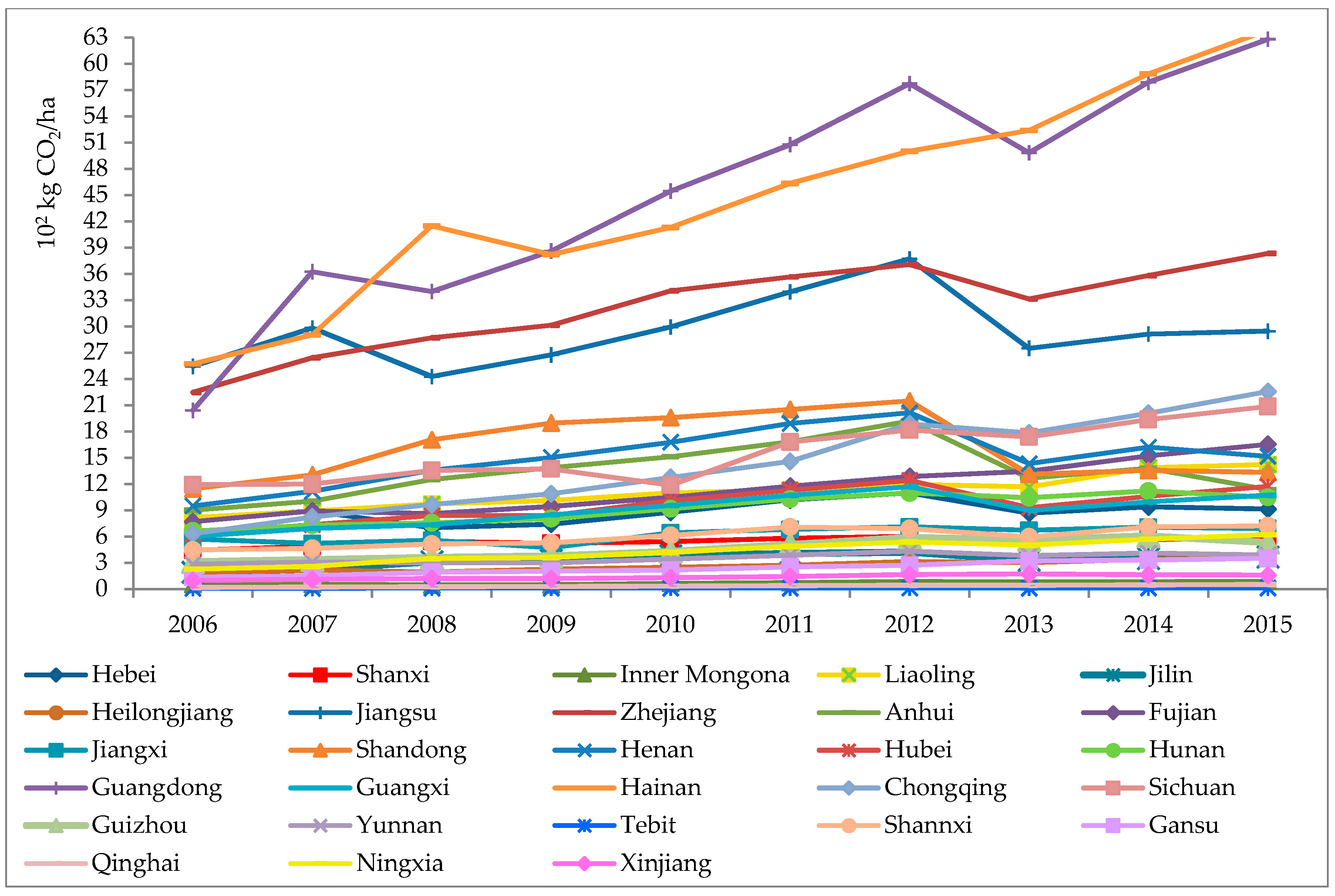
In general, the EPcfpt of all the Chinese provinces and autonomous regions increased, albeit at varying degrees, over the period 2006–2012, due to a sharp increase of passenger volumes of road, rail, and aviation transport. In 2013, the EPcfpt of many provinces and autonomous regions, except for Beijing, Tianjin, Fujian, Hainan, Gansu, and Xinjiang, showed a decline. The reasons include not only the decline of road passenger turnover, but also the decrease of specific emissions per vehicle. However, in the long run, the decrease of specific emissions per vehicle will not significantly change the total EPcfpt of China. Relatively large declines occurred in Jiangsu, Zhejiang, Anhui, Shandong, Henan and Guangdong, among which the decline of Jiangsu was the most pronounced (10.21 × 10² kg CO2/ha), i.e., a decrease above 27%. After 2013, the EPcfpt of other Chinese provinces and autonomous regions show a continuous increase.
Pressures on the productive land are very small in Inner Mongolia, Gansu, Xinjiang, Qinghai, Ningxia, which are classified as the Middle of the Yellow River and the Northwest Economic Zone, and typically have a large amount of productive land and small amounts of passenger transport. In Tibet, in particular, the EPcfpt has remained stable at a low level of 10 kg CO2/ha. The productive lands of Tibet are well protected, and the volume of passenger transport is rather low. In Hainan, rapid development of tourism in recent years has resulted in an increasing number of passengers. As a result, the EPcfpt increased to 63.84 × 10² kg CO2/ha from 25.71 × 10² kg CO2/ha in 2006, i.e., a decrease above 50%. The change of EPcfpt index for Jiangxi, Guizhou, and Shaanxi was 2.0 × 10² kg CO2/ha, which was lower than in all other provinces.
The EPcfpt values of Beijing, Shanghai, and Tianjin are very high due to rapid economic development, small amounts of productive land, and huge passenger transport turnover. The maximum EPcfpt of Shanghai is 890.25 × 10² kg CO2/ha, i.e., 89,025 kilograms of carbon emissions stored in productive land per hectare. This figure reflects the per unit productive land that absorbs the amount of carbon emissions.
According to the results of different provinces and autonomous regions in each year, it can be seen that the EPcfpt values of Beijing, Shanghai and Tianjin are outliers. The mean EPcfpt values of Beijing, Shanghai and Tianjin during the period of 2006–2015 are 341.2 × 10² kg CO2/ha, 637.8 × 10² kg CO2/ha and 66.1 × 10² kg CO2/ha, respectively, which are much higher than the mean values of the other 28 provinces and autonomous regions. In order to show the change of EPcfp of different provinces and autonomous regions more clearly, we used Figure 4 to show the change of outlier values of Beijing, Shanghai and Tianjin, and used Figure 5 to show the change of other values which basically distributed averagely. The EPcfpt values of Beijing and Tianjin showed a linear increase from 2006 to 2015 (Figure 5), and the EPcfpt values of Shanghai appeared to slightly decline in 2013, but showed a rising trend overall.
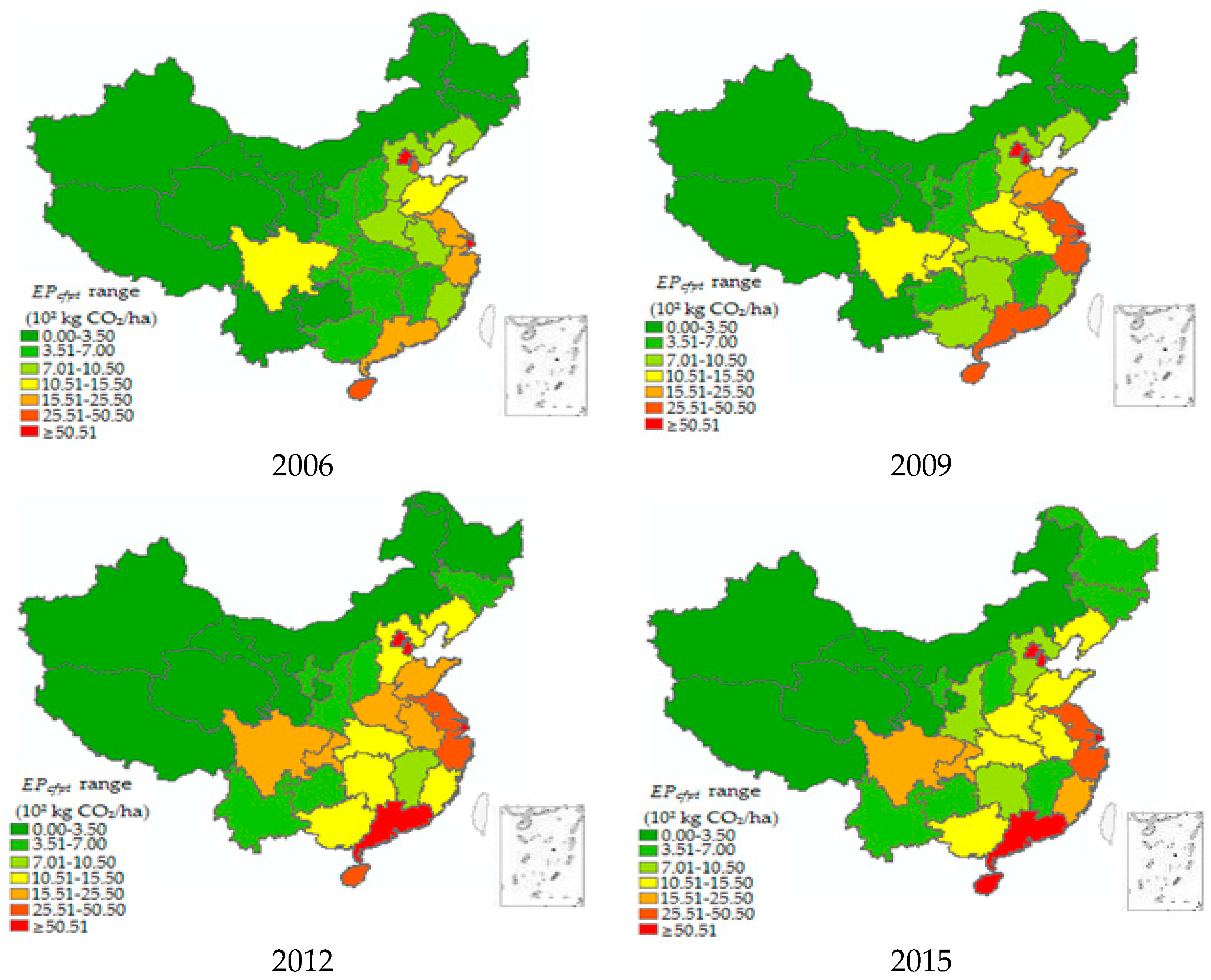
Figure 6 shows the spatial distribution of EPcfpt for all the Chinese provinces and autonomous regions in the years of 2006, 2009, 2012, and 2015. We can clearly see the spatial distribution feature and EPcfpt changes of different provinces. In general, the EPcfpt of Chinese provinces and autonomous regions have increased from different levels. The EPcfpt of Chinese eastern and central regions, especially, increased significantly. The regions with a high ecological pressure are mainly located in the eastern areas. The EPcfpt values of provinces in western areas are low.
4.2. Spatial Autocorrelation of EPcfpt in China
4.2.1. Global Spatial Autocorrelation Analysis
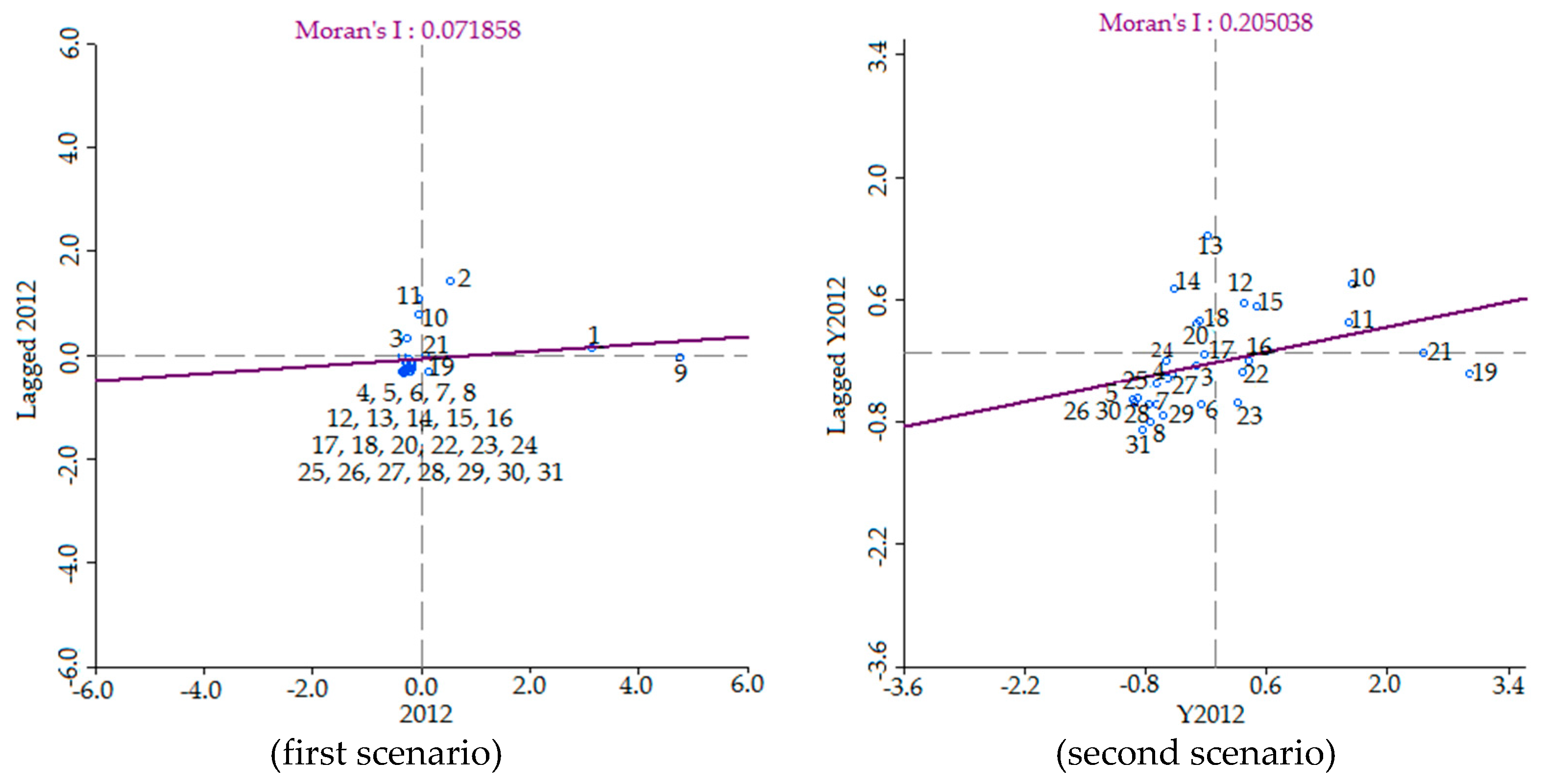
As can be seen from Table 3 and Figure 6, the outlier EPcfpt values of Beijing, Shanghai and Tianjin are very high, which might influence the global autocorrelation. Therefore, the research regions are classified into two scenarios: the first scenario is the whole province area, and the second scenario is the area without Beijing, Shanghai and Tianjin. In order to explore the effect of these outlier EPcfpt values of Beijing, Shanghai and Tianjin, we calculated Moran’s I in the two scenarios. One is to calculate Moran’s I of all China’s provinces and autonomous regions (this can be called unadjusted Moran’s I), and the other is to calculate Moran’s I of China’s provinces and autonomous regions without Beijing, Shanghai and Tianjin (this can be called adjusted Moran’s I). The results of unadjusted Moran’s I and adjusted Moran’s I are shown in the Table 4. We also chose the scatter plots of Moran’s I in the first and the second scenario in 2012, as an example, to obtain a more intuitive contrast (Figure 7).
In the first scenario (i.e., unadjusted), the results of Moran’s I index are close to 0 over the entire period of 2006–2015 (Table 4), the Z values are below 1.96 and the P values are above 0.05, so according to the standards of the spatial autocorrelation, the EPcfpt of all the provinces and autonomous regions might be randomly distributed in the province units at the 0.05 significant level. However, in the second scenario (i.e., adjusted), we found that the results of Moran’s I index are above 0 over the entire period of 2006–2015 (Table 4), which indicates that the EPcfpt of the other provinces and autonomous regions have positive autocorrelation relationships. Furthermore, this positive autocorrelation relationship was proved statistically significant because the Z values were above 1.96 and the P values were below 0.05. That is, all the EPcfpt values of the provinces and autonomous regions without Beijing, Shanghai and Tianjin showed a state of spatial aggregation. In contrast to these scenarios, we found that the outlier EPcfpt values of Beijing, Shanghai and Tianjin have great influences on the EPcfpt of the whole country. One of the most likely explanations for the results is that these regions have experienced too much passenger transport turnover compared to the amount of productive land area. From Table 4, we can find that Moran’s I-value is gradually decreasing in the second scenario, which indicates that the positive autocorrelation relationship is gradually weakening over time.
4.2.2. Local Spatial Autocorrelation Analysis
From the above analysis of the first scenario and the second scenario, we found that the special EPcfpt values of Beijing, Shanghai and Tianjin had influenced the spatial autocorrelation analysis significantly. Therefore, we removed these regions from the whole research unit area in the follow-up analysis. In this part, the local spatial autocorrelation analysis will be carried out in the provinces and autonomous regions in the second scenario.
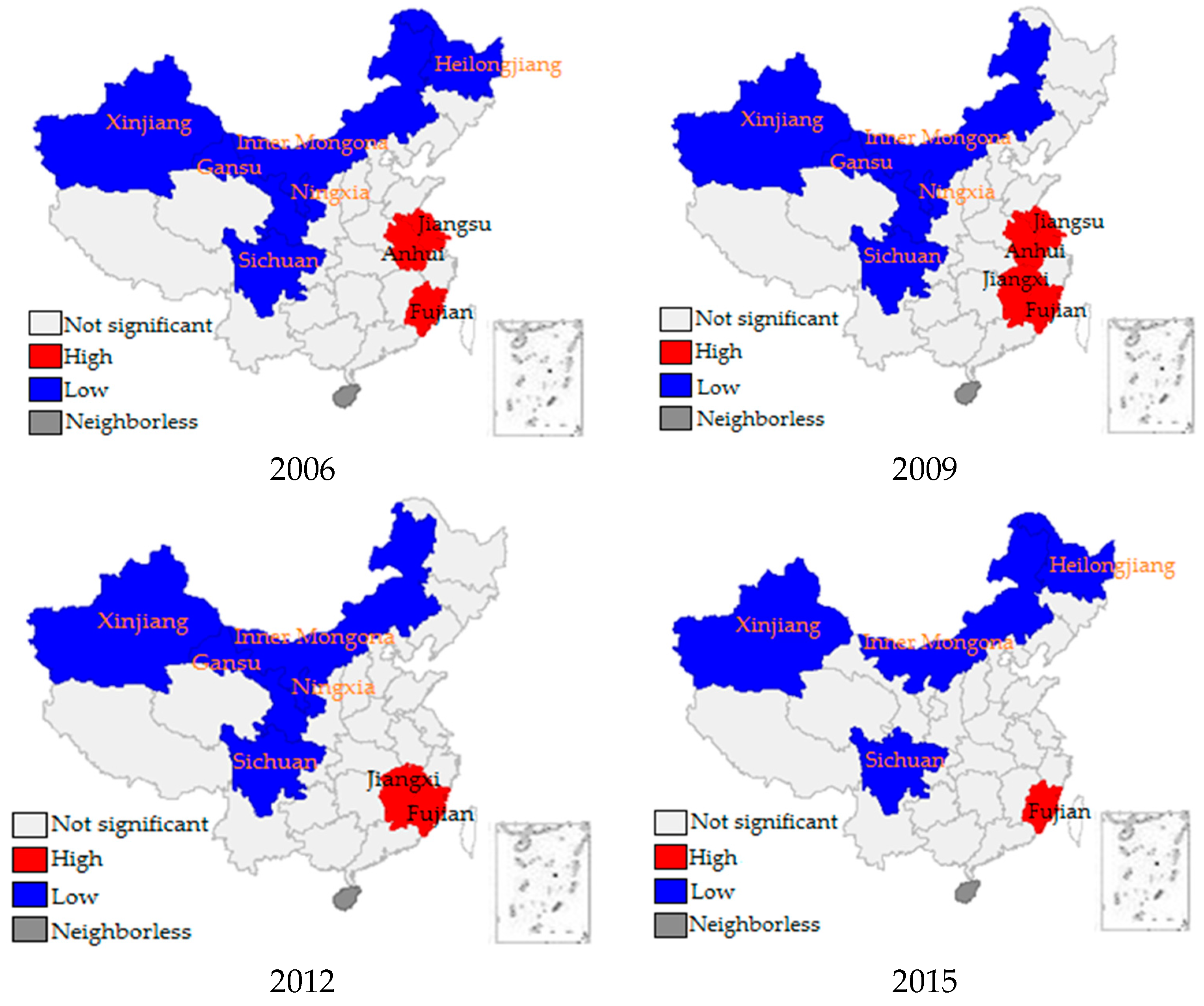
We used the local Getis and Ord Gi* to explore the local spatial autocorrelation further and distinguish the aggregation types of EPcfpt values among the other provinces. The changes of aggregation are shown in Table 5. We can see that the low aggregation provinces mainly include Xinjiang, Inner Mongolia, Heilongjiang, Gansu, Ningxia, Sichuan and Tibet, and the high aggregation provinces mainly include Jiangsu, Anhui, Fujian and Jiangxi. During the study period, there was no change concerning the low aggregation phenomenon of Xinjiang and Inner Mongolia, and the high aggregation of Fujian did not change either. The other provinces that were characterized by aggregation showed slightly different changes. Furthermore, the distribution of high and low aggregation shows obvious characteristics in terms of geography. As shown in Figure 8, the low aggregation provinces are mainly located in the northwest, while the high aggregation provinces mainly appear in the southeast of China.
4.3. Regional Disparities of EPcfpt in China’s Eight Comprehensive Economic Zones
In order to further analyze the disparities of EPcfpt values in different Economic Zones, we used the coefficient of variation from the perspective of the Eight Comprehensive Economic Zones in China. The coefficient of variation reflects the degree of data discretization and discrepancy.
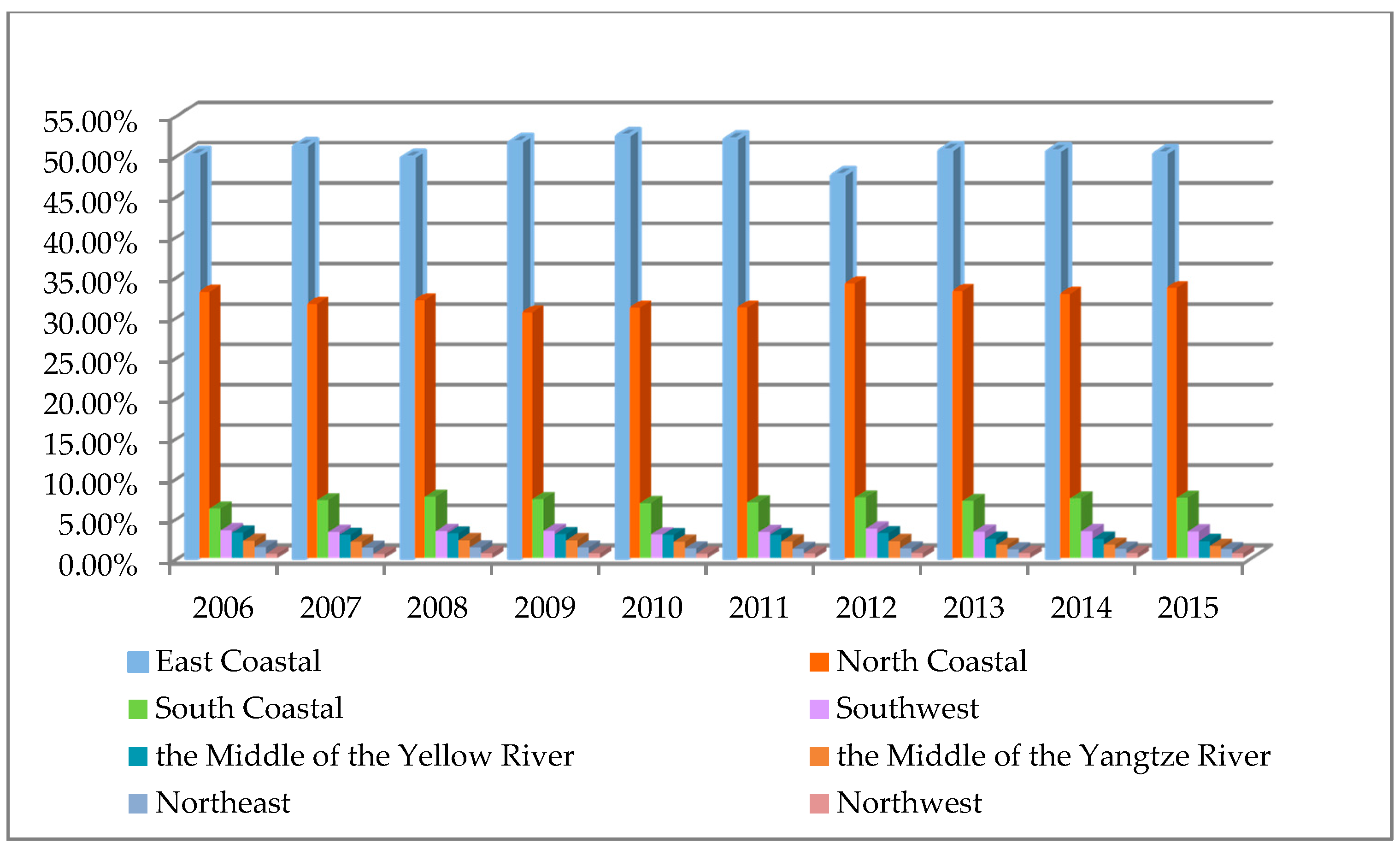
Based on the EPcfpt value of each province and autonomous region, we can obtain the total value of the EPcfpt in each Comprehensive Economic Zone. The EPcfpt values of the Eight Comprehensive Economic Zones from 2006 to 2015 are shown in Figure 9. It can be seen that the EPcfpt values in the Eastern Coastal Economic Zone are the largest and amount to about 50% of the total EPcfpt. Furthermore, the EPcfpt value of the North Coastal region is the second largest and accounts for approximately 33% of the total EPcfpt. In combination, these two Economic Zones account for more than 80% of the total EPcfpt in China.
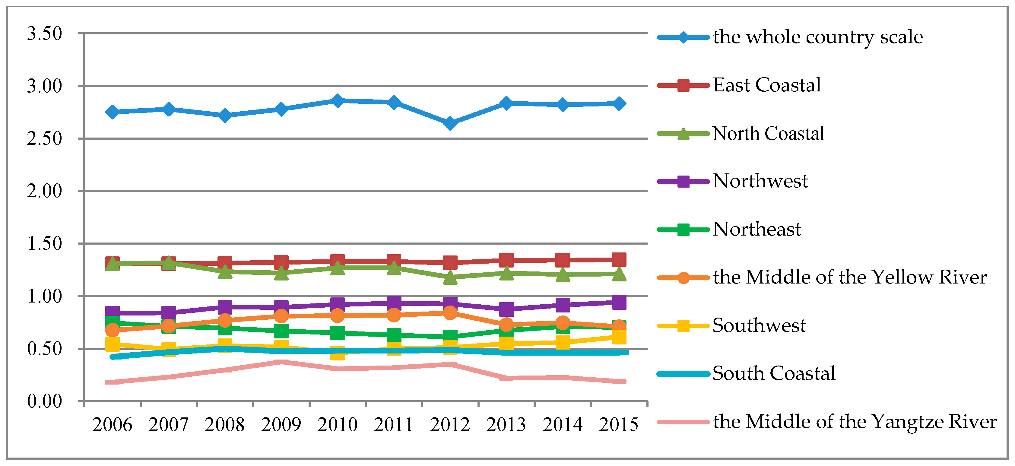
The results of the coefficient of variation (CV) for each of the Comprehensive Economic Zones and the whole country over the period 2006–2015 are shown in Figure 10. The change of CVs represents the disparity of EPcfpt values in China’s Eight Comprehensive Economic Zones and the whole country. There are three spatial trends in the EPcfpt. First, the CVs are increasing in the East Coastal, the Northwest and the Southwest Economic Zones. This means that the difference of the EPcfpt values of the provinces in these Comprehensive Economic Zones increased. Second, the CVs of the South Coastal, the Middle of the Yangtze River, the Middle of the Yellow River, and the Northeast Economic Zone have followed a fluctuating trend. Third, the CV of the North Coastal decreases by 0.1 from 2006 to 2015, which means that the regional disparity for EPcfpt is decreasing. Compared to other Comprehensive Economic Zones, the North Coastal and East Coastal Economic Zones have high variability, mainly because they include Beijing and Shanghai. The coefficient of variation of the rest of the Economic Zones is smaller, indicating that the difference in EPcfpt values of each province is smaller. However, from the perspective of the whole country, the mean CV is 2.786, which shows that the disparities of EPcfpt values for all the provinces and autonomous regions of China are very large; the main cause of this is the outlier EPcfpt values. The disparities between the different Economic Zones are closely related to their economic development, land use rate, the structure of passenger transport, and governmental policy.
5. Conclusions and Recommendations
5.1. Conclusions
Using the data from 2006 to 2015 of all the provinces and autonomous regions in China, this study presented an estimation of the ecological pressure of the carbon footprint of the passenger transport (EPcfpt). Conducting spatial analysis, we subsequently analyzed the global and local autocorrelation of EPcfpt in China’s provinces and autonomous regions. Using the EPcfpt coefficient of variation, the disparities between China’s Eight Comprehensive Economic Zones and the whole country scale were also assessed.
In general, the EPcfpt of all the Chinese provinces and autonomous regions have increased over the period of 2006–2012, followed by a reduction in 2013 due to a decrease in passenger turnover. The sharp decrease in road passenger transport turnover is mainly due to the fierce competition between road and railway transport. High-speed railways have rapidly developed since 2013. From 2013 onwards, the EPcfpt again showed a continuous increase. Provinces with large EPcfpt values were mainly concentrated in several major coastal areas, e.g., Shanghai, Beijing, and Tianjin had the highest EPcfpt, and also showed the fastest growth in the EPcfpt.
The EPcfpt of all the Chinese provinces and autonomous regions might be randomly distributed in space. However, from our analysis, the outlier EPcfpt values of Beijing, Shanghai and Tianjin are very high, which might influence the global autocorrelation. Therefore, we classified the research regions into two scenarios, and found that there are different spatial autocorrelation results in different scenarios. There are positive autocorrelation relationships in the second scenario. Furthermore, according to the local spatial autocorrelation analysis, the low aggregation provinces are mainly located in the northwest, while the high aggregation provinces appear in the southeastern of China.
The relative disparities in EPcfpt between China’s Eight Comprehensive Economic Zones varied strongly. The disparities in EPcfpt of the East Coastal, the Northwest and the Southwest Economic Zones increased over the years. The South Coastal, the Middle of the Yangtze River, the Middle of the Yellow River, and the Northeast Economic Zone followed fluctuating trends over the years. The regional disparity in the North Coastal Economic Zone decreased gradually. The EPcfpt of the North Coastal and East Coastal Economic Zone showed strong differences, because they contain Beijing and Shanghai, respectively, which are the top two regions of China in terms of EPcfpt.
5.2. Recommendations and Future Research
Rapid economic development, and the growth of passenger travel distance and frequency, will result in further increases in China’s EPcfpt. Consequently, the productive land of each province and autonomous region will be under great pressure, and the energy conservation and carbon emission mitigation will remain challenging. As such, we proposed a number of policy recommendations in relation to the reduction of EPcfpt. Foremost, based on the proposed model and the analysis results, every province or autonomous region should mitigate its passenger transport carbon emission to prevent the increasing EPcfpt. On the one hand, China should further optimize the traffic structure of passenger transport, especially in big cities such as Beijing, Shanghai, and Tianjin. For example, road transport passengers can shift to more low-carbon rail and other modes of transport. On the other hand, China should adjust the energy consumption structure of passenger transport, increase the use of natural gas, solar energy and other clean energy and reduce the proportion of petrol and diesel in passenger transport as soon as possible. Second, a stricter control policy should be created and implemented to enlarge the area of productive land, or at least inhibit further loss in order to further relieve EPcfpt. Third, based on the interaction of provinces in spatial aggregation that face more EPcfpt stress, especially the high aggregation areas such as China’s eastern regions, the government should actively carry out a collaborative policy to guide the transport sector to reduce the pressure of productive land. The low aggregation provinces should play a leading role in driving the adjacent provinces to reduce the ecological pressure of the carbon footprint of in passenger transport. Fourth, the government should vigorously advocate car sharing and guide the community to choose environmentally friendly ways to travel. This makes a profound difference in improving the efficiency of resource utilization and alleviating the ecological pressure of the carbon footprint in passenger transport in the long run.
In this study, we explored the ecological pressure of the carbon footprint in passenger transport. However, the spatial autocorrelation results of EPcfpt are subject to the modifiable areal unit problem (MAUP). The MAUP illustrates both the need for considering spatial analysis, and the fundamental uncertainties that accompany real-world analysis [49]. In the process of spatial analysis, the map of China is displayed as the geographical raster model, which is used to depict and mimic the green space of all the provinces and autonomous regions of China. However, the boundaries of space units are often created artificially or in an ad hoc manner and thus can be changed according to the data collection. Therefore, due to the limitation of data acquisition of smaller space units at present, we only analyzed the statistical results according to the spatial adjacency relationship of the province units. In a future study, we will try to collect as much data as possible on smaller units and further analyze the spatial autocorrelation in a more detailed scope.
Acknowledgments
This study was financially supported by the National Social Science Foundation of China (grant number 17BJY139), Humanities and Social Science Foundation of Ministry of Education of China (grant number 17YJCZH125); the Social Science Fund of Shaanxi Province (grant number 2016R026), and the Social Science Fund of Xi’an City (grant number 17J176).
Author Contributions
Fei Ma and Wenlin Wang conceived and established the study framework; Fei Ma developed the model and analyzed the data; Fei Ma, Wenlin Wang, Qipeng Sun, Fei Liu, and Xiaodan Li wrote the paper.
Conflicts of Interest
The authors declare no conflict of interest.
References
- Core Writing Team; Pachauri, R.K.; Meyer, L.A. Contribution of Working Groups I, II, and III to the Fifty Assessment Report of the Intergovernmental Panel on Climate Changes; Climate Change 2014: Synthesis Report; Intergovernmental Panel on Climate Changes (IPCC): Geneva, Switzerland, 2014. [Google Scholar]
- Li, Y.; Bao, L.; Li, W.X.; Deng, H.P. Inventory and Policy Reduction Potential of Greenhouse Gas and Pollutant Emissions of Road Transportation Industry in China. Sustainability 2016, 8, 1218. [Google Scholar] [CrossRef]
- Internal Energy Agency (IEA): CO2 Emission from Fuel Combustion-Highlights. Available online: http://www.iea.org/publications/freepublications/publication/name.31870.en.html (accessed on 13 April 2012).
- Dong, Q.H.; Meng, F.; Michael, Q.; Wang, K.H. Impacts of urban transportation mode split on CO2 emission in Jinan, China. Energies 2011, 4, 685–699. [Google Scholar]
- Wang, Z.J.; Chen, F.; Fujiyama, T. Carbon emission from urban passenger transportation in Beijing. Transp. Res. Part D 2015, 41, 217–227. [Google Scholar] [CrossRef]
- Mitali, D.G. Carbon Footprint from Road Transport Use in Kolkata City. Transp. Res. Part D 2014, 32, 397–410. [Google Scholar]
- Saboori, B.; Sapri, M.; Baba, M. Economic growth, energy consumption and CO2 emissions in OECD’s transport sector:A fully modified bi-directional relationship approach. Energy 2014, 66, 150–161. [Google Scholar] [CrossRef]
- Mckinnon, A.C.; Piecyk, M.I. Measurement of CO2 emissions from road freight transport: A review of UK experience. Energy Policy 2009, 37, 3733–3742. [Google Scholar] [CrossRef]
- Yin, X.; Chen, W.; Eom, J.; Clarke, L.E.; Kim, S.H.; Patel, P.L.; Yu, S. China’s transportation energy consumption and CO2 emissions from a global perspective. Energy Policy 2015, 82, 233–248. [Google Scholar] [CrossRef]
- Timilsiina, G.R.; Shrestha, A. Transportation sector CO2 emissions growth in Asia: Underlying factors and policy options. Energy Policy 2009, 37, 4523–4539. [Google Scholar] [CrossRef]
- Yang, L.; Yi, J.C.; Xiao, Z.; Yang, Q.S.; Zhi, Y.Z. A carbon emission evaluation for an integrated logistics system-a case study of the port of Shenzhen. Sustainability 2017, 9, 462. [Google Scholar] [CrossRef]
- Ercan, T.; Onat, N.C.; Tatari, O. Investigating Carbon Footprint Reduction Potential of Public Transportation in United States: A system dynamics approach. J. Clean. Prod. 2016, 133, 1260–1276. [Google Scholar] [CrossRef]
- Zheng, H.; Fang, Q.; Wang, C.; Hui, W.W.; Ren, R. China’s carbon footprint based on input-output table series: 1992–2020. Sustainability 2017, 9, 387. [Google Scholar] [CrossRef]
- Liu, H.B.; Zi, Y.; Xu, A. A comparative life-cycle energy and emission analysis for intercity passenger transportation in the U.S. aviation, intercity bus and automobile. Transp. Res. Part D 2016, 48, 267–483. [Google Scholar] [CrossRef]
- Patanavaraha, V.; Jomnonkwao, S. Trends in Thailand CO2 emissions in the transportation sector and Policy Mitigation. Transp. Policy 2015, 41, 136–146. [Google Scholar] [CrossRef]
- Seo, J.; Park, J.; Oh, Y.; Park, S. Estimation of total transport CO2 emission generation by medium-and heavy-duty vehicles in sector of Korea. Energies 2016, 9, 638. [Google Scholar] [CrossRef]
- Fan, F.Y.; Lei, Y.L. Decomposition analysis of energy-related carbon emissions from the transportation sector in Beijing. Transp. Res. Part D 2016, 42, 135–145. [Google Scholar] [CrossRef]
- Jie, F.D.; Deng, C.; Rong, R.L. Moving low-carbon transportation in Xinjiang: Evidence from STIRPAT and rigid regression models. Sustainability 2017, 9, 24–39. [Google Scholar]
- Andrade, C.E.S.D.; D’Agosto, M.D.A. The role of rail transit systems in reducing energy and carbon dioxide emission: The case of the city of Rio de Janeiro. Sustainability 2016, 8, 150. [Google Scholar] [CrossRef]
- Han, J.; Hayashi, Y. A system dynamics model of CO2 mitigation in China’s inter-city passenger transport. Transp. Res. Part D 2008, 13, 298–305. [Google Scholar] [CrossRef]
- Wiedmann, T.O.; Minx, J. A definition of ‘carbon footprint’. Ecol. Econ. Res. Trends 2008, 1, 1–11. [Google Scholar]
- Wiedmann, T.O. Carbon footprint and input-output analysis—An introduction. Econ. Syst. Res. 2009, 3, 175–186. [Google Scholar] [CrossRef]
- Melanta, S.; Miller-Hooks, E.; Avetisyan, G.H. Carbon footprint estimation tool for transportation project.Conster. Eng. Manag. 2013, 5, 547–555. [Google Scholar]
- Ribau, J.P.; Sousa, J.; Carla, M. Reducing the carbon footprint of urban bus fleets using multi-objective optimization. Energy 2015, 93, 1089–1104. [Google Scholar] [CrossRef]
- Padgett, J.P.; Steinemann, A.C.; Clarke, J.H.; Vandenbergh, M.P. A comparison of carbon calculators. Environ. Impact Assess. Rev. 2008, 28, 106–115. [Google Scholar] [CrossRef]
- Sharp, H.; Grundius, J.; Heinonen, J. Carbon footprint of inbound tourism to Iceland: A consumption-based life-cycle assessment including direct and indirect emission. Sustainability 2016, 8, 1147. [Google Scholar] [CrossRef]
- Wang, B.B.; Shao, C.F.; Ji, X. Influencing Mechanism Analysis of Holiday Activity-Travel Patterns on Transportation Energy Consumption and Emissions in China. Energies 2017, 10, 897. [Google Scholar] [CrossRef]
- Chen, G.W.; Wiedmann, T.; Wang, Y.F.; Hadjikakou, M. Transnational city carbon footprint networks—Exploring carbon links between Australian and Chinese cities. Appl. Energy 2016, 184, 1082–1092. [Google Scholar] [CrossRef]
- Xie, X.; Cai, W.J.; Jiang, Y.K. Carbon footprint and embodied carbon flows analysis for china’s eight regions:a new perspective for mitigation solutions. Sustainability 2015, 7, 10098–10114. [Google Scholar] [CrossRef]
- Zhao, R.Q.; Huang, X.J.; Liu, Y.; Zhong, T.; Ding, M.; Chuai, X. Urban Carbon Footprint and Carbon Cycle Pressure: The case study of Nanjing. J. Geogr. Sci. 2014, 24, 159–176. [Google Scholar] [CrossRef]
- Hertwich, E.G.; Peter, G.P. Carbon footprint of national: A global, trade-linked analysis. Envinon. Sci. Technol. 2009, 16, 6414–6420. [Google Scholar] [CrossRef]
- Matthews, H.S.; Hendrickson, C.; Weber, C. The importance of carbon footprint estimation boundaries. Environ. Sci. Technol. 2008, 42, 5839–5842. [Google Scholar] [CrossRef] [PubMed]
- Hillsman, E.L.; Cevallos, F.; Sando, T. Carbon footprint for public transportation agency in Florida transportation research record. J. Transp. Res. Board 2012, 10, 80–88. [Google Scholar] [CrossRef]
- Ji, X.; Chen, G.Q. Exergy analysis of energy utilization in the transportation sector in China. Energy Policy 2006, 14, 1709–1719. [Google Scholar] [CrossRef]
- Ji, X.; Chen, G.Q.; Chen, B.; Jiang, M.M. Exergy-based assessment for waste gas emissions from Chinese transportation. Energy Policy 2009, 6, 2231–2240. [Google Scholar] [CrossRef]
- Ji, X.; Chen, G.Q. Unified account of gas pollutants and greenhouse gas emissions: Chinese transportation 1978–2004. Commun. Nonlinear Sci. Numer. Simul. 2010, 19, 2710–2722. [Google Scholar] [CrossRef]
- The 13th“Five-Year” Planning about Energy Conservation and Emission Mitigation in Transportation. Available online: http://www.mot.gov.cn/zhuanti/shisanwujtysfzgh/ (accessed on 5 January 2017). (In Chinese)
- Xu, J.P.; Lin, X.Y. China’s urban passenger traffic ecological footprint calculation -to Beijing as an example. J. City Probl. 2015, 9, 74–80. [Google Scholar]
- Xu, L.H.; Wei, Y.N. An overview of carbon footprint research in transportation. J. Traffic Inf. Secur. 2014, 32, 1–7. [Google Scholar]
- Wu, P.; Shi, P.H. An estimation of energy consumption and CO2 emission in tourism sector of China. J. Geogr. Sci. 2011, 21, 744–745. [Google Scholar] [CrossRef]
- GÖsslinga, S.; Peeters, P. The eco-efficiency of tourism. Ecol. Econ. 2005, 54, 417–434. [Google Scholar] [CrossRef]
- Intergovernmental Panel on Climate Change (IPCC). Guidelines for National Greenhouse Gas Inventories; IPCC: Geneva, Switzerland, 2006; Volume 2. [Google Scholar]
- Pan, Y.D.; Birdsey, R.A.; Fang, J.Y.; Houghton, R.; Kauppi, P.K.; Kurz, W.A.; Phillips, O.L.; Shvidenko, A.; Lewis, S.L.; Canadell, J.G.; et al. A large and persistent carbon sink in the world’s forests. Science 2011, 333, 988–993. [Google Scholar] [CrossRef] [PubMed]
- He, Y.F.; Xie, H.L.; Fan, Y.H.; Wang, W.; Xie, X. Forested land use efficiency in china: Spatiotemporal patterns and influencing factors from 1999 to 2010. Sustainability 2016, 8, 772. [Google Scholar] [CrossRef]
- Zhang, S.L.; Zhang, K. Contrast study on the local indices of spatial autocorrelation. Stat. Res. 2007, 24, 65–67. [Google Scholar]
- Eight Major Economic Zones. Available online: https://baike.so.com/doc/6892804-7110349.html (accessed on 17 October 2014). (In Chinese).
- National Bureau of Statistics of the People’s Republic of China. China Statistical Yearbook; China Statistics Press: Beijing, China, 2006–2015.
- Ministry of Land and Resources of the People’s Republic of China. China’s Land and Resources Yearbook; Geological Publishing House: Beijing, China, 2006–2015.
- Openshaw, S. The Modifiable Areal Unit Problem; Geobooks; University of East Anglia: Norwich, UK, 1984. [Google Scholar]
Figure 1.
Research framework.
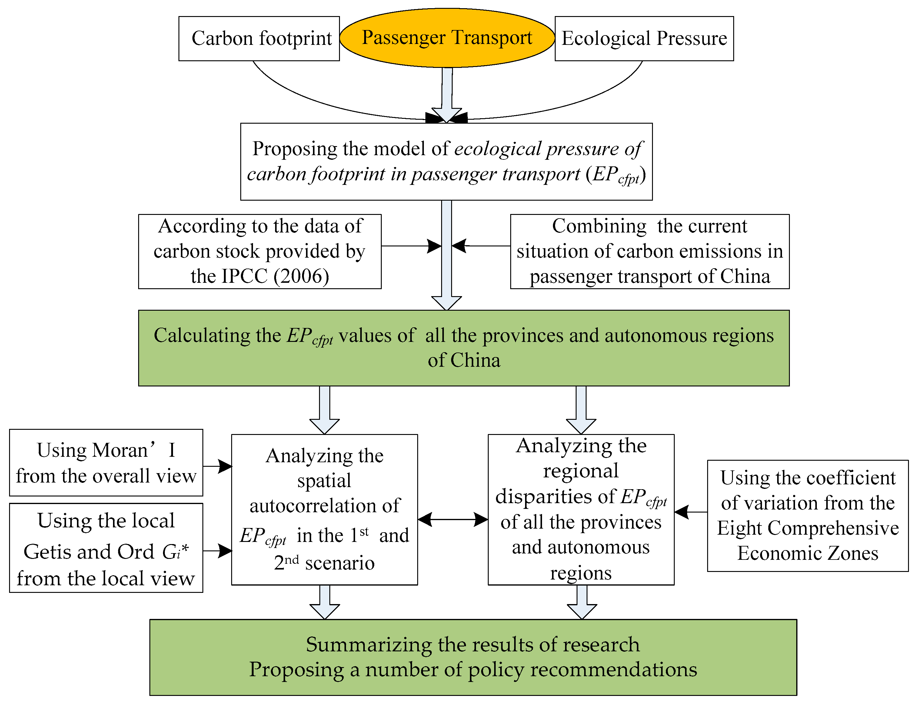
Figure 2.
The changes of passenger turnover of different transport modes from 2006 to 2015.
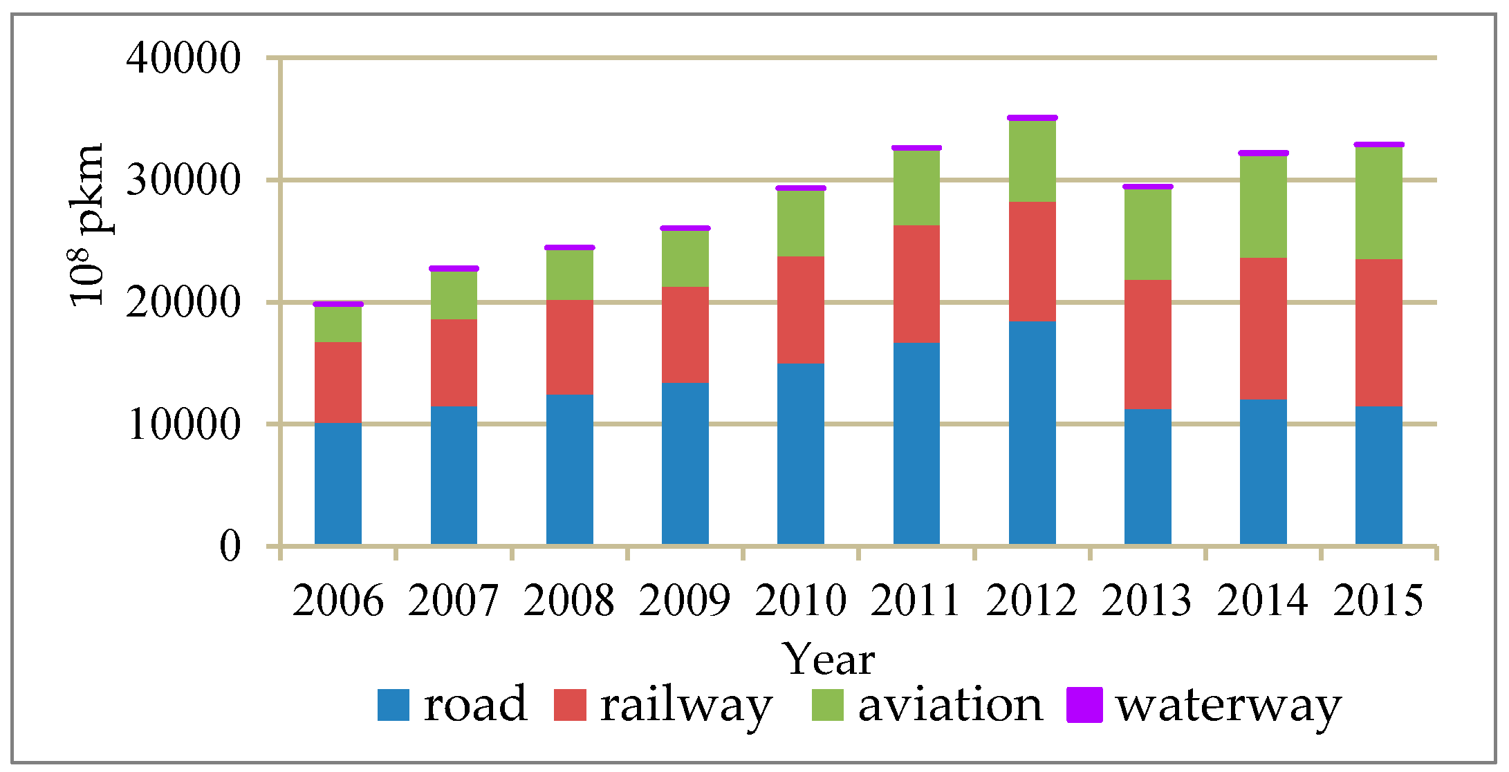
Figure 3.
The change in the productive area of the whole country.
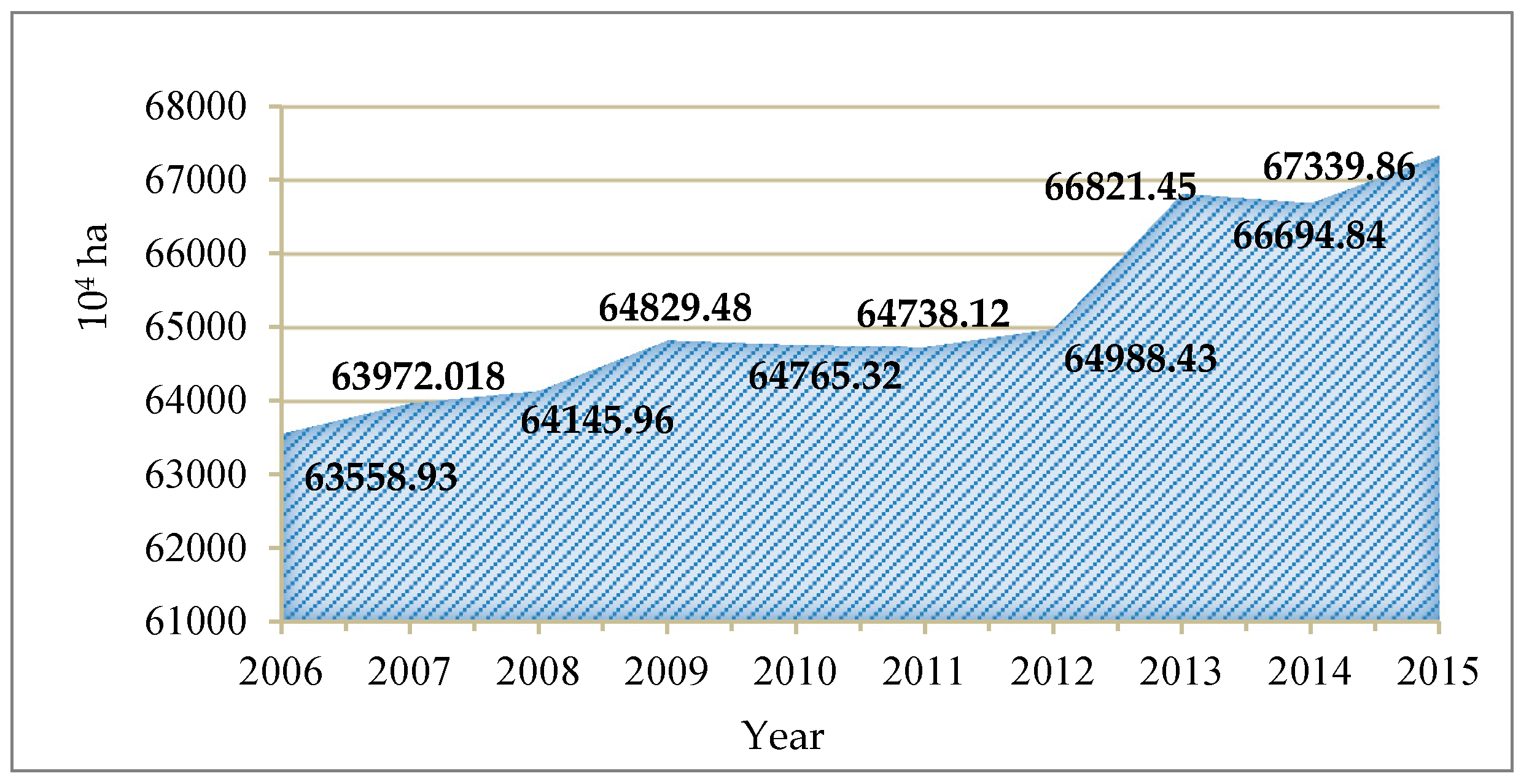
Figure 4.
The changes of outlier EPcfpt values from 2006 to 2015.

Figure 5.
The changes of other EPcfpt values from 2006 to 2015.

Figure 6.
Spatial change of EPcfpt in 2006, 2009, 2012, and 2015.

Figure 7.
The scatter plots of Moran’s I in different scenarios in 2012.

Figure 8.
The change of local space aggregation in 2006, 2009, 2012, and 2015.

Figure 9.
Proportion of EPcfpt in the Eight Comprehensive Economic Zones from 2006 to 2015.

Figure 10.
The change trend of the coefficient of variation in China.


Table 1.
Carbon emission factors of different transport modes.
| Transport Mode | Road | Railway | Aviation | Waterway |
|---|---|---|---|---|
| βi (kg CO2/pkm) | 0.132 | 0.065 | 0.369 | 0.07 |
Table 2.
The classification of the Eight Comprehensive Economic Zones.
| Economic Zones | Provinces a | Economic Zones | Provinces a |
|---|---|---|---|
| North Coastal | 1, 2, 3, 15 | East Coastal | 9, 10, 11 |
| South Coastal | 13, 19, 21 | Northwest | 26, 28, 29, 30, 31 |
| The Middle of the Yangtze River | 4, 5, 16, 27 | Southwest | 20, 22, 23, 24, 25 |
| The Middle of the Yellow River | 12, 14, 17, 18 | Northeast | 6, 7, 8 |
Note: a Province number: 1. Beijing, 2. Tianjin, 3. Hebei, 4. Shanxi, 5. Inner Mongolia, 6. Liaoning, 7. Jilin, 8. Heilongjiang, 9. Shanghai, 10. Jiangsu, 11. Zhejiang, 12. Anhui, 13. Fujian, 14. Jiangxi, 15. Shandong, 16. Henan, 17. Hubei, 18. Hunan, 19. Guangdong, 20. Guangxi, 21. Hainan, 22. Chongqing, 23. Sichuan, 24. Guizhou, 25. Yunnan, 26. Tibet, 27. Shaanxi, 28. Gansu, 29. Ningxia, 30. Qinghai, and 31. Xinjiang.
Table 3.
The EPcfpt of China’s provinces and autonomous regions from 2006 to 2015.
| Province a | Ecological Pressure of Carbon Footprint in Passenger Transport (102 kg CO2/ha) | |||||||||
|---|---|---|---|---|---|---|---|---|---|---|
| 2006 | 2007 | 2008 | 2009 | 2010 | 2011 | 2012 | 2013 | 2014 | 2015 | |
| 1 | 234.42 | 265.33 | 273.69 | 276.58 | 350.37 | 386.91 | 406.72 | 410.92 | 439.37 | 483.87 |
| 2 | 33.89 | 37.14 | 54.68 | 55.47 | 62.74 | 69.78 | 104.94 | 106.21 | 119.31 | 133.00 |
| 3 | 8.09 | 8.92 | 6.98 | 7.40 | 8.76 | 10.17 | 10.97 | 8.66 | 9.37 | 9.12 |
| 4 | 4.42 | 4.86 | 5.43 | 5.22 | 5.41 | 5.78 | 5.99 | 5.64 | 5.65 | 5.72 |
| 5 | 0.51 | 0.54 | 0.45 | 0.48 | 0.64 | 0.72 | 0.85 | 0.80 | 0.82 | 0.86 |
| 6 | 8.14 | 8.88 | 9.69 | 10.09 | 10.97 | 11.29 | 11.94 | 11.65 | 13.86 | 14.21 |
| 7 | 1.90 | 2.26 | 3.10 | 3.28 | 3.79 | 4.03 | 4.19 | 3.26 | 3.48 | 3.65 |
| 8 | 1.85 | 2.14 | 1.92 | 2.25 | 2.47 | 2.70 | 3.12 | 2.99 | 3.39 | 3.53 |
| 9 | 387.68 | 469.68 | 494.49 | 550.19 | 680.25 | 745.00 | 684.33 | 762.19 | 830.60 | 890.25 |
| 10 | 25.43 | 29.80 | 24.26 | 26.73 | 29.93 | 33.93 | 37.70 | 27.49 | 29.11 | 29.44 |
| 11 | 22.45 | 26.41 | 28.69 | 30.12 | 34.06 | 35.64 | 37.04 | 33.11 | 35.80 | 38.32 |
| 12 | 9.00 | 10.03 | 12.50 | 13.85 | 15.11 | 16.82 | 19.18 | 12.66 | 13.80 | 11.35 |
| 13 | 7.68 | 8.92 | 8.60 | 9.42 | 10.47 | 11.75 | 12.85 | 13.44 | 15.20 | 16.52 |
| 14 | 5.70 | 5.19 | 5.55 | 4.70 | 6.41 | 6.79 | 7.09 | 6.69 | 7.05 | 6.89 |
| 15 | 11.44 | 13.04 | 17.04 | 18.95 | 19.56 | 20.49 | 21.48 | 13.10 | 13.53 | 13.31 |
| 16 | 9.49 | 11.14 | 13.56 | 15.02 | 16.75 | 18.90 | 20.12 | 14.31 | 16.19 | 15.15 |
| 17 | 6.31 | 7.34 | 8.38 | 8.36 | 10.10 | 11.28 | 12.40 | 9.29 | 10.57 | 11.71 |
| 18 | 6.61 | 7.27 | 7.54 | 8.03 | 9.16 | 10.26 | 10.95 | 10.41 | 11.19 | 10.46 |
| 19 | 20.39 | 36.23 | 33.97 | 38.60 | 45.44 | 50.74 | 57.71 | 49.81 | 57.87 | 62.78 |
| 20 | 5.99 | 6.91 | 7.32 | 8.47 | 9.54 | 10.70 | 11.67 | 8.97 | 9.94 | 10.70 |
| 21 | 25.71 | 29.02 | 41.46 | 38.20 | 41.29 | 46.32 | 49.99 | 52.37 | 58.83 | 63.84 |
| 22 | 6.32 | 8.22 | 9.65 | 10.87 | 12.74 | 14.57 | 18.84 | 17.82 | 20.07 | 22.55 |
| 23 | 11.91 | 11.97 | 13.53 | 13.71 | 11.85 | 16.79 | 18.15 | 17.37 | 19.35 | 20.84 |
| 24 | 3.10 | 3.33 | 3.59 | 3.76 | 4.27 | 5.09 | 5.89 | 5.62 | 6.04 | 5.30 |
| 25 | 2.81 | 3.06 | 2.98 | 2.98 | 3.40 | 3.85 | 4.30 | 3.80 | 4.09 | 3.87 |
| 26 | 0.07 | 0.08 | 0.10 | 0.10 | 0.10 | 0.10 | 0.11 | 0.10 | 0.11 | 0.11 |
| 27 | 4.45 | 4.63 | 5.12 | 5.26 | 6.11 | 7.08 | 6.89 | 5.94 | 7.09 | 7.21 |
| 28 | 1.35 | 1.49 | 1.89 | 2.03 | 2.16 | 2.52 | 2.70 | 3.20 | 3.30 | 3.50 |
| 29 | 0.16 | 0.20 | 0.24 | 0.28 | 0.32 | 0.37 | 0.42 | 0.41 | 0.47 | 0.51 |
| 30 | 2.26 | 2.57 | 3.46 | 3.59 | 4.19 | 4.86 | 5.37 | 5.00 | 5.68 | 6.20 |
| 31 | 0.97 | 1.09 | 1.18 | 1.17 | 1.28 | 1.42 | 1.64 | 1.70 | 1.62 | 1.57 |
Note: a Province number: 1. Beijing, 2. Tianjin, 3. Hebei, 4. Shanxi, 5. Inner Mongolia, 6. Liaoning, 7. Jilin, 8. Heilongjiang, 9. Shanghai, 10. Jiangsu, 11. Zhejiang, 12. Anhui, 13. Fujian, 14. Jiangxi, 15. Shandong, 16. Henan, 17. Hubei, 18. Hunan, 19. Guangdong, 20. Guangxi, 21. Hainan, 22. Chongqing, 23. Sichuan, 24. Guizhou, 25. Yunnan, 26. Tibet, 27. Shaanxi, 28. Gansu, 29. Ningxia, 30. Qinghai, and 31. Xinjiang.
Table 4.
Global Moran’s I and related statistics under different scenarios from 2006 to 2015.
| Unadjusted (First Scenario) | Adjusted (Second Scenario) | |||||
|---|---|---|---|---|---|---|
| Year | Moran’s I-Value | Z-Value | p-Value | Moran’s I-Value | Z-Value | p-Value |
| 2006 | 0.0471 | 1.0254 | 0.135 | 0.299 | 3.093 | 0.010 |
| 2007 | 0.0423 | 0.9367 | 0.150 | 0.232 | 2.427 | 0.020 |
| 2008 | 0.0469 | 1.0349 | 0.138 | 0.204 | 2.358 | 0.018 |
| 2009 | 0.0441 | 1.0561 | 0.126 | 0.221 | 2.203 | 0.029 |
| 2010 | 0.0490 | 0.8746 | 0.116 | 0.232 | 2.465 | 0.013 |
| 2011 | 0.0541 | 0.9045 | 0.110 | 0.214 | 2.246 | 0.023 |
| 2012 | 0.0718 | 1.1480 | 0.127 | 0.205 | 2.270 | 0.025 |
| 2013 | 0.0470 | 0.9699 | 0.142 | 0.150 | 1.993 | 0.043 |
| 2014 | 0.0467 | 1.0002 | 0.146 | 0.135 | 1.978 | 0.041 |
| 2015 | 0.0478 | 1.0815 | 0.133 | 0.115 | 2.149 | 0.036 |
Table 5.
The change of low and high aggregation provinces.
| Year | Low Aggregation Provinces a | High Aggregation Provinces a |
|---|---|---|
| 2006 | 5, 8, 23, 28, 29, 31 | 10, 12, 13 |
| 2007 | 5, 8, 23, 28, 29, 31 | 12, 13, 14 |
| 2008 | 5, 23, 28, 29, 31 | 12, 13 |
| 2009 | 5, 23, 28, 29, 31 | 10, 12, 13, 14 |
| 2010 | 5, 8, 23, 28, 29, 30, 31 | 10, 12, 13, 14 |
| 2011 | 5, 23, 28, 29, 31 | 12, 13, 14 |
| 2012 | 5, 23, 28, 29, 31 | 13, 14 |
| 2013 | 5, 8, 23, 28, 29, 31 | 13 |
| 2014 | 5, 8, 23, 28, 29, 31 | 13, 14 |
| 2015 | 5, 8, 23, 31 | 13 |
Note: a Province number: 5. Inner Mongolia, 8. Heilongjiang, 10. Jiangsu, 12. Anhui, 13. Fujian, 14. Jiangxi, 23. Sichuan, 26. Tibet, 28. Gansu, 29. Ningxia, 30. Qinghai, and 31. Xinjiang.
© 2018 by the authors. Licensee MDPI, Basel, Switzerland. This article is an open access article distributed under the terms and conditions of the Creative Commons Attribution (CC BY) license (http://creativecommons.org/licenses/by/4.0/).
Share and Cite
MDPI and ACS Style
Ma, F.; Wang, W.; Sun, Q.; Liu, F.; Li, X. Ecological Pressure of Carbon Footprint in Passenger Transport: Spatio-Temporal Changes and Regional Disparities. Sustainability 2018, 10, 317. https://doi.org/10.3390/su10020317
AMA Style
Ma F, Wang W, Sun Q, Liu F, Li X. Ecological Pressure of Carbon Footprint in Passenger Transport: Spatio-Temporal Changes and Regional Disparities. Sustainability. 2018; 10(2):317. https://doi.org/10.3390/su10020317
Chicago/Turabian StyleMa, Fei, Wenlin Wang, Qipeng Sun, Fei Liu, and Xiaodan Li. 2018. "Ecological Pressure of Carbon Footprint in Passenger Transport: Spatio-Temporal Changes and Regional Disparities" Sustainability 10, no. 2: 317. https://doi.org/10.3390/su10020317
Note that from the first issue of 2016, this journal uses article numbers instead of page numbers. See further details here.