Linkage Analysis among China’s Seven Emissions Trading Scheme Pilots

Abstract

This paper focuses on the time-varying correlation among China’s seven emissions trading scheme markets. Correlation analysis shows a weak connection among these markets for the whole sample period, which spans from 9 June 2014 to 30 June 2017. The return rate series of the seven markets show the characteristics of a fat-tailed and skewed distribution, and the Vector Autoregression (VAR) residuals present a significant Autoregressive Conditional Heteroscedasticity (ARCH) effect. Therefore, we adopt Vector Autoregression Generalized ARCH model with Dynamic Conditional Correlation (VAR-DCC-GARCH) to capture the time-varying correlation coefficients. The results of the VAR-DCC-GARCH show that the conditional correlation coefficients fluctuate fiercely over time. At some points, the different markets present a significant correlation with the value of the even peaks of the coefficient at 0.8, which indicates that these markets are closely connected. However, the connection between each market does not last long. According to the actual situation of China’s regional carbon emission markets, policy factors may explain most of the temporary, significant co-movement among markets.

1. Introduction

To realize the goals of energy saving and emissions reduction policies, China’s seven ETS (emissions trading scheme) pilots were established and functioned well from 18 June 2013 to 9 June 2014. The Beijing, Tianjin, Shanghai, Guangdong, Shenzhen, Chongqing, and Hubei markets were dominated by free allocation in the pilot phase. Importantly, all seven of China’s emissions trading schemes (CETSs) were separately designed and managed. Therefore, the prices of each of the seven CETSs had their own characteristics. As is clear, these pilot schemes belong to a single country, China. From the domestic investors’ perspective, some national policies undoubtedly influence the prices of all seven CETSs. Consequently, the prices of the seven CETSs are probably connected with each other. However, the volatility of these carbon prices is inconsistent because of the specific economic structures and characteristics of carbon emissions. For example, policies about thermal power plants make the carbon prices of Hubei more volatile because Hubei province has more thermal power plants. There are all kinds of policies that affect the seven CETSs. Therefore, what are the exact co-movements among the seven CETSs? This question has attracted increasing interest from researchers examining linkages among different carbon markets, as their price movements have important implications for investment in the carbon market.

China’s carbon markets still face the problem of weak liquidity, which seriously limits the sustainable development of China’s carbon market. Therefore, it is important to conduct research on the linkage among the seven CETSs. The scales of the CETSs have been increasing in recent years, which may attract more investors. Speculators will be more concerned about the linkages between markets, and the linkage analysis may provide a reference for decision-making. Then, speculators may bring more capital into the carbon market, which may improve the liquidity and sustainability of CETSs.

In 2015, the turnover quotas of the seven national pilot carbon markets reached 37.86 million tons, and the total turnover peaked at one billion yuan. The Hubei market has the largest carbon market volume, followed by Guangdong. By the end of 2015, the quotas of the seven Chinese ETS pilots totaled 67,580,000 tons. On 27 April 2016, the first forward of carbon emissions was established in Wuhan, and the daily trading volume reached more than 680 tons with a turnover of 150 million yuan. With the establishment of a unified national carbon market, the total quotas will be four times the total annual quota of the seven pilot markets in 2014. According to the existing price and turnover rate estimations (approximately 3%), a unified national carbon market quota of spot transactions will reach four billion yuan. With the development of China’s carbon emissions markets, a growing number of investors will notice this special financial market. As for the investments in carbon emissions trading, hedging is based on linkage analysis. When trading in China’s carbon market, market managers or hedgers should not only consider the supply and demand relationship of the carbon market, but also consider whether there are linkages between the seven carbon markets. Therefore, it is very important that investors, speculators, portfolio managers, and policy makers understand the dynamic linkages among the seven CETSs.

CERs (certified emission reductions) are helpful for price co-movement from the seven carbon markets. The spreads between the EU ETS (European Union emissions trading scheme) and CERs have been explained [1], and Mansanet-Bataller [2] has shown that the spread is mainly driven by European emission allowance (EUA) prices. Moreover, Nazifi [3] has proven empirically that CERs can be considered as the primary factors underlying price spread. Barrieu and Fehr [4] used an equilibrium framework to demonstrate that compliance regulation singles out special price dynamics. Yu and Mallory [5] provided specific policy instruments generating unequal price responses that affect the spread between the two compliance instruments, such as abatement and offset usage, and delivery risks in offsets. In China, CCERs (Chinese certified emission reductions) also play an important role in carbon emission markets and may also be related to the seven CETSs. Most CCERs can be traded across regions, which means that CCERs may also act as a policy instrument promoting co-movement among the seven CETSs.

However, there seems to be little research on the dynamic linkage between carbon markets. Some studies have discussed carbon price forecasting [6,7]. For example, Zhu and Chevallier [7] adopted a hybrid ARIMA (Auto-Regressive Integrated Moving Average) model and least squares support vector machines methodology to forecast carbon prices. In addition, some research suggests that the rate of return of carbon prices was negatively associated with expected risks [8]. Zhu and Chevallier [9] studied the dynamics of only one asset, the European carbon futures price.

This paper will adopt a multi-Generalized Autoregressive Conditional Heteroscedasticity model with Dynamic Conditional Correlation (DCC-GARCH) model to investigate the dynamic linkage among emission allowance prices in China’s seven ETS pilots. The reasons are as follows. First, the rate series of return of carbon prices are high frequency time series. The DCC-GARCH model is one of the most important methods to study the dynamic correlation between two high frequency time series. Second, the carbon market presents some characteristics of financial markets. Naturally, whether the dynamic linkages among Chinese carbon markets are strengthening is a question worth considering. With the creation of carbon trading derivatives, the spot market will be more active. As is known, the DCC-GARCH model has been used to study the conditional correlation between commodities markets and financial markets, such as the oil market, gold market, exchange rate market and stock markets [10,11,12,13,14], precious metals markets, and flight-to-quality in developed markets [15]. Therefore, we may apply a multi-DCC-GARCH model to the carbon market from the financial market. Third, the DCC-GARCH model is fit for measuring dynamic correlation. The traditional Pearlman correlation coefficient no longer applies to dynamic correlation. To calculate the conditional variance, the ARCH (autoregressive conditional heteroscedasticity) model was proposed [16] and was then optimized to produce the GARCH model [17]. Afterward, in order to capture the volatility linkages among financial markets, multivariate GARCH models were proposed [18]. However, the number of parameters rises exponentially when the number of financial markets increases. To solve the parameter problem, Engle proposed the DCC (dynamic conditional correlation)-GARCH model [19]. This has been widely used in research on co-movement between financial markets, such as the research on stock market volatility spillovers [20,21], the question of the existence of financial contagion between the foreign exchange markets of several emerging and developed countries during the U.S [22], and contagion in commodity derivative markets [23,24]. Fourth, this paper studies the dynamic linkages among the seven carbon markets from an overall perspective, which requires the multi-DCC-GARCH model. When we talk about the correlation between two carbon markets, we consider the influence of the other five carbon markets on these results.

This paper makes several significant contributions to the existing literature. First, we investigate the dynamic linkages among the seven Chinese ETS pilots. At present, little research discusses this. We consider carbon markets as financial markets and convert the daily prices of the seven Chinese ETS pilots into a group of time series. Second, the DCC-GARCH model is incorporated into carbon markets for the first time to study the dynamic return transmission and volatility spillover effect. This model is generally applied in the financial markets. We adopt the method of DCC-GARCH to capture the time-varying correlation coefficients, through which we analyze the dynamic conditional correlations between the seven Chinese ETS pilots. Third, we set up a multi-DCC-GARCH model to research the dynamic correlation among the seven markets. The existing research usually builds up a bivariate DCC-GARCH model to talk about the relation between the two time series. The multi-DCC-GARCH model considers the dynamic correlation from the overall perspective.

The remainder of the paper is organized as follows: Section 2 presents the empirical model used, Section 3 presents the data and some preliminary analysis, Section 4 presents empirical findings and corresponding analysis, and finally, Section 5 concludes this paper.

2. Model

Before DCC-GARCH modeling, we calculated the correlation coefficients between every two return series. As we can see from

Table 1. Statistical analysis of daily returns of China’s seven ETS pilots.

	Mean	Median	Maximum	Minimum	sd	Skew	Kurt	JB.Test
r.sz	−0.172	0.000	22.815	−22.815	6.819	−0.150	3.561	12.347
r.bj	−0.008	0.000	37.045	−39.082	6.294	−0.601	10.904	1952.411
r.sh	−0.022	0.000	88.542	−50.425	7.122	2.255	50.953	70851.57
r.gd	−0.217	0.000	31.001	−33.647	5.860	−0.057	6.452	358.636
r.tj	−0.204	0.000	96.745	−96.745	7.909	0.345	90.126	231853.4
r.hb	−0.073	−0.037	15.616	−16.394	2.991	−0.141	8.089	793.496
r.cq	−0.412	0.000	33.564	−44.629	7.266	−1.138	10.305	1787.876

Notes: r refers to the return series of the seven markets; sz refers to Shenzhen, bj refers to Beijing, sh refers to Shanghai, gd refers to Guangdong, tj refers to Tianjin, hb refers to Hubei, and cq refers to Chongqing.

, there seem to be weak correlations between the seven ETS pilots. However, the volatility linkages between two markets cannot be explained only by the correlation coefficient, which only indicates the rough connection of a whole time period and cannot reflect the time-varying change in the linkage. To treat the changing correlations and volatilities, Engle [19] proposed the DCC-GARCH model, which has the flexibility of univariate GARCH but lacks the complexity of the conventional multivariate GARCH.

In this paper, a vector autoregression (VAR) model was fit to the series and its residuals were standardized by dividing them by their corresponding GARCH conditional standard deviation [11]. Engle described this process as “De-GARCHing” [25]. The DCC model then used these standardized residuals to estimate the dynamic conditional correlations. Our VAR-DCC-GARCH model can be depicted as follows.

For simplicity of presentation, suppose that there are two return series of carbon emission markets, $r_{1,t}$ and $r_{2,t}$, and the simple case of two series can be extended to the case of seven series.

First, the VAR model should be established. A bivariate VAR of order (p) can be expressed as follows:

$$\begin{gathered} r_{1,t}=c_1+{\alpha }_{1,1}{r}_{1,t-1}+{\beta }_{1,1}{r}_{2,t-1}+\cdots +{\alpha }_{1,p}{r}_{1,t-p}+{\beta }_{1,p}{r}_{2,t-p}+u_{1,t} \\ {r}_{2,t}=c_2+{\alpha }_{2,1}{r}_{1,t-1}+{\beta }_{2,1}{r}_{2,t-1}+\cdots +{\alpha }_{2,p}{r}_{1,t-p}+{\beta }_{2,p}{r}_{2,t-p}+u_{2,t} \end{gathered}$$

(1)

$r_{1,t}$ refers to the return of the first emissions allowance market at time t, and $r_{2,t}$ refers to the return of another market at time t. The lagged order is decided by the corresponding information criterion. After estimating the VAR (p) model, the residuals need to be collected for further DCC-GARCH modeling.

In the second step, having specified the conditional mean equation, the model was estimated conditionally according to the DCC-GARCH specification of Engle [25] to capture the volatility dynamics in the two variables. The residual $u_{i,t}$ from one of the VAR equations in Equation (1) can be represented by the following equations, in which the mean equation was also allowed to take the form of an ARMA (Auto-Regressive and Moving Average) model:

$$\begin{gathered} u_{i,t}={\theta }_0+{\epsilon }_{i,t},{\epsilon }_{i,t}~iid(0,{\sigma }_{i,t}^2) \\ {\sigma }_{i,t}^2={\alpha }_0+{{\displaystyle \sum }}_{j=1}^p{\beta }_j{\sigma }_{i,t-j}^2+{{\displaystyle \sum }}_{s=1}^q{\alpha }_s{\epsilon }_{i,t-s}^2 \end{gathered}$$

(2)

where ${\epsilon }_{i,t}$ is the standardized residual from removing the mean from the VAR residual series, which is subject to the independent identical distribution, such as a normal or t distribution. ${\sigma }_{i,t}^2$ refers to the conditional variance at time $t$, described by the GARCH (p, q) model, which can also be extended to an EGARCH (Exponential GARCH) model.

The covariance matrix in DCC-GARCH has been defined as

$$H_t=D_t{R}_t{D}_t$$

where $D_t$ is a diagonal matrix of time-varying standard deviations from the univariate GARCH models with ${\sigma }_{i,t}$.

$$D_t=\left[\begin{array}{cc}{\sigma }_{1,t}& 0\\ 0& {\sigma }_{2,t}\end{array}\right]$$

In addition, $R_t$ is the time-varying correlation matrix, where ${\rho }_{ij,t}$ is the correlation coefficient.

$$R_t=\left[\begin{array}{cc}{\rho }_{11,t}& {\rho }_{12,t}\\ {\rho }_{21,t}& {\rho }_{22,t}\end{array}\right]=\left[\begin{array}{cc}1& {\rho }_{12,t}\\ {\rho }_{21,t}& 1\end{array}\right],$$

To ensure that $R_t$ is definitely positive and that all the parameters are equal to or less than one, it can be modeled as

$$R_t=diag{\left\{Q_t\right\}}^{-1}{Q}_{t}diag{\left\{Q_t\right\}}^{-1}$$

where

$$Q_t=\left(1-{\theta }_1-{\theta }_2\right)·Q^{\ast }+{\theta }_1\left(s_{t-1}{s}_{t-1}^{’}\right)+{\theta }_2{Q}_{t-1}$$

(3)

$Q_t$ is the time-varying covariance between series, and each one of them follows a GARCH process. $s_t$ is a vector, where $s_{i,t}={\epsilon }_{i,t}/{\sigma }_{i,t}$ is further standardized by the residual ${\epsilon }_{i,t}$ with respect to the corresponding conditional standard error ${\sigma }_{i,t}$. $Q^{\ast }$ is the unconditional covariance between the series estimated in step 1. Usually, the parameters ${\theta }_1$ and ${\theta }_2$ can be estimated under the normality hypothesis of error term; however, even without the normality assumption, the estimator will still have the quasi-maximum likelihood (QML) interpretation.

3. Data Source and Statistical Analysis of Return Series

3.1. Data Source

From 18 June 2013 to 9 June 2014, China’s carbon market was in its pilot phase. During the pilot period, the main carbon market quota was distributed free of charge, and therefore, it was inappropriate to conduct research during this period. Thus, the effective sample spans from 9 June 2014 to 30 June 2017. After removing individual default data, the number of effective sample data points was 764, among which the effective trading days of 2014, 2015, 2016 and 2017 were 131, 241, 244, and 118 days, respectively.

All the daily price data of the seven Chinese ETS pilots were from the China carbon trading center website (www.tanpaifang.com).

3.2. Summary Statistical Analysis of China’s Emissions Allowance Returns

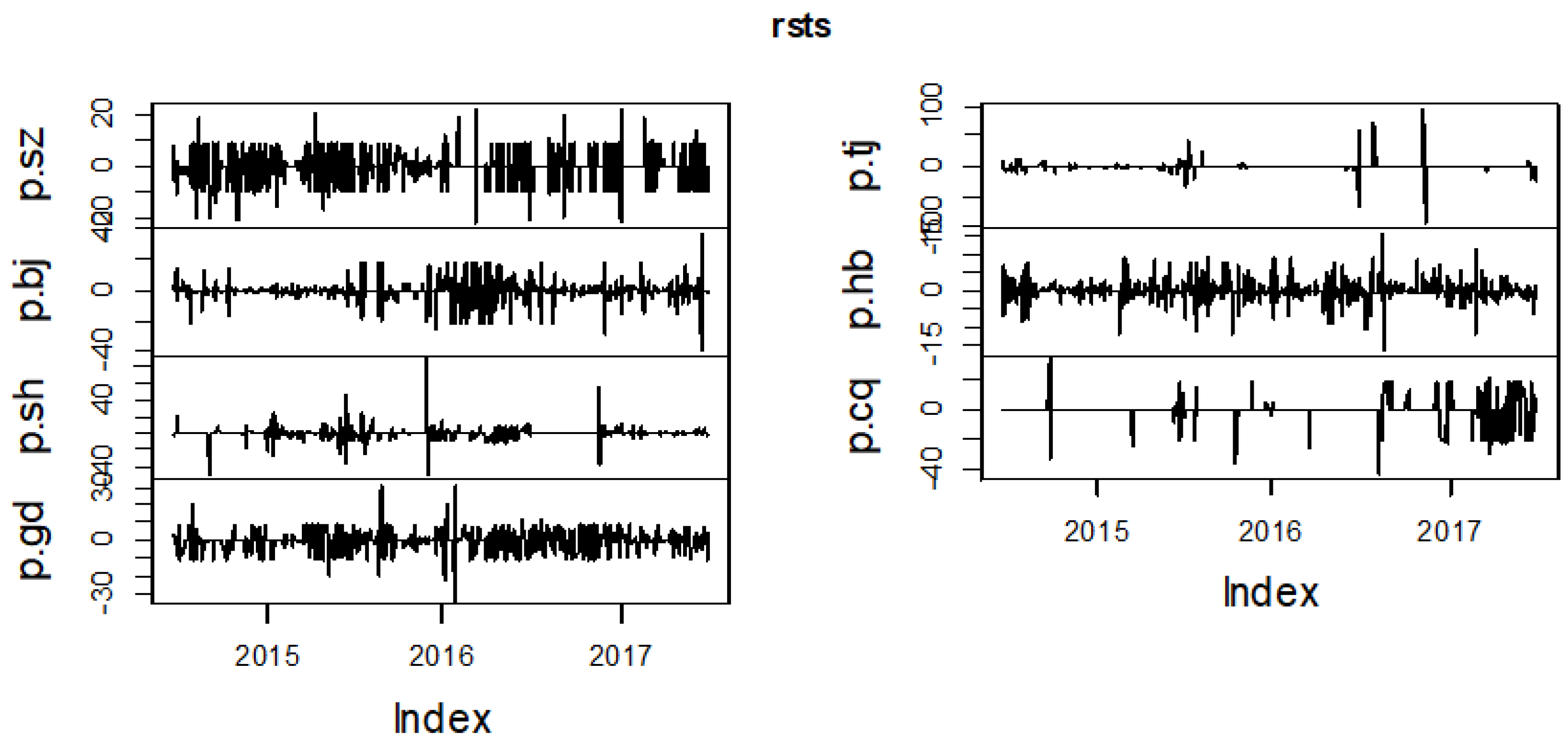
This study considered the daily closing prices for China’s seven ETS pilots to explore the co-movement between them. When we were concerned with the relevance of financial assets, we preferred to substitute the price sequence with the price returns. Hence, we defined the returns on the emissions allowances at time t as $r_{i,t}=\ln \left(\frac{p_{i,t}}{p_{i,t-1}}\right)$; $i$ denotes sz, bj, sh, gd, tj, hb, and cq. Figure 1 depicts how the returns varied over time. The returns of the Shanghai and Tianjin ETS pilots presented higher volatility than the others, and Shenzhen showed stability.

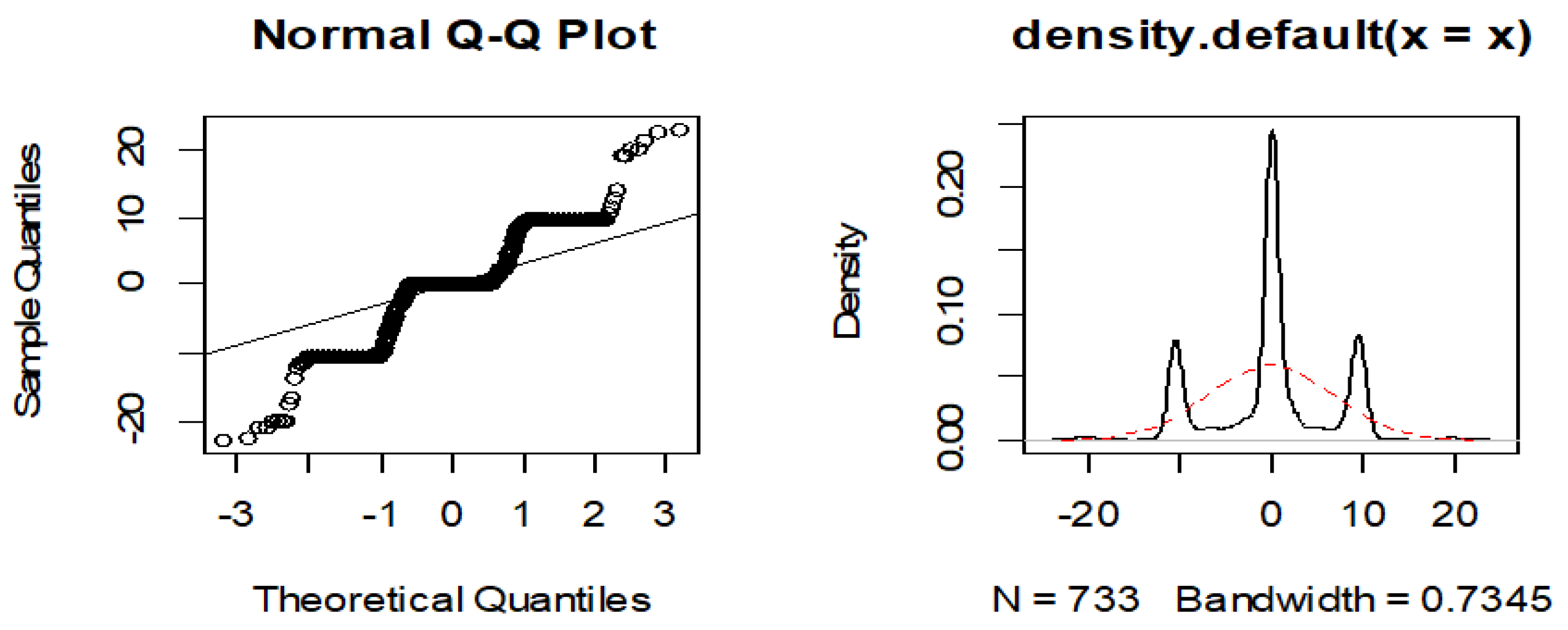
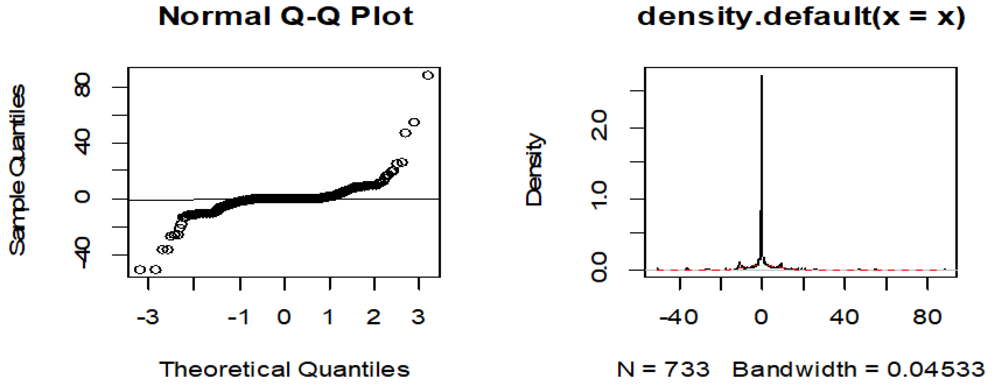
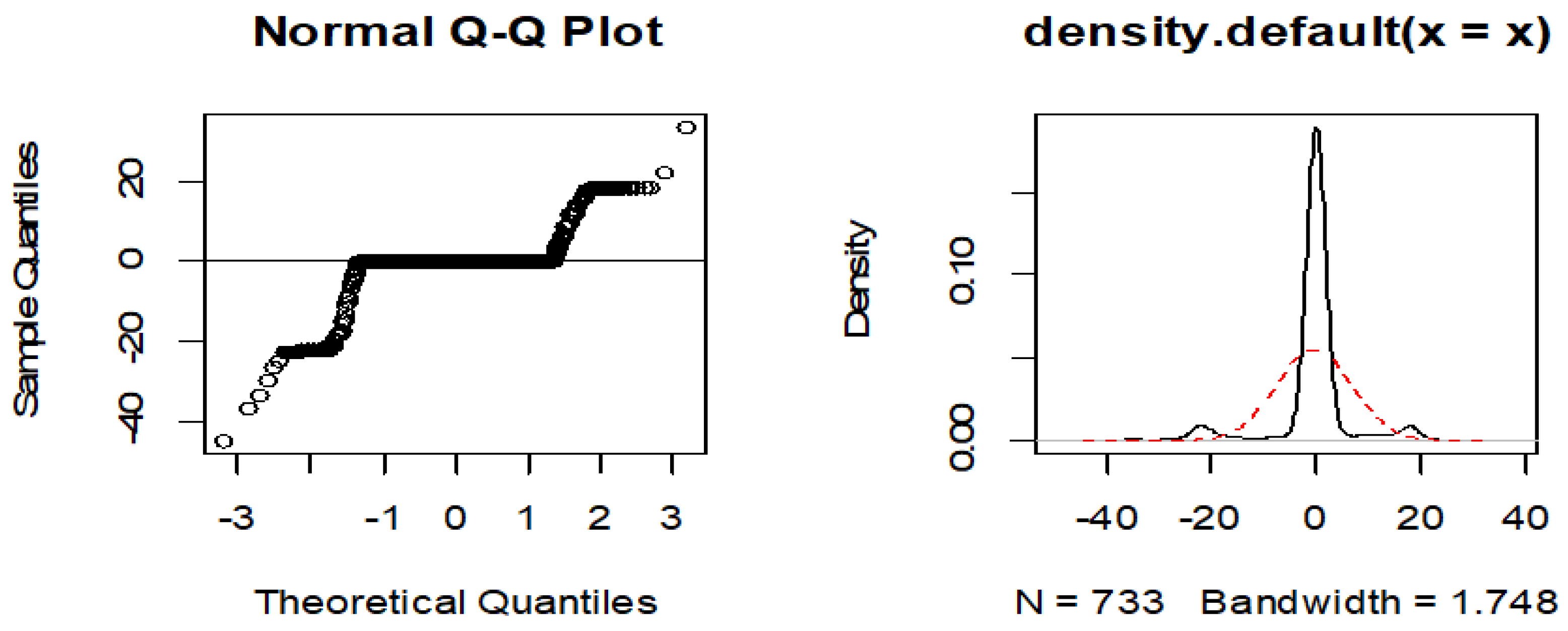
Table 1 shows the statistical analysis of the emissions allowance returns in the CETS pilots. As Table 1 shows, all emissions allowance markets presented negative returns, and the medians were almost zero, which suggests that it is not appropriate to hold an emissions allowance as a long-term asset unless under the strategy of shorting. The Tianjin emissions trading scheme market showed significant volatility, while the standard deviation of Hubei was the lowest of the CETS pilots. All the skewness values of the returns were not equal to zero, and their kurtoses were higher than three, which indicates a non-normal distribution of the returns of the seven CETS pilots. The result of the Jarque–Bera statistic confirms this conclusion. In addition, the normal quantile-quantile (Q-Q) in Figure 2, Figure 3 and Figure 4 reaffirms the judgment that the majority of the seven return series present the characteristics of a fat-tailed and skewed distribution.

4. Empirical Analysis

4.1. Correlation Analysis

Before studying the time-varying correlations, we calculated the correlation coefficients between each pair of Chinese ETS pilots, from which we could infer that the correlations between the different market prices were not strong enough. From a long-term perspective, the markets have weak interactivity with each other. In addition, from

Table 2. Correlation coefficients between the return series of China’s seven ETS pilots.

	r.sz	r.bj	r.sh	r.gd	r.tj	r.hb	r.cq
r.sz	1.0000	−0.0753	0.0045	−0.0605	−0.0098	−0.0214	0.0042
r.bj	−0.0753	1.0000	−0.0703	0.0875	0.0163	−0.0313	0.0103
r.sh	0.0045	−0.0703	1.0000	0.0399	−0.0006	0.0009	−0.0039
r.gd	−0.0605	0.0875	0.0399	1.0000	−0.0219	−0.0419	−0.0085
r.tj	−0.0098	0.0163	−0.0006	−0.0219	1.0000	0.0026	−0.0099
r.hb	−0.0214	−0.0313	0.0009	−0.0419	0.0026	1.0000	−0.0302
r.cq	0.0042	0.0103	−0.0039	−0.0085	−0.0099	−0.0302	1.0000

Notes: r refers to the return series of seven markets; sz refers to Shenzhen, bj refers to Beijing, sh refers to Shanghai, gd refers to Guangdong, tj refers to Tianjin, hb refers to Hubei, and cq refers to Chongqing.

, it can be seen that most market return series are negatively correlated. For instance, only two of the six correlation coefficients of the Shenzhen ETS pilot were positive, and all values were close to zero.

In addition, we also checked the stationarity of each return series of the emissions market through both the ADF (Automatic Direction Finder) test and the KPSS (Kwiatkowski-Phillips-Schmidt-Shin) test for unit root testing. The two kinds of checking results were similar and confirmed each other, meaning that all the series were stationary. The testing results are presented in

Table 3. Stationarity testing results.

	ADF Statistic	p-Value	KPSS Level	p-Value
r.sz	−8.9214	<1%	0.04041	>10%
r.bj	−11.404	<1%	0.02024	>10%
r.sh	−8.5035	<1%	0.42363	6.7%
r.gd	−9.7579	<1%	0.12276	>10%
r.tj	−7.4663	<1%	0.040004	>10%
r.hb	−10.762	<1%	0.08181	>10%
r.cq	−7.5633	<1%	0.1456	>10%

Notes: r refers to the return series of seven markets; sz refers to Shenzhen, bj refers to Beijing, sh refers to Shanghai, gd refers to Guangdong, tj refers to Tianjin, hb refers to Hubei, and cq refers to Chongqing.

.

4.2. Estimation of the VAR(P) Model

As mentioned in Section 2, the VAR (P) model should be estimated before DCC-GARCH modeling. Since all seven return series were stationary, we used the VAR model to formulate them.

Table 4. Empirical statistics under different information criteria.

	1	2	3	4	5
AIC(n)	25.08	25.03	25.06	25.12	25.14
HQ(n)	25.23	25.30	25.45	25.63	25.77
BICn)	25.48	25.74	26.07	26.44	26.77
FPE(n)(*1010)	7.81	7.43	7.62	8.11	8.29

presents the value of empirical statistics under different lag times according to the AIC (Akaike Information Criterion), HQ (Hannan-Quinn criterion), BIC (Bayesian Information Criterion), and FPE (Final Prediction Error) information standards. In accordance with Table 4, we obtained the optimal lag order under the AIC, HQ, BIC, and FPE information criteria. The optimum lag degrees were 2, 1, 1, and 2, respectively. Finally, we chose the results from the HQ and SC information criteria, and therefore, the optimal lag order was 1.

The result of the estimation of the VAR (1) model (vector autoregression model) is shown in

Table 5. Estimation of VAR (1) with seven variables.

	r.sz	r.bj	r.sh	r.gd	r.tj	r.hb	r.cq
r.sz(−1)	−0.1745 *** (0.000)	0.0083 (0.805)	0.016 (0.677)	−0.0051 (0.872)	−0.0443 (0.29)	−0.0094 (0.56)	−0.0604 (0.112)
r.bj(−1)	−0.0557 (0.163)	−0.2064 *** (0.000)	0.0394 (0.346)	−0.0091 (0.795)	0.0043 (0.925)	0.0068 (0.697)	−0.0105 (0.799)
r.sh(−1)	0.0188 (0.591)	−0.018 (0.575)	−0.1533 *** (0.000)	−0.0045 (0.883)	−0.02 (0.617)	0.0136 (0.378)	0.0163 (0.653)
r.gd(−1)	0.005 (0.907)	−0.0559 (0.155)	0.063 (0.161)	−0.0083 (0.823)	−0.0373 (0.445)	0.0067 (0.72)	0.0123 (0.781)
r.tj(−1)	0.0172 (0.584)	−0.0337 (0.242)	0.0252 (0.444)	0.0659 ** (0.016)	−0.2369 *** (0.000)	−0.002 (0.888)	0.0215 (0.51)
r.hb(−1)	0.065 (0.435)	−0.0127 (0.867)	0.041 (0.639)	0.0468 (0.519)	0.2397 ** (0.012)	−0.174 *** (0.000)	0.091 (0.292)
r.cq(−1)	−0.0466 (0.173)	−0.0136 (0.665)	−0.0137 (0.702)	0.0271 (0.363)	−0.0086 (0.825)	0.0073 (0.629)	0.2974 *** (0.000)
F statistic	3.928 *** (0.0003)	5.418 *** (0.0000)	3.093 *** (0.0032)	1.026 (0.4112)	7.451 *** (0.0000)	3.535 *** (0.001)	10.62 *** (0.000)

Note: r.sz refers to the return series of Shenzhen, r.sz (−1) refers to the first-order lag variable of the Shenzhen market, *** refers to the significance level of 1%, and ** refers to the significance level of 5%. The contents of the parentheses are the p-values.

, in which p.sz1 refers to the first-order lag variable, the horizontal is interpreted as the explained variable, and the column is the independent variable. There are a total of seven autoregressive equations. As is evident from Table 5, most of the equations are highly significant, except for Guangdong, which in general indicates that the first-order lag variables can explain the current prices effectively. In addition, there seems to be no linkage between the first-order lag variables and other markets, and only the first-order lag variable of the Hubei ETS has a positive feedback effect on the Tianjin price. Therefore, the lag variable has difficulty explaining the current prices of other markets, which proves that the correlations between the different price levels are not significant in the long term.

Then, we conducted the multivariate ARCH test. The value of the chi-squared statistic was 5969.1, the value of the df was 3920, and the p-value was 2.2 × 10⁻¹⁶. Obviously, we refused the null hypothesis that there was no ARCH effect.

4.3. Estimation of the VAR-DCC-GARCH Model

According to the results of the VAR (P) model with the seven variables, most of the equations were significant enough (at the 1% significance level), and the residuals of the seven equations presented a significant ARCH effect, but there was a weak linkage between the CETSs in the long run. As a consequence, we adopted the VAR-DCC-GARCH method (dynamic conditional correlation generalized autoregressive conditional heteroscedasticity), through which the dynamic conditional correlations in the short term can be measured.

In accordance with the third section, the return series of China’s ETSs present characteristics of leptokurtosis and a heavy-tailed and skewed distribution. Most of the return series show first-order autoregressive characteristics. In addition, the residuals of VAR (1) with the seven variables presented a significant ARCH effect, and this is why we employed the multivariate GARCH model. As a result of the above discussion, we considered the return series as a single variable GARCH process, where the mean equation was ARMA (1, 1), the variance equation was EGARCH (1, 1), and the residuals obeyed the skewed t distribution.

Then, we set the VAR-DCC-GARCH model of the seven variables, where the residuals followed a multivariate t distribution. In addition, we took the VAR (1) model for the mean equations to de-mean the return series and obtain the standard residuals in a VAR-DCC-GARCH framework.

Most of the parameters passed the t test. Therefore, we only took the Shenzhen market as an example, and from

Table 6. Estimation of the variance equation of the Shenzhen market.

Parameters	Estimate	Std. Error	t Value	p-Value
${\alpha }_0$	0.8408	0.1921	4.378	0.0000
${\alpha }_1$	−0.1856	0.1528	−1.215	0.2244
${\beta }_1$	0.8364	0.03139	26.64	0.0000
${\gamma }_1$	1.751	0.4313	4.060	0.0000
skew	0.9082	0.01489	60.99	0.0000
shape	2.124	0.05258	40.39	0.0000

, it is obvious that most p-values are close to zero.

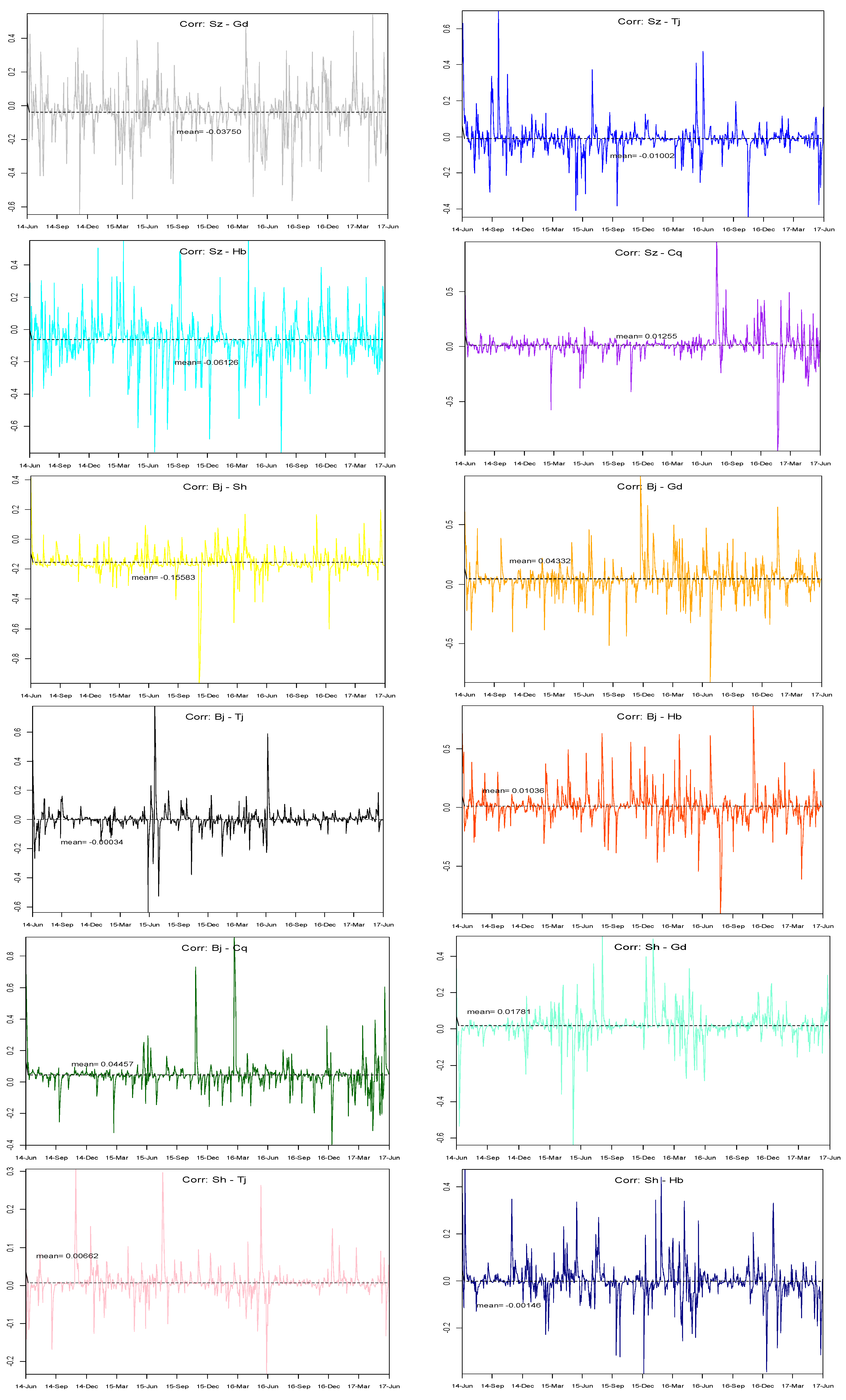
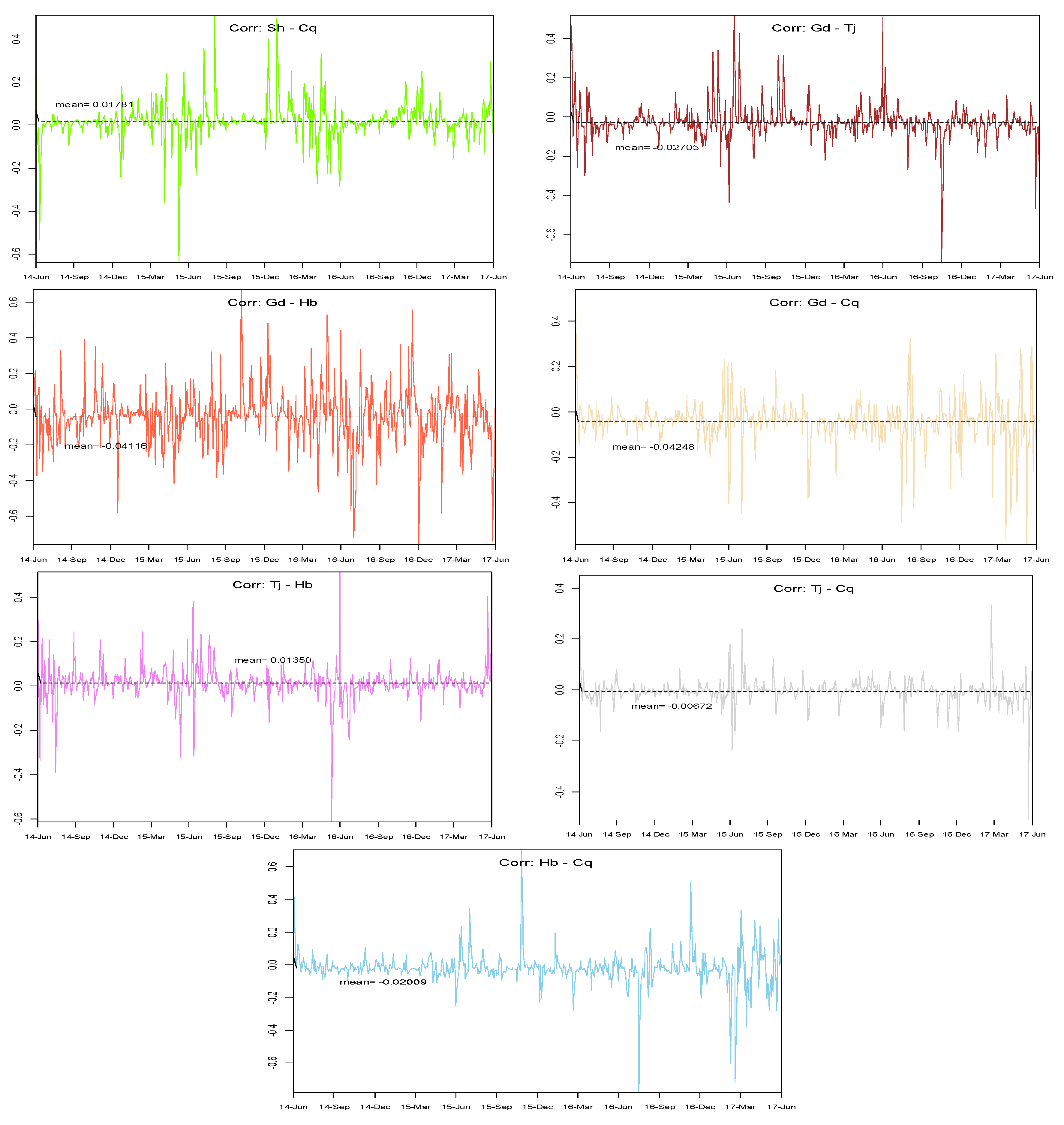
According to the results of the VAR-DCC-GARCH model, we calculated the time-varying correlation coefficients between each pair of markets and protracted the sequence diagram. As shown in the pictures, the conditional correlation coefficients were highly time variant. Despite the fact that the markets presented weak correlations over the long term, the conditional correlations may become significant at some point. Take the relationship between Beijing and Chongqing, for example. During the whole of 2015, the conditional correlation coefficient fluctuated in the range of −0.4 to 0.4, and most of the time, it was close to zero. However, at the end of 2015, the conditional correlation coefficient soared to 0.8 over an extremely short period, which indicates that the Beijing ETS was highly related to the Chongqing ETS at that point. As evidenced by the sequence diagrams of the time-varying correlation coefficients, the conditional relationships change over time and are never constant. In addition, a time interval correlation coefficient may be negative while it shifts to a positive value over time.

Although the temporary conditional correlation can rise to a high level, it is hard to find a significant linkage interval. Therefore, the co-movement between CETSs is not significant enough. As we can see from the time-varying correlation time sequence diagram, although the temporary correlations between CETSs actually appear at different points, the interval linkage was hard to find, which is in accordance with the actual situation in China. The prices of CETSs are mainly dominated by the government, and when policies change over time, the prices of different CETSs also change, which may lead to temporary linkages. However, the linkages cannot be maintained for long because the different CETSs are separately managed and regulated, and naturally, different demands will promote different price formations.

As mentioned in the introduction, different CETSs may adopt similar policies simultaneously, which explains the temporary co-movement between CETSs. For instance, at the end of 2015, the conditional correlation coefficient between Shanghai ETS and Beijing ETS reached −1.0, which can be seen in Figure 5. The high negative correlation between these two ETSs can been explained by simultaneous policies in two regions at the end of 2015. Beijing ETS changed the standards for enterprises involved in ETS at the same time. Shanghai ETS involved new sectors in the carbon markets. Moreover, in the middle of 2015, most of the CETSs (Shenzhen ETS, Shanghai ETS, Hubei ETS, and Tianjin ETS) adopted new regulations for CCER (Chinese certified emissions reduction), which simultaneously influenced the prices of carbon emissions in different CETSs. Obviously, correlation coefficients between these CETSs also deviated from the average level.

5. Conclusions

This paper focused on the time-varying correlations between China’s emissions trading scheme markets. Although there seemed to be no connection between these markets in the entire sample period, the results of VAR-DCC-GARCH show that the conditional correlation coefficients fluctuated fiercely over time, and at some points, the different markets presented significant correlations, and sometimes the coefficients even peaked at 0.8.

Up until the present moment, China’s carbon emissions markets are still dominated by the government, and naturally policies should be taken into consideration before transactions. Therefore, with regard to the reasons for temporary significant correlations between the markets of different regions, we first considered the implementation of policies. For example, when two of the seven CETS markets increase by the same quota of carbon emissions, the prices of these two markets are likely to change in synchronization, which promotes the linkage between these two regional markets. In addition, the policies of different industries may influence dynamic correlations. When the economies of two regions rely on the same high carbon industry, obviously national policies for the high carbon industry will have the same effect on the prices in their different CETSs. Therefore, for either policy makers or market participants, the results of this empirical analysis can be used as a reference for decision making. In addition, we think that cross-regional transactions may partly explain the phenomenon of high correlation, and to a certain degree, low-frequency trading activities across regions influence the formation of local market prices. Large-scale trading activities also make sense.

Although the linkages between CETSs actually appear at different points, it is hard to find a significant linkage over time. As far as we are concerned, most of the data periods are actually in the early stage of the establishment of the CETSs, and regional governments set different prices individually for the regions’ prosperity and stability. As such, it is reasonable to come to our results. Due to the fact that the information about transactions in the seven CETSs is open to the public, traders in the seven CETSs will share the same information and act similarly, and so a linkage is supposed to exist. With the development of the CETSs, more investors will enter the carbon markets, and then the prices of the CETSs will rather reflect more information about traders’ actions and expectations, after which significant linkage intervals among the CETSs will appear.

National carbon emission markets in China are expected to be established in the near future. Designing trading institutions for the national market will be a brand-new challenge for policy makers. The new national market may be selected from the seven Chinese ETSs, and thus the co-movements between the seven regional markets ought to be an essential factor worth considering. To some extent, this paper can be referred to during the establishment of the national system. For investors or market traders, the linkages between markets can be seen as an effective signal for new investment opportunities, which will attract more speculators to enter the CETSs. Then, more investments will bring more capital into the CETSs, which may improve the liquidity of the CETSs and promote the sustainable development of the CETSs.

References

- Carmona, R.; Fehr, M. The Clean Development Mechanism and Joint Price Formation for Allowances and CERs. In Seminar on Stochastic Analysis, Random Fields and Applications VI; Birkhauser: Basel, Switzerland, 2011; Volume 63, pp. 341–383. [Google Scholar]
- Mansanet-Bataller, M.; Chevallier, J.; Hervé-Mignucci, M.; Alberola, E. EUA and sCER phase II price drivers: Unveiling the reasons for the existence of the EUA–sCER spread. Energy Policy 2011, 39, 1056–1069. [Google Scholar] [CrossRef]
- Nazifi, F. Modelling the price spread between EUA and CER carbon prices. Energy Policy 2013, 56, 434–445. [Google Scholar] [CrossRef]
- Barrieu, P.; Fehr, M. Market-Consistent Modeling for Cap-and-Trade Schemes and Application to Option Pricing. INFORMS 2014, 62, 234–249. [Google Scholar] [CrossRef]
- Yu, J.; Mallory, M.L. Carbon price interaction between allocated permits and generated offsets. Oper. Res. 2017, 1–30. [Google Scholar] [CrossRef]
- Segnon, M.; Lux, T.; Gupta, R. Modeling and forecasting the volatility of carbon dioxide emission allowance prices: A review and comparison of modern volatility models. Renew. Sustain. Energy Rev. 2016, 69, 692–704. [Google Scholar] [CrossRef]
- Zhu, B.; Chevallier, J. Carbon Price Forecasting with a Hybrid ARIMA and Least Squares Support Vector Machines Methodology. Omega 2013, 41, 517–524. [Google Scholar] [CrossRef]
- Cong, R.; Lo, A.Y. Emission trading and carbon market performance in Shenzhen, China. Appl. Energy 2017, 193, 414–425. [Google Scholar] [CrossRef]
- Zhu, B.; Chevallier, J. Modelling the dynamics of European carbon futures price: A Zipf analysis. Econ. Model. 2017, 38, 372–380. [Google Scholar] [CrossRef]
- Singhal, S.; Ghosh, S. Returns and volatility linkages between international crude oil price, metal and other stock indices in India: Evidence from VAR-DCC-GARCH models. Resour. Policy 2016, 50, 276–288. [Google Scholar] [CrossRef]
- Jain, A.; Biswal, P.C. Dynamic linkages among oil price, gold price, exchange rate, and stock market in India. Resour. Policy 2016, 49, 179–185. [Google Scholar] [CrossRef]
- Caporale, G.M.; Ali, F.M.; Spagnolo, N. Oil price uncertainty and sectoral stock returns in China: A time-varying approach. China Econ. Rev. 2015, 34, 311–321. [Google Scholar] [CrossRef]
- Chkili, W. Dynamic correlations and hedging effectiveness between gold and stock markets: Evidence for BRICS countries. Res. Int. Bus. Financ. 2016, 38, 22–34. [Google Scholar] [CrossRef]
- Basher, S.A.; Sadorsky, P. Hedging emerging market stock prices with oil, gold, VIX, and bonds: A comparison between DCC, ADCC and GO-GARCH. Energy Econ. 2016, 54, 235–247. [Google Scholar] [CrossRef] [Green Version]
- Klein, T. Dynamic correlation of precious metals and flight-to-quality in developed markets. Financ. Res. Lett. 2017, 23, 283–290. [Google Scholar] [CrossRef]
- Engle, R.F. Autoregressive Conditional Heteroscedasticity with Estimates of the Variance of United Kingdom Inflation. Econometrica 1982, 50, 987–1007. [Google Scholar] [CrossRef]
- Bollerslev, T. Generalized autoregressive conditional heteroskedasticity. J. Econom. 1986, 31, 307–327. [Google Scholar] [CrossRef] [Green Version]
- Engle, R.F.; Kroner, K.F. Multivariate Simultaneous Generalized Arch. Econom. Theory 1995, 11, 122–150. [Google Scholar] [CrossRef]
- Engle, R.F. Dynamic conditional correlation: A simple class of multivariate generalized autoregressive conditional heteroskedasticity models. J. Bus. Econ. Stat. 2002, 20, 339–350. [Google Scholar] [CrossRef]
- Gamba-Santamaria, S.; Gomez-Gonzalez, J.E.; Hurtado-Guarin, J.L.; Melo-Velandia, L.F. Stock Market Volatility Spillovers: Evidence for Latin America. Financ. Res. Lett. 2016, 20, 207–216. [Google Scholar] [CrossRef]
- Mensi, W.; Hammoudeh, S.; Sang, H.K. Dynamic linkages between developed and BRICS stock markets: Portfolio risk analysis. Financ. Res. Lett. 2017, 21, 26–33. [Google Scholar] [CrossRef]
- Celık, S. The more contagion effect on emerging markets: The evidence of DCC-GARCH model. Econ. Model. 2012, 29, 1946–1959. [Google Scholar] [CrossRef]
- Roy, R.P.; Roy, S.S. Financial contagion and volatility spillover: An exploration into Indian commodity derivative market. Econ. Model. 2017, 67, 368–380. [Google Scholar] [CrossRef]
- Tsuji, C. Return transmission and asymmetric volatility spillovers between oil futures and oil equities: New DCC-MEGARCH analyses. Econ. Model. 2018, 74, 167–185. [Google Scholar] [CrossRef]
- Engle, R.F. Anticipating Correlations: A New Paradigm for Risk Management; Princeton University Press: Princeton, NJ, USA, 2009; pp. 150–152. [Google Scholar]
Figure 1.
Daily market returns of emissions allowance prices in China’s seven ETS pilots. Notes: p refers to prices of the seven markets; sz refers to Shenzhen, bj refers to Beijing, sh refers to Shanghai, gd refers to Guangdong, tj refers to Tianjin, hb refers to Hubei, and cq refers to Chongqing.
Figure 2.
Normal Q-Q (left) and kernel density (right) of the Shenzhen ETS pilot.
Figure 3.
Normal Q-Q (left) and kernel density (right) of the Shanghai ETS pilot.
Figure 4.
Normal Q-Q (left) and kernel density (right) of the Chongqing ETS pilot.
Figure 5.
Time-varying correlation coefficients between each market. Note: All the figures depict the conditional correlation coefficients between two different CETSs; Sz refers to Shenzhen, Bj refers to Beijing, Sh refers to Shanghai, Gd refers to Guangdong, Tj refers to Tianjin, Hb refers to Hubei, and Cq refers to Chongqing.