Estimating Forest Carbon Fluxes Using Machine Learning Techniques Based on Eddy Covariance Measurements


1
Key Laboratory of Coalbed Methane Resources and Reservoir Formation Process of Ministry of Education, China University of Mining and Technology, Xuzhou 221116, China
2
School of Resources and Geosciences, China University of Mining and Technology, Xuzhou 221116, China
*
Author to whom correspondence should be addressed.
Sustainability 2018, 10(1), 203; https://doi.org/10.3390/su10010203
Submission received: 30 October 2017
/
Revised: 8 January 2018
/
Accepted: 10 January 2018
/
Published: 17 January 2018
(This article belongs to the Special Issue Forests as a Key Climate Solution)
Abstract
:Approximating the complex nonlinear relationships that dominate the exchange of carbon dioxide fluxes between the biosphere and atmosphere is fundamentally important for addressing the issue of climate change. The progress of machine learning techniques has offered a number of useful tools for the scientific community aiming to gain new insights into the temporal and spatial variation of different carbon fluxes in terrestrial ecosystems. In this study, adaptive neuro-fuzzy inference system (ANFIS) and generalized regression neural network (GRNN) models were developed to predict the daily carbon fluxes in three boreal forest ecosystems based on eddy covariance (EC) measurements. Moreover, a comparison was made between the modeled values derived from these models and those of traditional artificial neural network (ANN) and support vector machine (SVM) models. These models were also compared with multiple linear regression (MLR). Several statistical indicators, including coefficient of determination (R2), Nash-Sutcliffe efficiency (NSE), bias error (Bias) and root mean square error (RMSE) were utilized to evaluate the performance of the applied models. The results showed that the developed machine learning models were able to account for the most variance in the carbon fluxes at both daily and hourly time scales in the three stands and they consistently and substantially outperformed the MLR model for both daily and hourly carbon flux estimates. It was demonstrated that the ANFIS and ANN models provided similar estimates in the testing period with an approximate value of R2 = 0.93, NSE = 0.91, Bias = 0.11 g C m−2 day−1 and RMSE = 1.04 g C m−2 day−1 for daily gross primary productivity, 0.94, 0.82, 0.24 g C m−2 day−1 and 0.72 g C m−2 day−1 for daily ecosystem respiration, and 0.79, 0.75, 0.14 g C m−2 day−1 and 0.89 g C m−2 day−1 for daily net ecosystem exchange, and slightly outperformed the GRNN and SVM models. In practical terms, however, the newly developed models (ANFIS and GRNN) are more robust and flexible, and have less parameters needed for selection and optimization in comparison with traditional ANN and SVM models. Consequently, they can be used as valuable tools to estimate forest carbon fluxes and fill the missing carbon flux data during the long-term EC measurements.
1. Introduction
Forest ecosystems play a critical role in sequestering atmospheric carbon dioxide [1,2]. The magnitude of carbon sequestration in different forest stands at various timescales ranging from hour to inter-annual is seriously influenced by global environmental change, such as climate, land use, CO2 enrichment, nitrogen deposition and biotic invasions. In addition, the substantial impacts of climate extreme events (e.g., droughts, precipitation, wind storms, heat waves, frosts and fires) on the terrestrial carbon cycle have been revealed by a few recent studies [3,4]. These effects may alter the growth patterns of pine species and biodiversity as well as the structure and functioning of forest ecosystems [5,6], which will lead to a major impediment in our understanding of the underlying mechanisms causing the ongoing seasonal variation in carbon fluxes, mainly including gross primary production (GPP), ecosystem respiration (R) and net ecosystem exchange (NEE). Therefore, quantification of the carbon exchanges between the forest ecosystems and the atmosphere is challenging for current modeling techniques, due to the complex interactions and feedbacks involved in biological, physical and chemical processes across various spatial and temporal scales.
Mechanism-based land surface models have been extensively used for estimating the terrestrial carbon fluxes from site to regional scales. However, the modeling ability of land surface models is limited because of lacking the flexibility and robustness to capture the nonlinear characteristics. Moreover, to a large extent, the fixed parameters within the models pose a challenge for the interpolation and extrapolation of the well-established models, maybe owing to the inherent variability of model parameters at various temporal and spatial scales. Therefore, considering the constantly varying statistical features in natural ecosystems, mechanism-free models were strongly recommended by Schindler and Hilborn [7] and Ye et al. [8], as a useful paradigm to handle the nonlinear interactions of non-equilibrium dynamical and complex ecological systems. Inspired by this as well as the recent availability of a great deal of data obtained by the eddy covariance (EC) technique from three different flux towers, we here used the mechanism-free machine learning techniques to simulate and predict the carbon fluxes of terrestrial forest ecosystems.
Over the past two decades, machine learning techniques have been growingly utilized to deal with the different issues involved in carbon flux estimates [9,10,11,12,13], such as filling the missing data of carbon fluxes and climatic driving factors based on the flux tower measurements [14,15], reducing the predictive errors of carbon fluxes from the land surface models [16,17] and upscaling the carbon fluxes of terrestrial ecosystems from site to regional scale on the basis of multi-source remote sensing data [18,19]. In particular, several lines of evidence have demonstrated that machine learning techniques, mainly including two traditional artificial neural network (ANN) and support vector machine (SVM) methods, have sufficiently strong ability to elucidate the nonlinear relationship between ecosystem-based carbon fluxes and environment variables based on EC measurements [13,20]. For example, Melesse and Hanley [21] utilized the ANN approach to estimate the carbon flux in three different ecosystems (grassland, cropland and forest) using the air temperature, soil temperature and several energy fluxes as input data and found that ANN could be successfully applied in simulating the ecosystem-based carbon fluxes. Dou et al. [22] used the ANN method to map different carbon and water fluxes in three Douglas-fir Stands in the Pacific Northwest based on long-term measurements and found that the use of ANN could be effective to determine the responses of three different carbon fluxes (GPP, R and NEE), evapotranspiration and water use efficiency to nitrogen fertilization. Evrendilek [23] compared the three different data-driven methods, including multiple linear regression, ANN and SVM, to estimate the influences of both atmospheric and hydrological drivers on monthly NEE using three years of measurements at a peatland site in northwestern Turkey and obtained satisfactory predictive accuracy.
On the other hand, in recent years, another two advanced machine learning modeling techniques, namely adaptive neuro-fuzzy inference system (ANFIS) and generalized regression neural network (GRNN), have been successfully applied in other fields, such as estimation of reference evapotranspiration [24,25], evaporation prediction [26,27], stream-flow forecasting [28,29], and groundwater level prediction [30,31]. These two methods have been widely acknowledged, to a large extent, due to their capability and efficiency in solving complicated nonlinear problems with only a few variables. Moreover, ANFIS method is designed through integrating fuzzy inference rules into adaptive neural networks with the intention of extracting useful knowledge involved in the trained networks in the form of fuzzy logic expression [32] and thus can conquer the weakness of knowledge interpretation for neural networks. Unlike both ANN and SVM approaches, GRNN method has the advantage of quick speed of learning, because it does not need a large number of iterations to determine optimal inner algorithms or parameters [33]. To the best of the authors’ knowledge, no research has been undertaken to date that applies both the GRNN and ANFIS approaches to predict the carbon fluxes at the ecosystem level using the EC-based data.
The present study attempts to model and predict the carbon fluxes based on the continuous six-year EC measurements in three old-growth forests under different climates. The major goal of this research is to investigate the feasibility of GRNN and ANFIS in terms of estimating the carbon flux exchanges between the biosphere and the atmosphere. Further, the results of both the well-established GRNN and ANFIS models are compared with those of commonly used ANN and SVM models and traditional empirical model (multiple linear regression, MLR). The secondary objective of the study is to examine the modeling differences among the three primary components of carbon exchanges, including gross primary production (GPP), ecosystem respiration (R) and net ecosystem exchange (NEE).
2. Materials and Methods
2.1. Site Description and Data Used
Measurements of carbon fluxes were conducted at three sites in Canada. The three sites were chosen for this study because they represent different types of forests and have obvious differences in stand age and biological structure. In addition, continuous multi-year half-hourly measurements of CO2 flux with EC technique were collected from these sites. The two forest sites, CA-Oas and CA-Obs, are situated near the southern boundary of the boreal plain ecological region in north-central Saskatchewan, Canada. The two sites were established based on the dominant boreal tree species. The two forest sites have the similar characteristics of synoptic meteorological forcing, while present the remarkable differences in their soil texture, topography and tree stem density. CA-Oas site is located in Prince Albert National Park, Saskatchewan, Canada. This mature trembling aspen site is s a boreal deciduous broadleaf forest generated from a fire in 1919, and had a mean canopy height of 22 m and an average stand age of 75 years in 2004 [34]. CA-Obs site is located about 80 km east-northeast of CA-Oas, and is predominately covered by black spruce with an average canopy height of 7.2 m. According to the statistics from the nearest long-term weather station during 1971 to 2000, the mean annual air temperature and cumulative annual precipitation are 0.4 °C and 467 mm, respectively, for both CA-Oas and CA-Obs sites [34]. CA-Gro site is situated about 80 km southwest of Timmins in northeastern Ontario, Canada. The site is a representative of the boreal mixed wood forest and was regenerated after the high level logging which primarily occurred in the 1930s. This site is primarily covered by five different types of species, including black spruce, balsam fir, trembling aspen, white spruce and white birch. At the CA-Gro site, the mean annual air temperature and cumulative annual precipitation during the study period (2004–2006, 2008–2010) are 3.29 °C and 784 mm, respectively. More details on the sites are presented in Table 1.
Based on the EC technique, continuous half-hourly carbon fluxes for six or more years were measured at each site. Positive NEE stands for a loss of CO2 to the atmosphere, while negative NEE implies an uptake of CO2 by the ecosystem. The method of gap-filling for eddy covariance-measured NEE and its partitioning into GPP and R was according to the Fluxnet-Canada Research Network protocol [38]. Briefly, R was obtained from both nighttime and cold-season NEE. The gap-filling of missing R during nighttime and calculation of R during daytime were on the basis of an empirical relationship between R and soil temperature. Finally, GPP was estimated based on the daytime-observed NEE and calculated daytime R. During the cold season, GPP was set to zero. More details regarding the EC instrument characteristics, NEE gap-filling and its separation scheme as well as the random errors in NEE, R and GPP have been provided for CA-Oas and CA-Obs in Griffis et al. [35] and Zha et al. [34], and CA-Gro in McCaughey et al. [37].
Meteorological variables were also observed, mainly including air temperature (Ta), net radiation (Rn), relative humidity (Rh), wind speed, volumetric soil moisture content and soil temperature (Ts). The EC measurements began in April 1996, May 1999, and July 2003 at CA-Oas, CA-Obs, and CA-Gro, respectively. Table 2 presents the daily statistical parameters of the used data during a period of six years. At the three sites, the correlation values for both GPP and R are generally greater than those for NEE. The variables, Ta, Ts and Rn, show strong positive correlation with both GPP and R, while have negative correlation with NEE.
2.2. Machine Learning Methods
2.2.1. Artificial Neural Network
The ANN model with a parallel computing system is widely recognized owing to its strong ability of approximating the non-linear relationship between inputs and outputs. ANN approach is widely recognized as an important supervised technique for addressing various issues, such as regression and classification, in a wide range of fields [39,40,41]. Commonly, the feed-forward neural network is the most classic ANN model and was used here in the present study. This network structure includes three different types of layers, namely, input layer, hidden (intermediate) layer and output layer. The present work used only one hidden layer because even for a specific ANN model with a single hidden layer, it can also approximate any continuous multivariate function with reasonable precision. The optimal number of hidden units selected for a specific network with lowest error during the validation period is determined through varying the number of hidden neurons on the basis of the corresponding data set. For the purpose of determining the optimum weights and thresholds of multilayer neural networks, the back propagation algorithm was adopted in this study with the aim to minimize the error between the actually simulated and expected targets from outputs for each case. Moreover, Levenberg-Marquardt algorithm was used as the training function by this study, because of its superiority of faster learning speed over some traditional conjugate gradient algorithms.
2.2.2. Support Vector Machine
The SVM model has rapidly gained popularity over the past few decades, since it was first proposed by Vapnik [42]. This advanced machine learning technique is essentially focused on addressing the classification and regression problems, which are involved in a broad range of research fields. A noteworthy innovation of SVM method is that, when solving the estimated error between the measured and the calculated, SVM depends on the structural risk minimization principle, which was introduced by Vapnik [42] in order to obtain an optimum network structure through minimizing the so-termed penalized empirical risk. This principle seeks to constrict the upper boundary on the desired risk and has some distinct superiority over conventional empirical risk minimization algorithm, which is adopted by the traditional neural network techniques. Just owing to this noticeable difference, several lines of evidence support that the SVM method presents a more powerful generalization ability than many neural network methods. When developing a SVM model, selecting a proper kernel function is of particular importance. To ensure the predictive accuracy, several kernel functions, including polynomial, sigmoid, radial basis functions, were compared and evaluated based on our applied data sets. Many attempts were made by this study and the radial basis function (RBF), which achieved the best performance, was utilized for all the SVM models. In addition, three critical parameters, including kernel width of RBF, the value of cost function and insensitive loss coefficient, were together optimized according to the grid search procedure.
2.2.3. Adaptive Neuro-Fuzzy Inference System
The ANFIS method is considered to be a sophisticated machine learning technique, and was introduced by Jang [32], based on the aforementioned ANN and fuzzy inference system (FIS). ANFIS is a more interpretable model and can offer more robust results than traditional ANN method, primarily due to the fact that it is able to qualitatively and quantitatively elucidate the nonlinear relationship between inputs and outputs through utilizing systematically the respective strengths of both ANN and FIS techniques. When developing a specific ANFIS for a given training data set, selecting a proper FIS is a major task. There are two widely used types of FISs, namely, Sugeno system [43] and Mamdani system [44]. The former was adopted by this study due to the implicitly of design in the consequent part and high computational efficiency. For a specific ANFIS model, there are generally two types of parameters that need to be optimized, the premise parameters and the consequent parameters. In the present study, the hybrid learning algorithm are composed of gradient descent algorithm and least-squares method, which were used to optimize the premise parameters and the consequent parameters, respectively. Generating a FIS is an important issue, which can be performed using several methods, such as grid partitioning, mountain and subtractive clustering. The grid partitioning algorithm is widely utilized, but the use of this method is substantially impeded owing to the curse of dimensionality. For this reason, the subtractive clustering technique was adopted by this study. Detailed description of subtractive clustering algorithm can be found in Cobaner [45].
2.2.4. General Regression Neural Network
GRNN as a feed-forward neural network could be usually subsumed under the category of radial basis function network. It is proposed by Specht [33] based on nonlinear regression theory and hence can be used as an alternative machine learning technique for approximating any arbitrary function of input-output variables from a given training dataset. In comparison with the conventional ANN approach based on back propagation algorithm, the major strengths of GRNN method can be summarized in the following aspects: (1) the simplicity of the network structure that heavily depends upon the number of input and output variables as well as the sample size of a specific training dataset, and does not necessitate any modification during the learning process; (2) the quick speed of learning as the GRNN does not require to be trained by using an time-consuming iterative procedure which must be carried out for ANN according to the back propagation algorithm with a huge amount of computation; (3) the solution of the problem of local minimum through the use of Gaussian radial basis kernel function as the transfer function in the pattern layer. In addition to these strengths, another noteworthy point is that the GRNN model does not need many iterations to determine its inner algorithms or parameters, except for the spread factor that may substantial influence the model generalization capability. In this study, the optimal spread factor selected from a set of alternative ones in the range of 0.01 to 1 was determined by using an iterative algorithm with fourfold cross-validation. More details about the GRNN method can be found in Specht [33] and Kisi [46].
2.3. Model Implement and Evaluation
In this study, four different machine learning methods, ANN, GRNN, ANFIS and SVM, were investigated and compared to estimate daily carbon fluxes in three forest ecosystems. In addition, the MLR model was also used in this investigation with the intention of examining the strength of machine learning approaches against traditional regression technique. The correlation coefficient values between environmental variables and each carbon flux in all the ecosystems have been given in Table 2. The results showed that all the carbon fluxes were highly correlated with Ta, Ts and Rn, implying that these variables were the most effective parameter influencing carbon fluxes. To obtain an accurate and reasonable comparison of modeling performance among different carbon fluxes, the applied methods with different variable combinations for inputs were tried in this study. For the sake of convenience, these abbreviated models are summarized in Table 3. We used all the models for each flux in order to make the comparison of various carbon fluxes as fair as possible.
Complete 6-year environmental and carbon flux data were used at all the sites. These data were divided into three datasets. The first 4-year dataset was used for training, the fifth year dataset was used for validation for the purpose of avoiding over-fitting and assuring the ability of model generalization, and the last 1-year dataset was for testing. It is noteworthy that all the applied models were separately trained and extrapolated for validation and prediction, owing to the differences in age among the three sites. Before the training of the applied models was started, all input and output variables were normalized between 0 and 1, respectively. The computer programs of all the machine learning models and statistical analysis of estimated results were undertaken in MATLAB (version 8.2, The Mathworks, Inc., Natick, MA, USA). Coefficient of determination (R2), Nash-Sutcliffe efficiency (NSE), bias error (Bias) and root mean square error (RMSE) were considered for the performance evaluation of the used models. These performances indices are defined as below:
where and denote the observed and modeled values of daily carbon fluxes, respectively; and are the means of observed and modeled values, respectively; is the number of observed values.
3. Results
3.1. Modeling of Daily Gross Primary Productivity
The performance indices, including R2, NSE, Bias and RMSE, are used to evaluate the accuracy of the employed models in predicting the daily GPP, R and NEE in three different forest stands in the present study. Table 4 shows the estimated accuracy of the applied models in the prediction of daily GPP in the testing period at the three sites. It is clearly seen from Table 4 that the models with full environmental variables (Ta, Rn, Rh, Ts) have the best accuracy for each method and site. Therefore, the following comparisons of the used models are mainly based on the inputs using these four variables. The developed machine learning models are consistently superior to the corresponding MLR models at the three sites. Regarding the comparisons of the machine learning models at CA-Obs site, the ANN model is superior to the other models in the testing period. However, the GRNN model generally provides the worst performance. The overall model efficiency of the used models can be ranked as follows: ANN, ANFIS, SVM, GRNN and MLR according to the R2, NSE, Bias and RMSE metrics. Similar to CA-Obs site, the GRNN model also gives the worst performance among the four machine learning models in the testing period at CA-Oas site, while the ANFIS model generates the best estimates. The overall ranks of the used models in the testing period can be summarized as follows: ANFIS, SVM, ANN, GRNN and MLR. Unlike CA-Oas site, the ANN model in the testing period performs the best at CA-Gro site. Additionally, the ANFIS and SVM models have the similar model efficiency and they are both slightly superior to the GRNN model.
In order to examine the efficiency of each model in predicting the GPP, R and NEE in all the three stands, the overall mean accuracy of each model for all the stands in the testing period is provided in Table 5. It is apparent from the table that the MLR model in the prediction of GPP generally has the worst accuracy in the testing period, whereas the ANN, ANFIS and SVM models yield the similar performance with the higher values of R2 ranging from 0.922 to 0.927 and NSE from 0.901 to 0.909. Furthermore, to provide deeper insight into the responses of different forest stands to the applied models in the prediction of daily GPP, R and NEE, the mean performance of all machine learning models for each site in the testing period is summarized in Table 6. As demonstrated in the table for GPP prediction, the models yield the best precision at CA-Obs site, and give similar results at both CA-Oas and CA-Gro sites.
Figure 1 and Figure 2 illustrate the comparisons of daily GPP between observed and predicted using the data-driven models at the three sites in the form of scatter plot and time series graph, respectively. As clearly seen from Figure 1, the fit lines of the models (ANN, GRNN, ANFIS and SVM) during the testing period for CA-Oas site appear to be consistent with the ideal fit lines (), whereas at CA-Obs site, these models have higher values of R2 and NSE than those of the corresponding models for CA-Oas and CA-Gro stands (Table 4 and Table 6). Moreover, all the five models generate more scattered estimates at both CA-Oas and CA-Gro sites in comparison with CA-Obs site.
On the other hand, as demonstrated in Figure 2, the over- and under-estimation of the best model for each site in predicting daily GPP among the training, validation and testing periods are examined. It is apparent from Figure 2 that most of the simulated values from the best ANN model in the testing period (the last 1 year) are substantially underestimated at CA-Obs site, while greatly overestimated at CA-Gro site. This is also confirmed by the aforementioned scatter plots in Figure 1.
3.2. Modeling of Daily Ecosystem Respiration
The estimated precision of the used models for predicting daily R in the testing period in the three sites are provided in Table 7. As shown from the table, the models with full input variables (Ta, Rn, Rh, Ts) perform the best for each method and site. The machine learning models with these variables consistently outperform the corresponding MLR models at both CA-Obs and CA-Oas sites, but at CA-Gro site, all the five models provide similar estimates. Specifically at CA-Obs site, the ANN model performs the best among the four machine learning models in the testing period, with respect to R2, NSE and RMSE. The predictive precision of the ANFIS is similar to that of the SVM. These two models give the inferior performance. As a whole, the GRNN model provides the lowest precision in the prediction of daily R. At CA-Oas site, the GRNN model is also inferior to the other three models (ANN, ANFIS and SVM) in terms of R2, NSE and RMSE. Besides, the ANFIS model performs the best among the five models. In conclusion, the overall model rankings of the applied models over the testing period can be ranked as follows: ANFIS, ANN, SVM, GRNN and MLR. In contrast to CA-Obs and CA-Oas sites as mentioned before, the GRNN model yields the best performance among the five models at CA-Gro site according to the four performance indices. In addition, the ANFIS performs the second best. The ANN and SVM models give similar accuracy.
On the other hand, it is clearly seen from Table 5 that the GRNN model in the three stands for forecasting daily R gives the best accuracy in the testing period, in terms of NSE, Bias and RMSE. However, the MLR model gives the worst accuracy. The ANN, ANFIS and SVM models achieve similar performance, according to the four indices. As shown in Table 6, no apparent performance indicator is found among the three stands in the prediction of daily R using the five data-driven models. Nevertheless, it should be noted that at CA-Gro site, the models give the best accuracy in terms of R2 and NSE indices.
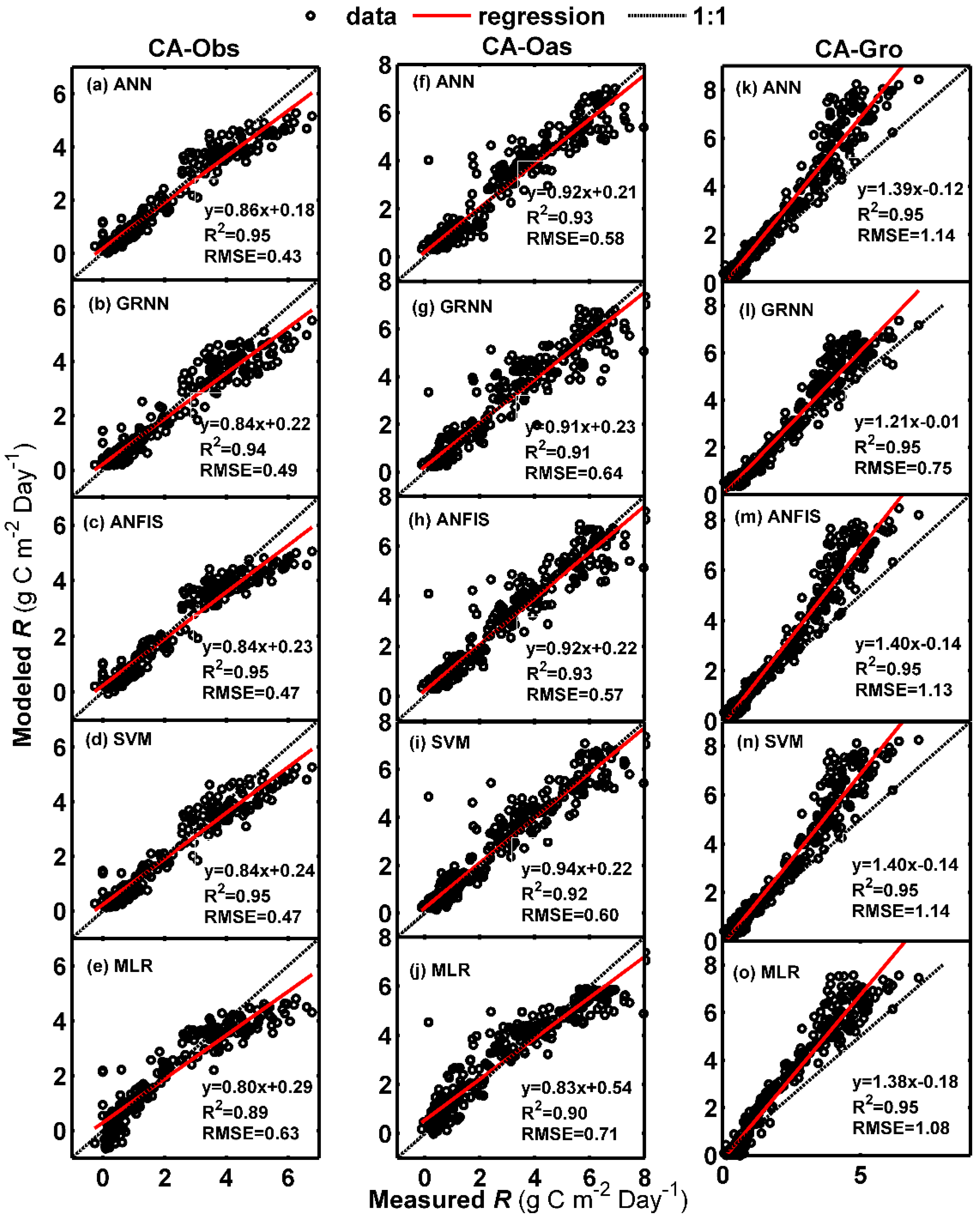
Figure 3 presents the comparisons of daily R between observed and predicted using the five models at the three sites in the form of scatter plot. As shown in Figure 3, although the regression fit lines between measured and estimated R by the ANN, GRNN, ANFIS and SVM models at CA-Oas stand are closer to the 1:1 lines, higher mean values of R2 = 0.937 and NSE = 0.925 are obtained by the models at CA-Obs site (Table 6). Besides, these models at CA-Obs site display less scattered estimates than those at CA-Oas and CA-Gro sites.
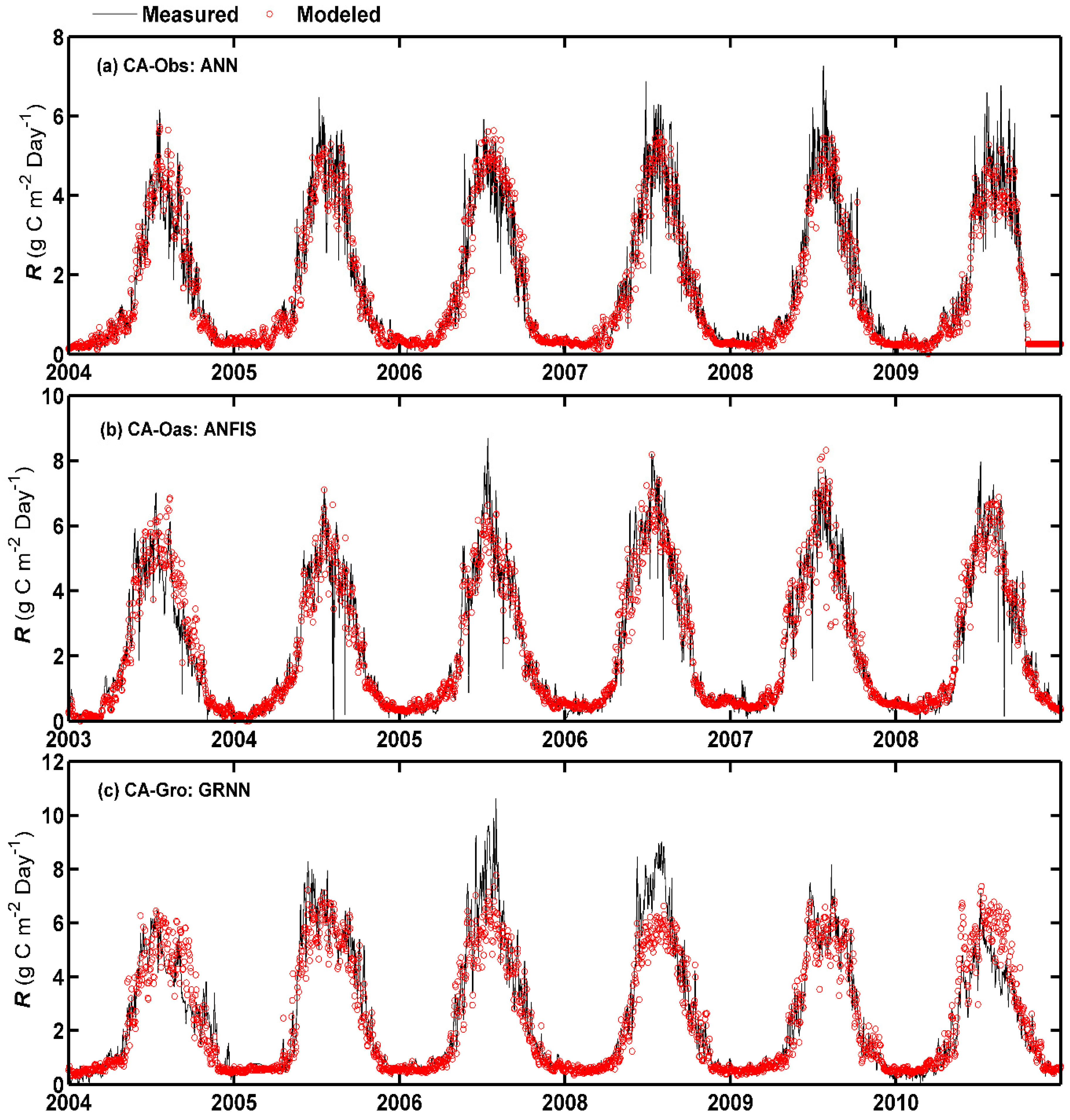
It is evident from Figure 4 that the distribution of predicted values versus observed values for daily R in the testing period varies among different sites. Similar to the time series comparison of daily GPP in Figure 2, the under- and over-estimation of the best model (especially in the peaks) in forecasting daily R in the testing period are clearly seen at CA-Obs and CA-Gro sites, respectively, as shown in Figure 4. This is consistent with the scatter plots in Figure 3 as mentioned before.
3.3. Modeling of Daily Net Ecosystem Exchange
Table 8 summarizes the accuracy of the applied models for forecasting daily NEE in the testing period. It can be clearly seen from the table that the models with full input variables (Ta, Rn, Rh, Ts) generate the best accuracy for each method and site. The four machine learning models with these variables consistently perform better than the corresponding MLR models at the three sites. At CA-Obs site, the ANN model generally gives the best precision among the five models. The SVM, GRNN and ANFIS models yield similar accuracy in terms of R2, NSE and RMSE. Unlike CA-Obs site, the ANFIS model at CA-Oas site is superior to the other models in terms of R2, NSE and RMSE. In addition, the ANN and SVM models have similar accuracy in predicting the daily NEE and they both outperform the GRNN model. At CA-Gro site, the modeling performance among the ANN, GRNN and ANFIS models is nearly consistent in the testing period. These three models are superior to the SVM and MLR models. As shown in Table 5, regarding the prediction of daily NEE, the ANN, ANFIS and SVM models achieve similar mean accuracy for the three sites. However, the MLR model gives the worst accuracy. Furthermore, it can be seen from Table 6 that the models for daily NEE prediction provide similar performance for CA-Obs and CA-Oas sites according to R2 and NSE criteria. Generally, the applied models for these two sites perform better than those for CA-Gro site.
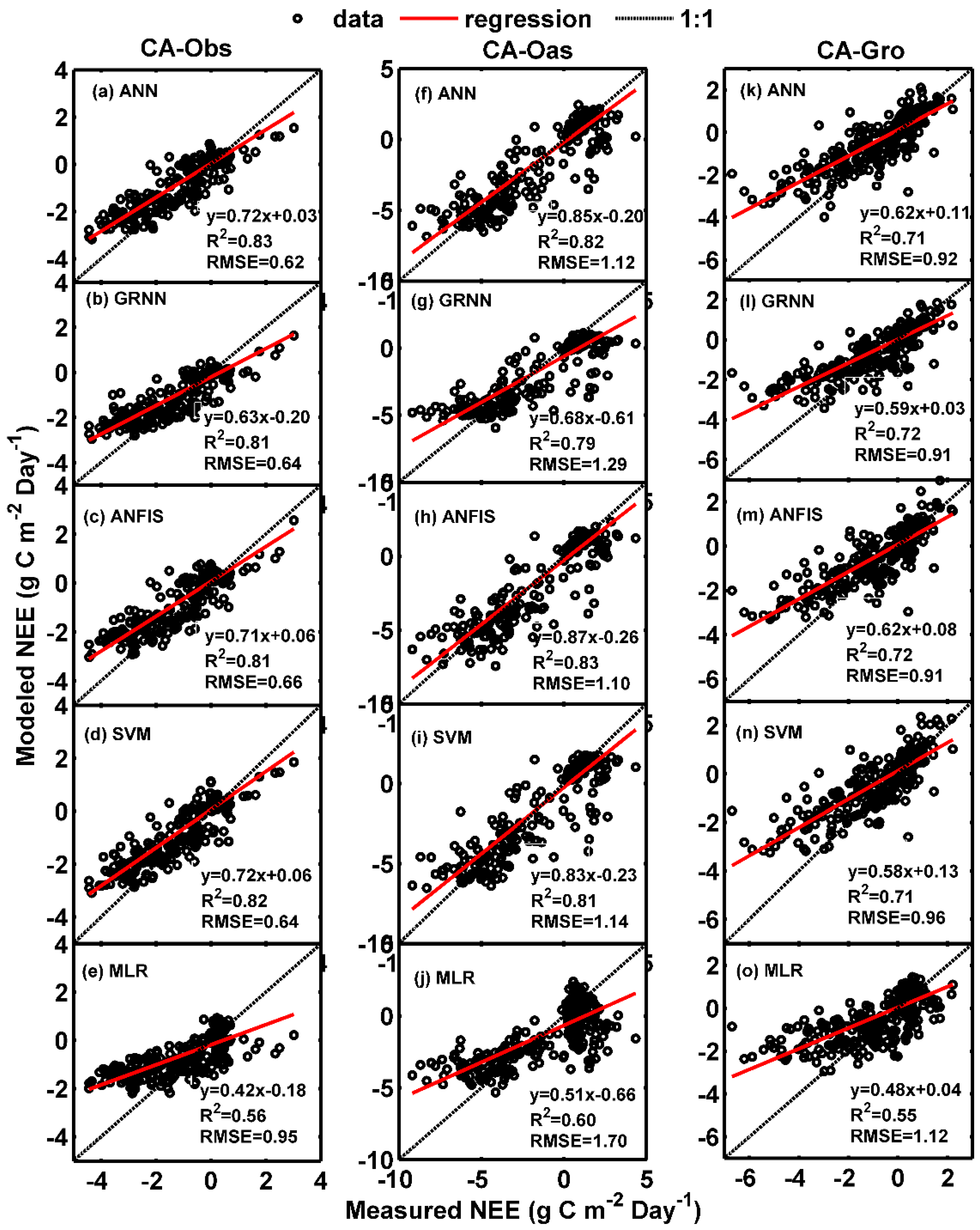
The measured and predicted values of daily NEE using the five models for the three stands are compared in Figure 5 and Figure 6. It is apparent from Figure 5 that the fit lines of the applied models during the testing period at CA-Obs and CA-Oas sites are closer to the ideal fit lines () than those obtained at CA-Gro site. Meanwhile, the mean values of R2 and NSE generated by the five models at the former two sites are substantially higher than those at the latter site (Table 6). Additionally, all the models at the CA-Gro site have more scattered estimates in comparison with the other two sites.
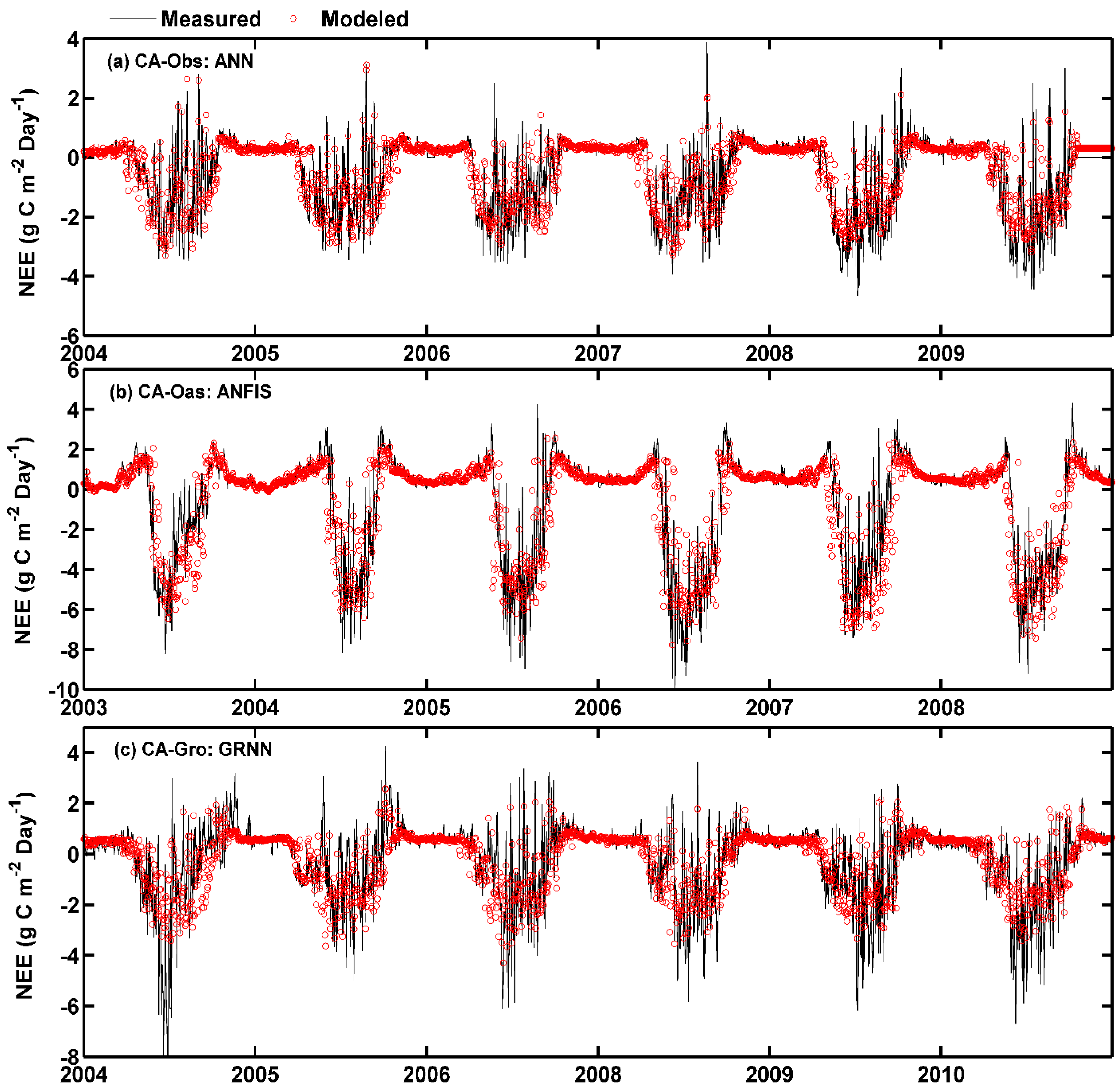
On the other hand, the over- and under-estimation of the best model in predicting the daily NEE for the three sites among the training, validation and testing periods are illustrated in Figure 6. It is clear that most of the estimated values closely follow the corresponding observed values in the three stands. In the growing season, however, the NEE values simulated by the GRNN model at CA-Gro site fail to well match the corresponding measured values.
3.4. Modeling of Hourly Carbon Fluxes
To examine the modeling ability of machine learning methods at a finer time scale, we further use these approaches to estimate hourly carbon fluxes at the three sites. The results estimated by different models with four input variables in the testing period are shown in Table 9. It should be noted that the gap-filled hourly carbon flux data were not used for these estimates. The number of observed NEE data available in the testing period in Table 9 is 5865 (2009), 6233 (2008) and 6099 (2010) for CA-Obs, CA-Oas and CA-Gro, respectively. As a whole, the machine learning models accurately quantify hourly carbon fluxes at the three sites. They consistently and substantially outperform the MLR model for GPP and NEE estimates in terms of R2, NSE, Bias and RMSE, while for R estimates, the MLR model achieves satisfactory results comparable to those of machine learning models. Specifically, for the comparison among the three sites in the prediction of hourly GPP, the developed machine learning models offered the highest accuracy at CA-Obs site, followed by CA-Oas site. Regarding the estimates of hourly R among the three sites, according to the R2 indictor, the applied models perform the best at CA-Gro site, whereas they provide the worst statistical results with respect to NSE, Bias and RMSE indices. On the whole, these models generate the best R estimates in terms of NSE, Bias and RMSE. For NEE estimates, the machine learning models give similar results at both CA-Obs and CA-Oas sites, and slightly perform better than the models at CA-Gro site.
As commonly known in the eddy covariance community, the requirement for turbulent atmospheric conditions limits the quality of data observed by the eddy covariance technique. Half-hourly NEE data are directly measured and may be rejected due to low turbulence conditions. The majority of missing NEE data occur during nighttime. Therefore, it is essential to provide some insights into the modeling ability of our proposed models for nighttime and daytime NEE data. In this study, the identification of nighttime and daytime was according to the values of photosynthetic photon flux density (PPFD). A positive PPFD implied daytime, while nighttime was defined by the periods of the day without light (the values of PPFD were equal to zero). The comparisons of different models with four input variables for predicting hourly NEE in the testing period for daytime and nighttime datasets at the three sites are summarized in Table 10. As can be seen from the Table 9 and Table 10, the NEE estimates of each model for the daytime data at both CA-Obs and CA-Oas sites are similar to those for all the data (daytime + nighttime), and are considerably better than those for the nighttime data. In contrast, at CA-Gro site, all the models (except MLR) for the daytime and nighttime data give similar estimates according to the R2 performance index (Table 10), while in terms of the NSE index, the estimates from all the models for the daytime data are consistently superior to those for the nighttime data.
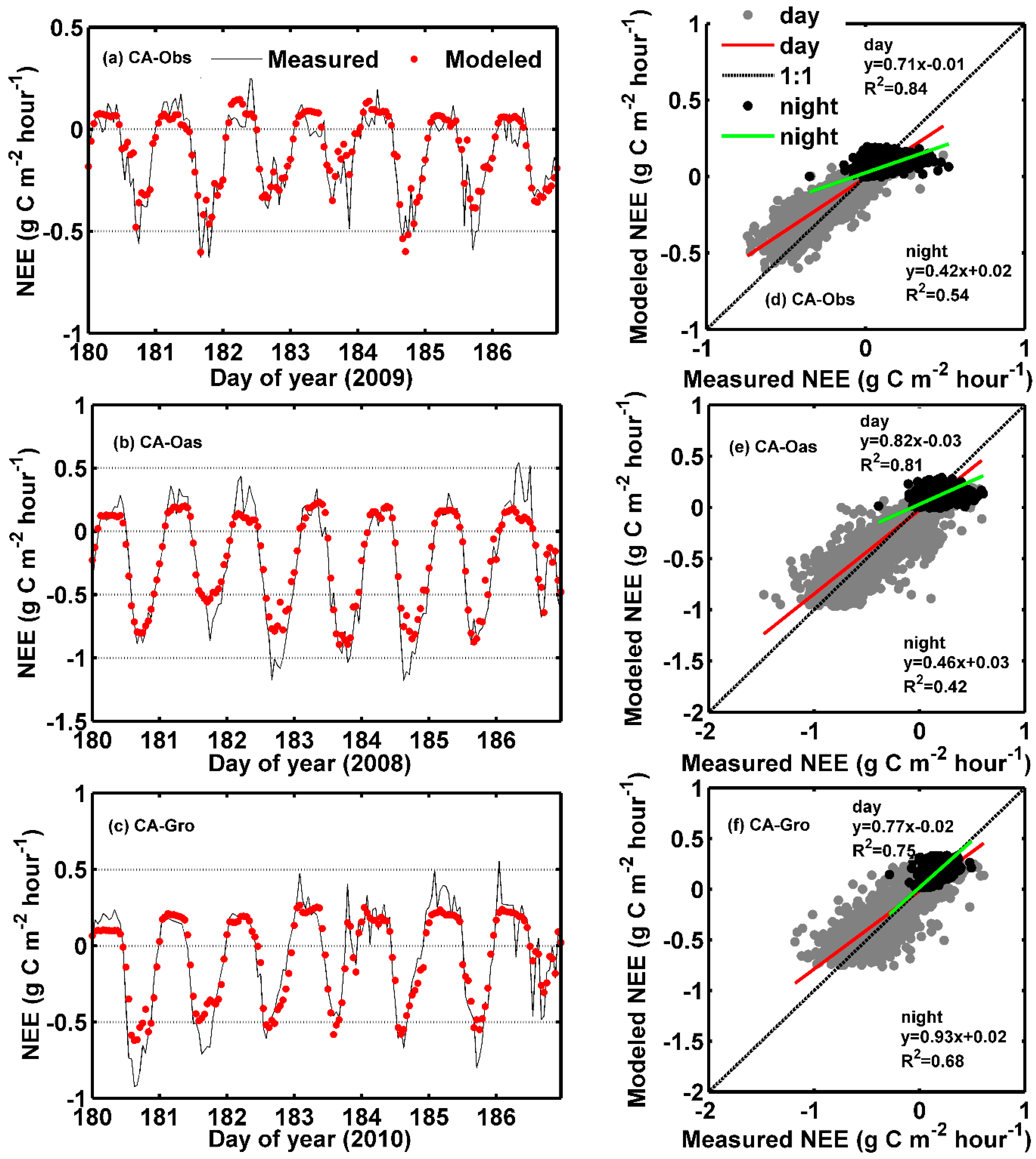
As a case study, Figure 7 illustrates hourly NEE between eddy covariance measured and predicted by the ANFIS model in the testing period. The daily courses of hourly measured and predicted NEE flux for 7 days during the mid-growing season at the three sites are displayed in Figure 7a–c. It can be clearly seen that most of the modeled NEE values at the three sites well match the corresponding observed ones. In comparison with the estimates at both CA-Oas and CA-Gro sites, the simulated NEE values at CA-Obs site more closely match the corresponding measured ones. The scatter plots of ANFIS modeled and measured hourly NEE flux for both nighttime and daytime datasets at the three sites are presented in Figure 7d–f. As shown in the figures, considerable difference between nighttime and daytime datasets can be found in the magnitude and variation of hourly NEE for an entire testing year, which are largely reduced during nighttime primarily due to the absence of photosynthesis. For the daytime datasets among the three sites, the fit line of the ANFIS model at CA-Oas site is closest to the ideal straight line of slope one, while this model have the highest value of R2 at CA-Obs site. However, for the nighttime datasets among the three sites, the best estimates occur at CA-Gro site in terms of both the slope of the fit line and R2 value.
4. Discussion
For the first time, the suitability and potential of two advanced machine learning techniques, namely ANFIS and GRNN, were investigated in the prediction of terrestrial carbon fluxes using the EC-measured data in three forest ecosystems. Besides, another three traditional approaches (ANN, SVM and MLR) were also used as benchmarks in order to evaluate the modeling capability of all the applied models in the present study. In the following subsections, we primarily focused on discussing the estimates of carbon fluxes among the machine learning models, according to the different performance evaluation indices. In addition, we also provided the advantages and limitations of the present research, as well as the possible improvements in the future work.
4.1. Capability of Machine Learning Models and Their Comparison
Our results demonstrated that the applied machine learning models with full input variables (Ta, Rn, Rh, Ts) did an excellent job of explaining approximately average 92%, 94% and 78% of diurnal variances in GPP, R and NEE for the three stands, respectively (Table 5). These models also exhibited great capability in mapping the hourly variation of different carbon fluxes in response to environmental factors. According to the estimates of each method with different input combinations (Table 4, Table 7 and Table 8), it is clear that the relative importance of driving variables is different with respect to each carbon flux. More specifically, the contributions of Ta and Ts in estimating daily GPP are similar and more than those of Rn and Rh at the three sites. Ts is the most predominant factor controlling the variability of R flux at each site, followed by Ta and then Rn. However, considerable difference among the three forest sites was found in the contributions of these driving variables to NEE. At CA-Obs site, Ta and Rn provided similar contributions and played more important role than Ts and Rh; At CA-Oas site, Ts offered the largest contribution to NEE, followed by Ta and then Rn; The largest contribution to NEE at CA-Gro site was from Rn, followed by Ts and then Ta. Overall, the contribution of Rh to each carbon flux at the three sites was relatively lower, compared with the other three variables.
In addition, these advanced machine learning models consistently performed better than the traditional MLR model for each carbon flux prediction. The predictive performance of these techniques at various terrestrial ecosystems was also confirmed by previous studies, mainly involving ANN and SVM approaches [12,21,47]. Additionally, it is worth mentioning here that both ANN and SVM machine learning techniques in recent years have been extensively accepted as preferred tools to upscale the terrestrial carbon fluxes from site to regional scale [13,20,48,49]. More importantly, previous studies have pointed out that, based on the data derived from the remote sensing and EC techniques, data-driven models can perform better than land surface models for predicting the terrestrial carbon fluxes at regional and global scales [50,51].
Furthermore, regarding all the examined machine learning models, our results revealed that these models can consistently estimate hourly and daily carbon fluxes at the three sites (Table 5 and Table 9). Specifically, conventional ANN method remains adequately competent in reproducing the carbon fluxes due to its strong generalization ability. For this reason, recently, it has been continuously utilized in the estimation of carbon fluxes [22,52,53]. In addition, ANFIS, as a state of the art method, is designed by combining the strength of FIS and adaptive neural networks for the purpose of identifying the beneficial knowledge within the trained networks in the form of fuzzy logic expression. Therefore, ANFIS seems to be able to overcome the weakness of knowledge interpretation which is still a great challenge for neural networks. In theory at least, ANFIS could perform better than ANN method and this assumption has been proved by many previous studies in practical terms [54,55]. However, in the present work, our results showed that ANFIS and ANN produced the similar estimates, which concurs with the results of both Karimi et al. [56] and Piri et al. [57] for the hydrological time series forecasting. A potential reason for the difference can be accounted for by the fact that the generalization capability of ANFIS is hugely influenced by FIS with various identification algorithms [45,58], indicating that other identification algorithms for generating a FIS, such as fuzzy c-means, mountain, and grid partitioning, may enhance the modeling performance of ANFIS method for the current research.
Moreover, in order to improve the predictive ability of data-driven techniques, packaging heuristic algorithms into data-driven models with the intention of optimizing the model structures and/or parameters is broadly adopted as a preferred solution. A large number of novel nature-inspired optimization algorithms (e.g., particle swarm optimization [59], artificial bee colony [60] and cuckoo search optimization [61]) have been developed over the last two decades [62]. It should be particularly stressed that the models developed in this study have been successfully optimized by various heuristic algorithms in diverse research fields (e.g., hydrological prediction, wind speed and solar radiation forecasting). For instance, Baghban et al. [63] used genetic algorithm to tune, optimize, and determine the respective key parameters of ANFIS and SVM methods for predicting the dew point temperature of moist air and obtained excellent results; Moosavi et al. [64] utilized particle swarm optimization algorithm in conjunction with ANFIS and SVM approaches to estimate the surface soil moisture and respectively improved the predictive performance of original ANFIS and SVM models without using optimization algorithm. Consequently, to improve the modeling accuracy of carbon fluxes in the present work, further studies can be devoted to optimizing the machine learning models by the aid of different meta-heuristic algorithms.
4.2. Advantages and Limitations of Present Research and Future Work
We modelled the carbon fluxes at three different forest ecosystems using four different modeling techniques. The ability of these techniques has been demonstrated in terms of dealing with the nonlinear processes that control the daily carbon fluxes. In general, the best predictive results for the three carbon fluxes were provided at the evergreen needle-leaf forest (CA-Obs), followed by the deciduous broadleaf forest (CA-Oas), whereas the worst performance was obtained at the mixed forest (CA-Gro), maybe due to the difficulty for our proposed models in seizing the useful knowledge resulting from the influences of more complex and instable underlying surface (Table 6). Moreover, this performance difference among the three sites may be due to the climate extreme events. For instance, at CA-Gro site, compared with the 4-year means over the training period, the annual average values of Rn, Ts and Ta and in the testing period were higher by about 0.2 mol m−2, 0.2 °C and 1.6 °C, respectively. These three variables have been found to be the most important driving factors dominating the variation of carbon fluxes (Table 4, Table 7 and Table 8). On the other hand, for each estimated flux at all the three forest ecosystems, our applied models generally produced satisfactory results (Table 5 and Table 6), especially for GPP and R fluxes. In addition, more remarkable difference among the three fluxes was that the predictive results of both GPP and R were substantially superior to those of NEE, which is in accordance with the previous studies [22,65]. As a matter of fact, NEE, as a balance between GPP and R fluxes, is controlled by the interplay of assimilation and respiration processes between the biosphere and the atmosphere, and this interplay highly influences the diurnal, seasonal and inter-annual variations in NEE involving amplitude and phase [66]. Consequently, accurately estimating NEE remains a great challenge for the researchers to date.
Furthermore, it is a generally acknowledged fact that pursuing excessively the convenience and simplification of the used models may cause the under-fitting for the trained models. In our study, a possible reason for the lower explanation of NEE from the applied models seems to be the missing of some key driving variables for model design, such as biomass pools and management activities. Therefore, in the follow-up work, the sensitivity analysis of a variety of variables in relation to carbon fluxes (particularly for NEE), as well as the addition of effective driving variables as model inputs should be further investigated to improve the predictive performance of our proposed models for the carbon flux forecasting. On the other hand, NEE measurements have been extensively used for estimating carbon budgets at different spatial and temporal scales. Therefore, data gaps in NEE measured by EC technique must be precisely filled [19,67]. However, no standard gap-filling approach for CO2 flux time series data with the EC method has been widely accepted [15,68]. Consequently, it is of importance to identify optimal filling approaches for accurately determining carbon budgets. According to the present estimates, our proposed methods could be used as useful alternatives to address the problem of gap-filling in EC measurements in the future.
In practical terms, our study presented the performance difference among the utilized models and also found that the instability of the data-driven models in terms of predictive accuracy for each case indeed existed (Table 5, Table 9 and Table 10). To obtain more stable model as well as better predictive accuracy, a novel technique, namely ensemble learning, has gained extensive attention in recent years [69,70]. The purpose of ensemble learning is to combine the positive properties of a diverse set of learners generated from either the same or different machine learning methods. Apart from the applied methods, the performance of ensemble learning generally varies depending on both the generation of input data from the whole sample and the integration of various learners for the final output. At present, many studies focus on the ensemble generation approaches for inputs of different learners, mainly including bagging [71], boosting [72], and random forests [73]. These algorithms can be combined with machine learning methods for producing more accurate solution than an individual method, which has been proved by previous studies both in theory and practice [74,75]. For example, for the water quality forecasting, Barzegar et al. [76] reported that a boosting algorithm in conjunction with wavelet-based ELM and wavelet-based ANFIS models performed better than their respective single models without using the ensemble technique, respectively. Keenan et al. [77] found the variability in predictive capability among nine different machine learning approaches for estimating the species distributions in three forest stands and obtained a better predictive results through multiple model ensemble technique. To our best knowledge, the suitability and ability of ensemble learning techniques have never been explored for carbon flux forecasting research. Therefore, it may be effective to enhance the performance of our applied models in terms of stability and predictability for the present study. However, it is beyond the scope of the current investigation and will be undertaken in our follow-up work.
5. Conclusions
This study focused on investigating the feasibility and potential of both the GRNN and ANFIS models for modeling and forecasting daily carbon fluxes in three different forest ecosystems. Moreover, their predictive accuracy was compared with traditional ANN, SVM and MLR models. All the models were evaluated according to several performance indicators (R2, NSE, Bias and RMSE). It has been found that all the machine learning models proposed in this study, including ANN, GRNN, ANFIS and SVM, were capable of accounting for the most variance in each carbon flux at both daily and hourly time scales in the three stands, especially for both GPP and R. These modern models consistently performed better than conventional MLR model for both daily and hourly carbon flux estimates in terms of R2, NSE, Bias and RMSE. Therefore, these advanced models were able to elucidate precisely non-linear processes of controlling the exchanges of the carbon fluxes between land and the atmosphere at the ecosystem level. Moreover, among all the applied models, the ANFIS and ANN models provided similar estimates of carbon fluxes and slightly outperformed the GRNN and SVM models. In practical terms, however, the ANFIS and GRNN models are more robust and flexible, and have less parameters needed for selection and optimization, when compared with two common ANN and SVM models. Accordingly, both the ANFIS and GRNN models are valuable tools for estimating forest carbon fluxes and interpolating the missing carbon flux data during the long-term EC measurements.
Considering the findings above, our study has conclusively demonstrated for the first time that both the ANFIS and GRNN models can effectively reproduce carbon fluxes at the ecosystem level. Consequently, when upscaling the carbon and water fluxes from ecosystem to regional or global scale, these promising tools should be taken into consideration, which is comparatively important for the scientific community to determine the global carbon and water budgets and offer reliable information for policy makers responding to global climate change.
Acknowledgments
The work was financially supported by the Natural Science Fund of China (No. 41672324, No. 41430317 and No. 41402291), the National Science and Technology Major Projects (No. 2016ZX05044-002), and the Priority Academic Program Development of Jiangsu Higher Education Institutions. The present study used the EC measurements acquired and shared by the Fluxnet-Canada Research Network and FLUXNET community. The authors acknowledge all the project investigators and their staff and graduate students for providing the flux data. The authors also gratefully acknowledge three anonymous reviewers for their constructive comments.
Author Contributions
Yongguo Yang and Xianming Dou conceived and designed the experiments; Xianming Dou performed the experiments, analyzed the data and wrote the manuscript; Yongguo Yang and Jinhui Luo provided important suggestions for the final manuscript.
Conflicts of Interest
The authors declare no conflict of interest.
References
- Pan, Y.; Birdsey, R.A.; Fang, J.; Houghton, R.; Kauppi, P.E.; Kurz, W.A.; Phillips, O.L.; Shvidenko, A.; Lewis, S.L.; Canadell, J.G. A large and persistent carbon sink in the world’s forests. Science 2011, 333, 988–993. [Google Scholar] [CrossRef] [PubMed]
- Malhi, Y.; Baldocchi, D.D.; Jarvis, P.G. The carbon balance of tropical, temperate and boreal forests. Plant Cell Environ. 1999, 22, 715–740. [Google Scholar] [CrossRef]
- Alkama, R.; Cescatti, A. Biophysical climate impacts of recent changes in global forest cover. Science 2016, 351, 600–604. [Google Scholar] [CrossRef] [PubMed] [Green Version]
- Anderegg, W.R.; Schwalm, C.; Biondi, F.; Camarero, J.J.; Koch, G.; Litvak, M.; Ogle, K.; Shaw, J.D.; Shevliakova, E.; Williams, A. Pervasive drought legacies in forest ecosystems and their implications for carbon cycle models. Science 2015, 349, 528–532. [Google Scholar] [CrossRef] [PubMed]
- Tang, Y.; Wen, X.; Sun, X.; Chen, Y.; Wang, H. Contribution of environmental variability and ecosystem functional changes to interannual variability of carbon and water fluxes in a subtropical coniferous plantation. iForest Biogeosci. For. 2016, 9, 452–460. [Google Scholar] [CrossRef]
- Clark, J.S.; Iverson, L.; Woodall, C.W.; Allen, C.D.; Bell, D.M.; Bragg, D.C.; D’Amato, A.W.; Davis, F.W.; Hersh, M.H.; Ibanez, I.; et al. The impacts of increasing drought on forest dynamics, structure, and biodiversity in the united states. Glob. Chang. Biol. 2016, 22, 2329–2352. [Google Scholar] [CrossRef] [PubMed]
- Schindler, D.E.; Hilborn, R. Prediction, precaution, and policy under global change. Science 2015, 347, 953–954. [Google Scholar] [CrossRef] [PubMed]
- Ye, H.; Beamish, R.J.; Glaser, S.M.; Grant, S.C.H.; Hsieh, C.-H.; Richards, L.J.; Schnute, J.T.; Sugihara, G. Equation-free mechanistic ecosystem forecasting using empirical dynamic modeling. Proc. Natl. Acad. Sci. USA 2015, 112, E1569–E1576. [Google Scholar] [CrossRef] [PubMed]
- Schmidt, A.; Wrzesinsky, T.; Klemm, O. Gap filling and quality assessment of CO2 and water vapour fluxes above an urban area with radial basis function neural networks. Boundary-Layer Meteorol. 2008, 126, 389–413. [Google Scholar] [CrossRef]
- Braswell, B.H.; Sacks, W.J.; Linder, E.; Schimel, D.S. Estimating diurnal to annual ecosystem parameters by synthesis of a carbon flux model with eddy covariance net ecosystem exchange observations. Glob. Chang. Biol. 2005, 11, 335–355. [Google Scholar] [CrossRef]
- Menzer, O.; Moffat, A.M.; Meiring, W.; Lasslop, G.; Schukat-Talamazzini, E.G.; Reichstein, M. Random errors in carbon and water vapor fluxes assessed with gaussian processes. Agric. For. Meteorol. 2013, 178, 161–172. [Google Scholar] [CrossRef]
- Moffat, A.M.; Beckstein, C.; Churkina, G.; Mund, M.; Heimann, M. Characterization of ecosystem responses to climatic controls using artificial neural networks. Glob. Chang. Biol. 2010, 16, 2737–2749. [Google Scholar] [CrossRef]
- Papale, D.; Valentini, R. A new assessment of european forests carbon exchanges by eddy fluxes and artificial neural network spatialization. Glob. Chang. Biol. 2003, 9, 525–535. [Google Scholar] [CrossRef]
- Moffat, A.M.; Papale, D.; Reichstein, M.; Hollinger, D.Y.; Richardson, A.D.; Barr, A.G.; Beckstein, C.; Braswell, B.H.; Churkina, G.; Desai, A.R.; et al. Comprehensive comparison of gap-filling techniques for eddy covariance net carbon fluxes. Agric. For. Meteorol. 2007, 147, 209–232. [Google Scholar] [CrossRef]
- Ooba, M.; Hirano, T.; Mogami, J.-I.; Hirata, R.; Fujinuma, Y. Comparisons of gap-filling methods for carbon flux dataset: A combination of a genetic algorithm and an artificial neural network. Ecol. Model. 2006, 198, 473–486. [Google Scholar] [CrossRef]
- Wang, T.; Brender, P.; Ciais, P.; Piao, S.; Mahecha, M.D.; Chevallier, F.; Reichstein, M.; Ottlé, C.; Maignan, F.; Arain, A.; et al. State-dependent errors in a land surface model across biomes inferred from eddy covariance observations on multiple timescales. Ecol. Model. 2012, 246, 11–25. [Google Scholar] [CrossRef]
- Abramowitz, G.; Pitman, A.; Gupta, H.; Kowalczyk, E.; Wang, Y. Systematic bias in land surface models. J. Hydrometeorol. 2007, 8, 989–1001. [Google Scholar] [CrossRef]
- Papale, D.; Black, T.A.; Carvalhais, N.; Cescatti, A.; Chen, J.; Jung, M.; Kiely, G.; Lasslop, G.; Mahecha, M.D.; Margolis, H.; et al. Effect of spatial sampling from european flux towers for estimating carbon and water fluxes with artificial neural networks. J. Geophys. Res. Biogeosci. 2015, 120, 1941–1957. [Google Scholar] [CrossRef]
- Ueyama, M.; Ichii, K.; Iwata, H.; Euskirchen, E.S.; Zona, D.; Rocha, A.V.; Harazono, Y.; Iwama, C.; Nakai, T.; Oechel, W.C. Upscaling terrestrial carbon dioxide fluxes in alaska with satellite remote sensing and support vector regression. J. Geophys. Res. Biogeosci. 2013, 118, 1266–1281. [Google Scholar] [CrossRef]
- Yang, F.; Ichii, K.; White, M.A.; Hashimoto, H.; Michaelis, A.R.; Votava, P.; Zhu, A.X.; Huete, A.; Running, S.W.; Nemani, R.R. Developing a continental-scale measure of gross primary production by combining modis and ameriflux data through support vector machine approach. Remote Sens. Environ. 2007, 110, 109–122. [Google Scholar] [CrossRef]
- Melesse, A.M.; Hanley, R.S. Artificial neural network application for multi-ecosystem carbon flux simulation. Ecol. Model. 2005, 189, 305–314. [Google Scholar] [CrossRef]
- Dou, X.; Chen, B.; Black, T.; Jassal, R.; Che, M. Impact of nitrogen fertilization on forest carbon sequestration and water loss in a chronosequence of three douglas-fir stands in the pacific northwest. Forests 2015, 6, 1897–1921. [Google Scholar] [CrossRef]
- Evrendilek, F. Assessing CO2 sink/source strength of a degraded temperate peatland: Atmospheric and hydrological drivers and responses to extreme events. Ecohydrology 2015, 8, 1429–1445. [Google Scholar] [CrossRef]
- Ladlani, I.; Houichi, L.; Djemili, L.; Heddam, S.; Belouz, K. Modeling daily reference evapotranspiration (ET0) in the north of algeria using generalized regression neural networks (GRNN) and radial basis function neural networks (RBFNN): A comparative study. Meteorol. Atmos. Phys. 2012, 118, 163–178. [Google Scholar] [CrossRef]
- Petković, D.; Gocic, M.; Trajkovic, S.; Shamshirband, S.; Motamedi, S.; Hashim, R.; Bonakdari, H. Determination of the most influential weather parameters on reference evapotranspiration by adaptive neuro-fuzzy methodology. Comput. Electron. Agric. 2015, 114, 277–284. [Google Scholar] [CrossRef]
- Kim, S.; Shiri, J.; Kisi, O.; Singh, V.P. Estimating daily pan evaporation using different data-driven methods and lag-time patterns. Water Resour. Manag. 2013, 27, 2267–2286. [Google Scholar] [CrossRef]
- Shiri, J.; Dierickx, W.; Pour-Ali Baba, A.; Neamati, S.; Ghorbani, M.A. Estimating daily pan evaporation from climatic data of the state of Illinois, USA using adaptive neuro-fuzzy inference system (ANFIS) and artificial neural network (ANN). Hydrol. Res. 2011, 42, 491. [Google Scholar] [CrossRef]
- Chitsaz, N.; Azarnivand, A.; Araghinejad, S. Pre-processing of data-driven river flow forecasting models by singular value decomposition (SVD) technique. Hydrol. Sci. J. 2016, 61, 2164–2178. [Google Scholar] [CrossRef]
- Kisi, O.; Nia, A.M.; Gosheh, M.G.; Tajabadi, M.R.J.; Ahmadi, A. Intermittent streamflow forecasting by using several data driven techniques. Water Resour. Manag. 2012, 26, 457–474. [Google Scholar] [CrossRef]
- Shirmohammadi, B.; Vafakhah, M.; Moosavi, V.; Moghaddamnia, M. Application of several data-driven techniques for predicting groundwater level. Water Resour. Manag. 2013, 27, 419–432. [Google Scholar] [CrossRef]
- Moosavi, V.; Vafakhah, M.; Shirmohammadi, B.; Behnia, N. A wavelet-anfis hybrid model for groundwater level forecasting for different prediction periods. Water Resour. Manag. 2013, 27, 1301–1321. [Google Scholar] [CrossRef]
- Jang, J.-S. Anfis: Adaptive-network-based fuzzy inference system. IEEE Trans. Syst. Man Cybern. 1993, 23, 665–685. [Google Scholar] [CrossRef]
- Specht, D.F. A general regression neural network. IEEE Trans. Neural Netw. 1991, 2, 568–576. [Google Scholar] [CrossRef] [PubMed]
- Zha, T.; Barr, A.G.; van der Kamp, G.; Black, T.A.; McCaughey, J.H.; Flanagan, L.B. Interannual variation of evapotranspiration from forest and grassland ecosystems in western canada in relation to drought. Agric. For. Meteorol. 2010, 150, 1476–1484. [Google Scholar] [CrossRef]
- Griffis, T.J.; Black, T.A.; Morgenstern, K.; Barr, A.G.; Nesic, Z.; Drewitt, G.B.; Gaumont-Guay, D.; McCaughey, J.H. Ecophysiological controls on the carbon balances of three southern boreal forests. Agric. For. Meteorol. 2003, 117, 53–71. [Google Scholar] [CrossRef]
- Krishnan, P.; Black, T.A.; Barr, A.G.; Grant, N.J.; Gaumont-Guay, D.; Nesic, Z. Factors controlling the interannual variability in the carbon balance of a southern boreal black spruce forest. J. Geophys. Res. 2008, 113. [Google Scholar] [CrossRef]
- McCaughey, J.H.; Pejam, M.R.; Arain, M.A.; Cameron, D.A. Carbon dioxide and energy fluxes from a boreal mixedwood forest ecosystem in ontario, canada. Agric. For. Meteorol. 2006, 140, 79–96. [Google Scholar] [CrossRef]
- Barr, A.G.; Black, T.A.; Hogg, E.H.; Griffis, T.J.; Morgenstern, K.; Kljun, N.; Theede, A.; Nesic, Z. Climatic controls on the carbon and water balances of a boreal aspen forest, 1994–2003. Glob. Chang. Biol. 2007, 13, 561–576. [Google Scholar] [CrossRef]
- Ata, R. Artificial neural networks applications in wind energy systems: A review. Renew. Sustain. Energy Rev. 2015, 49, 534–562. [Google Scholar] [CrossRef]
- Yadav, A.K.; Chandel, S.S. Solar radiation prediction using artificial neural network techniques: A review. Renew. Sustain. Energy Rev. 2014, 33, 772–781. [Google Scholar] [CrossRef]
- Maier, H.R.; Jain, A.; Dandy, G.C.; Sudheer, K.P. Methods used for the development of neural networks for the prediction of water resource variables in river systems: Current status and future directions. Environ. Model. Softw. 2010, 25, 891–909. [Google Scholar] [CrossRef]
- Vapnik, V.N. An overview of statistical learning theory. IEEE Trans. Neural Netw. 1999, 10, 988–999. [Google Scholar] [CrossRef] [PubMed]
- Takagi, T.; Sugeno, M. Fuzzy identification of systems and its applications to modeling and control. IEEE Trans. Syst. Man Cybern. 1985, SMC-15, 116–132. [Google Scholar] [CrossRef]
- Mamdani, E.H.; Assilian, S. An experiment in linguistic synthesis with a fuzzy logic controller. Int. J. Man-Mach. Stud. 1975, 7, 1–13. [Google Scholar] [CrossRef]
- Cobaner, M. Evapotranspiration estimation by two different neuro-fuzzy inference systems. J. Hydrol. 2011, 398, 292–302. [Google Scholar] [CrossRef]
- Kisi, O. The potential of different ann techniques in evapotranspiration modelling. Hydrol. Process. 2008, 22, 2449–2460. [Google Scholar] [CrossRef]
- Evrendilek, F. Assessing neural networks with wavelet denoising and regression models in predicting diel dynamics of eddy covariance-measured latent and sensible heat fluxes and evapotranspiration. Neural Comput. Appl. 2012, 24, 327–337. [Google Scholar] [CrossRef]
- Kondo, M.; Ichii, K.; Takagi, H.; Sasakawa, M. Comparison of the data-driven top-down and bottom-up global terrestrial CO2 exchanges: Gosat CO2 inversion and empirical eddy flux upscaling. J. Geophys. Res. Biogeosci. 2015, 120, 1226–1245. [Google Scholar] [CrossRef]
- Beer, C.; Reichstein, M.; Tomelleri, E.; Ciais, P.; Jung, M.; Carvalhais, N.; Rödenbeck, C.; Arain, M.A.; Baldocchi, D.; Bonan, G.B. Terrestrial gross carbon dioxide uptake: Global distribution and covariation with climate. Science 2010, 329, 834–838. [Google Scholar] [CrossRef] [PubMed]
- Anav, A.; Friedlingstein, P.; Beer, C.; Ciais, P.; Harper, A.; Jones, C.; Murray-Tortarolo, G.; Papale, D.; Parazoo, N.C.; Peylin, P.; et al. Spatiotemporal patterns of terrestrial gross primary production: A review. Rev. Geophys. 2015, 53, 785–818. [Google Scholar] [CrossRef] [Green Version]
- Huntzinger, D.N.; Post, W.M.; Wei, Y.; Michalak, A.M.; West, T.O.; Jacobson, A.R.; Baker, I.T.; Chen, J.M.; Davis, K.J.; Hayes, D.J.; et al. North american carbon program (NACP) regional interim synthesis: Terrestrial biospheric model intercomparison. Ecol. Model. 2012, 232, 144–157. [Google Scholar] [CrossRef]
- Liu, S.; Zhuang, Q.; He, Y.; Noormets, A.; Chen, J.; Gu, L. Evaluating atmospheric CO2 effects on gross primary productivity and net ecosystem exchanges of terrestrial ecosystems in the conterminous united states using the ameriflux data and an artificial neural network approach. Agric. For. Meteorol. 2016, 220, 38–49. [Google Scholar] [CrossRef]
- Sulkava, M.; Luyssaert, S.; Zaehle, S.; Papale, D. Assessing and improving the representativeness of monitoring networks: The european flux tower network example. J. Geophys. Res. Biogeosci. 2011, 116, G00J04. [Google Scholar] [CrossRef]
- Kurtulus, B.; Razack, M. Modeling daily discharge responses of a large karstic aquifer using soft computing methods: Artificial neural network and neuro-fuzzy. J. Hydrol. 2010, 381, 101–111. [Google Scholar] [CrossRef]
- Emamgholizadeh, S.; Moslemi, K.; Karami, G. Prediction the groundwater level of bastam plain (Iran) by artificial neural network (ANN) and adaptive neuro-fuzzy inference system (ANFIS). Water Resour. Manag. 2014, 28, 5433–5446. [Google Scholar] [CrossRef]
- Karimi, S.; Kisi, O.; Shiri, J.; Makarynskyy, O. Neuro-fuzzy and neural network techniques for forecasting sea level in darwin harbor, Australia. Comput. Geosci. 2013, 52, 50–59. [Google Scholar] [CrossRef]
- Piri, J.; Mohammadi, K.; Shamshirband, S.; Akib, S. Assessing the suitability of hybridizing the cuckoo optimization algorithm with ann and anfis techniques to predict daily evaporation. Environ. Earth Sci. 2016, 75, 246. [Google Scholar] [CrossRef]
- Mollaiy-Berneti, S. Optimal design of adaptive neuro-fuzzy inference system using genetic algorithm for electricity demand forecasting in iranian industry. Soft Comput. 2015, 20, 4897–4906. [Google Scholar] [CrossRef]
- Poli, R. Analysis of the publications on the applications of particle swarm optimisation. J. Artif. Evolut. Appl. 2008, 2008, 685175. [Google Scholar] [CrossRef]
- Karaboga, D.; Basturk, B. A powerful and efficient algorithm for numerical function optimization: Artificial bee colony (ABC) algorithm. J. Glob. Optim. 2007, 39, 459–471. [Google Scholar] [CrossRef]
- Yang, X.-S.; Deb, S. Engineering optimisation by cuckoo search. Int. J. Math. Model. Numer. Optim. 2010, 1, 330–343. [Google Scholar] [CrossRef]
- Parpinelli, R.S.; Lopes, H.S. New inspirations in swarm intelligence: A survey. Int. J. Bio-Inspir. Comput. 2011, 3, 1–16. [Google Scholar] [CrossRef]
- Baghban, A.; Bahadori, M.; Rozyn, J.; Lee, M.; Abbas, A.; Bahadori, A.; Rahimali, A. Estimation of air dew point temperature using computational intelligence schemes. Appl. Therm. Eng. 2016, 93, 1043–1052. [Google Scholar] [CrossRef]
- Moosavi, V.; Talebi, A.; Mokhtari, M.H.; Hadian, M.R. Estimation of spatially enhanced soil moisture combining remote sensing and artificial intelligence approaches. Int. J. Remote Sens. 2016, 37, 5605–5631. [Google Scholar] [CrossRef]
- Tramontana, G.; Jung, M.; Schwalm, C.R.; Ichii, K.; Camps-Valls, G.; Ráduly, B.; Reichstein, M.; Arain, M.A.; Cescatti, A.; Kiely, G.; et al. Predicting carbon dioxide and energy fluxes across global fluxnet sites with regression algorithms. Biogeosciences 2016, 13, 4291–4313. [Google Scholar] [CrossRef] [Green Version]
- Stoy, P.; Richardson, A.; Baldocchi, D.; Katul, G.; Stanovick, J.; Mahecha, M.; Reichstein, M.; Detto, M.; Law, B.; Wohlfahrt, G. Biosphere-atmosphere exchange of CO2 in relation to climate: A cross-biome analysis across multiple time scales. Biogeosciences 2009, 6, 2297–2312. [Google Scholar] [CrossRef]
- Soloway, A.D.; Amiro, B.D.; Dunn, A.L.; Wofsy, S.C. Carbon neutral or a sink? Uncertainty caused by gap-filling long-term flux measurements for an old-growth boreal black spruce forest. Agric. For. Meteorol. 2017, 233, 110–121. [Google Scholar] [CrossRef]
- Dragomir, C.M.; Klaassen, W.; Voiculescu, M.; Georgescu, L.P.; van der Laan, S. Estimating annual CO2 flux for lutjewad station using three different gap-filling techniques. Sci. World J. 2012, 2012, 842893. [Google Scholar] [CrossRef] [PubMed]
- Dietterich, T.G. Ensemble learning. In The Handbook of Brain Theory and Neural Networks; The MIT Press: Cambridge, MA, USA, 2002; Volume 2, pp. 110–125. [Google Scholar]
- Zhou, Z.-H. Ensemble learning. Encycl. Biom. 2015, 411–416. [Google Scholar] [CrossRef]
- Breiman, L. Bagging predictors. Mach. Learn. 1996, 24, 123–140. [Google Scholar] [CrossRef]
- Freund, Y.; Schapire, R.; Abe, N. A short introduction to boosting. J. Jpn. Soc. For. Artif. Intell. 1999, 14, 771–780. [Google Scholar]
- Breiman, L. Random forests. Mach. Learn. 2001, 45, 5–32. [Google Scholar] [CrossRef]
- Bauer, E.; Kohavi, R. An empirical comparison of voting classification algorithms: Bagging, boosting, and variants. Mach. Learn. 1999, 36, 105–139. [Google Scholar] [CrossRef]
- Strobl, C.; Malley, J.; Tutz, G. An introduction to recursive partitioning: Rationale, application, and characteristics of classification and regression trees, bagging, and random forests. Psychol. Methods 2009, 14, 323–348. [Google Scholar] [CrossRef] [PubMed] [Green Version]
- Barzegar, R.; Moghaddam, A.A.; Adamowski, J.; Ozga-Zielinski, B. Multi-step water quality forecasting using a boosting ensemble multi-wavelet extreme learning machine model. Stoch. Environ. Res. Risk Assess. 2017, 1–15. [Google Scholar] [CrossRef]
- Keenan, T.; Maria Serra, J.; Lloret, F.; Ninyerola, M.; Sabate, S. Predicting the future of forests in the mediterranean under climate change, with niche- and process-based models: CO2 matters! Glob. Chang. Biol. 2011, 17, 565–579. [Google Scholar] [CrossRef]
Figure 1.
Comparisons of measured and simulated daily gross primary productivity (GPP) in the testing period in the three boreal forest stands. (a–e) For CA-Obs stand; (f–j) for CA-Oas stand; and (k–o) for CA-Gro stand.
Figure 1.
Comparisons of measured and simulated daily gross primary productivity (GPP) in the testing period in the three boreal forest stands. (a–e) For CA-Obs stand; (f–j) for CA-Oas stand; and (k–o) for CA-Gro stand.
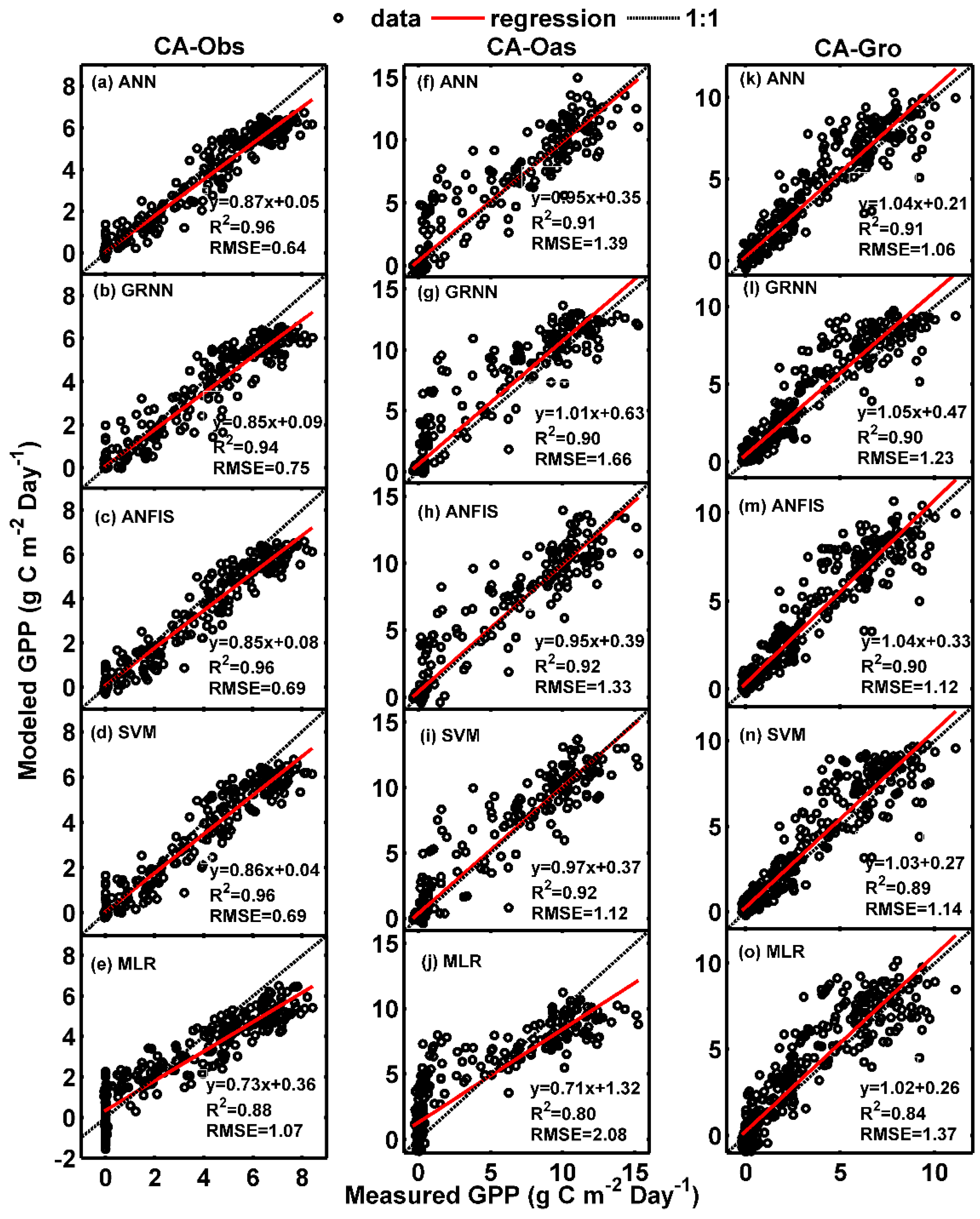
Figure 2.
Eddy covariance measured and model simulated daily gross primary productivity (GPP) in the whole period in the three boreal forest stands. (a) For CA-Obs stand using ANN model; (b) for CA-Oas stand using ANFIS model; and (c) for CA-Gro stand using ANN model.
Figure 2.
Eddy covariance measured and model simulated daily gross primary productivity (GPP) in the whole period in the three boreal forest stands. (a) For CA-Obs stand using ANN model; (b) for CA-Oas stand using ANFIS model; and (c) for CA-Gro stand using ANN model.
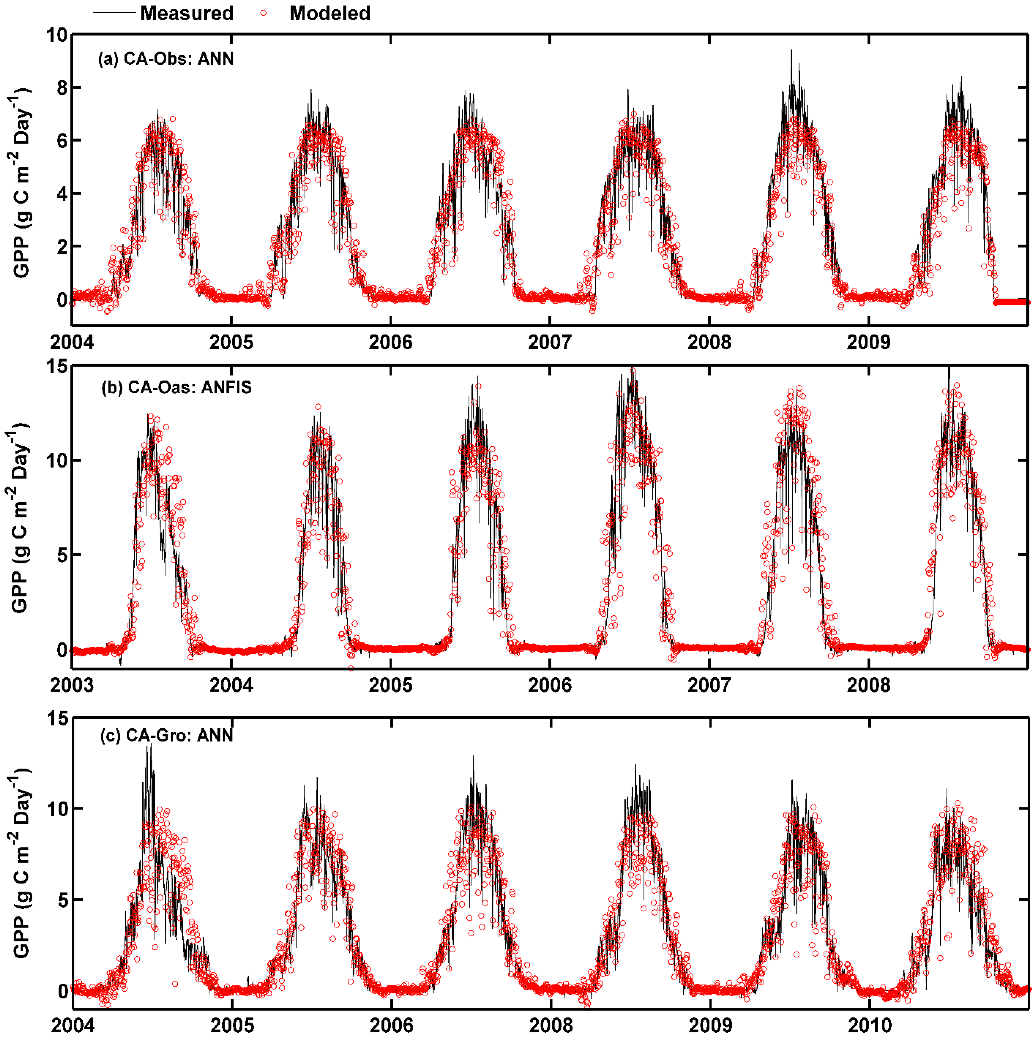
Figure 3.
Comparisons of measured and simulated daily ecosystem respiration (R) in the testing period in the three boreal forest stands. (a–e) For CA-Obs stand; (f–j) for CA-Oas stand; and (k–o) for CA-Gro stand.
Figure 3.
Comparisons of measured and simulated daily ecosystem respiration (R) in the testing period in the three boreal forest stands. (a–e) For CA-Obs stand; (f–j) for CA-Oas stand; and (k–o) for CA-Gro stand.

Figure 4.
Eddy covariance measured and model simulated daily ecosystem respiration (R) in the whole period in the three boreal forest stands. (a) For CA-Obs stand using ANN model; (b) for CA-Oas stand using ANFIS model; and (c) for CA-Gro stand using GRNN model.
Figure 4.
Eddy covariance measured and model simulated daily ecosystem respiration (R) in the whole period in the three boreal forest stands. (a) For CA-Obs stand using ANN model; (b) for CA-Oas stand using ANFIS model; and (c) for CA-Gro stand using GRNN model.

Figure 5.
Comparisons of measured and simulated daily net ecosystem exchange (NEE) in the testing period in the three boreal forest stands. (a–e) For CA-Obs stand; (f–j) for CA-Oas stand; and (k–o) for CA-Gro stand.
Figure 5.
Comparisons of measured and simulated daily net ecosystem exchange (NEE) in the testing period in the three boreal forest stands. (a–e) For CA-Obs stand; (f–j) for CA-Oas stand; and (k–o) for CA-Gro stand.

Figure 6.
Eddy covariance measured and model simulated daily net ecosystem exchange (NEE) in the whole period in the three boreal forest stands. (a) For CA-Obs stand using ANN model; (b) for CA-Oas stand using ANFIS model; and (c) for CA-Gro stand using GRNN model.
Figure 6.
Eddy covariance measured and model simulated daily net ecosystem exchange (NEE) in the whole period in the three boreal forest stands. (a) For CA-Obs stand using ANN model; (b) for CA-Oas stand using ANFIS model; and (c) for CA-Gro stand using GRNN model.

Figure 7.
Eddy covariance measured and ANFIS predicted hourly net ecosystem exchange (NEE) in the testing period. (a–c) Daily course of hourly NEE for 7 days during the mid-growing season at the three sites; and (d–f) Scatter plot of hourly NEE both in the daytime and nighttime datasets at each site.


Table 1.
Site characteristics used in this study. The mean annual temperature (MAT, °C) and total annual precipitation (TAP, mm year−1) are for the time period (Period). Vegetation types are deciduous broadleaf forest (DBF), evergreen needle-leaf forest (ENF) and mixed forest (MF).
Table 1.
Site characteristics used in this study. The mean annual temperature (MAT, °C) and total annual precipitation (TAP, mm year−1) are for the time period (Period). Vegetation types are deciduous broadleaf forest (DBF), evergreen needle-leaf forest (ENF) and mixed forest (MF).
| Site | Latitude | Longitude | Elevation | MAT | TAP | Vegetation | Period | Reference |
|---|---|---|---|---|---|---|---|---|
| CA-Oas | 53.63 | −106.20 | 601 | 1.82 | 343 | DBF | 2003–2008 | Griffis, et al. [35] |
| CA-Obs | 53.99 | −105.12 | 629 | 1.00 | 373 | ENF | 2004–2009 | Krishnan, et al. [36] |
| CA-Gro | 48.22 | −82.16 | 341 | 3.29 | 784 | MF | 2004–2006, 2008–2010 | McCaughey, et al. [37] |
Table 2.
Daily statistical parameters of flux tower measured environmental variables including air temperature (Ta, °C), net radiation (Rn, mol m−2), relative humidity (Rh, %), soil temperature (Ts, °C), gross primary productivity (GPP, g C m−2 day−1), ecosystem respiration (R, g C m−2 day−1) and net ecosystem exchange (NEE, g C m−2 day−1) during the whole period in all three stands.
| Stand | Variable | Xmean | Xmax | Xmin | Xsd | Xku | Xsk | CC1 | CC2 | CC3 |
|---|---|---|---|---|---|---|---|---|---|---|
| CA-Oas | Ta | 1.82 | 26.46 | −35.04 | 13.02 | 2.22 | −0.40 | 0.70 | 0.82 | −0.50 |
| Rn | 5.19 | 18.94 | −4.67 | 5.66 | 2.02 | 0.45 | 0.69 | 0.68 | −0.60 | |
| Rh | 69.88 | 98.78 | 21.83 | 16.15 | 2.62 | −0.52 | −0.18 | −0.21 | 0.13 | |
| Ts | 4.73 | 17.31 | −5.81 | 5.81 | 1.69 | 0.30 | 0.83 | 0.93 | −0.64 | |
| GPP | 2.87 | 15.99 | −0.84 | 4.29 | 2.83 | 1.17 | 1.00 | 0.91 | −0.94 | |
| R | 2.25 | 8.69 | −1.17 | 2.11 | 2.34 | 0.81 | 0.91 | 1.00 | −0.70 | |
| NEE | −0.62 | 4.34 | −10.41 | 2.55 | 3.69 | −1.29 | −0.94 | −0.70 | 1.00 | |
| CA-Obs | Ta | 1.00 | 26.37 | −35.31 | 13.15 | 2.15 | −0.34 | 0.83 | 0.81 | −0.58 |
| Rn | 6.71 | 21.90 | −4.28 | 6.17 | 2.05 | 0.48 | 0.72 | 0.56 | −0.71 | |
| Rh | 72.35 | 100.00 | 24.56 | 16.69 | 2.46 | −0.43 | −0.31 | −0.16 | 0.42 | |
| Ts | 3.19 | 15.41 | −9.18 | 4.99 | 1.99 | 0.58 | 0.87 | 0.94 | −0.48 | |
| GPP | 2.23 | 9.41 | −0.15 | 2.56 | 1.96 | 0.68 | 1.00 | 0.90 | −0.80 | |
| R | 1.70 | 7.28 | −0.26 | 1.73 | 2.66 | 0.97 | 0.90 | 1.00 | −0.47 | |
| NEE | −0.53 | 3.90 | −5.20 | 1.24 | 3.03 | −0.84 | −0.80 | −0.47 | 1.00 | |
| CA-Gro | Ta | 3.29 | 27.83 | −31.66 | 12.35 | 2.26 | −0.36 | 0.78 | 0.82 | −0.46 |
| Rn | 6.60 | 21.97 | −3.42 | 5.75 | 2.13 | 0.51 | 0.69 | 0.58 | −0.64 | |
| Rh | 74.98 | 98.93 | 21.54 | 15.47 | 3.27 | −0.78 | −0.25 | −0.18 | 0.27 | |
| Ts | 5.56 | 17.68 | −1.21 | 5.45 | 1.65 | 0.45 | 0.87 | 0.94 | −0.48 | |
| GPP | 2.88 | 13.59 | −0.45 | 3.38 | 2.70 | 0.98 | 1.00 | 0.92 | −0.80 | |
| R | 2.59 | 10.62 | −0.21 | 2.31 | 2.66 | 0.90 | 0.92 | 1.00 | −0.50 | |
| NEE | −0.29 | 4.27 | −8.51 | 1.56 | 5.64 | −1.42 | −0.80 | −0.50 | 1.00 |
Note: Xmean, Xmax, Xmin, Xsd, Xku and Xsk refer to the mean, maximum, minimum, standard deviation, kurtosis and skewness of each variable, respectively; CC1, CC2 and CC3 refer to the correlation coefficient between each variable and GPP, R and NEE, respectively.
Table 3.
The input combinations for different methods with environmental variables including air temperature (Ta, °C), net radiation (Rn, mol m−2), relative humidity (Rh, %), soil temperature (Ts, °C).
Table 3.
The input combinations for different methods with environmental variables including air temperature (Ta, °C), net radiation (Rn, mol m−2), relative humidity (Rh, %), soil temperature (Ts, °C).
| Models | Input Combinations | ||||
|---|---|---|---|---|---|
| ANN | GRNN | ANFIS | SVM | MLR | |
| ANN1 | GRNN1 | ANFIS1 | SVM1 | MLR1 | Ta |
| ANN2 | GRNN2 | ANFIS2 | SVM2 | MLR2 | Rn |
| ANN3 | GRNN3 | ANFIS3 | SVM3 | MLR3 | Rh |
| ANN4 | GRNN4 | ANFIS4 | SVM4 | MLR4 | Ts |
| ANN5 | GRNN5 | ANFIS5 | SVM5 | MLR5 | Ta, Rn |
| ANN6 | GRNN6 | ANFIS6 | SVM6 | MLR6 | Ta, Rn, Rh |
| ANN7 | GRNN7 | ANFIS7 | SVM7 | MLR7 | Ta, Rn, Rh, Ts |
Table 4.
Comparisons of machine learning models with different input combinations in the testing period for gross primary productivity (GPP, g C m−2 day−1) in the three boreal forest stands.
Table 4.
Comparisons of machine learning models with different input combinations in the testing period for gross primary productivity (GPP, g C m−2 day−1) in the three boreal forest stands.
| Model | CA-Obs | CA-Oas | CA-Gro | |||||||||
|---|---|---|---|---|---|---|---|---|---|---|---|---|
| R2 | NSE | Bias | RMSE | R2 | NSE | Bias | RMSE | R2 | NSE | Bias | RMSE | |
| ANN1 | 0.880 | 0.854 | −0.358 | 1.046 | 0.753 | 0.742 | −0.243 | 2.279 | 0.736 | 0.682 | 0.573 | 1.705 |
| ANN2 | 0.482 | 0.472 | 0.003 | 1.989 | 0.428 | 0.420 | 0.203 | 3.417 | 0.554 | 0.529 | 0.395 | 2.076 |
| ANN3 | 0.001 | −0.088 | 0.311 | 2.854 | 0.062 | 0.062 | 0.022 | 4.347 | 0.110 | 0.072 | 0.483 | 2.914 |
| ANN4 | 0.811 | 0.788 | −0.305 | 1.259 | 0.831 | 0.830 | 0.118 | 1.848 | 0.795 | 0.778 | 0.340 | 1.425 |
| ANN5 | 0.903 | 0.883 | −0.273 | 0.937 | 0.808 | 0.806 | −0.069 | 1.975 | 0.804 | 0.763 | 0.488 | 1.473 |
| ANN6 | 0.932 | 0.917 | −0.317 | 0.789 | 0.871 | 0.870 | −0.087 | 1.618 | 0.861 | 0.825 | 0.430 | 1.267 |
| ANN7 | 0.963 | 0.944 | −0.253 | 0.645 | 0.909 | 0.905 | 0.211 | 1.386 | 0.907 | 0.877 | 0.319 | 1.060 |
| GRNN1 | 0.876 | 0.825 | −0.488 | 1.145 | 0.752 | 0.720 | −0.524 | 2.377 | 0.734 | 0.699 | 0.486 | 1.660 |
| GRNN2 | 0.485 | 0.470 | 0.056 | 1.992 | 0.434 | 0.428 | 0.261 | 3.395 | 0.564 | 0.551 | 0.325 | 2.027 |
| GRNN3 | 0.000 | −0.108 | 0.367 | 2.881 | 0.063 | 0.058 | 0.082 | 4.357 | 0.125 | 0.090 | 0.527 | 2.886 |
| GRNN4 | 0.794 | 0.770 | −0.311 | 1.311 | 0.841 | 0.822 | −0.359 | 1.894 | 0.802 | 0.787 | 0.270 | 1.396 |
| GRNN5 | 0.904 | 0.882 | −0.282 | 0.941 | 0.786 | 0.786 | 0.050 | 2.078 | 0.795 | 0.733 | 0.598 | 1.562 |
| GRNN6 | 0.926 | 0.886 | −0.402 | 0.924 | 0.870 | 0.864 | −0.105 | 1.652 | 0.838 | 0.803 | 0.465 | 1.341 |
| GRNN7 | 0.944 | 0.925 | −0.259 | 0.747 | 0.900 | 0.864 | 0.667 | 1.655 | 0.899 | 0.834 | 0.603 | 1.234 |
| ANFIS1 | 0.882 | 0.856 | −0.353 | 1.037 | 0.750 | 0.741 | −0.222 | 2.286 | 0.736 | 0.695 | 0.504 | 1.669 |
| ANFIS2 | 0.474 | 0.459 | 0.087 | 2.013 | 0.414 | 0.402 | 0.266 | 3.470 | 0.565 | 0.549 | 0.354 | 2.031 |
| ANFIS3 | 0.000 | −0.124 | 0.440 | 2.901 | 0.063 | 0.062 | −0.061 | 4.347 | 0.127 | 0.088 | 0.550 | 2.889 |
| ANFIS4 | 0.785 | 0.764 | −0.314 | 1.329 | 0.806 | 0.806 | 0.077 | 1.977 | 0.804 | 0.780 | 0.294 | 1.420 |
| ANFIS5 | 0.902 | 0.883 | −0.309 | 0.938 | 0.790 | 0.790 | −0.033 | 2.058 | 0.797 | 0.749 | 0.526 | 1.515 |
| ANFIS6 | 0.938 | 0.921 | −0.302 | 0.771 | 0.886 | 0.884 | −0.135 | 1.529 | 0.866 | 0.823 | 0.485 | 1.271 |
| ANFIS7 | 0.960 | 0.936 | −0.271 | 0.690 | 0.917 | 0.913 | 0.249 | 1.326 | 0.904 | 0.863 | 0.438 | 1.120 |
| SVM1 | 0.876 | 0.851 | −0.354 | 1.056 | 0.754 | 0.745 | −0.295 | 2.268 | 0.732 | 0.698 | 0.397 | 1.662 |
| SVM2 | 0.501 | 0.498 | 0.136 | 1.939 | 0.392 | 0.304 | 0.334 | 3.744 | 0.564 | 0.545 | 0.188 | 2.041 |
| SVM3 | 0.001 | −0.362 | 0.116 | 3.193 | 0.035 | −0.350 | −2.735 | 5.215 | 0.090 | −0.012 | −0.530 | 3.043 |
| SVM4 | 0.758 | 0.725 | −0.498 | 1.434 | 0.868 | 0.867 | −0.007 | 1.638 | 0.802 | 0.780 | 0.185 | 1.420 |
| SVM5 | 0.902 | 0.886 | −0.274 | 0.924 | 0.796 | 0.796 | 0.048 | 2.029 | 0.800 | 0.755 | 0.483 | 1.497 |
| SVM6 | 0.932 | 0.919 | −0.237 | 0.781 | 0.881 | 0.881 | −0.059 | 1.547 | 0.865 | 0.813 | 0.490 | 1.307 |
| SVM7 | 0.956 | 0.936 | −0.281 | 0.695 | 0.916 | 0.910 | 0.276 | 1.350 | 0.894 | 0.859 | 0.359 | 1.136 |
| MLR1 | 0.758 | 0.707 | −0.586 | 1.480 | 0.510 | 0.498 | −0.490 | 3.177 | 0.615 | 0.568 | 0.637 | 1.988 |
| MLR2 | 0.465 | 0.453 | 0.040 | 2.024 | 0.408 | 0.397 | 0.292 | 3.482 | 0.556 | 0.539 | 0.375 | 2.054 |
| MLR3 | 0.000 | −0.076 | 0.220 | 2.837 | 0.019 | 0.018 | −0.124 | 4.443 | 0.033 | −0.029 | 0.499 | 3.067 |
| MLR4 | 0.778 | 0.746 | −0.350 | 1.379 | 0.752 | 0.738 | 0.108 | 2.297 | 0.766 | 0.723 | 0.351 | 1.591 |
| MLR5 | 0.759 | 0.731 | −0.387 | 1.419 | 0.542 | 0.539 | −0.065 | 3.044 | 0.699 | 0.654 | 0.583 | 1.779 |
| MLR6 | 0.786 | 0.744 | −0.551 | 1.384 | 0.604 | 0.601 | −0.187 | 2.832 | 0.738 | 0.702 | 0.517 | 1.650 |
| MLR7 | 0.882 | 0.846 | −0.262 | 1.074 | 0.805 | 0.785 | 0.430 | 2.081 | 0.843 | 0.793 | 0.318 | 1.375 |
Note: Bold numbers show the best performance among the models with different input combinations for each method and stand.
Table 5.
Comparisons of different models in the three stands for gross primary productivity (GPP, g C m−2 day−1), ecosystem respiration (R, g C m−2 day−1) and net ecosystem exchange (NEE, g C m−2 day−1) in the testing period.
Table 5.
Comparisons of different models in the three stands for gross primary productivity (GPP, g C m−2 day−1), ecosystem respiration (R, g C m−2 day−1) and net ecosystem exchange (NEE, g C m−2 day−1) in the testing period.
| Model | GPP | R | NEE | |||||||||
|---|---|---|---|---|---|---|---|---|---|---|---|---|
| R2 | NSE | Bias | RMSE | R2 | NSE | Bias | RMSE | R2 | NSE | Bias | RMSE | |
| ANN | 0.926 | 0.909 | 0.092 | 1.030 | 0.944 | 0.818 | 0.236 | 0.717 | 0.789 | 0.754 | 0.160 | 0.889 |
| GRNN | 0.914 | 0.874 | 0.337 | 1.212 | 0.936 | 0.887 | 0.148 | 0.624 | 0.770 | 0.731 | −0.017 | 0.950 |
| ANFIS | 0.927 | 0.904 | 0.138 | 1.045 | 0.944 | 0.816 | 0.243 | 0.725 | 0.785 | 0.751 | 0.132 | 0.889 |
| SVM | 0.922 | 0.901 | 0.118 | 1.060 | 0.941 | 0.812 | 0.260 | 0.737 | 0.779 | 0.738 | 0.173 | 0.914 |
| MLR | 0.843 | 0.808 | 0.162 | 1.510 | 0.915 | 0.799 | 0.256 | 0.807 | 0.569 | 0.523 | 0.094 | 1.258 |
Table 6.
Comparisons of different stands using all the five models for gross primary productivity (GPP, g C m−2 day−1), ecosystem respiration (R, g C m−2 day−1) and net ecosystem exchange (NEE, g C m−2 day−1) in the testing period.
Table 6.
Comparisons of different stands using all the five models for gross primary productivity (GPP, g C m−2 day−1), ecosystem respiration (R, g C m−2 day−1) and net ecosystem exchange (NEE, g C m−2 day−1) in the testing period.
| Stand | GPP | R | NEE | |||||||||
|---|---|---|---|---|---|---|---|---|---|---|---|---|
| R2 | NSE | Bias | RMSE | R2 | NSE | Bias | RMSE | R2 | NSE | Bias | RMSE | |
| CA-Obs | 0.941 | 0.918 | −0.265 | 0.770 | 0.937 | 0.925 | −0.027 | 0.496 | 0.764 | 0.714 | 0.208 | 0.701 |
| CA-Oas | 0.889 | 0.875 | 0.367 | 1.56 | 0.919 | 0.917 | 0.070 | 0.622 | 0.769 | 0.756 | −0.188 | 1.272 |
| CA-Gro | 0.889 | 0.845 | 0.407 | 1.185 | 0.952 | 0.637 | 0.643 | 1.047 | 0.682 | 0.628 | 0.305 | 0.966 |
Table 7.
Comparisons of machine learning models with different input combinations in the testing period for ecosystem respiration (R, g C m−2 day−1) in the three boreal forest stands.
Table 7.
Comparisons of machine learning models with different input combinations in the testing period for ecosystem respiration (R, g C m−2 day−1) in the three boreal forest stands.
| Model | CA-Obs | CA-Oas | CA-Gro | |||||||||
|---|---|---|---|---|---|---|---|---|---|---|---|---|
| R2 | NSE | Bias | RMSE | R2 | NSE | Bias | RMSE | R2 | NSE | Bias | RMSE | |
| ANN1 | 0.829 | 0.821 | −0.032 | 0.776 | 0.837 | 0.830 | −0.116 | 0.892 | 0.847 | 0.487 | 0.802 | 1.258 |
| ANN2 | 0.258 | 0.234 | 0.275 | 1.606 | 0.378 | 0.364 | 0.122 | 1.725 | 0.421 | 0.246 | 0.677 | 1.525 |
| ANN3 | 0.011 | −0.148 | 0.428 | 1.967 | 0.055 | 0.053 | 0.011 | 2.105 | 0.070 | −0.173 | 0.799 | 1.902 |
| ANN4 | 0.904 | 0.881 | 0.076 | 0.634 | 0.904 | 0.902 | 0.073 | 0.675 | 0.938 | 0.618 | 0.721 | 1.085 |
| ANN5 | 0.842 | 0.832 | −0.083 | 0.752 | 0.830 | 0.828 | −0.074 | 0.897 | 0.853 | 0.467 | 0.849 | 1.282 |
| ANN6 | 0.913 | 0.907 | 0.023 | 0.560 | 0.893 | 0.892 | −0.048 | 0.710 | 0.908 | 0.573 | 0.740 | 1.148 |
| ANN7 | 0.954 | 0.946 | −0.033 | 0.428 | 0.927 | 0.927 | 0.027 | 0.585 | 0.950 | 0.580 | 0.714 | 1.138 |
| GRNN1 | 0.827 | 0.807 | −0.081 | 0.807 | 0.822 | 0.821 | 0.007 | 0.914 | 0.852 | 0.414 | 0.952 | 1.345 |
| GRNN2 | 0.272 | 0.252 | 0.236 | 1.588 | 0.381 | 0.368 | 0.134 | 1.719 | 0.418 | 0.284 | 0.604 | 1.487 |
| GRNN3 | 0.012 | −0.141 | 0.394 | 1.961 | 0.047 | 0.032 | 0.267 | 2.128 | 0.080 | −0.166 | 0.848 | 1.897 |
| GRNN4 | 0.905 | 0.889 | −0.059 | 0.610 | 0.904 | 0.901 | 0.082 | 0.679 | 0.950 | 0.680 | 0.672 | 0.993 |
| GRNN5 | 0.837 | 0.816 | −0.101 | 0.788 | 0.828 | 0.812 | 0.249 | 0.937 | 0.848 | 0.532 | 0.794 | 1.202 |
| GRNN6 | 0.895 | 0.886 | −0.020 | 0.620 | 0.873 | 0.872 | 0.062 | 0.775 | 0.902 | 0.595 | 0.759 | 1.118 |
| GRNN7 | 0.941 | 0.929 | −0.037 | 0.488 | 0.914 | 0.914 | 0.032 | 0.635 | 0.954 | 0.818 | 0.448 | 0.749 |
| ANFIS1 | 0.828 | 0.821 | −0.029 | 0.776 | 0.834 | 0.830 | −0.091 | 0.890 | 0.849 | 0.500 | 0.804 | 1.242 |
| ANFIS2 | 0.243 | 0.219 | 0.280 | 1.622 | 0.381 | 0.364 | 0.170 | 1.725 | 0.422 | 0.251 | 0.676 | 1.520 |
| ANFIS3 | 0.014 | −0.176 | 0.426 | 1.991 | 0.050 | 0.049 | 0.013 | 2.109 | 0.082 | −0.135 | 0.775 | 1.872 |
| ANFIS4 | 0.904 | 0.894 | −0.010 | 0.596 | 0.913 | 0.910 | 0.081 | 0.650 | 0.947 | 0.621 | 0.671 | 1.081 |
| ANFIS5 | 0.846 | 0.840 | −0.050 | 0.735 | 0.839 | 0.839 | −0.035 | 0.868 | 0.853 | 0.479 | 0.837 | 1.268 |
| ANFIS6 | 0.912 | 0.906 | −0.007 | 0.563 | 0.903 | 0.901 | −0.093 | 0.682 | 0.910 | 0.532 | 0.788 | 1.201 |
| ANFIS7 | 0.947 | 0.935 | −0.019 | 0.468 | 0.930 | 0.930 | 0.040 | 0.574 | 0.954 | 0.584 | 0.709 | 1.132 |
| SVM1 | 0.826 | 0.818 | −0.062 | 0.783 | 0.837 | 0.835 | −0.098 | 0.878 | 0.851 | 0.546 | 0.743 | 1.183 |
| SVM2 | 0.248 | 0.244 | 0.062 | 1.596 | 0.380 | 0.333 | 0.104 | 1.766 | 0.426 | 0.235 | 0.514 | 1.536 |
| SVM3 | 0.025 | −0.253 | −0.143 | 2.055 | 0.049 | −0.101 | −0.773 | 2.269 | 0.072 | −0.095 | 0.091 | 1.838 |
| SVM4 | 0.907 | 0.898 | −0.049 | 0.588 | 0.912 | 0.908 | 0.116 | 0.654 | 0.945 | 0.646 | 0.645 | 1.045 |
| SVM5 | 0.843 | 0.832 | −0.108 | 0.752 | 0.840 | 0.838 | −0.077 | 0.869 | 0.855 | 0.534 | 0.766 | 1.199 |
| SVM6 | 0.910 | 0.901 | −0.052 | 0.577 | 0.899 | 0.895 | −0.107 | 0.699 | 0.916 | 0.516 | 0.803 | 1.222 |
| SVM7 | 0.947 | 0.935 | −0.017 | 0.469 | 0.925 | 0.923 | 0.088 | 0.601 | 0.951 | 0.579 | 0.709 | 1.140 |
| MLR1 | 0.697 | 0.686 | −0.182 | 1.028 | 0.659 | 0.647 | −0.208 | 1.285 | 0.734 | 0.435 | 0.874 | 1.321 |
| MLR2 | 0.242 | 0.227 | 0.221 | 1.613 | 0.377 | 0.356 | 0.196 | 1.736 | 0.418 | 0.252 | 0.665 | 1.520 |
| MLR3 | 0.026 | −0.110 | 0.282 | 1.933 | 0.026 | 0.025 | 0.008 | 2.135 | 0.011 | −0.224 | 0.732 | 1.944 |
| MLR4 | 0.877 | 0.868 | −0.041 | 0.667 | 0.898 | 0.885 | 0.127 | 0.733 | 0.945 | 0.629 | 0.660 | 1.070 |
| MLR5 | 0.684 | 0.677 | −0.153 | 1.043 | 0.654 | 0.647 | −0.081 | 1.284 | 0.742 | 0.442 | 0.861 | 1.312 |
| MLR6 | 0.734 | 0.702 | −0.316 | 1.002 | 0.700 | 0.691 | −0.133 | 1.202 | 0.792 | 0.522 | 0.810 | 1.215 |
| MLR7 | 0.893 | 0.882 | −0.031 | 0.629 | 0.902 | 0.891 | 0.163 | 0.715 | 0.951 | 0.625 | 0.636 | 1.076 |
Table 8.
Comparisons of machine learning models with different input combinations in the testing period for net ecosystem exchange (NEE, g C m−2 day−1) in the three boreal forest stands.
Table 8.
Comparisons of machine learning models with different input combinations in the testing period for net ecosystem exchange (NEE, g C m−2 day−1) in the three boreal forest stands.
| Model | CA-Obs | CA-Oas | CA-Gro | |||||||||
|---|---|---|---|---|---|---|---|---|---|---|---|---|
| R2 | NSE | Bias | RMSE | R2 | NSE | Bias | RMSE | R2 | NSE | Bias | RMSE | |
| ANN1 | 0.502 | 0.438 | 0.313 | 0.998 | 0.553 | 0.536 | 0.165 | 1.782 | 0.387 | 0.310 | 0.358 | 1.321 |
| ANN2 | 0.514 | 0.465 | 0.222 | 0.974 | 0.376 | 0.362 | −0.151 | 2.090 | 0.507 | 0.475 | 0.250 | 1.152 |
| ANN3 | 0.054 | 0.026 | −0.073 | 1.314 | 0.067 | 0.064 | 0.065 | 2.532 | 0.107 | 0.098 | 0.126 | 1.510 |
| ANN4 | 0.423 | 0.332 | 0.382 | 1.088 | 0.614 | 0.614 | 0.026 | 1.625 | 0.412 | 0.333 | 0.301 | 1.299 |
| ANN5 | 0.736 | 0.701 | 0.207 | 0.728 | 0.638 | 0.636 | 0.039 | 1.580 | 0.605 | 0.559 | 0.315 | 1.056 |
| ANN6 | 0.775 | 0.719 | 0.270 | 0.705 | 0.744 | 0.744 | 0.004 | 1.325 | 0.674 | 0.631 | 0.301 | 0.966 |
| ANN7 | 0.830 | 0.785 | 0.232 | 0.618 | 0.817 | 0.815 | −0.073 | 1.125 | 0.719 | 0.663 | 0.322 | 0.923 |
| GRNN1 | 0.515 | 0.433 | 0.330 | 1.003 | 0.558 | 0.538 | 0.134 | 1.779 | 0.402 | 0.346 | 0.276 | 1.286 |
| GRNN2 | 0.528 | 0.464 | 0.271 | 0.975 | 0.376 | 0.352 | −0.387 | 2.106 | 0.507 | 0.481 | 0.249 | 1.146 |
| GRNN3 | 0.050 | 0.035 | 0.124 | 1.309 | 0.073 | 0.066 | 0.034 | 2.529 | 0.107 | 0.067 | −0.311 | 1.537 |
| GRNN4 | 0.368 | 0.297 | 0.313 | 1.117 | 0.685 | 0.627 | −0.557 | 1.597 | 0.420 | 0.337 | 0.344 | 1.295 |
| GRNN5 | 0.739 | 0.685 | 0.235 | 0.748 | 0.637 | 0.606 | −0.344 | 1.642 | 0.614 | 0.274 | 0.927 | 1.355 |
| GRNN6 | 0.779 | 0.725 | 0.079 | 0.699 | 0.714 | 0.694 | −0.339 | 1.447 | 0.661 | 0.554 | 0.436 | 1.062 |
| GRNN7 | 0.805 | 0.766 | 0.055 | 0.644 | 0.787 | 0.755 | −0.353 | 1.294 | 0.718 | 0.672 | 0.246 | 0.911 |
| ANFIS1 | 0.510 | 0.438 | 0.327 | 0.998 | 0.535 | 0.525 | 0.147 | 1.803 | 0.396 | 0.335 | 0.304 | 1.296 |
| ANFIS2 | 0.531 | 0.482 | 0.193 | 0.959 | 0.354 | 0.345 | −0.106 | 2.117 | 0.510 | 0.468 | 0.304 | 1.160 |
| ANFIS3 | 0.052 | 0.038 | −0.008 | 1.307 | 0.071 | 0.066 | 0.067 | 2.529 | 0.129 | 0.109 | 0.223 | 1.501 |
| ANFIS4 | 0.338 | 0.281 | 0.297 | 1.130 | 0.694 | 0.692 | 0.026 | 1.453 | 0.433 | 0.336 | 0.377 | 1.296 |
| ANFIS5 | 0.732 | 0.678 | 0.240 | 0.756 | 0.640 | 0.639 | −0.028 | 1.572 | 0.609 | 0.565 | 0.304 | 1.049 |
| ANFIS6 | 0.804 | 0.739 | 0.281 | 0.681 | 0.761 | 0.759 | 0.032 | 1.285 | 0.683 | 0.628 | 0.322 | 0.970 |
| ANFIS7 | 0.808 | 0.758 | 0.264 | 0.655 | 0.830 | 0.824 | −0.158 | 1.097 | 0.716 | 0.670 | 0.289 | 0.914 |
| SVM1 | 0.490 | 0.449 | 0.262 | 0.988 | 0.552 | 0.539 | 0.184 | 1.776 | 0.424 | 0.348 | 0.336 | 1.284 |
| SVM2 | 0.539 | 0.482 | 0.253 | 0.958 | 0.315 | 0.241 | −0.289 | 2.279 | 0.493 | 0.413 | 0.388 | 1.218 |
| SVM3 | 0.031 | −0.063 | 0.137 | 1.373 | 0.012 | −0.192 | 1.178 | 2.857 | 0.078 | −0.058 | 0.583 | 1.636 |
| SVM4 | 0.244 | 0.133 | 0.432 | 1.240 | 0.708 | 0.701 | 0.052 | 1.430 | 0.446 | 0.325 | 0.468 | 1.307 |
| SVM5 | 0.737 | 0.697 | 0.202 | 0.733 | 0.642 | 0.640 | −0.051 | 1.569 | 0.630 | 0.564 | 0.318 | 1.050 |
| SVM6 | 0.795 | 0.755 | 0.212 | 0.659 | 0.737 | 0.737 | 0.023 | 1.343 | 0.666 | 0.597 | 0.355 | 1.010 |
| SVM7 | 0.818 | 0.768 | 0.258 | 0.641 | 0.811 | 0.809 | −0.089 | 1.142 | 0.707 | 0.636 | 0.351 | 0.959 |
| MLR1 | 0.408 | 0.305 | 0.404 | 1.109 | 0.307 | 0.294 | 0.282 | 2.196 | 0.298 | 0.254 | 0.237 | 1.372 |
| MLR2 | 0.524 | 0.467 | 0.182 | 0.972 | 0.345 | 0.342 | −0.096 | 2.120 | 0.496 | 0.455 | 0.289 | 1.173 |
| MLR3 | 0.057 | 0.049 | 0.062 | 1.298 | 0.011 | 0.008 | 0.132 | 2.603 | 0.052 | 0.025 | 0.233 | 1.569 |
| MLR4 | 0.273 | 0.201 | 0.310 | 1.190 | 0.495 | 0.481 | 0.018 | 1.883 | 0.349 | 0.292 | 0.309 | 1.337 |
| MLR5 | 0.557 | 0.491 | 0.234 | 0.949 | 0.379 | 0.378 | −0.016 | 2.060 | 0.503 | 0.464 | 0.278 | 1.163 |
| MLR6 | 0.557 | 0.492 | 0.235 | 0.949 | 0.443 | 0.443 | 0.054 | 1.951 | 0.518 | 0.475 | 0.293 | 1.151 |
| MLR7 | 0.560 | 0.493 | 0.231 | 0.948 | 0.598 | 0.576 | −0.267 | 1.703 | 0.548 | 0.499 | 0.319 | 1.124 |
Table 9.
Comparisons of different models with four input variables for predicting hourly gross primary productivity (GPP, g C m−2 hour−1), ecosystem respiration (R, g C m−2 hour−1) and net ecosystem exchange (NEE, g C m−2 hour−1) in the testing period in the three boreal forest stands.
Table 9.
Comparisons of different models with four input variables for predicting hourly gross primary productivity (GPP, g C m−2 hour−1), ecosystem respiration (R, g C m−2 hour−1) and net ecosystem exchange (NEE, g C m−2 hour−1) in the testing period in the three boreal forest stands.
| Site | Model | GPP | R | NEE | |||||||||
|---|---|---|---|---|---|---|---|---|---|---|---|---|---|
| R2 | NSE | Bias | RMSE | R2 | NSE | Bias | RMSE | R2 | NSE | Bias | RMSE | ||
| CA-Obs | ANN | 0.932 | 0.910 | −0.015 | 0.056 | 0.843 | 0.832 | 0.001 | 0.036 | 0.850 | 0.821 | 0.013 | 0.060 |
| GRNN | 0.924 | 0.905 | −0.009 | 0.057 | 0.827 | 0.577 | −0.040 | 0.057 | 0.819 | 0.789 | 0.015 | 0.065 | |
| ANFIS | 0.914 | 0.890 | −0.016 | 0.061 | 0.838 | 0.823 | −0.002 | 0.037 | 0.844 | 0.811 | 0.013 | 0.061 | |
| SVM | 0.925 | 0.904 | −0.015 | 0.057 | 0.833 | 0.826 | 0.001 | 0.037 | 0.842 | 0.814 | 0.011 | 0.061 | |
| MLR | 0.690 | 0.671 | −0.008 | 0.106 | 0.723 | 0.714 | 0.001 | 0.047 | 0.544 | 0.526 | 0.008 | 0.097 | |
| CA-Oas | ANN | 0.893 | 0.893 | 0.006 | 0.094 | 0.767 | 0.766 | 0.001 | 0.049 | 0.834 | 0.832 | −0.008 | 0.096 |
| GRNN | 0.885 | 0.877 | −0.024 | 0.101 | 0.755 | 0.729 | −0.016 | 0.053 | 0.828 | 0.828 | 0.001 | 0.097 | |
| ANFIS | 0.886 | 0.886 | 0.005 | 0.097 | 0.769 | 0.768 | 0.001 | 0.049 | 0.819 | 0.819 | −0.004 | 0.100 | |
| SVM | 0.893 | 0.892 | 0.006 | 0.095 | 0.766 | 0.765 | 0.002 | 0.049 | 0.834 | 0.832 | −0.008 | 0.096 | |
| MLR | 0.606 | 0.601 | 0.017 | 0.182 | 0.737 | 0.730 | 0.005 | 0.053 | 0.460 | 0.457 | −0.012 | 0.173 | |
| CA-Gro | ANN | 0.859 | 0.844 | 0.016 | 0.088 | 0.887 | 0.563 | 0.030 | 0.051 | 0.810 | 0.803 | 0.013 | 0.087 |
| GRNN | 0.850 | 0.728 | 0.077 | 0.116 | 0.884 | 0.399 | -0.085 | 0.091 | 0.800 | 0.715 | 0.057 | 0.104 | |
| ANFIS | 0.846 | 0.829 | 0.019 | 0.092 | 0.889 | 0.587 | 0.029 | 0.049 | 0.794 | 0.789 | 0.010 | 0.090 | |
| SVM | 0.853 | 0.838 | 0.015 | 0.090 | 0.883 | 0.572 | 0.028 | 0.050 | 0.803 | 0.796 | 0.013 | 0.088 | |
| MLR | 0.634 | 0.621 | 0.014 | 0.137 | 0.884 | 0.591 | 0.028 | 0.049 | 0.531 | 0.526 | 0.014 | 0.134 | |
Table 10.
Comparisons of different models with four input variables for predicting hourly net ecosystem exchange (NEE, g C m−2 hour−1) in the testing period for daytime and nighttime datasets in the three boreal forest stands.
Table 10.
Comparisons of different models with four input variables for predicting hourly net ecosystem exchange (NEE, g C m−2 hour−1) in the testing period for daytime and nighttime datasets in the three boreal forest stands.
| Model | Dataset | CA-Obs | CA-Oas | CA-Gro | |||||||||
|---|---|---|---|---|---|---|---|---|---|---|---|---|---|
| R2 | NSE | Bias | RMSE | R2 | NSE | Bias | RMSE | R2 | NSE | Bias | RMSE | ||
| ANN | Daytime | 0.847 | 0.809 | 0.023 | 0.076 | 0.822 | 0.820 | −0.010 | 0.121 | 0.765 | 0.761 | 0.012 | 0.111 |
| Nighttime | 0.566 | 0.533 | 0.004 | 0.041 | 0.590 | 0.580 | −0.005 | 0.052 | 0.799 | 0.674 | 0.015 | 0.041 | |
| GRNN | Daytime | 0.824 | 0.784 | 0.024 | 0.081 | 0.814 | 0.814 | 0.003 | 0.123 | 0.750 | 0.677 | 0.061 | 0.129 |
| Nighttime | 0.400 | 0.385 | 0.006 | 0.047 | 0.601 | 0.589 | −0.002 | 0.051 | 0.803 | 0.251 | 0.052 | 0.062 | |
| ANFIS | Daytime | 0.841 | 0.799 | 0.025 | 0.078 | 0.814 | 0.814 | −0.005 | 0.123 | 0.753 | 0.751 | 0.008 | 0.113 |
| Nighttime | 0.544 | 0.511 | 0.003 | 0.042 | 0.419 | 0.414 | −0.003 | 0.061 | 0.684 | 0.568 | 0.012 | 0.047 | |
| SVM | Daytime | 0.844 | 0.807 | 0.022 | 0.077 | 0.822 | 0.820 | −0.007 | 0.121 | 0.757 | 0.753 | 0.012 | 0.113 |
| Nighttime | 0.496 | 0.476 | 0.002 | 0.043 | 0.582 | 0.569 | −0.008 | 0.053 | 0.784 | 0.645 | 0.015 | 0.043 | |
| MLR | Daytime | 0.483 | 0.456 | 0.021 | 0.129 | 0.453 | 0.443 | −0.014 | 0.213 | 0.457 | 0.451 | 0.017 | 0.169 |
| Nighttime | 0.073 | 0.061 | −0.003 | 0.058 | 0.121 | 0.176 | −0.010 | 0.107 | 0.012 | 0.105 | 0.010 | 0.075 | |
© 2018 by the authors. Licensee MDPI, Basel, Switzerland. This article is an open access article distributed under the terms and conditions of the Creative Commons Attribution (CC BY) license (http://creativecommons.org/licenses/by/4.0/).
Share and Cite
MDPI and ACS Style
Dou, X.; Yang, Y.; Luo, J. Estimating Forest Carbon Fluxes Using Machine Learning Techniques Based on Eddy Covariance Measurements. Sustainability 2018, 10, 203. https://doi.org/10.3390/su10010203
AMA Style
Dou X, Yang Y, Luo J. Estimating Forest Carbon Fluxes Using Machine Learning Techniques Based on Eddy Covariance Measurements. Sustainability. 2018; 10(1):203. https://doi.org/10.3390/su10010203
Chicago/Turabian StyleDou, Xianming, Yongguo Yang, and Jinhui Luo. 2018. "Estimating Forest Carbon Fluxes Using Machine Learning Techniques Based on Eddy Covariance Measurements" Sustainability 10, no. 1: 203. https://doi.org/10.3390/su10010203
Note that from the first issue of 2016, this journal uses article numbers instead of page numbers. See further details here.