A Study on the Sustainable Performance of the Steel Industry in Korea Based on SBM-DEA


1
Global E-Governance Program, Inha University, Inharo100, Nam-gu, Incheon 402-751, Korea
2
Institute of Resource, Environment and Sustainable Development (IRESD), Jinan University, Guangzhou 510632, China
*
Authors to whom correspondence should be addressed.
Sustainability 2018, 10(1), 173; https://doi.org/10.3390/su10010173
Submission received: 1 November 2017
/
Revised: 21 December 2017
/
Accepted: 8 January 2018
/
Published: 12 January 2018
(This article belongs to the Special Issue Regional Cooperation for the Sustainable Development and Management in Northeast Asia)
Abstract
:Since South Korea has implemented its emissions trading scheme (ETS) in 2015, several studies have explored the sustainable performance of ETS in terms of production efficiency. However, few studies focused on Korean company-level data in their model. Thus, this study focuses on data from firms in the steel industry, which is a representative greenhouse gas emitter. Based on the slack-based measure (SBM) approach, we find the following implications: First, this paper evaluates both environment energy efficiency (EEE) and traditional energy efficiency and discovers that the efficiency value, in general, is overestimated, when greenhouse gas emissions are ignored. EEE still shows a decreasing efficiency value over time, implying that strong regulation is needed to increase efficiency. Second, this paper provides the return to scale status of decision-making units in the steel industry, through decomposing EEE. Results show that many steel firms are in the state of increasing returns to scale, so they can enhance their efficiency by increasing their scale. Finally, this paper provides benchmark information with which an inefficient firm can enhance its performance.
1. Introduction
South Korea (hereafter “Korea”) has promoted its ambitious green growth optimal path control up to 2030, since it hosted the 2009 G20 summit in Seoul. As one of the core solutions to meet this challenge, Korea initiated the emissions trading scheme (ETS) in 2015. To accomplish its ambitious challenge, the government has made great efforts to decrease greenhouse gases (GHG) based on a selective concentration on the heavier emitters across all the major industries. Unfortunately, there are many debates on the “pros” and “cons” regarding this ETS policy, especially in its sustainable performance to reduce GHG levels, while maintaining Korea’s competitiveness in international trade. Prior to the Korean ETS, EU has similar problems. According to Martin, Muuls and Wagner (2016), the allocation of carbon emission allowances for free in the initial stages of the EU-ETS resulted in firms with high carbon emissions actually benefitting from the EU-ETS [1]. Oestreich and Tsiakas also found that this kind of carbon premium, coming from transition trial and error on the inappropriate carbon market price, is shown for a specific period that commences about one year before the beginning of Phase I and disappears about one year into Phase II [2]. Based on this experience of the EU ETS, the Korean government should make this kind of trial and error on the carbon market price as short as possible [3]. In this perspective, the feasibility analysis of ETS policies is crucial for sustainable development in Korea as it just initiated its ETS.
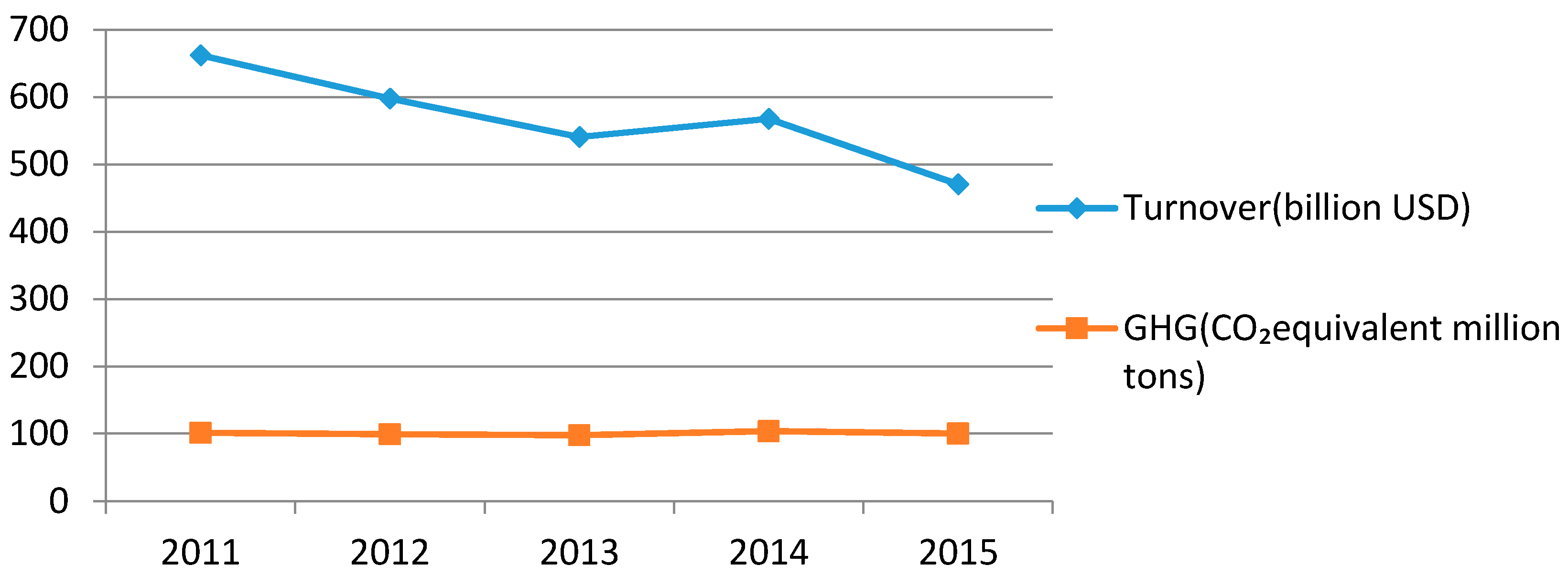
The steel industry is called the “rice of industry” due to its importance as a platform industry of the national economy. It is also true that without sustainable performance of the steel industry, it is impossible for heavy industries, such as the automotive, shipbuilding, and mechanical equipment industries, to be sustainable (see Appendix A). Thus, the steel industry is the platform industry because it is related to the sustainable performance of other industries as well. At the same time, the steel industry is also one of heaviest energy consumers. Its share of energy consumption among manufacturing industries in Korea is 27% [4]. Thus, the volume of GHG produced by the steel industry is overwhelming compared to that by other industries. Hence, the amount of carbon emissions allocation for the steel industry among industries covered by the Korean ETS is also large. Therefore, it is essential to manage the steel industry so that it reduces its GHG emissions by up to 37% until 2030. However, in contrast to the fact that GHG emissions have been stable for five years, as shown in Table 1 and Figure 1, firms’ revenues have been decreasing (Based on the comments by a reviewer, we changed all the turnover volume at the constant dollar terms in 2011. Our current measure (nominal $US) could be affected by price changes, which are unrelated to efficiency measures as a reviewer commented. We checked the possible change in the trend due to the exchange rate fluctuation, and determined there is no significant change. We found there is temporal upturn in 2014 due to the exchange rate fluctuation, but it was not significant to change the empirical results). Therefore, it is important to examine whether this decreasing trend in revenues may or may not stem from the newly-introduced environmental regulation in the steel industry. In addition, from this analysis, we could speculate about the industrial characteristics of ETS-covered steel firms, especially regarding returns to scale, and suggest the optimal way to increase each firm’s performance compared to the benchmark case. This is the basic motivation for this study.
There are two widely used methods for measuring production efficiency: stochastic frontier analysis (SFA), based on a parametric approach, and data envelopment analysis (DEA), based on a nonparametric relative scale. In general, the SFA model is used to calculate shadow price. Wang et al. [5] estimate shadow prices of steel enterprises in China. Che [6] estimates CO2 shadow prices in China’s iron and steel industry at the regional level, from 2006 to 2012. The characteristics of SFA are based on the theoretic form of the production function. Due to this functional constraint, there is also the limitation that an incorrect functional form may lead to incorrect results [7].
Meanwhile, the DEA model proposed by Charnes et al. [8] has some advantageous characteristics. First, it derives sole relative efficiency, which makes it suitable to be adopted in a complex industrial environment. Second, the DEA approach does not require the imposition of a functional form on the underlying environmental technology; it provides an easier and more flexible means of estimation [9]. Finally, for ineffective DMUs (decision making units), DEA can provide the corresponding improvement suggestions according to the projection theorem. Due to these advantages of DEA, there have been diverse papers that analyze the steel industry by adopting the DEA model. Zhang and Zhang [10] examined the technical efficiency of China’s iron and steel firms in the 1990s using the DEA approach. Yang et al. [11] also analyzed the Chinese regional iron steel industry through network bootstrapping DEA model and discovered a significant geographical difference across provinces. Wei et al. [12] analyzed the energy efficiency of the Chinese iron and steel industry by using DEA. Cho and Bae [13] measured the total factor productivity (TFP) changes in Northeast Asian countries’ steel industries and decomposed the TFP change into technical change and technical efficiency. Sheng and Song [14] used firm-level census data to calculate the TFP of firms in China’s iron and steel industry and examined its potential determinants over the period from 1998 to 2007.
With respect to the Korean steel industry, Lee and Kim [15] used a DEA model to analyze the steel industry. The results provided a comparison of efficiency between CCR, BCC, and each firm’s returns to scale (RTS). Ha and Choi [16] adopted DEA to evaluate the steel industry. Their study conducted a super efficiency test for efficient DMUs that show an efficiency of 1 and distinguished between them. In addition, this study also provided a benchmark result and suggested the implications for the Korean steel industry. However, these previous studies evaluating the performance of the Korean steel industry neglected to address the environmental impact of undesirable output, such as greenhouse gases. Almost all of them used desirable output only. Since the steel industry is a representative GHG-emitting industry, if undesirable output is ignored, the estimated efficiency value will be overestimated. To evaluate the unbiased sustainable performance, GHG emission should be incorporated into the model framework as undesirable output. Furthermore, previous studies did not take into consideration the effect of ETS, because this policy was launched in 2015. To overcome all these limitations, we examine unbiased production efficiency with undesirable output of GHG to determine whether ETS policies directly influence efficiency.
Meanwhile, a DEA model could be divided into two types of approaches: radial and non-radial models. A radial model is an approach adjusting input and undesirable output by the same proportion to the efficiency target. Thus, it may lack some information regarding the idle (or neglected) efficiency of the specific inputs or outputs involved in the production process [17]. Moreover, the radial efficiency approach neglects the slack variable, leading to biased estimation [18], and it has weak discriminating power for ranking and comparing decision making units (DMU). Due to these limitations, we introduce slacks-based measure (SBM)-DEA, which directly accounts for input and output slacks in the efficiency measurements, with the advantage of capturing the entire aspect of inefficiency. In the Energy and Environment (E and E) field, there have been diverse studies adopting an SBM model to explore efficiencies with undesirable output [10,18,19].
In addition, since SBM always assumes the non-radial approach, it can overcome the limitations of a radial model. We can determine the difference between radial and non-radial approaches in Figure 2. As shown in this figure, under the radial approach, DMU “c” should move to “a” on the efficiency frontier. To move point “a”, “ef” amount of energy input should be saved in this process, because the radial model is based on the proportional reduction and enlargement of variables. However, SBM deals directly with input excess (potential reduction) and output shortfall (potential expansion) of an observation, by using variables called slack variables. The SBM projects the observations to the furthest point on the efficient frontier, in the sense that the objective function is to be minimized by finding the maximum amounts of slacks. Under SBM, “c” could move to “b”, and this means that the value of the potential reduction in energy input could drop from “oe” to “od”. To examine this characteristic of SBM in our empirical study, we will also compare two results derived from a radial and non-radial model, respectively.
Therefore, the purpose of this paper is to suggest the following implications: First, we will examine the efficiencies of 20 ETS-covered Korean firms in the steel industry for five years (2011–2015). In fact, the Korean government inaugurated Korean ETS in 2015 and, thus, it might that be our empirical tests do not reflect well the policy effect on the firm’s performance. However, since the Korean government initiated its carbon targeting management system (TMS) in 2010, it is implied that the regulatory effect of ETS could be reflected well in our empirical tests. Nonetheless, the short-test period may not cover the full trials and errors in the initial stage.
Based on the result, we can find each firm’s efficiency status for five years and the efficiency change over time. In addition, we can check whether undesirable output causes a significant efficiency difference. Second, we will provide “returns to scale” for each DMU, and this will be helpful for each DMU when deciding the optimal path in their production. Third, we will arrange for benchmark information that each DMU can find in their concrete input-output structure to increase their efficiency.
Most of all, this paper aims to prove that the strong regulatory policies are much more important to shorten the trials and errors experienced in EU-ETs. Especially, under the strong regulatory regime, the firms shall more effectively find their role models as the benchmark to enhance their short-term environmental energy efficiency.
2. Methodology
In this section, the SBM model will be introduced in the first stage. The model shows how to estimate environmental energy efficiency. In the next stage, we will decompose the efficiency into pure energy efficiency and scale efficiency to analyze the characteristics of the production process in the steel industry over time. In the last stage, we also adopt a directional distance function (‘DDF’) model to compare the resulting efficiency to that of the SBM model.
In order to introduce the undesirable SBM, the term “environmental production technology” should be defined. Assume that there are j = 1, …, N decision-making units (DMUs). In our study, these DMUs are steel industry firms. Suppose that each DMU uses input vector x to produce jointly a good output vector y and a bad output vector b . Environmental production technology is expressed as:
where T is often assumed to satisfy the standard axioms of production theory. Inactivity is always possible, and finite amounts of input can produce only finite amounts of output. In addition, input and desirable output are often assumed to be freely disposable. With regard to regulated environmental technologies, weak disposability must be imposed on T. The weak disposability assumption implies that reducing undesirable output, such as GHG emissions, is costly in terms of relatively decreased desirable output in the production process. Further, the null-jointness assumption is adapted, implying that GHG emissions are unavoidable in production and that the only way to remove GHG is to stop production. Mathematically, these two assumptions can be expressed as follows:
SBM Model
Radial efficiency measure neglects slack variables that may overestimate efficiency when there are non-zero slacks. To overcome this limitation, the non-radial DEA approach was developed [15]. SBM is a non-radial approach. It directly accounts for input and output slacks in efficiency measurement, with the advantage of capturing the entire aspect of inefficiency. This characteristic is suitable for analyzing efficiency considering undesirable outputs, such as CO2 emissions or GHG. The original SBM-DEA was developed by Tone [20]. However, because Tone’s original SBM-DEA model does not incorporate undesirable output, we should modify his model. Based on Tone’s approach, the non-oriented SBM model could be specified as follows when considering undesirable output slack [21]:
i = 1, 2, …, m index of inputs slack variables (potential reduction) of inputs;
m number of inputs slack variables (potential expansion) of outputs;
= 1, 2, … index of desirable outputs;
= 1, 2, … index of undesirable outputs;
slack variables (potential reduction) of inputs;
slack variables (potential enhancement) of desirable outputs;
slack variables (potential reduction) of undesirable outputs; and
a non-negative multiplier vector for PPS (The production possibility set) construction linear programming.
Equation (3) defines a non-radial, non-oriented measurement of SBM model. When = 1, this means all slack variables are 0, (), and the DMU is efficient in the presence of undesirable outputs. However, because Equation (3) is not a linear function, we transform it into Equation (4) with an equivalent linear programming for as follows [20]:
With the linear optimal solution of model (4) with variables (), we can solve the linear program. The efficiency measure includes both economic and the environmental factors; therefore, we could define it as the environmentally adjusted technical efficiency.
A similar idea is found in Tone’s model [20]: when fitting the DEA model, it could be interpreted in terms of the inter-relationship between inputs and slacks. Let us define TEI as target energy input, REI as real energy input, and ES as energy slack. Then, the solution to model (Equation (4)) could be re-stated as Equation (5):
Energy efficiency = TEI/REI = (REI − ES)/REI = 1 − ES/REI
As the energy slack is estimated with model (Equation (4)), we calculated the environmental energy efficiency for each firm using Equation (5). The advantage of the SBM model is in its ability to calculate the efficiency of specific input, especially energy in this study, with different results [22]. A similar approach is found in Hu and Wang [23], where they estimate the energy efficiency index.
By imposing λ = 1, P(x) can be constructed with variable returns to scale (VRS) technology [24]. If we calculate the energy efficiency under VRS, we can obtain a pure energy efficiency (PEE) score. For this purpose, Wei et al. [25] decomposed the total energy efficiency obtained from Equation (5), into pure energy efficiency and scale efficiency (SE). Following their approach, environmental energy efficiency (EEE) is decomposed as shown in Equation (6):
Energy efficiency = PEE × SE
A scale efficiency of 1 indicates observations are operating at the most productive scale size [21]. Equation (6) is used to determine whether energy inefficiency is caused by inefficient operation and management, disadvantageous scale conditions, or both [25]. If the PEE value is larger than SE, this means the inefficiency mostly stems from the scale condition; if the SE value is larger than PEE, PEE mainly causes the inefficiency.
3. Characteristics of Data and Empirical Results
3.1. Data
In order to analyze the characteristics of the steel industry, we collected data on 20 firms for five years (2011–2015). The reason why we selected the steel industry as a sample is that it is obviously one of the heaviest emitter industries and its share is also large compared to those of all the manufacturing industries covered by the ETS. In addition, these 20 firms in our sample account for 97.6% (the percentage comes from GHG emissions of the steel industry comes from the amount of 102,649,282 CO2 eq. ton divided the amount of 100,203,359 CO2 eq. ton emissions of the firms in the sample (source: Greenhouse Gas Inventory and Research Center). This result may stem from the fact that a few large firms hold a larger majority of emissions in the steel industry) of the steel industry total GHG emission amount. Therefore, empirical results derived from these data could substantially reflect the Korean steel industry’s situation. Meanwhile, according to Cooper et al. [21], the number of DMUs should be in accordance to the equation below. This means the number of DMUs should be reasonable when it is greater than 15 in this study (m + s is the sum of input and output variables).
With regard to the output variables, we selected sales turnover (T) as the sole desirable output and greenhouse gas (G) as an undesirable output. We also selected two basic types of input, labor (L) and capital (K), and added energy (E) as the third input for environmental performance. The data for labor, capital, and turnover were derived from DART (the Data Analysis, Retrieval, and Transfer System). Energy and GHG data were taken from the Greenhouse Gas Inventory and Research Center of Korea. Since there are no individual CO2 data available for each Korean firm, Choi and Lee [26] substituted GHG data with the CO2 data, an approach that we too have followed. The basic data statistics for these firms are shown in Table 2.
Table 3 presents the input and output correlation matrix. The results show that the correlations between the types of input and output are positive. Capital and labor are significantly related with desirable output, and energy influences carbon significantly. Thus, an overall increase in input causes an increase in output, which strongly suggests that our approach is feasible for an empirical study.
3.2. Efficiency Results
Based on Equation (1) and the related approaches explained above, we can obtain the comparative results for EEE (Environment Energy Efficiency) and TEE (Traditional Energy Efficiency), as shown in Table 4. EEE means efficiency that includes undesirable output when evaluating efficiency, and TEE measures the efficiency that excludes undesirable output. We used the MaxDEA software 6.2 (MaxDEA Co.: Beijing, China) for the calculation of the empirical tests.
First of all, as shown in Figure 1, the steel industry has experienced not only a decreasing trend in its sales volume, but also in its production efficiency in general. Nonetheless, this decreasing trend in efficiency does not stem from the environmental regulation because both EEE and TEE have a similar trend and, thus, the environmental regulation does not seem to severely distort traditional production efficiency. Second, EE scores are always higher than EEE, implying that the environmental regulation certainly showed negative effects on efficiency. Third, nonetheless, the EEE scores show an average of 0.357 to 0.554 for five years. This implies that there is great potential for the steel industry to increase its environmental efficiency toward the frontier of environmental production technology. The maximum value can be accomplished by the learning effect from the firm with efficiency value of “1” by benchmark, to control its input and output slacks. In this result, the DMU of SeAH Steel, DONGKUK Steel, POSCO, POSCO C and C, and YK Steel were reported as DMUs efficient as benchmark firms in 2011. However, all the other efficiencies decrease, but only SeAH Steel maintains more efficient value even in 2015. The reason for reporting SeAH Steel as the best reference set in this study will be analyzed in the following benchmark chapter. In addition, we can see that the efficiency value decreases over time. As mentioned in the introduction, the volume of GHG emissions as an undesirable output in the study does not show a significant change, whereas revenue, which is desirable output, drastically decreases. This explains the main reason for the decreasing efficiency value over time. Firms need to find a way to enhance their revenue through their activity, such as restructuring intra-company governance and changing technical innovation. In addition, strong regulation is needed to enhance efficiency. Due to the loose environmental regulation, TEE and EEE did not significantly change their trends. If there is strong regulation, then certainly these two trends should meet or narrow their gap due to the promoting effect of regulation policies. According to Zhang et al. [22], the Chinese environmental energy efficiency had shown a downward trend but, due to regulation, it turned into an uptrend and proved the Porter hypothesis. This implies that it may also be possible that the Korean steel industry also shows an uptrend if a sustainable regulation policy is implemented more tightly.
TEE, which excludes undesirable output, did not show a large difference with EEE, although it seems to be a little higher. This fact implies that GHG is not the sole reason for the decreasing efficiency. Therefore, every firm in the steel industry should pay attention to governance inside the company, technical innovation, and the overall manufacturing system.
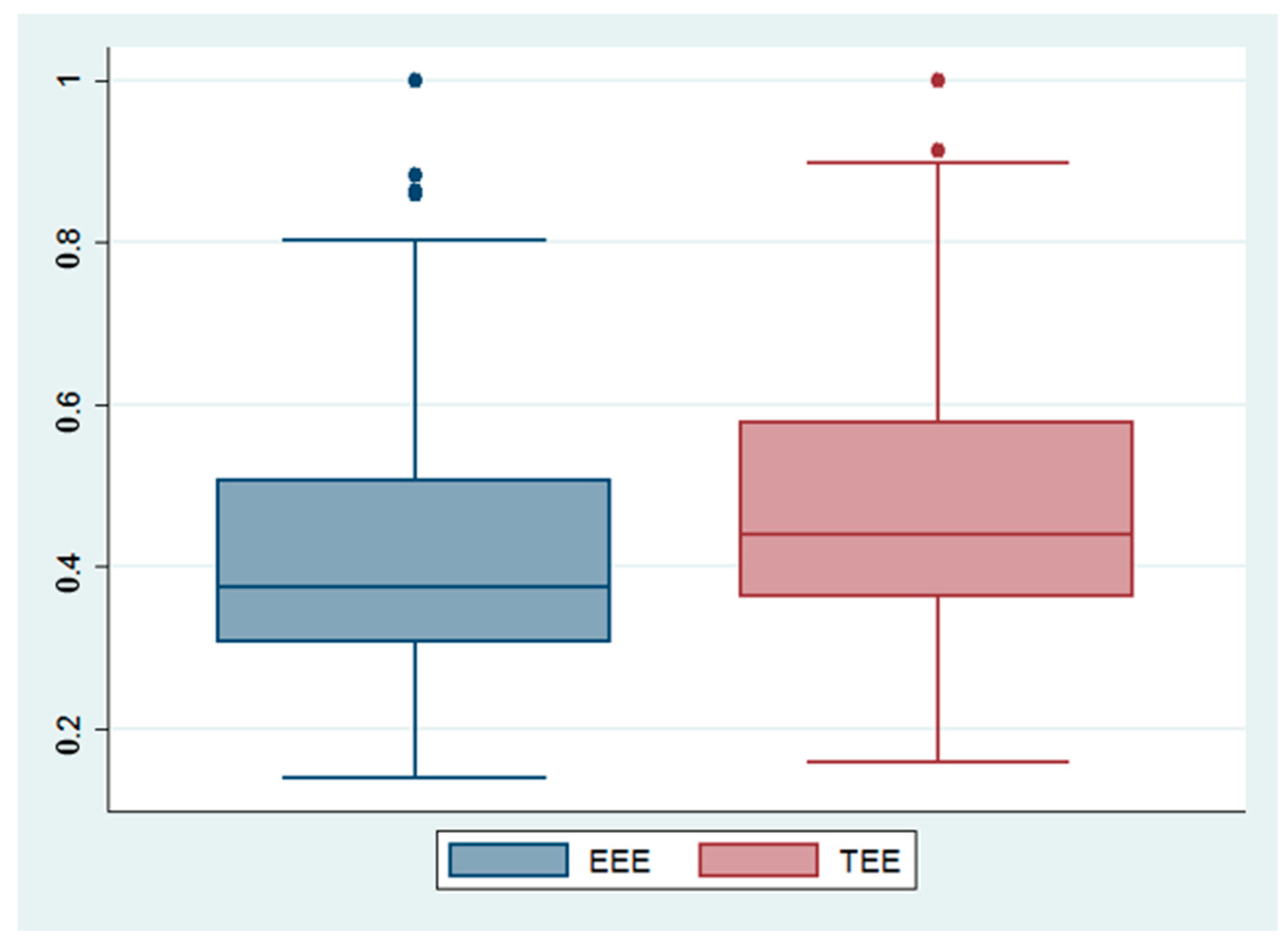
Meanwhile, since the EEE and TEE values did not show a large difference, we conducted a Mann-Whitney test to check the null hypothesis of no group difference. As shown in Table 5 and Figure 3, the M-W test statistic shows a p-value of 0.011, and we can reject the null hypothesis, concluding a significant group difference between TEE and EEE. This result means that TEE overestimates its real efficiency, including the environmental pollution effect, since emitting GHG is inevitable in production. Thus, in E and E studies, it is meaningful to consider undesirable output in order to obtain an unbiased sustainable efficiency value.
Meanwhile, this study also evaluates the difference in efficiency measurement between the radial DDF and non-radial approaches. With the same data, the results of radial DDF efficiency are shown in Table 6. Compared to non-radial SBM efficiency, we can see that the efficiency calculated by the radial DDF in Table 6 is much higher than the non-radial SBM efficiency in Table 4. Thus, we could deduce that the radial DDF result is surely an overestimation when compared to the result from SBM. The reason for this overestimation stems from the characteristics of the non-radial approach of SBM and, thus, it could be better to obtain the unbiased potentials from the non-radial SBM.
Figure 4 shows the graphs of the 3 efficiencies (EEE, TEE, and radial DDF efficiency). As mentioned, TEE, which does not consider undesirable output overestimates the efficiency value compared to EEE, which contains undesirable output. The radial DDF efficiency is higher than both TEE and EEE, implying an overly overestimated efficiency with much less potential.
3.3. Efficiency Decomposition
In this chapter, on the basis of Equation (6), we decompose EEE into PEE and SE. As explained above, PEE is the efficiency obtained from the VRS condition. SE (scale efficiency) is the ratio between energy efficiency under the CRS and VRS conditions. From this process, we could the classify DMUs’ returns to scale status. The result is shown in Table 7.
In the results, we can see that the average value of PEE, which is derived from VRS, is higher than that of EEE. This result stems from the fact that SE was excluded from EEE. When SE is close to 1, it means that the inefficiency caused by scale decreases, and if SE is close to 0, the inefficiency caused by scale is larger. Therefore, the value of SE is important for the firm when deciding green investment and considering its effectiveness. Although the Korean steel industry’s SE did not show a drastic fall, it still shows that 30–40% of the inefficiency can be improved through green investments. To improve each inefficient DMU’s efficiency value, it is through checking their RTS that it is possible to delineate a specific plan. RTS, which is classified as CRS, DRS, and IRS, is obtained from the following step.
All DMUs could be evaluated with their initial stage of CRS by linear programming. Assume that there are DMUs, and each DMU uses as its inputs to produce as its outputs. Then, the efficiency from the production scale could be defined in its linear form:
In this equation, each x and y is the vector of DMU’s inputs and outputs. λ is the weights vector. The function’s value of θ is the EEE. When θ = 1, this means the DMU is efficient; when θ < 1, this means an inefficient DMU that uses more input (1 − θ) compared to the other DMUs. In addition, it is possible to check RTS by using the sum of λ values calculated from the above equation. If = 1, DMU is on CRS (constant returns to scale), and this means both EEE and PEE are 1. Hence, firms showing CRS have an efficient input and output structure. On the other hand, if the firms’ scale efficiency is less than 1, this means that the firms’ input and output structure has not achieved full scale efficiency. In this case, when Σλ < 1, DMUs are on decreasing returns to scale (DRS), whereas when Σλ > 1, DMUs are on increasing returns to scale (IRS). Results of the RTS of the steel industry for five years are shown in Table 8.
In the Korean steel industry, the firms with IRS comprise a large majority. The number of firms with DRS is 3–5 in each year. IRS means that the rate of increased output is higher than that of input, implying that the increasing scale could enhance the DMU’s efficiency value. On the other hand, firms showing DRS can increase their efficiency by reducing their input structure or facilities. Since most Korean steel firms show IRS, the Korean government should promote green investments with incentives for the steel firms to increase their efficiency through expanding their scale.
3.4. Benchmark for Ineffective Firms
Since it is not easy for the steel industry to further reduce its GHG emissions, the Korean government should support the firms’ learning more from the industry’s benchmark cases among the firms on the production frontier to overcome the challenge of emissions reduction. Regarding the causes of inefficiency, since PEE and SE are evenly distributed, both the scale condition and intra-firm operation should be examined in more detail for the inefficient firms of the steel industry. To enhance individual firms’ performance, the result of benchmark cases could provide valuable information regarding each firm’s input target. As mentioned above, SBM-DEA provides the benchmark information for ineffective DMUs that do not show a “constant returns to scale” status. These firms can learn from the detailed information of efficient DMUs: each inefficient DMUs can take the learning effect from matching efficient DMU called the “reference set”. This reference set is allocated to inefficient DMUs when they have similar input and output structure. For an inefficient DMU to enhance its efficiency, its input target should achieve the value derived from Equation (7). The λ value could be defined as the level of influence of how much efficient DMUs give to each inefficient DMU. All the firms with EEE less than 1 can obtain benchmark information using Equation (7). Each projection target of an inefficient firm can be from the Equation (7). For example, SeAH Besteel’s target value the can come from the input value of SeAH Steel: 12 × 1.320007; by the same token, KOSTEEL’s target value can result from POSCO C and C: 11 × 0.065857 + SeAH Steel 12’s input value × 0.189196. The result of the benchmark information is derived in Table 9 under the CRS condition.
Reference set’s input × λ = inefficient DMU’s input target
Benchmark information is calculated based on 2011, because the efficient DMUs are very biased in 2011 and the average efficiency is also higher than that of the next four years. In the result, we can see that DONGKUK Steel, POSCO, POSCO C and C, YK steel, and SeAH Steel are the efficient DMUs among 20 firms, and SeAH Steel is the best DMU in that it appears 90 times as a reference set. This is because among the 20 firms in the sample of this study, SeAH Steel’s input and output structure would be similar to that of other inefficient DMUs. On the other hand, efficient DMUs that are not reported as a reference set as much as SeAH Steel means that their input and output structure is more different from that of other inefficient DMUs. Hence, from the benchmark information, inefficient DMUs should follow the structure of the reference set benchmark firm to enhance their efficiency, through the learning effect based on their allocated reference set.
Meanwhile, it could be speculated that the reason SeAH Steel is an exemplary DMU stems from the high demand for steel pipes. In 2011, in accordance with the expanding LNG market in the U.S, the demand for steel pipes had drastically increased and SeAH Steel, which has 12% of the domestic share of steel pipes, realized a large profit, and that may have affected its enhanced efficiency as a reference set.
4. Conclusions
In this study, we analyzed the efficiency of the Korean steel industry while considering undesirable output. We calculated diverse types of efficiencies and a series of empirical results for five years with 20 firms covered by Korea’s ETS. It is noteworthy that the enforcement of ETS policies is too loose to capture the regulation effects. Nonetheless, the paper sheds light on the appropriateness of the diverse approaches and the implications of these approaches. The SBM model with undesirable outputs is the core model for the comparison of the feasibility, and undesirable-DDF models were added for practical implications. We draw the results of diverse efficiencies, such as TEE, EEE, and EEE by radial DDF, with flexible mechanisms on returns to scale status and benchmark information for a catch-up effect. Major findings with practical implications from this study are summarized below.
First, we found that the EEE of 20 steel firms exhibits a decreasing trend across the span of five years. Even if there has been a short upturn in 2014 due to the exchange rate fluctuation coming from the global economic crisis, the trend, in general, clearly shows a downturn of the EEE. Since the Porter hypothesis strongly supports the regulation policies for enhancing efficiency, our results imply that government regulation is not enough for the firms to react in addition to the regulation. For example, Samsung Electronics Co., the most representative Korean company, paid millions of dollars in penalties for three years since the inauguration of the ETS in 2015. The relaxed target of 100% allowances for the participating companies in the first stage of the ETS could not encourage the covered companies to invest in green technology. Therefore, it seems that strong regulation is needed to enhance the sustainable performance of ETS, according to the Porter hypothesis. TEE always exhibits a higher value than EEE because TEE does not consider undesirable output of GHGs. Thus, it is reasonable to include undesirable output in a more systematic way to prevent this kind of overestimated bias. On the other hand, there is no systematic relationship between TEE and EEE, implying that GHGs are not the sole reason causing the firms’ higher inefficiency. Therefore, changes in intra-company governance, production structure, and technical innovation are required for firms to overcome the aggravating inefficiency in the steel industry over time.
Second, from the perspective of returns to scale, almost all firms show IRS, implying that the Korean steel industry has room to increase its overall industrial efficiency through an increase in scale. Therefore, it is certain that the potential efficiency shall increase if there is enough green investment. Meanwhile, as you can see in the SeAH Steel case, if a firm is competitive on its own, it may maintain a high efficiency regardless of regulation. Thus, each firm should make efforts to enhance their own competitiveness for their sustainable performance. Of course, this kind of scale upgrading may require higher emissions targets and, thus, the government should promote a balanced green investment of the covered companies between enhanced efficiency and newly-added responsibility [26]. It is noteworthy that upgrading the scale may not only arise from green investment, but also from organizational culture and/or behavioral changes in the private sectors. For this purpose, this paper showed the optimal leaning path of the inefficient firms toward their individual benchmark reference sets. Well-provided benchmark information can be helpful for guiding the efficiency enhancement of inefficient firms. Thus, each inefficient firm needs to refer to its unique benchmark reference set for its sustainable performance. Most of all, the covered companies should participate in the ETS not with a passive, critical, cost-saving attitude, but with a more proactive partnership, to lead the new international norms of sustainable development.
Acknowledgments
This paper is supported by the National Research Foundation of Korea Grant (NRF-2017K2A9A2A06013582) and by the National Natural Science Foundation of China (71603102, 71711540308).
Author Contributions
Yongrok Choi organized the models and finalized the paper, Yanni Yu helped the methodology, and Hyoung Seok Lee collected, analyzed the data, and prepared the first draft.
Conflicts of Interest
The authors declare no conflict of interest.
Appendix A

Table A1.
The industries and the number of covered companies in the Korean ETS.
| Industry | Number of Companies | Industry | Number of Companies |
|---|---|---|---|
| Construction | 40 | Textiles | 15 |
| Mining | 2 | Water | 3 |
| Machinery | 19 | Cement | 25 |
| Wood processing | 7 | Glass | 24 |
| Electronic, displays, and semiconductors | 45 | Food and drink | 23 |
| Power and energy | 38 | Car manufacturing | 24 |
| Nonmetallic | 24 | Oil refining | 4 |
| Petrochemical | 85 | Paper | 44 |
| Shipbuilding | 8 | Steel | 40 |
| Telecommunications | 6 | Waste | 44 |
| Aviation | 5 | Total | 525 |
Table A2.
Carbon allocation for each industry in the Korean ETS.
| Sector | Industry | Commitment Period | Three-Year Total | |||
|---|---|---|---|---|---|---|
| 2015 | 2016 | 2017 | ||||
| Total amount of emissions | 573,460,132 | 562,183,138 | 550,906,142 | 1,686,549,412 | ||
| Pre-allocated quota | 543,227,433 | 532,575,917 | 521,924,398 | 1,597,727,748 | ||
| Reserve | 88,821,664 | |||||
| Electricity | Power & Energy | 250,189,874 | 245,284,190 | 240,378,507 | 735,852,571 | |
| Industry | Mining | 245,386 | 240,575 | 235,763 | 721,724 | |
| Food and drink | 2,534,679 | 2,484,980 | 2,435,280 | 7,454,939 | ||
| Textile | 4,701,454 | 4,609,269 | 4,517,084 | 13,827,807 | ||
| Wood | 384,051 | 376,521 | 368,990 | 1,129,562 | ||
| Paper | 7,630,496 | 7,480,879 | 7,331,261 | 22,442,636 | ||
| Oil refining | 19,153,420 | 18,777,862 | 18,402,305 | 56,333,587 | ||
| Petro-chemical | 48,857,291 | 47,899,305 | 46,941,318 | 143,697,914 | ||
| Glass | 6,263,680 | 6,140,863 | 6,018,046 | 18,422,589 | ||
| Cement | 43,518,651 | 42,665,344 | 41,812,037 | 127,996,032 | ||
| Steel | General | 103,284,517 | 101,259,331 | 99,234,144 | 303,777,992 | |
| F-gas products | 675,361 | 662,119 | 648,877 | 1,986,357 | ||
| Non-ferrous | 6,888,332 | 6,753,266 | 6,618,201 | 20,259,799 | ||
| Machine | 1,416,225 | 1,388,456 | 1,360,687 | 4,165,368 | ||
| Semi Con. | General | 8,252,756 | 8,090,937 | 7,929,118 | 24,272,811 | |
| F-gas products | 2,202,049 | 2,158,871 | 2,115,694 | 6,476,614 | ||
| Display | General | 6,705,480 | 6,574,000 | 6,442,520 | 19,722,000 | |
| F-gas products | 2,438,238 | 2,390,430 | 2,342,621 | 7,171,289 | ||
| Electronics | 2,877,479 | 2,821,058 | 2,764,637 | 8,463,174 | ||
| Cars | 4,242,789 | 4,159,597 | 4,076,405 | 12,478,791 | ||
| Ship-building | 2,683,132 | 2,630,522 | 2,577,911 | 7,891,565 | ||
| Building | Building | 4,017,219 | 3,938,450 | 3,859,681 | 11,815,350 | |
| Telecommunication | 3,089,243 | 3,028,670 | 2,968,096 | 9,086,009 | ||
| Transportation | Air transportation | 1,289,780 | 1,264,490 | 1,239,201 | 3,793,471 | |
| Public & waste | Water | 766,351 | 751,324 | 736,298 | 2,253,973 | |
| Waste | 8,919,500 | 8,744,608 | 8,569,716 | 26,233,824 | ||
References
- Martin, R.; Muuls, M.; Wagner, U.J. The Impact of the European Union Emissions Trading Scheme on Regulated Firms: What Is the Evidence after Ten Years? Rev. Environ. Econ. Policy 2016, 10, 129–148. [Google Scholar] [CrossRef]
- Oestreich, A.M.; Tsiakas, I. Carbon Emissions and Stock Returns: Evidence from the EU Emissions Trading Scheme. J. Bank. Financ. 2015, 58, 294–308. [Google Scholar] [CrossRef]
- Choi, Y.; Liu, Y.; Lee, H. The economy impacts of Korean ETS with an emphasis on sectoral coverage based on a CGE approach. Energy Policy 2017, 109, 835–844. [Google Scholar] [CrossRef]
- Zhang, N.; Choi, Y. A note on the evolution of directional distance function and its development in energy and environmental studies 1997–2013. Renew. Sustain. Energy Rev. 2014, 33, 50–59. [Google Scholar] [CrossRef]
- Wang, K.; Che, L.; Ma, C.; Wei, Y.M. The shadow price of CO2 emissions in China’s iron and steel industry. Sci. Total Environ. 2017, 598, 272–281. [Google Scholar] [CrossRef] [PubMed]
- Che, L. Shadow Price Estimation of CO2 in China’s Regional Iron and Steel Industry. Energy Procedia 2017, 105, 3125–3131. [Google Scholar] [CrossRef]
- Kuosmanen, T.; Kortelainen, M. Stochastic non-smooth envelopment of data: Semi-parametric frontier estimation subject to shape constraints. J. Prod. Anal. 2012, 38, 11–28. [Google Scholar] [CrossRef] [Green Version]
- Charnes, A.; Cooper, W.W.; Rhodes, E. Measuring the efficiency of decision-making units. Eur. J. Oper. Res. 1978, 2, 429–444. [Google Scholar] [CrossRef]
- Zhang, N.; Kong, F.; Kung, C.-C. On Modeling Environmental Production Characteristics: A Slacks-Based Measure for China’s Poyang Lake Ecological Economics Zone. Comput. Econ. 2015, 46, 389–404. [Google Scholar] [CrossRef]
- Zhang, X.G.; Zhang, S. Technical Efficiency in China’s Iron and Steel Industry: Evidence from the new census data. Int. Rev. Appl. Econ. 2001, 15, 199–211. [Google Scholar] [CrossRef]
- Yang, W.; Shi, J.; Qiao, H.; Shao, Y.; Wang, S. Regional technical efficiency of Chinese Iron and steel industry based on bootstrap network data envelopment analysis. Soc.-Econ. Plann. Sci. 2017, 57, 14–24. [Google Scholar] [CrossRef]
- Wei, Y.-M.; Liao, H.; Fan, Y. An empirical analysis of energy efficiency in China’s iron and steel sector. Energy 2007, 32, 2262–2270. [Google Scholar] [CrossRef]
- Cho, B. Efficiency and Total Factor Productivity of North-East Asian Countries’ Steel Industries. Northeast Asia Econ. Stud. Korean 2008, 20, 1–24. [Google Scholar]
- Sheng, Y.; Song, L. Re-estimation of firms’ total factor productivity in China’s iron and steel industry. China Econ. Rev. 2013, 24, 177–188. [Google Scholar] [CrossRef]
- Lee, H.-S.; Kim, K.-S. Measuring Efficiency of Korean Steel Industry Employing DEA. J. Korea Contents Assoc. 2007, 7, 195–205. [Google Scholar] [CrossRef]
- Ha, C. A study on the efficiency of Korean steel industry using a DEA Model: Focused on technological innovation aspects. J. Inf. Technol. 2012, 11, 7–20. [Google Scholar]
- Zhou, P.; Ang, B.W.; Wang, H. Energy and CO2 emission performance in electricity generation: A non-radial directional distance function approach. Eur. J. Oper. Res. 2012, 221, 625–635. [Google Scholar] [CrossRef]
- Fukuyama, H.; Weber, W.L. A directional slacks-based measure of technical inefficiency. Soc.-Econ. Plan. Sci. 2009, 43, 274–287. [Google Scholar] [CrossRef]
- Choi, Y.; Zhang, N.; Zhou, P. Efficiency and abatement costs of energy-related CO2 emissions in China: A slacks-based efficiency measure. Appl. Energy 2012, 98, 198–208. [Google Scholar] [CrossRef]
- Tone, K. A slacks-based measure of efficiency in data envelopment analysis. Eur. J. Oper. Res. 2001, 130, 498–509. [Google Scholar] [CrossRef]
- Cooper, W.W.; Seiford, L.M.; Tone, K. Data Envelopment Analysis: A Comprehensive Text with Models, Applications, References and DEA-Solver Software; Springer: New York, NY, USA, 2007. [Google Scholar]
- Zhang, N.; Choi, Y. Environmental energy efficiency of China’s regional economies: A non-oriented slacks-based measure analysis. Soc. Sci. J. 2013, 50, 225–234. [Google Scholar] [CrossRef]
- Hu, J.L.; Wang, S.C. Total-factor energy efficiency of regions in China. Energy Policy 2006, 34, 3206–3217. [Google Scholar] [CrossRef]
- Banker, R.D.; Charnes, A.; Cooper, W.W. Some models for estimating technical and scale inefficiencies in data envelopment analysis. Manag. Sci. 1984, 30, 1078–1092. [Google Scholar] [CrossRef]
- Wei, C.; Ni, J.; Sheng, M. China’s energy inefficiency: A cross-country comparison. Soc. Sci. J. 2011, 48, 478–488. [Google Scholar] [CrossRef]
- Choi, Y.; Lee, H.S. Are Emissions Trading Policies Sustainable? A Study of the Petrochemical Industry in Korea. Sustainability 2016, 8, 1110. [Google Scholar] [CrossRef]
Figure 1.
Trend of the revenue and GHG emissions in the steel industry

Figure 2.
Graphical illustration of radial efficiency measure vs. SBM-efficiency measure.
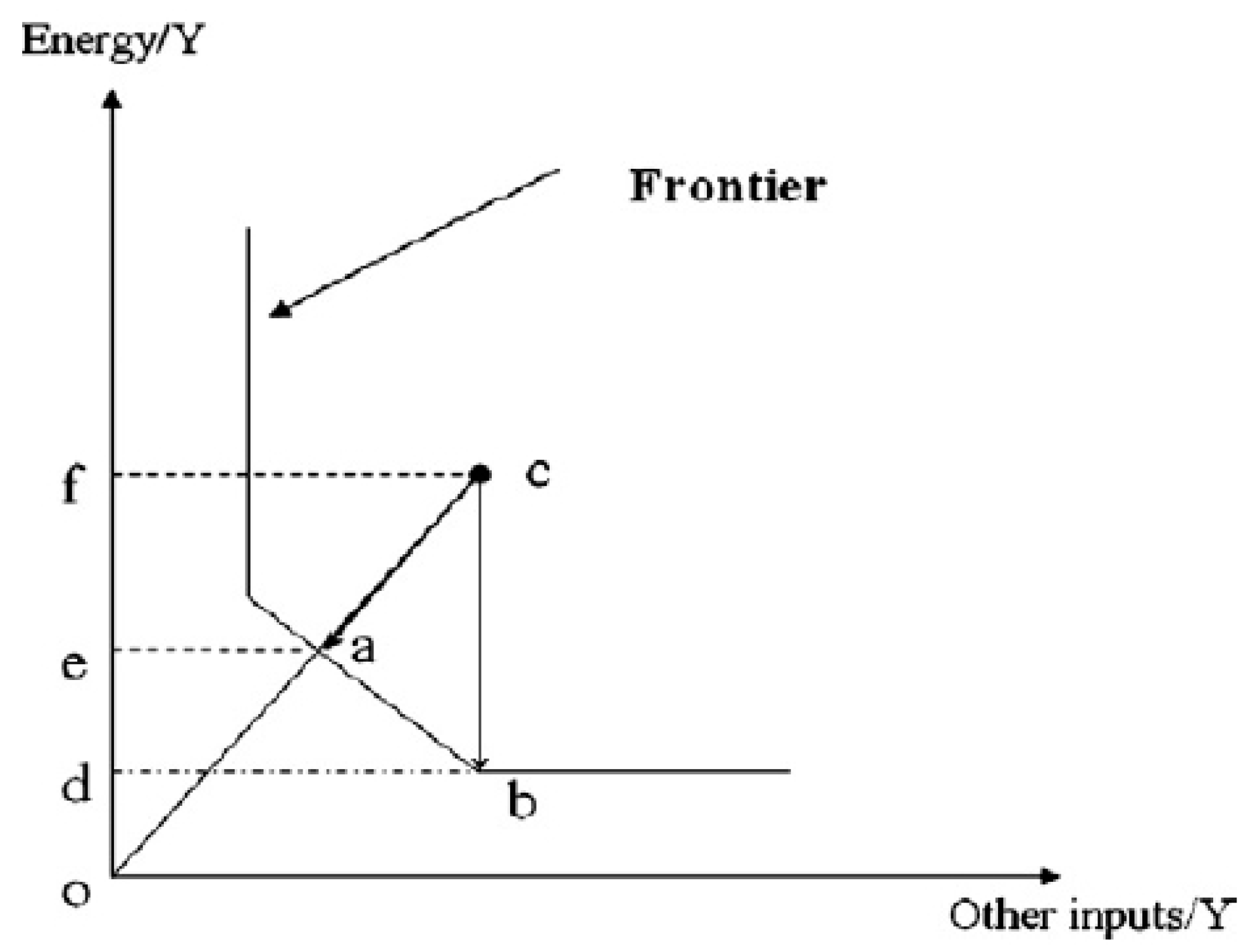
Figure 3.
Box plot of EEE vs. TEE.

Figure 4.
Trend of the three efficiencies.
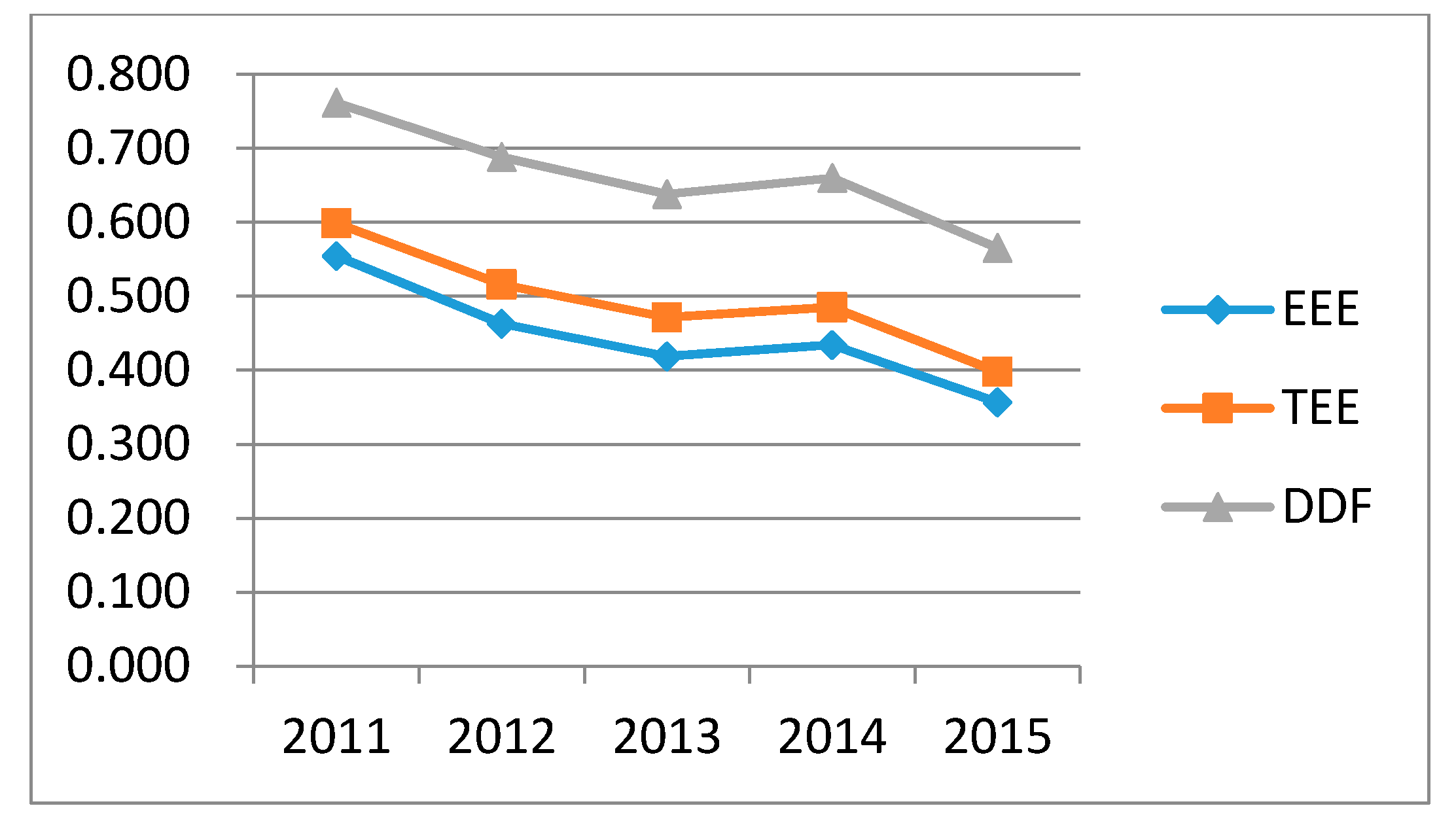
Table 1.
Revenue and GHG emissions data for firms in the steel industry (based on sample data of this study).
Table 1.
Revenue and GHG emissions data for firms in the steel industry (based on sample data of this study).
| 2011 | 2012 | 2013 | 2014 | 2015 | |
|---|---|---|---|---|---|
| Turnover (billion USD) | 662 | 597.8 | 540.7 | 567.7 | 470.6 |
| GHG (CO2 equivalent million tons) | 101.1 | 99.1 | 97.7 | 103.7 | 100.2 |
Table 2.
Descriptive statistics.
| Variable | Type | Unit | Mean | Max | Min. |
|---|---|---|---|---|---|
| Turnover | Desirable output | Million USD | 3281.5 | 39,171.7 | 91.3 |
| Carbon | Undesirable output | CO2 eq. tons | 501,786,317 | 77,124,639 | 32,533 |
| Capital | Input | Million USD | 105 | 577.2 | 4.1 |
| Labor | Input | Per person | 1968.75 | 17,877 | 152 |
| Energy | Input | Tera joules (TJ) | 53,519.7 | 863,564 | 630 |
Sources: Greenhouse Gas Inventory & Research Center of Korea (http://www.gir.go.kr/); DART: Data Analysis, Retrieval, and Transfer System (http://dart.fss.or.kr/).
Table 3.
Input and output correlation matrix.
| Variable | Energy | Capital | Labor | Turnover | GHG |
|---|---|---|---|---|---|
| Energy | 1 | ||||
| Capital | 0.647 * | 1 | |||
| Labor | 0.944 * | 0.752 * | 1 | ||
| Turnover | 0.970 * | 0.731 * | 0.981 * | 1 | |
| GHG | 0.940 * | 0.595 * | 0.951 * | 0.964 * | 1 |
* Statistically significant at the 95% confidence level.
Table 4.
Environment energy efficiency (with pollution) and traditional energy efficiency (without pollution) by SBM.
Table 4.
Environment energy efficiency (with pollution) and traditional energy efficiency (without pollution) by SBM.
| 2011 | 2012 | 2013 | 2014 | 2015 | ||||||
|---|---|---|---|---|---|---|---|---|---|---|
| EEE | TEE | EEE | TEE | EEE | TEE | EEE | TEE | EEE | TEE | |
| SIMPAC | 0.251 | 0.322 | 0.250 | 0.318 | 0.175 | 0.222 | 0.182 | 0.231 | 0.144 | 0.181 |
| SeAH Besteel | 0.314 | 0.377 | 0.269 | 0.320 | 0.269 | 0.321 | 0.279 | 0.336 | 0.222 | 0.265 |
| SeAH Steel | 1.000 | 1.000 | 1.000 | 1.000 | 0.859 | 0.869 | 1.000 | 1.000 | 0.796 | 0.733 |
| KISWIRE | 0.375 | 0.404 | 0.342 | 0.365 | 0.334 | 0.359 | 0.359 | 0.386 | 0.294 | 0.308 |
| DAEHAN Steel | 0.411 | 0.503 | 0.430 | 0.528 | 0.432 | 0.528 | 0.463 | 0.567 | 0.363 | 0.442 |
| DONGKUK Steel | 1.000 | 1.000 | 0.566 | 0.623 | 0.373 | 0.473 | 0.357 | 0.435 | 0.309 | 0.391 |
| DONGBU Steel | 0.436 | 0.503 | 0.396 | 0.456 | 0.374 | 0.436 | 0.526 | 0.573 | 0.502 | 0.529 |
| DONGIL | 0.459 | 0.579 | 0.396 | 0.502 | 0.354 | 0.447 | 0.346 | 0.438 | 0.287 | 0.360 |
| YEONGHWA Metal | 0.146 | 0.169 | 0.138 | 0.159 | 0.140 | 0.161 | 0.176 | 0.195 | 0.164 | 0.182 |
| DONGBU Metal | 0.375 | 0.487 | 0.335 | 0.435 | 0.319 | 0.414 | 0.307 | 0.399 | 0.241 | 0.313 |
| POSCO | 1.000 | 1.000 | 0.594 | 0.735 | 0.473 | 0.620 | 0.484 | 0.637 | 0.444 | 0.584 |
| POSCO C&C | 1.000 | 1.000 | 0.785 | 0.804 | 0.787 | 0.808 | 0.803 | 0.818 | 0.592 | 0.625 |
| KISCO | 0.311 | 0.378 | 0.309 | 0.375 | 0.305 | 0.373 | 0.288 | 0.351 | 0.243 | 0.296 |
| HYUNDAI BNG Steel | 0.563 | 0.552 | 0.495 | 0.480 | 0.495 | 0.480 | 0.515 | 0.497 | 0.486 | 0.457 |
| HYUNDAI Steel | 0.488 | 0.618 | 0.455 | 0.575 | 0.341 | 0.427 | 0.433 | 0.546 | 0.332 | 0.417 |
| HWANYOUNG Steel | 0.359 | 0.442 | 0.322 | 0.396 | 0.295 | 0.362 | 0.253 | 0.308 | 0.230 | 0.281 |
| YK Steel | 1.000 | 1.000 | 0.883 | 0.912 | 0.862 | 0.898 | 0.765 | 0.824 | 0.494 | 0.607 |
| KOSTEEL | 0.534 | 0.578 | 0.436 | 0.470 | 0.404 | 0.430 | 0.375 | 0.390 | 0.297 | 0.292 |
| DONGKUK Industry | 0.558 | 0.507 | 0.515 | 0.463 | 0.441 | 0.399 | 0.445 | 0.389 | 0.413 | 0.360 |
| Kiswire | 0.510 | 0.554 | 0.342 | 0.407 | 0.340 | 0.404 | 0.332 | 0.389 | 0.289 | 0.335 |
| Average | 0.554 | 0.599 | 0.463 | 0.516 | 0.419 | 0.471 | 0.434 | 0.485 | 0.357 | 0.398 |
Table 5.
Result of the Mann-Whitney test.
| Test | Null Hypothesis | Test Statistic | p-Value |
|---|---|---|---|
| Wilcoxon-Mann-Whitney | Mean (EEE) = Mean (TEE) | 4731 | 0.011 |
Table 6.
Environment energy efficiency (with pollution) using a radial DDF.
| 2011 | 2012 | 2013 | 2014 | 2015 | |
|---|---|---|---|---|---|
| SIMPAC | 0.470 | 0.458 | 0.316 | 0.337 | 0.258 |
| SeAH Besteel | 0.597 | 0.504 | 0.508 | 0.538 | 0.419 |
| SeAH Steel | 1.000 | 1.000 | 0.899 | 1.000 | 0.955 |
| KISWIRE | 0.584 | 0.517 | 0.524 | 0.558 | 0.408 |
| DAEHAN Steel | 0.725 | 0.755 | 0.742 | 0.820 | 0.635 |
| DONGKUK Steel | 1.000 | 0.853 | 0.704 | 0.706 | 0.584 |
| DONGBU Steel | 0.781 | 0.716 | 0.686 | 0.852 | 0.837 |
| DONGIL | 0.858 | 0.760 | 0.671 | 0.657 | 0.543 |
| YEONGHWA Metal | 0.236 | 0.231 | 0.235 | 0.256 | 0.237 |
| DONGBU Metal | 0.676 | 0.607 | 0.584 | 0.573 | 0.497 |
| POSCO | 1.000 | 0.897 | 0.792 | 0.840 | 0.696 |
| POSCO C&C | 1.000 | 0.919 | 0.925 | 0.929 | 0.819 |
| KISCO | 0.570 | 0.574 | 0.591 | 0.558 | 0.471 |
| HYUNDAI BNG Steel | 0.792 | 0.692 | 0.697 | 0.714 | 0.675 |
| HYUNDAI Steel | 0.768 | 0.669 | 0.512 | 0.660 | 0.520 |
| HWANYOUNG Steel | 0.735 | 0.660 | 0.605 | 0.508 | 0.468 |
| YK Steel | 1.000 | 0.970 | 0.978 | 0.920 | 0.777 |
| KOSTEEL | 0.836 | 0.671 | 0.585 | 0.533 | 0.401 |
| DONGKUK Industry | 0.718 | 0.673 | 0.570 | 0.613 | 0.570 |
| Kiswire | 0.888 | 0.638 | 0.638 | 0.552 | 0.537 |
| Average | 0.762 | 0.688 | 0.638 | 0.660 | 0.565 |
Table 7.
Pure technical efficiency score (VRS) and scale efficiency using SBM.
| 2011 | 2012 | 2013 | 2014 | 2015 | ||||||
|---|---|---|---|---|---|---|---|---|---|---|
| PEE | SE | PEE | SE | PEE | SE | PEE | SE | PEE | SE | |
| SIMPAC | 1.000 | 0.251 | 1.000 | 0.250 | 0.748 | 0.234 | 1.000 | 0.182 | 1.000 | 0.144 |
| SeAH Besteel | 0.426 | 0.739 | 0.314 | 0.856 | 0.309 | 0.869 | 0.351 | 0.796 | 0.225 | 0.990 |
| SeAH Steel | 1.000 | 1.000 | 1.000 | 1.000 | 0.872 | 0.985 | 1.000 | 1.000 | 1.000 | 0.796 |
| KISWIRE | 0.485 | 0.773 | 0.421 | 0.812 | 0.409 | 0.817 | 0.440 | 0.816 | 0.343 | 0.857 |
| DAEHAN Steel | 0.504 | 0.816 | 0.543 | 0.793 | 0.539 | 0.801 | 0.575 | 0.804 | 0.432 | 0.840 |
| DONGKUK Steel | 1.000 | 1.000 | 0.797 | 0.710 | 0.631 | 0.590 | 0.541 | 0.659 | 0.577 | 0.536 |
| DONGBU Steel | 0.837 | 0.520 | 0.720 | 0.550 | 0.647 | 0.578 | 0.630 | 0.835 | 0.505 | 0.995 |
| DONGIL | 1.000 | 0.459 | 0.839 | 0.473 | 0.742 | 0.477 | 0.709 | 0.488 | 0.627 | 0.457 |
| YEONGHWA Metal | 1.000 | 0.146 | 0.384 | 0.359 | 1.000 | 0.140 | 0.385 | 0.456 | 0.343 | 0.478 |
| DONGBU Metal | 0.480 | 0.780 | 0.431 | 0.778 | 0.418 | 0.764 | 0.412 | 0.746 | 0.330 | 0.729 |
| POSCO | 1.000 | 1.000 | 0.916 | 0.648 | 0.837 | 0.565 | 1.000 | 0.484 | 0.838 | 0.530 |
| POSCO C&C | 1.000 | 1.000 | 0.909 | 0.864 | 0.905 | 0.870 | 0.917 | 0.876 | 0.803 | 0.738 |
| KISCO | 0.395 | 0.789 | 0.330 | 0.936 | 0.342 | 0.893 | 0.322 | 0.894 | 0.271 | 0.896 |
| HYUNDAI BNG Steel | 0.712 | 0.791 | 0.623 | 0.794 | 0.636 | 0.778 | 0.653 | 0.789 | 0.628 | 0.774 |
| HYUNDAI Steel | 1.000 | 0.488 | 0.896 | 0.508 | 0.721 | 0.474 | 1.000 | 0.433 | 0.681 | 0.488 |
| HWANYOUNG Steel | 0.479 | 0.748 | 0.423 | 0.762 | 0.394 | 0.749 | 0.341 | 0.744 | 0.307 | 0.747 |
| YK Steel | 1.000 | 1.000 | 0.941 | 0.939 | 1.000 | 0.862 | 0.982 | 0.779 | 1.000 | 0.494 |
| KOSTEEL | 1.000 | 0.534 | 0.805 | 0.542 | 0.694 | 0.582 | 0.842 | 0.445 | 1.000 | 0.297 |
| DONGKUK Industry | 1.000 | 0.558 | 1.000 | 0.515 | 0.739 | 0.597 | 0.749 | 0.594 | 0.693 | 0.596 |
| Kiswire | 1.000 | 0.510 | 0.597 | 0.573 | 0.593 | 0.573 | 0.595 | 0.557 | 1.000 | 0.289 |
| Average | 0.816 | 0.695 | 0.694 | 0.683 | 0.659 | 0.660 | 0.672 | 0.669 | 0.630 | 0.652 |
Table 8.
RTS for DMU.
| 2011 | 2012 | 2013 | 2014 | 2015 | |
|---|---|---|---|---|---|
| RTS status | Constant = 5 | Constant = 1 | Constant = 0 | Constant = 1 | Constant = 0 |
| Decreasing = 3 | Decreasing = 5 | Decreasing = 5 | Decreasing = 5 | Decreasing = 3 | |
| Increasing = 12 | Increasing = 14 | Increasing = 15 | Increasing = 14 | Increasing = 17 | |
| Cause of inefficiency | PEE:7 | PEE:8 | PEE:9 | PEE:10 | PEE:11 |
| SE:8 | SE:11 | SE:11 | SE:9 | SE:9 |
Table 9.
Firms for benchmark (2011 case).
| Efficient DMU (Number of Reference Sets) | DMU | Efficiency | Benchmark (Lambda Value) |
|---|---|---|---|
| DONGKUK Steel 11 (2) POSCO 11 (1) POSCO C&C 11 (17) YK Steel 11 (5) SeAH Steel 11 (5) SeAH Steel 12 (56) SeAH Steel 14 (29) | SIMPAC | 0.251 | SeAH Steel 14 (0.168860) |
| SeAH Besteel | 0.314 | SeAH Steel 12 (1.320007) | |
| SeAH Steel | 1.000 | SeAH Steel 11(1.000000) | |
| KISWIRE | 0.375 | SeAH Steel 12 (0.433333) | |
| DAEHAN Steel | 0.411 | SeAH Steel 12 (0.624573) | |
| DONGKUK Steel | 1.000 | DONGKUK Steel 11 (1.000000) | |
| DONGBU Steel | 0.436 | POSCO C&C 11 (0.168500) | |
| SeAH Steel 12 (1.986135) | |||
| DONGIL | 0.459 | SeAH Steel 14 (0.282895) | |
| YEONGHWA Metal | 0.146 | SeAH Steel 12 (0.230944) | |
| DONGBU Metal | 0.375 | SeAH Steel 14 (0.491228) | |
| POSCO | 1.000 | POSCO 11 (1.000000) | |
| POSCO C&C | 1.000 | POSCO C&C 11 (1.000000) | |
| KISCO | 0.311 | SeAH Steel 12 (0.542191) | |
| HYUNDAI BNG Steel | 0.563 | SeAH Steel 12 (0.513083) | |
| HYUNDAI Steel | 0.488 | POSCO C&C 11 (12.422546) | |
| SeAH Steel 12 (1.796534) | |||
| HWANYOUNG Steel | 0.359 | SeAH Steel 12 (0.321957) | |
| YK Steel | 1.000 | YK Steel 11 (1.000000) | |
| KOSTEEL | 0.534 | POSCO C&C 11 (0.065857); | |
| SeAH Steel 12 (0.189196) | |||
| DONGKUK Industry | 0.558 | SeAH Steel 11 (0.308831) | |
| Kiswire | 0.510 | SeAH Steel 12 (0.034409) |
© 2018 by the authors. Licensee MDPI, Basel, Switzerland. This article is an open access article distributed under the terms and conditions of the Creative Commons Attribution (CC BY) license (http://creativecommons.org/licenses/by/4.0/).
Share and Cite
MDPI and ACS Style
Choi, Y.; Yu, Y.; Lee, H.S. A Study on the Sustainable Performance of the Steel Industry in Korea Based on SBM-DEA. Sustainability 2018, 10, 173. https://doi.org/10.3390/su10010173
AMA Style
Choi Y, Yu Y, Lee HS. A Study on the Sustainable Performance of the Steel Industry in Korea Based on SBM-DEA. Sustainability. 2018; 10(1):173. https://doi.org/10.3390/su10010173
Chicago/Turabian StyleChoi, Yongrok, Yanni Yu, and Hyoung Seok Lee. 2018. "A Study on the Sustainable Performance of the Steel Industry in Korea Based on SBM-DEA" Sustainability 10, no. 1: 173. https://doi.org/10.3390/su10010173
Note that from the first issue of 2016, this journal uses article numbers instead of page numbers. See further details here.