Solving a More Flexible Home Health Care Scheduling and Routing Problem with Joint Patient and Nursing Staff Selection

Abstract

Development of an efficient and effective home health care (HHC) service system is a quite recent and challenging task for the HHC firms. This paper aims to develop an HHC service system in the perspective of long-term economic sustainability as well as operational efficiency. A more flexible mixed-integer linear programming (MILP) model is formulated by incorporating the dynamic arrival and departure of patients along with the selection of new patients and nursing staff. An integrated model is proposed that jointly addresses: (i) patient selection; (ii) nurse hiring; (iii) nurse to patient assignment; and (iv) scheduling and routing decisions in a daily HHC planning problem. The proposed model extends the HHC problem from conventional scheduling and routing issues to demand and capacity management aspects. It enables an HHC firm to solve the daily scheduling and routing problem considering existing patients and nursing staff in combination with the simultaneous selection of new patients and nurses, and optimizing the existing routes by including new patients and nurses. The model considers planning issues related to compatibility, time restrictions, contract durations, idle time and workload balance. Two heuristic methods are proposed to solve the model by exploiting the variable neighborhood search (VNS) approach. Results obtained from the heuristic methods are compared with a CPLEX based solution. Numerical experiments performed on different data sets, show the efficiency and effectiveness of the solution methods to handle the considered problem.

1. Introduction

1.1. Background

In general, growth in the HHC service industry is influenced by the increasing aging population, number of people with disabilities, rising health care costs and capacity issues at hospitals. Patients have different personal assistance requirements such as dressing, monitoring medicine dosage, daily physiotherapy, speech therapy, hospital or laboratory check-ups, etc. HHC services are quite simple and friendly for the patients as care is provided in their own home in a relaxed environment. The provision of health care services at home has been a rapidly developing area of the global economy in the last two decades, with more than 10,000 firms now providing therapeutic, rehabilitative and palliative services in the United States alone [1]. This is evident from the fact that many new organizations have been registered in this area of HHC in every developed country. In response to the increasing competitive pressures in all businesses, service providers must discover new ways to decrease their cost, improve quality and enhance productivity [2]. To achieve these objectives, service oriented businesses have to make rational decisions for obtaining new resources and increasing the utilization of existing resources. Hence, every HHC service system should be efficient, sustainable and flexible to incorporate the demand and supply patterns.

Scheduling and route planning is an important aspect of an HHC service system for managing daily operations, where caregivers (nurses) are assigned to patients under the restrictions related to the availability and compatibility. Generally, the HHC service problem is considered similar to the vehicle routing problem with time windows (VRPTW). Although it is similar, it contains many different constraints, which make it more complex and diverse from VRPTW. A large amount of work in the existing HHC service literature is about the assignment of patients to nurses, scheduling and route planning of nursing staff to minimize the total distance covered. Some authors have also discussed the districting based care strategy and continuity of care aspects [3,4,5], whereas other researchers focused on the quality of care and satisfaction level of patients and nurses. Much of the research is still limited to the development of scheduling and routing plans, where it is mandatory to assign all the available nurses to all the patients considered in the problem. Hence, the flexibility related to the recruitment of nursing staff, patient selection and integration of new patients and nursing staff in the existing HHC planning system is not jointly considered in the previous literature. Private HHC firms are similar to other types of commercial business entities, thus financial viability is necessary for their sustainability and growth. This situation demands the consideration of human resource recruitment following the total patient demand, where a firm only recruits the most necessary health care staff to meet the demand to avoid excess capacity and operational losses. Similarly, some new incoming patients may be referred to other home health care facilities in the case of capacity shortage or unavailability of required skills. Moreover, it is also economical for an HHC organization to refer new patients to other HHC firms, if they belong to a distant area that is not fully covered by the concerned HHC organization. Hence, it is very important to consider nurse hiring and patient selection decisions simultaneously along with scheduling and routing decisions to optimize the overall problem.

1.2. A Flexible HHC Planning Problem

The potential patients located at different geographical places can be seen similar to the candidate sites considered to open the facilities at different locations in the location routing problem (LRP). The selection of patients while making a routing decision is like the case of LRP, where facility location and vehicle routing decisions are considered in the same model to avoid suboptimal results. The interdependence between location and routing was first covered by Perl and Daskin [6]. They defined a warehouse location routing model that has the capability of simultaneously solving location and routing problems. Nagy and Salhi [7] also demonstrated that considering location and routing simultaneously can lead to better location solutions, which could result in substantial reduction in total travel costs. Facility location, allocation and routing decisions are simultaneously considered in the perspective of a multi-level supply chain network design by Lee et al. [8], whereas possible referral of a new patient to some other HHC firm and mandatory assignment of existing nurses and patients in the daily planning model over the period of their contract durations is similar to the dynamic facility location models proposed by Erlenkotter [9] and Shulman [10]. In these models, the option to open and close a facility is available for each facility in every time period over the planning horizon; however, a fixed cost is associated with such decisions. These models show flexibility to incorporate the changing demand and cost trends in the future and provide us motivation to develop HHC planning models considering similar features.

In real-life home health care problems, new patients and health care staff join the existing HHC service system on a daily basis. Therefore, home health care firms need to jointly consider the new patients and nursing staff along with existing individuals in the planning problem. This paper addresses a daily HHC planning problem, which considers the assignment, scheduling and routing decisions along with staff hiring and patient selection decisions. Moreover, the model formulation is flexible enough to handle the existing and new patients simultaneously along with previously hired and new nurses while maintaining their separate identity, so that the existing routes are optimized again on the inclusion of new patients in the daily planning system. In addition, when the routes of existing nurses and patients are again optimized along with new routes in the daily planning model, it gives effective and efficient routes in fluctuating health care demands. The HHC problem considered here has a home health care office as the origin and destination depot, where each route must start and end. The service required by each patient may be different, hence each nurse must possess a set of different skills. Every new nurse and patient indicate time windows when they are available for service appointments, along with available and required qualification, respectively. Nurse schedules should respect the maximum nurse working hours per day along with nurse and patient time windows, as well as qualification compatibility constraints. Each new nurse is either hired or reconsidered as a new nurse on the next planning days, but once hired, it is compulsory to assign a route to a nurse every day until her contract is over. Similarly, each new patient is either admitted, referred or sent to a waiting list for a certain number of weeks, but, once admitted, it is compulsory to assign a nurse to the existing patient every day until his/her contract duration comes to an end. However, the patients sent to a waiting list are reconsidered on the next planning day with the hope of an earlier admission. These decisions depend on the relevant costs associated with them. The expectation of a new patient arrival and departure of an existing patient against a particular service is the key factor for sending a patient to the waiting list. We developed an objective function that minimizes the cost associated with three sub objectives: (a) route cost (cost of nurse hiring and distance travelled), (b) nurse dissatisfaction cost (cost associated with idle time and work load difference), and (c) patient dissatisfaction cost (cost associated with patient referral and sending to waiting list).

1.3. Contributions

The main contribution of this paper is the development of a mathematical model that extends the previously studied HHC problems from joint assignment, scheduling and routing decisions to patient selection and staff hiring decisions. To the best of our knowledge, the integration issues of existing patients and healthcare staff with the new applicants are not tackled in the existing HHC scheduling and routing models. Our modelling approach is flexible enough to integrate the existing patients, waiting list patients and existing nursing staff with the new entrants in the daily planning model. Moreover, the proposed heuristic algorithms provide promising results by using the novel initial heuristic solution approach with the VNS based solution methods. Finally, the proposed mathematical model and solution approaches are useful for the sustainability of HHC operations. The integration of existing patients and nursing staff with the new entrants in the daily planning model in the perspective of capacity and demand requirements will enable the achievement of sustainable operational efficiency and long-term competitive advantage.

The rest of the paper is organized as follows: Section 2 describes the related work, Section 3 presents the problem description and mathematical model, Section 4 contains the solution approach and Section 5 details the computational experiments and results. The conclusions and future research options are discussed in Section 6.

2. Literature Review

Begur et al. [2] and Cheng and Rich [11] were among the first authors to study the HHC problem and begin using operation research for HHC planning problems. Begur et al. [2] developed a spatial decision support system for the scheduling and routing decisions in the United States to balance the workloads and minimize travel times. They integrated the PC-based GIS software with a scheduling heuristic to develop routes. The visual and interactive capability of the system allows users to see the nurse and patient locations, routes and generate what-if scenarios. The system is helpful for reducing the cost significantly in terms of manual paper work and travel costs. Cheng and Rich [11] extended the problem to include full time and part time nurses, introducing time windows for nurses and patients along with breaks for the nurses. The objective function was to minimize the cost associated with the work performed in overtime and part time. Two different MILP formulations were given based on double indexed variables and triple indexed variables, with the problem solved using a two-phase heuristic algorithm. Phase one builds parallel tours by generating several routes simultaneously and phase two improves the routes identified in phase one. Bertels and Fahle [12] studied a daily assignment and routing problem, developing a software package to solve the problem. In the package, a combination of linear programming, constraint programming, and meta heuristics were used to find solutions. The solution approach of the package interlinks two parts: determining an assignment of suitable patients to nurses and finding an optimal sequencing for each partition found in the first part. Daily scheduling and routing HHC problem with shared visits of more than one care taker was introduced by Thomsen [13]. He found the insertion heuristic based initial solution and then further improved the solution by using tabu search. Eveborn et al. [14] developed a decision support system called Laps Care, involving a health care organization in the development process. They presented a set partitioning formulation and a heuristic solution method was proposed using repeated matching approach. The solution method was used to solve the data instances with a maximum of 20 caretakers and 123 patients. Hertz and Lahrichi [15] developed an HHC model with a workload measure for nurses, taking into account the number of visits, patient level of need, travelling distances and a number of patients assigned in each category. A simplification of the proposed model by ignoring the case load makes it a mixed integer linear model, therefore solved using CPLEX. However, when the case load is also considered in the objective function, this nonlinear model is solved using a tabu search algorithm. Bredstrom and Ronnqvist [16] developed a mathematical model similar to VRPTW but with the capability of addressing the synchronization and precedence constraints between pairs of visits. These additional constraints tie the routes together and this model is solved using a heuristic solution method.

Medium-term HHC planning problems have been also addressed in the literature. A HHC problem based on patient care intervals over a planning horizon was proposed by An et al. [17]. The objective function minimizes the total travel time of nurses over the planning period. They introduced two phase heuristic algorithms and tested them using real data sets and randomly generated data instances of the problem. A medium-term home health care problem along with a metaheuristic solution method was devised by Trautsamwieser and Hirsch [18]. The authors proposed a branch-price and cut approach, which uses a VNS solution as the upper bounds. Shao et al. [19] studied the therapist routing and scheduling problem, proposing a MILP model which considers different patient categories, optional weekly treatment arrangements and a complex payment structure. The heuristic method developed by the authors, greedy randomized adaptive search procedure (GRASP), adopts a two-phase solution strategy. The first phase makes schedules by constructing the daily routes for therapists in parallel, then integrates these daily routes to form weekly schedules. A sophisticated neighborhood search method is performed to meet the local optimum in the second phase. A two-stage solution approach is proposed by Nickel et al. [20] for weekly optimal plans associated with mid-term and short-term HHC planning problems, namely master schedule problem and operational planning problem. The authors combined constraint programming with different metaheuristics to treat realistic constraints with flexibility. Rodriguez-Verjan et al. [21] proposed two MILP models considering strategic and tactical decisions for an HHC network design problem. The first model determines a strategic location plan for HHC centers while the second model covers a tactical management plan for each HHC center.

Despite a large amount of research related to HHC problems, most work focuses on scheduling and routing issues. Some authors also studied the HHC problem considering new patient assignment and the dynamic nature of patient arrival; however, they also missed the issues associated with patient selection, nurse recruitment and integration of new staff. Bennett and Erera [22] investigated the home health nurse routing and scheduling (HHNRS) problem, where new patients arrive dynamically and they must be visited following a given weekly frequency and fixed time windows. The objective function of the proposed model aims to maximize the number of patients attended per nurse per unit time while a rolling horizon myopic planning approach combined with new capacity based insertion heuristic is used to solve this problem. HHC staff dimensioning problem with uncertain demands was addressed by Rodriguez et al. [23]. An integer linear stochastic programming based two-stage approach is used to solve the problem by exploiting historical medical data. The home health care system was also explored in the context of a districting problem. Blais et al. [4] investigated a districting based HHC problem considering multiple criteria in modelling the problem and used a tabu search based approach to solve the problem. Starting from an initial solution, the algorithm moves a basic unit to an adjacent district or performs a full swap of two basic units. Benzarti et al. [3] developed two models for the districting problem that can be applied to the HHC problems. Mixed integer programming models contain the constraints related to indivisibility of basic units, compactness, work load balance and compatibility. The objective function of the models balances the work load and minimizes the total travel distance.

In addition, some scholars have also treated the HHC assignment and scheduling problems under the constraints of continuity of care. Continuity of care is one of the most important quality indicators related to the services provided by any health care facility [24]. Under the continuity of care, an HHC firm assigns only one nurse to a patient over a longer period of time. However, HHC firms need to maintain a balance between the continuity of care and service flexibility to achieve better operational efficiency. Lanzarone and Matta [25] proposed a patient assignment problem, which deals with the assignment of a newly admitted patient to the reference operator under the restrictions of continuity of care and uncertain workload. The policy suggested by the authors permits planners to allocate each new patient with a minimum increment of the expected cost sustained by the health care provider. Nurse-to-patient assignment with respect to continuity of care was studied by Carello and Lanzarone [5]. The authors developed a cardinality-constrained robust approach to modify the deterministic assignment model with the capability to consider uncertainty in patient demands without the need of generating scenarios. The results were promising, but the approach did not obtain optimal results for all the instances in a reasonable computational time. An integrated approach for the weekly planning of HHC services that jointly tackles the assignment, scheduling and routing decisions was proposed by Cappanera et al. [26]. The pattern based approach developed by the authors coordinates the diverse decision levels and under a hierarchical skill management policy, an operator with a particular skill is allowed to serve patients demanding lower level skills. The mathematical model formulations contain the continuity of care constraints and the model aims at balancing the workload among operators.

More recently, the HHC scheduling and routing problems have been studied by several authors considering different criteria. Trautsamwieser et al. [27] developed a home health care model in the context of natural disasters. The model minimizes total driving times, waiting times and the dissatisfaction level of both clients and nurses. Small problems are solved using the solver Xpress 7.0, while a VNS based heuristic method is used to solve real-life data instances. Rasmussen et al. [28] studied HHC problem from the perspective of preference constraints and temporal dependencies. They modelled the problem as a set partitioning problem. Considering different preferences, they introduced visit clustering schemes and developed a branch and price solution algorithm. An HHC problem with interdependent services was studied by Mankowska et al. [29]. They developed neighborhood search based efficient heuristic methods, capable of handling the synchronization requirements as well as large sized problems. Redjem and Marcon [30] proposed a heuristic method named as caregivers routing heuristic (CRH) to address the problem of caregivers routing. In first step, the heuristic method develops caregivers’ routes based on the shortest travel time, while the second step integrates the sequencing and coordination constraints to satisfy all the problem assumptions. The CRH performance shows its computational efficiency for real-life situations and unlike MILP approaches, it proved to be less sensitive to the temporal dependencies. Yalçındağ et al. [31] suggested a data driven approach to estimate the travel times for caregivers considering patient attributes. The proposed Kernel regression method estimates travel times using previous travel time information. The main advantage of their method is a two-stage approach. It assigns caregivers using travel time estimates in the first step and then successfully defines routes in the second stage. The authors also compared the performance of this two-stage approach using the Kernel regression method with joint assignment and routing solution methods. Du et al. [32] studied an HHC scheduling problem considering patients’ priorities and time windows constraints. The authors proposed a solution algorithm which combines genetic algorithm (GA) with local search to solve large-scale problems. Allaoua et al. [33] studied an HHC problem which aims to plan optimal schedules and routes for the health care staff. The authors developed an integer linear programming formulation to solve small instances while a matheuristic was proposed to solve the large instances. The proposed mathheuristic decomposes the earlier formulation into two problems and solves rostering and routing parts separately through an exact method.

Although a lot of research has been done considering HHC issues, the integration of existing HHC patients and care givers with newly arrived entrants (patients, nursing staff) did not get the attention of the researchers. This study aims to develop a flexible MILP model for the HHC scheduling and routing problem, incorporating three types of patients: (1) new patients, (2) existing patients, and (3) waiting list patients, and two types of nurses: (1) new nurses, (2) existing nurses to make it closer to real-life situations in the HHC system. The model not only determines the optimal selection for all these types of patients and nurses but also performs assignment and scheduling tasks. Moreover, the routes of existing and new nurses are optimized and updated following the new admissions in the HHC system. Hence, the proposed model significantly contributes to the HHC literature in the perspectives of daily HHC scheduling and routing problem.

3. Mathematical Model

Our MILP model contains two main categories related to patients and nursing staff. The first one is the new patients and new nursing staff to be included in the daily HHC problem. The second category consists of existing patients, waiting list patients and existing nursing staff. As the second category will be jointly considered in our mathematical model, we will introduce the separate notations for the specific time horizons of existing patients, waiting list patients and existing nursing staff along with other associated parameters and variables.

Let P be a set of patients and N a set of nurses. Each nurse handles only one route, which starts and ends at the central home health care office (HHCO). The problem is defined on a graph $G=(Q,A)$, where Q and A are the set of nodes and arcs, respectively. HHCO serves as the origin node O and destination node D. $Q^o=O\cup V$ is defined as the set of origin node and all patient locations V, whereas $Q^d=V\cup D$ is the set of all patient locations and destination node. Similarly, the set of all the potential nodes which a nurse can visit in a trip is $Q=O\cup V\cup D$. $d_{jk}$ is the distance covered along the arc from node j to k. It is assumed that the HHC service system offers four different types of main services. The qualification of each nurse $i\in N$ may be different; however, each nurse must be qualified for at least two services out of four main services offered. The service qualification possessed by each nurse $i\in N$ and the service requirement of each patient $j\in P$ are expressed by binary parameters $e_{is}$ and $r_{js}$, respectively. Some patients may choose multiple services; therefore, these four main services can be combined in $2^4-1$ ways, which gives a set of fifteen different services, so that each patient $j\in P$ can only demand a unique combination of service number. Service durations for all these fifteen services depend on the type of service $s\in S$ and are denoted as $T{a}_s$.

Furthermore, application of each patient $j\in P$ for an HHC service contains a time window $[E{s}_j,L{s}_j]$, required service $r_{js}$ and home address. Similarly, each nurse $i\in N$ submits an application for recruitment in the HHC service system with time windows $[E{r}_i,L{f}_i]$, break time windows $[E{b}_i,L{b}_i]$ and her qualifications $e_{is}$. Each break activity is treated similarly to a service $s\in S$ offered to a patient. Therefore, this break activity becomes the sixteenth service in the set of services S and its duration equals the break time. In real-life, the patients are not required to offer meals for lunch breaks, hence nurses must travel to some nearby restaurant of their own choice. Therefore, break node was used for lunch breaks. Each nurse $i\in N$ on completion of the service for the current patient $j\in P$ can take a break and travel to the break node $b\in V$ following the break time windows $[E{b}_i,L{b}_i]$, whereas she moves to the next patient after finishing her meal.

The patients selected and nurses hired today will be included in the set of existing patients and nurses, respectively, on the next day and they will continue in the daily planning model until their contract is finished. $Ep$ is the set of all the existing patients that has been admitted in the HHC service system and each patient $j\in Ep$ is characterized by the contract start date $s{p}_j$ and contract duration $g{p}_j$. Similarly, $En$ is the set of all the existing nurses that has been hired in the HHC service system and each nurse $i\in En$ is characterized by the contract start date $s{n}_i$ and contract duration $g{n}_i$. The daily planning date and contract start dates are converted into a day count, specifying the day number out of 365 days of a year. $Wp$ is the set of patients sent to waiting list, whereas, $p{a}_{sw}$ and $p{d}_{sw}$ are the probability values for the next potential patient arrival and existing patient departure, respectively, at a time period $w\in W$ for service type $s\in S$. W represents a set of weeks used for the waiting patients.

Our MILP model contains five types of decision variables: binary covering variables for the patients and nurses, binary routing variable, scheduling variable, idle time variable and work load balance variable. $z_j=1$ if a patient $j\in P$ is admitted in the health care system, $z_j=0$, otherwise. $y_j=1$ if a patient $j\in P$ is referred by the health care system, $y_j=0$, otherwise. $w{t}_{jw}=1$ if a patient $j\in P$ is sent to the waiting list for time period $w\in W$, $w{t}_{jw}=0$, otherwise. $z{n}_i=1$ if a nurse $i\in N$ is hired in the health care system, $z{n}_i=0$, otherwise. Routing variable $x_{ijk}=1$ if a nurse $i\in N$ travels along the arc from node j to k, $x_{ijk}=0$, otherwise. Scheduling variable $q_{ij}$ is the time a nurse $i\in N$ starts service at node $j\in Q$. The idle time of each nurse $i\in N$ is determined using a decision variable $v_i$. u is the work load balance variable. We have used a linear penalty function $Cm({\sum }_{i\in N}{v}_i-u)$ to penalize for idle time and work load difference; here, $Cm$ is the idle time cost per minute. Work load balance variable u gives the difference between total idle time of all hired nurses and maximum idle time among the hired nurses as shown in (1). The higher the value of u, the lower the work load difference among hired nurses and vice versa. Similarly, a higher value of u will result in a low penalty using this penalty function:

$$v_i\le \sum _{i\in N}{v}_i-u\forall i\in N.$$

(1)

The objective function aims to minimize the total distance travelled, cost to hire nurses, cost for idle time and work load difference, as well as costs associated with waiting and referred patients. ${⋌}_1$, ${⋌}_2$ and ${⋌}_3$ represent the weightage parameters in the objective function. Equal values for all these three parameters show the same importance for all the three sub objectives described in Section 1, whereas unequal values of these parameters represent their corresponding significance in the objective function. Our HHC problem can now be modelled as a MILP problem. The formulation also contains some standard VRPTW constraints. A summary of notations along with cost parameters is presented in

Table 1. Notations.

Notation	Definition
Indices
W	Set of weeks considered for waiting
$Ep$	Set of existing patients
$Wp$	Set of waiting patients
$Np$	Set of new patients who filed an application for health care
P	Set of total patients $(P=Ep\cup Wp\cup Np)$
$En$	Set of existing nurses
$Nn$	Set of new nurses who filed an application for recruitment
N	Set of total nurses $(N=En\cup Nn)$
S	Set of services offered by the health care system
D	Destination node in a route
O	Origin node in a route
A	Set of edges
Q	Set of all nodes
b	break node
Parameters
l	Maximum allowed workload of a nurse in a day
M	Big number
$td$	Day count for today (current date)
$s{p}_j$	Day count for contract starting date of an existing patient $j\in Ep$
$s{n}_i$	Day count for contract starting date of an existing nurse $i\in En$
$g{p}_j$	Contract duration of an existing patient $j\in Ep$ in terms of days
$g{n}_i$	Contract duration of an existing nurse $i\in En$ in terms of days
$T{a}_s$	Time duration for service type $s\in S$
$t_{jk}$	Time spent on travelling along the arc from node j to k
$d_{jk}$	Distance covered along the arc from node j to k
$e_{is}$	1 if a nurse $i\in N$ is qualified for the service type $s\in S$
$r_{js}$	1 if a patient $j\in P$ demands for the service type $s\in S$
$p{a}_{sw}$	Probability for next patient arrival at time period $w\in W$ for service type $s\in S$
$p{d}_{sw}$	Probability for next patient departure at time period $w\in W$ for service type $s\in S$
$[E{r}_i,L{f}_i]$	Time window of nurse $i\in N$, earliest start and latest finish time
$[E{s}_j,L{s}_j]$	Time window of patient $j\in P$, earliest start and latest start time
$[E{b}_i,L{b}_i]$	Time window to avail a break for nurse $i\in N$, earliest start and latest start time
$C{n}_i$	Nurse hiring cost per day
$C{p}_j$	Patient referral cost per day
$Cd$	Travel cost per kilometer
$Cm$	Idle time cost per minute for a nurse
$C{w}_{sw}$	Waiting cost for service type $s\in S$ in week $w\in W$
Decision Variables
$x_{ijk}$	1 if a nurse $i\in N$ travels along the arc from j to k, 0 otherwise
$z_j$	1 if a patient $j\in P$ is admitted in the health care system, 0 otherwise
$z{n}_i$	1 if a nurse $i\in N$ is hired in the health care system, 0 otherwise
$y_j$	1 if a patient $j\in P$ is referred by the health care system, 0 otherwise
$q_{ij}$	Start time of a nurse $i\in N$ at node $j\in Q$
$w{t}_{jw}$	1 if a patient $j\in P$ is sent to the waiting list for week $w\in W$, 0 otherwise
$v_i$	idle time of a nurse $i\in N$
u	work load balance variable

:

$$\begin{array}{c}\begin{array}{c}min{⋌}_1(\sum _{i\in N}\sum _{(j,k)\in A}Cd{d}_{jk}{x}_{ijk}+\sum _{i\in N}C{n}_{i}z{n}_i)+{⋌}_{2}Cm(\sum _{i\in N}{v}_i-u)+{⋌}_3(\sum _{j\in P}C{p}_j{y}_j\hfill \\ +\sum _{s\in S}\sum _{j\in P}\sum _{w\in W}w{t}_{jw}\left(C{w}_{sw}{r}_{js}(1-p{a}_{sw})(1-p{d}_{sw})\right)),\hfill \end{array}\end{array}$$

(2)

Subject to:

$$\begin{array}{c}\sum _{i\in N}\sum _{(j,k)\in A}{x}_{ijk}=z_j\forall j\in P(j\ne b),\end{array}$$

(3)

$$\begin{array}{c}\sum _{w\in W}w{t}_{jw}+z_j+y_j=1\forall j\in P,\end{array}$$

(4)

$$\begin{array}{c}\sum _{j\in P(j\ne b)}{x}_{ibj}=z{n}_i\forall i\in N,\end{array}$$

(5)

$$\begin{array}{c}\sum _{k\in Q^d}{x}_{iOk}=z{n}_i\forall i\in N,\end{array}$$

(6)

$$\begin{array}{c}\sum _{j\in Q^o}{x}_{ijD}=z{n}_i\forall i\in N,\end{array}$$

(7)

$$\begin{array}{c}\sum _{j\in Q^o(j\ne h)}{x}_{ijh}-\sum _{k\in Q^d(k\ne h)}{x}_{ihk}=0\forall h\in P,\forall i\in N,\end{array}$$

(8)

$$\begin{array}{c}{q}_{ij}+(T{a}_s{r}_{js}+t_{jk})x_{ijk}\le q_{ik}+M(1-x_{ijk})\forall i\in N,\forall (j,k)\in A,\forall s\in S,\end{array}$$

(9)

$$\begin{array}{c}{q}_{ij}\ge E{r}_i\sum _{(j,k)\in A}{x}_{ijk}\forall i\in N,\forall j\in P,\end{array}$$

(10)

$$\begin{array}{c}L{f}_i\ge q_{ij}+T{a}_s{r}_{js}\forall i\in N,\forall j\in P,\forall s\in S,\end{array}$$

(11)

$$\begin{array}{c}E{s}_j\sum _{(j,k)\in A}{x}_{ijk}\le q_{ij}\forall j\in P,\forall i\in N,\end{array}$$

(12)

$$\begin{array}{c}{q}_{ij}\le L{s}_j\sum _{(j,k)\in A}{x}_{ijk}\forall j\in P,\forall i\in N,\end{array}$$

(13)

$$\begin{array}{c}{x}_{ijk}{r}_{js}\le z{n}_i{e}_{is}\forall i\in N,\forall (j,k)\in A,\forall s\in S,\end{array}$$

(14)

$$\begin{array}{c}\sum _{(j,k)\in A}\sum _{s\in S}{x}_{ijk}T{a}_s{r}_{js}\le l\forall i\in N,\end{array}$$

(15)

$$\begin{array}{c}{q}_{ij}\ge E{b}_i\sum _{(j,k)\in A}{x}_{ijk}\forall i\in N,\forall j\in P(j=b),\end{array}$$

(16)

$$\begin{array}{c}L{b}_i\ge q_{ij}\forall i\in N,\forall j\in P(j=b),\end{array}$$

(17)

$$\begin{array}{c}(g{p}_j-(td-s{p}_j))z_j\ge 1\forall j\in Ep,\end{array}$$

(18)

$$\begin{array}{c}(g{n}_i-(td-s{n}_i))z{n}_i\ge 1\forall i\in En,\end{array}$$

(19)

$$\begin{array}{c}lz{n}_i-\sum _{(j,k)\in A}\sum _{s\in S}{x}_{ijk}T{a}_s{r}_{js}=v_i\forall i\in N,\end{array}$$

(20)

$$\begin{array}{c}{v}_i\le \sum _{i\in N}{v}_i-u\forall i\in N,\end{array}$$

(21)

$$\begin{array}{c}{x}_{ijk},z_j,y_j,z{n}_i,w{t}_{jw}\in \{0,1\}\forall j\in P,\forall i\in N,\forall (j,k)\in A,\forall w\in W,\end{array}$$

(22)

$$\begin{array}{c}{q}_{ij},v_i,u\ge 0\forall i\in N,\forall j\in P.\end{array}$$

(23)

The objective function (2) has five terms. The first and second terms represent the travel costs and nurse hiring costs, respectively, and they are both treated as first sub objective, routing cost. The third term represents the cost involving the idle time and workload difference and it is the second sub objective, nurse dissatisfaction cost. The remaining two terms represent the costs associated with the referral of a new patient and for sending a potential patient to the waiting list, respectively. These two terms are the third sub objective, patient dissatisfaction cost. Constraints (3) demonstrate that only one hired nurse can visit a patient excluding the break node. Constraints (4) determines the selected, referred and waiting list patients. Constraints (5) ensure the mandatory break for the hired nurses. Constraints (6) and (7) ensure that the route of each hired nurse must start and end at the origin and destination node, respectively. Constraints (8) are a flow conservation constraint for the hired nurses. Constraints (9) determine the schedules for hired nurses in terms of their start times to serve the admitted patients. Constraints (10)–(13) implement the time windows restrictions for the hired nurses and admitted patients. Constraints (14) ensures that a hired nurse can only be assigned to an admitted patient, if they are qualified for the required service. Constraints (15) implements the total working hours per day restriction for hired nurses. Constraints (16) and (17) implement the break time windows restrictions for the hired nurses. Constraints (18) and (19) ensure that the existing nurses and patients must be assigned in daily planning for the duration of their respective contracts. These two constraints also avoid the inclusion of a patient or nurse in the planning model, if his/her contract is already expired. Constraints (20) determine the idle time for each hired nurse, while constraints (21) determine the work load difference by utilizing the idle time information. Constraints (22) and (23) represent the binary and non-negative variables, respectively.

4. Solution Approach

Our MILP model contains a number of continuous and binary decision variables. Consequently, computational difficulty is higher and it is almost impossible to solve large sized problems in a realistic time-period. Based on computational complexity, it is hard to solve the HHC problem in real time by CPLEX except for few small instances. Hence, it is very important to develop new effective and efficient heuristic solution methods.

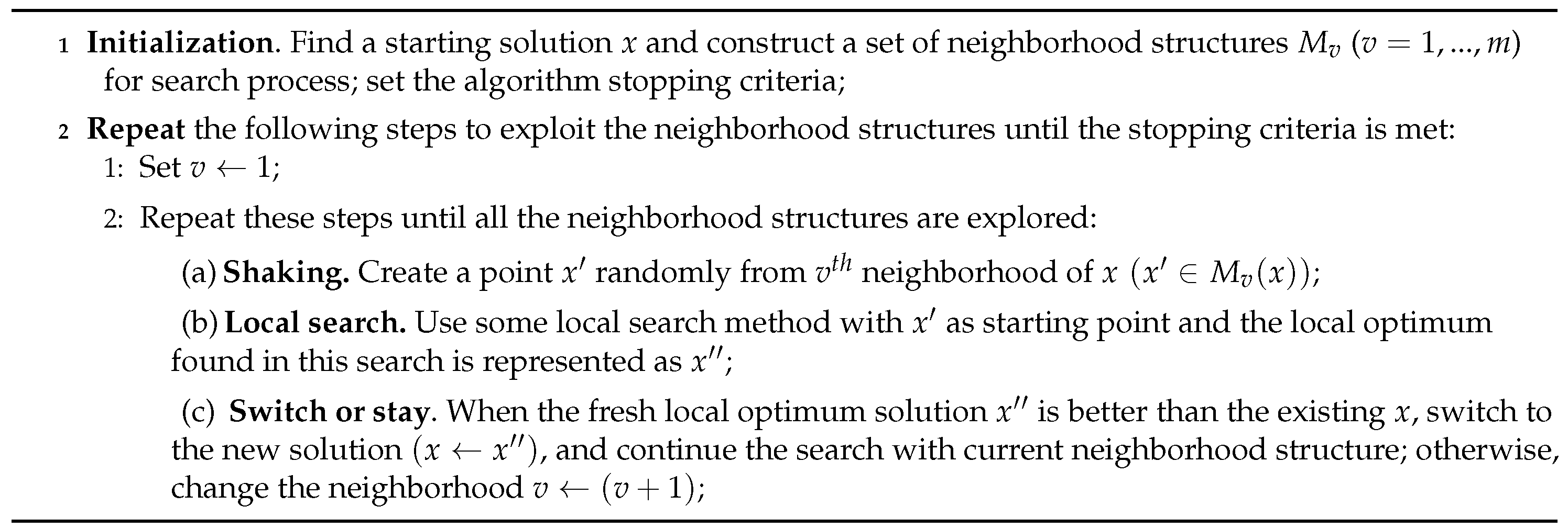
We propose two heuristic solution methods, based on the unique initial heuristic solution and VNS method. The reason for using VNS is its capability to solve such problems in an effective and innovative way. VNS was explained in detail by Hansen and Mladenović [34] as a metaheuristic for solving combinatorial and global optimization problems. The idea behind VNS is to combine the shaking procedure and a local search method in an efficient and effective way. Local search is always helpful in finding local optimal solutions but often it gets trapped in the local optima, which consumes a lot of computational time. To overcome this trap, VNS uses a solution diversification approach through shaking. The shaking procedure diversifies the search and exposes the new parts of the solution space. Starting from the initial solution x, the shaking phase is executed by randomly picking a solution from the first neighborhood structure. This is followed by local search improvement algorithm. After running the local search algorithm, a new solution $x^{″}$ is compared to the incumbent solution and acceptance decision is made. This procedure is repeated until there is no improvement or some stopping criterion is reached. Then, in a similar way, the next neighborhood structure is exposed to shaking and local search procedure. This VNS procedure is repeated until all the neighborhood structures are explored. Figure 1 further illustrates the concept of the VNS algorithm [34]. Details about initial solution, shaking and local search algorithm are given below.

4.1. Initial Heuristic Solution

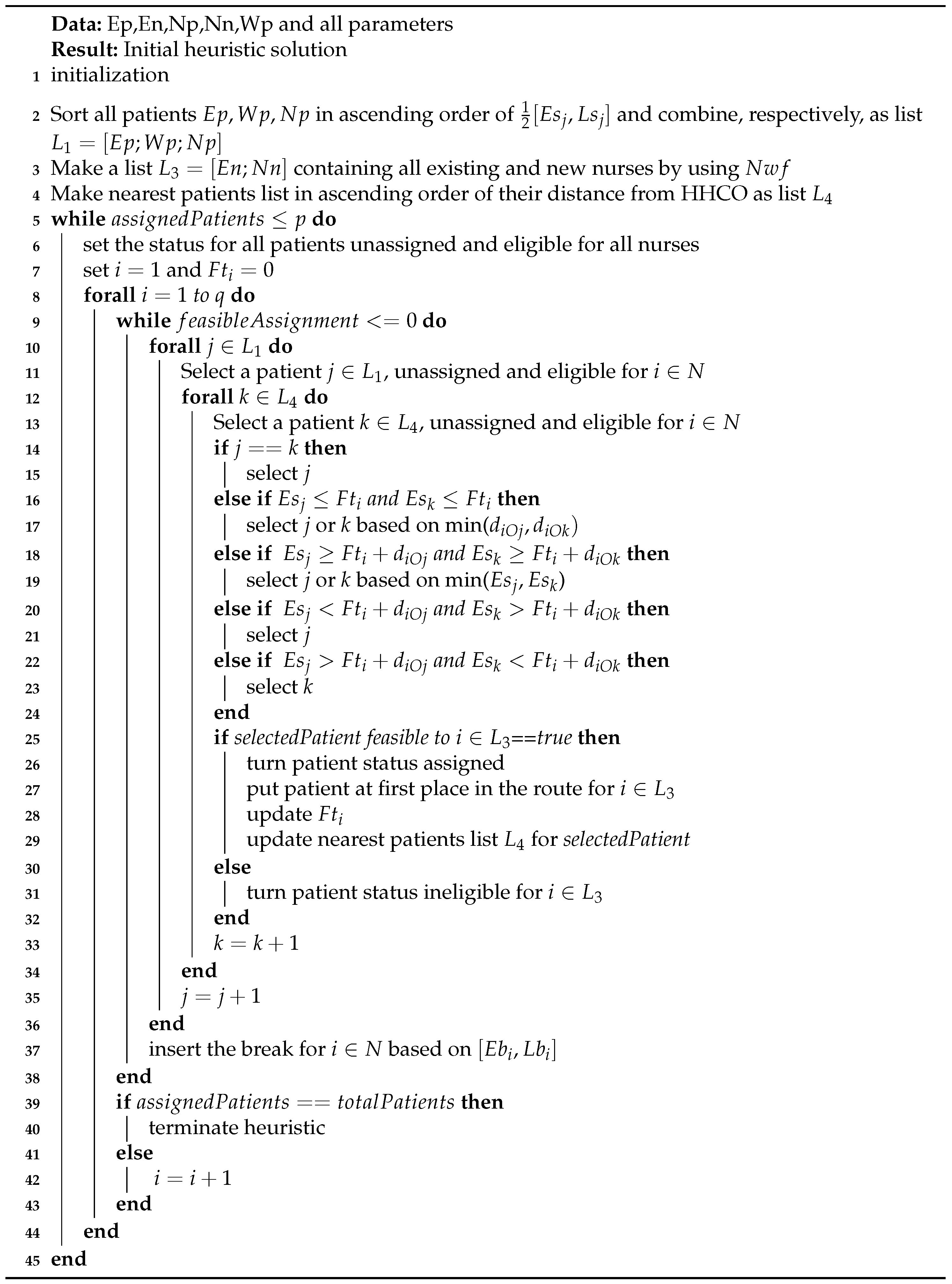
The initial heuristic solution developed here only accepts feasible solutions and guarantees the assignment of a nurse to each patient. Although the diverse nature of the nurse qualifications and patients required services are already considered by some other researchers, the diversity in terms of job status for nurses (existing, new) as well as patient selection status (existing, waiting, new) has never been explored before in the HHC problems. Therefore, it was a challenging task to keep all these aspects relevant while developing a good heuristic solution. The initial solution utilizes a nurse weighted function $\left(Nwf\right)$ to sort out existing and new nurses in ascending order as per their suitability in terms of qualification level and time windows. Appropriate weights assigned to these two parameters ensure that well qualified nurses with early time windows are assigned first. Patients are assigned to the new nurses if there is no more feasible assignment for the existing nurses. Similarly, distance and time windows of patients are simultaneously considered while assigning the most suitable patient to a nurse. Following the time windows, break activity is taken at the break node prior to departing for the next patient. The initial solution algorithm is explained in detail below and Figure 2 summarizes the concept of initial heuristic solution.

Let p be the total number of patients and q is total number of nurses.

Step 1:

Sort out all existing, waiting and new patients in ascending order of mean value of time windows $\frac{1}{2}[E{s}_j,L{s}_j]$ and make a list $L_1$ by enlisting sorted $Ep$, $Wp$ and $Np$, respectively.

Step 2:

Use nurse weighted function $\left(Nwf\right)$ to give preference to well qualified nurses with earlier time window start times. $Nwf$ takes into account two parameters to make a list $L_2$ of all existing nurses. These two parameters with their respective weights are: (a) Qualification $\left(Q_L\right)$ and (b) Time windows $(T_W$)

$Q_{Li}+T_{Wi}=1:(Q_{Li}=0.35,T_{Wi}=0.65)\forall i\in En.$

As these parameters vary for each nurse, respective weights will also vary as shown below:

(a)

$Q_{Li}=0.35$ if Qualified in all main four services.

$Q_{Li}=0.22$ if Qualified in three main services.

$Q_{Li}=0.15$ if Qualified in two main services.

(b)

Sort out all existing nurses in ascending order of mean values of time windows $\frac{1}{2}[E{r}_i,L{f}_i]$. $T_{Wi}=0.65$ and $T_{Wn}=0.65/q$, starting from first nurse in sorted list, $T_{Wi}=0.65$, then for second and third nurses, $T_{Wi+1}=T_{Wi}-T_{Wn},T_{Wi+2}=T_{Wi+1}-T_{Wn}$ and so on.

By using $Nwf$ as shown in Equation (24), update the mean value of time windows for each nurse $i\in En$ and then sort out all existing nurses in the ascending order of mean values of time windows to get the list $L_2$:

$$Nwf=\frac{1}{2}[E{r}_i,L{f}_i]+(\frac{1}{2}[E{r}_i,L{f}_i])\ast (1-(Q_{Li}+T{W}_i))\forall i\in En.$$

(24)

Step 3:

Make the third list $L_3$ by using $Nwf$ and repeating the same procedure as described in Step 2 for new nurses. Update this list by placing all the existing nurses from list $L_2$ at the start of the list $L_3$.

Step 4:

Set the status of all the patients equal to unassigned.

Step 5:

Set a nurse to patient eligibility matrix and initially set all the patients eligible to all nurses.

Step 6:

Sort out all patients in the ascending order of their distance from the HHCO as nearest patients list $L_4$.

Step 7:

Start assigning patients to nurses from first nurse $i\in L_3$ and for all the nurses set the last service finish time $F{t}_i$ equal to zero initially.

Step 8:

Starting from first patient $j\in L_1$ check the status, if this patient is eligible for nurse $i\in L_3$ and unassigned, if both yes move to Step 9; otherwise, keep searching until the right patient $j\in P$ is found.

Step 9:

Starting from first patient $k\in L_4$, check the status, if this patient is eligible for nurse $i\in L_3$ and unassigned, if both yes move to Step 10; otherwise, keep searching until the right patient $k\in P$ is found.

Step 10:

Compare these two selected patients from the lists $L_1$ and $L_4$, if patients are same ($j=k$), move to Step 12; otherwise, follow Step 11.

Step 11:

If $E{s}_j\le F{t}_i$ and $E{s}_k\le F{t}_i$, select the patient with minimum distance from HHCO, min($d_{iOj},d_{iOk})$.

If $E{s}_j\ge F{t}_i+d_{iOj}$ and $E{s}_k\ge F{t}_i+d_{iOk}$, select the patient with minimum earliest start time, min($E{s}_j,E{s}_k$).

If $E{s}_j<F{t}_i+d_{iOj}$ and $E{s}_k>F{t}_i+d_{iOk}$, select the patient $j\in L_1$ as its earliest start time allows assignment without any delay.

If $E{s}_j>F{t}_i+d_{iOj}$ and $E{s}_k<F{t}_i+d_{iOk}$, select the patient $k\in L_4$ as its earliest start time allows assignment without any delay.

Step 12:

Check the feasibility for the nurse $i\in L_3$ and selected patient, if it is feasible, assign the selected patient to the nurse $i\in L_3$ in the first place in the route and update the service finish time $F{t}_i$; otherwise, skip this patient, turn its status ineligible for nurse $i\in L_3$ and repeat Steps 8 to 12.

Step 13:

Repeat Step 6 by replacing the HHCO with the last selected feasible patient and keep assigning the patients to nurse $i\in L_3$ by repeating Steps 6 to 13.

Step 14:

During the patient assignment process to nurse $i\in L_3$, insert the break considering the break time windows $[E{b}_i,L{b}_i].$

Step 15:

If latest finish time $L{f}_i$ for nurse $i\in L_3$ is not reached, keep assigning the patients to nurse $i\in L_3$ until no more assignments are feasible; otherwise, move to the next nurse $i\in L_3$.

Step 16:

Repeat Steps 8 to 15 until all the patients are assigned.

4.2. Shaking

Shaking is a key stage in the VNS algorithm as it helps to increase the solution search space by effectively diversifying the current neighborhood structure. A solution is picked randomly from a basket of new solutions. Hence, shaking provides a direction and new solution search space is explored with the help of the local search. Neighborhood structures are the core of the VNS. We used four different neighborhood structures for our problem. These neighborhood structures are formed by cross exchange operator, 2-exchange operator, swap nurse operator and patient relocation operator.

Cross exchange operator as explained by Kindervater and Savelsbergh [35] chooses two different routes and selects a segment of nodes between two edges of each route. The length of the segment varies between one and the maximum number of nodes in a route. Then, it exchanges the selected segments between the two chosen routes, hence two new routes are formed. These two new routes are accepted on the condition of feasibility; otherwise, the same procedure is repeated first, by selecting different segments of the same routes and then choosing different routes.

2-exchange operator is similar to the cross exchange operator but with certain limitations on segment length. In our algorithm, a length of no more than two nodes is selected from each of the two selected routes. These segments are placed at a suitable place in each route and the rest of the procedure is the same as the cross exchange operator.

Swap nurse operator is different from the above-mentioned exchange operators. Instead of exchanging the segments of nodes between two routes, it swaps the two nurses with each other. In other words, the first nurse handles all the patients of the second nurse and vice versa. If feasibility check confirms both routes then, this swap move is accepted; otherwise, the same procedure is repeated by choosing two different routes.

Patient relocation operator relocates the nodes inside a route without any impact on the other routes. This neighborhood structure is implemented by removing two edges from the route then, reconnecting it by inserting the disconnected edges from the different position. If feasibility check confirms, then this route with new node positions is accepted; otherwise, this move is performed on some other edges or different positions in the same route before moving to the next route.

4.3. Local Search

VNS algorithm uses a local search method to explore the neighborhood of a new solution found through shaking, so that the solution can be improved further. In order to obtain a better local optimal solution, our algorithm uses $2-opt$ local search method introduced by Croes [36]. We use the first improvement strategy. This means that if the current solution is less costly as compared to the previous solution, the move is accepted and the search continues. This search process is repeated until the whole neighborhood of $x^{\prime }$ is explored.

The VNS algorithm used here only accepts a feasible solution; therefore, any move that gives improvement is always accepted without using any further evaluation criteria. The VNS cost function calculates all the related costs as mentioned in the objective function of MILP model and a solution is considered better if the total cost is reduced. The decision of patient acceptance, referral and sending to waiting list is made during the cost calculation step in each iteration. The decision about recruitment of a new nurse $i\in Nn$ and acceptance of new patients $j\in (Wp\cup Np)$ depends on the financial viability of the new route. Let $j\in P$ is the set of patients assigned to a nurse $i\in N$; then, nurse hiring cost, patients referral cost and waiting cost for the patients assigned to a nurse $i\in N$ can be expressed by Equations (25)–(27), respectively:

$$Cos{t}_i=C{n}_i\forall i\in N,$$

(25)

$$Cos{t}_j=\sum _{j\in P}C{p}_j{y}_j\forall j\in P,$$

(26)

$$Cos{t}_w=\sum _{s\in S}\sum _{j\in P}\sum _{w\in W}w{t}_{jw}\left(C{w}_{sw}{r}_{js}(1-p{a}_{sw})(1-p{d}_{sw})\right)\forall w\in W,\forall j\in P,\forall s\in S.$$

(27)

We compute the above-mentioned costs for each new nurse $i\in Nn$ and decide patient selection and nurse hiring by following Equation (28). If a nurse is already hired or has been assigned to an existing patient, then this nurse $i\in N$ is exempted from this process of selection. The basic concept behind this Equation (28) is that if a new nurse hiring cost is more than the patients referral cost or waiting cost for the patients assigned to this nurse, then it is rational to not accept these patients in the HHC service system. Consequently, if all the patients assigned to a nurse are referred, then that nurse route is also deleted:

$$P(z_j,y_j,w{t}_{jw})=\left\{\begin{array}{cc}{z}_j=1,\hfill & \mathrm{if}Cos{t}_j\ge C{n}_i\le Cos{t}_w,0,\mathrm{otherwise},\hfill \\ y_j=1,\hfill & \mathrm{if}C{n}_i>Cos{t}_j\le Cos{t}_w,0,\mathrm{otherwise},\hfill \\ w{t}_{jw}=1,\hfill & \mathrm{if}C{n}_i>Cos{t}_j>Cos{t}_w,0,\mathrm{otherwise}.\hfill \end{array}\right.$$

(28)

4.4. Self-Correcting VNS

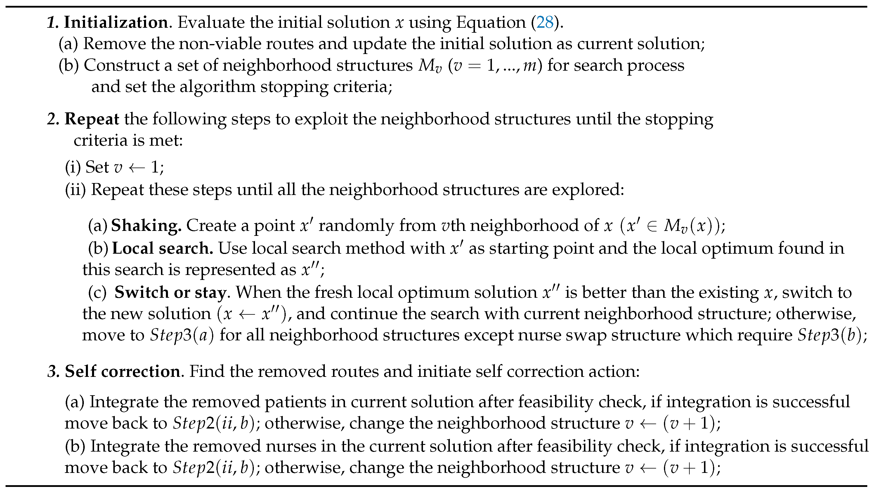
In order to reduce the computational complexity at the initial stages of VNS and better exploration of search space, we introduced the concept of a self-correcting variable neighborhood search (SCVNS). SCVNS is a self-correction and integration method combined with a variable neighborhood search method. SCVNS takes place in three steps. The first step evaluates the initial solution x before implementing the VNS. Instead of feeding all the routes determined earlier through initial solution, these routes are first evaluated with respect to associated cost. This evaluation approach uses Equation (28) to remove the routes that do not possess financial viability and reduces the size of the problem. Once the initial solution is refined, VNS is applied in the second step. The reduced size of the problem helps in better exploration of the search space in the initial stages of the VNS algorithm. The third step that performs self-correction and integration interferes with $Step2$ in two ways in the SCVNS algorithm. For all other neighborhood structures except the swap nurse operator, whenever there is no improvement in the local search, $Step3$ is activated prior to moving to the next neighborhood structure. This third step attempts to pick patients from the routes removed in the first step and integrates them in the current solution x. SCVNS identifies the removed routes and integrates the patients into the current routes as a self-correcting action, following all the compatibility requirements and feasibility check. However, for the swap nurse operator, it attempts to integrate the nurses from the removed routes by replacing them with the nurses in the current solution x and following all the compatibility requirements. When the third step interferes and successfully integrates some patients or nurses into the current solution x, the local search starts again before moving to the next neighborhood structure. As the local search method can be very time-consuming, the maximum number of iterations without improvement are restricted to five for the local search following the self-correction action. Figure 3 summarizes the concept of SCVNS.

5. Computational Experiments

The proposed heuristic algorithm and MILP model were tested on two types of randomly generated data sets, containing twenty-six cases in total. These problem instances are similar to real-life problems. The first few cases are small, typical of any new HHC firm, whereas the new patients and nurses join the existing individuals in the next instance in the same way as the new patients join the real-life HHC service system on daily basis. Data instances of type A are made in such a way that each new instance adds five new patients and two new nurses to the previous instance. The patients selected and nurses hired in the previous instance are included in the new data instance along with their start date and contract duration as the set of existing patients $Ep$ and set of existing nurses $En$, respectively. These $Ep$ and $En$ are taken from the best solution out of VNS and SCVNS. The patients sent to the waiting list are included in the next instance as a set of waiting patients $Wp$. The solution output of MILP model, VNS and SCVNS may not necessarily be the same for the patient selection and nurse recruitment decisions. Therefore, to keep uniform data instance the patients referred and the nurses not hired in the previous instance are again considered in the new instance by combining these in the set of new patients $Np$ and set of new nurses $Nn$, respectively, so that overall size of the instance remains the same for MILP model, VNS and SCVNS. Data instances of type B are similar to type A, except the difference in size. The characteristics of these data instances are given in

Table 2. Characteristics of set of instances.

Type A			Type B
Inst.	P	N	Inst.	P	N
A1	5	3	B1	20	7
A2	10	5	B2	40	14
A3	15	7	B3	60	21
A4	20	9	B4	80	28
A5	25	11	B5	100	35
A6	30	13	B6	120	42
A7	35	15	B7	140	49
A8	40	17	B8	160	56
A9	45	19	B9	180	63
A10	50	21	B10	200	70
A11	55	23	B11	220	77
A12	60	25	B12	240	84
A13	65	27	B13	260	91

, where the number of patients (P) and nurses (N) are shown against each instance.

The model formulation is implemented in optimization programming language (OPL) and solved using ILOG CPLEX 12.6 without any time limit. However, we computed the lower bounds by setting the time limit of two hours and running CPLEX in aggressive mode, whereas, the initial heuristic solution, VNS and SCVNS algorithms, were implemented in Matlab. All of the experiments were conducted on a computer with 3.20 GHz Intel Core i5 and 4 GB of RAM.

5.1. Data Generation

Data sets have been prepared through a random data generation approach. Patient locations are the random uniform coordinates in a circle with the centre of the circle at $C(25,25)$ and having a radius equal to 25 units. In this problem, HHCO and break node are located at the centre of the circle. We assume that the travel time $t_{jk}$ from location j to location k is proportional to the distance $d_{jk}$ covered by a nurse $i\in N$. Travel distances are measured with an Euclidean distance matrix.

The qualification levels of nurses range from 1 to 3 and these levels correspond to a skilled nurse in two, three and four services, respectively, out of four main services. These levels are assigned through uniform random data among the nurses considered in an instance. Similarly, service requirements are also distributed to the patients considered in the problem through uniform random data. Service time depends on the type of service required and varies between 30 and 210 min. Maximum workload for a nurse per day is no more than 420 min, excluding the time spent on breaks. Patient time windows are uniformly distributed over the whole day between 8:00 a.m. and 7:00 p.m. with a length of 180 min. Similarly, nurse time windows are uniformly distributed over the whole day between 8:00 a.m. and 10:00 p.m., with a length of 480 min, which implies that 7:00 p.m. is the latest start time for any patient, while 10:00 p.m. is the latest finish time for a nurse. Break time windows for each nurse depends on their actual time windows. In this studied problem, each nurse can start her break after 120 min following the start of work, but no later than 240 min.

The nurse hiring cost $C{n}_i$ and patient referral cost $C{p}_j$ are calculated on daily basis and depend on the qualification level of nurse and service required by the patient, respectively. Travel cost $Cd$ follows the local per kilometre fare. As the idle time cost is just a penalty imposed to reduce free time, idle time cost per minute is $Cm$, determined through several tests and equals 0.75. The idle time cost is kept less than 1 to discourage patient referral by the MILP model to decrease free time. The probability values for $p{a}_{sw}$ and $p{d}_{sw}$ are the random numbers between 0 and 1. These values are generated through uniform random data between 0 and 1 over the allowed waiting time period that is equal to four weeks. The cost of waiting $C{w}_{sw}$ for one week for each service is kept sufficiently above the patient referral cost $C{p}_j$ requiring that particular service, so that services with high chances of patient admission/departure can only host the waiting patients. Moreover, this waiting cost increases with increasing week number e.g., for second week $2^{*}C{w}_{sw}$. We set equal weights for all three sub objectives, thus ${⋌}_1={⋌}_2={⋌}_3=1$, whereas the most appropriate weights are determined for $Nwf$ parameters through a series of experiments.

5.2. Results

The results are shown in

Table 3. Numerical results comparison.

Inst.	LB	CPLEX		VNS			SCVNS
	Val.	Z	CPU	Z	Gap (%)	CPU	Z	Gap (%)	CPU
A1	904	914	1	988.4	8.14	1.91	1293.3	41.50	0.1096
A2	1749	1761.55	2	1915	8.71	28.64	2250	27.73	28.64
A3	3059	3069.7	10	3224	5.03	75	3224	5.03	75
A4	3970	4203	61,200	4396	4.59	80	4667	11.04	120
A5	3959	—	7200	5115	29.19	127	6388	61.35	73
A6	4956	—	7200	6334	27.80	1365	6334	27.80	1365
A7	5900	—	7200	7574.6	28.38	628	7574.6	28.38	628
A8	7100	—	7200	8570	20.70	985	9627	35.59	633
A9	7887	—	7200	8570	8.66	699	9147	15.98	574
A10	7900	—	7200	10,207	29.20	2328	9460	19.75	1663
A11	9240	—	7200	11,385	23.21	2520	11,660	26.19	1750
A12	10,080	—	7200	12,540	24.40	2580	12,600	25.00	1945
A13	10,790	—	7200	13,195	22.29	2700	12,725	17.93	2100
B1	3615	3620	240	4100	13.42	130	4100	13.42	130
B2	5746	—	7200	7709	34.16	1228	9491	65.18	600
B3	9720	—	7200	12,031	23.78	1311	11,380	17.08	1823
B4	12,510	—	7200	16,148	29.08	6361	17,201.73	37.50	3761
B5	15,280	—	7200	20,752	35.81	5785	20,627	34.99	6634
B6	20,040	—	7200	23,949	19.51	7516	23,946	19.49	5266
B7	21,410	—	7200	27,212	27.10	16,125	29,140	36.10	22,710
B8	26,190	—	7200	31,949	21.99	7839	33,399	27.53	14,679
B9	29,726	—	7200	36,649	23.29	13,508	35,730	20.20	24,101
B10	33,940	—	7200	39,571	16.59	25,000	36,535	7.65	22,460
B11	35,640	—	7201	44,000	23.46	25,650	43,120	20.99	23,560
B12	38,880	—	7202	45,600	17.28	27,220	44,320	13.99	24,550
B13	42,640	—	7203	51,220	20.12	28,500	51,480	20.73	26,000

and

Table 4. Patients vs. nursing staff selection and dissatisfaction costs.

Inst.	CPLEX				VNS				SCVNS
	PS	NH	NDC	PDC	PS	NH	NDC	PDC	PS	NH	NDC	PDC
A1	4	1	146.25	0	4	1	146.25	55.13	3	1	180	403.90
A2	10	2	112.50	55.13	10	2	112.50	0	8	2	168.75	888.37
A3	14	3	112.50	0	15	3	112.50	0	15	3	112.50	0
A4	20	4	78.75	73.95	20	4	112.50	0	19	4	112.50	341
A5	—	—	—	0	25	5	112.50	0	23	6	247.50	191.25
A6	—	—	—	0	30	6	112.50	0	30	6	112.50	0
A7	—	—	—	0	35	7	123.75	0	35	7	123.75	0
A8	—	—	—	0	40	8	157	0	37	8	225	942.04
A9	—	—	—	0	45	8	90	0	44	8	157.50	600.30
A10	—	—	—	0	50	10	146.25	0	49	10	258.75	55.13
A11	—	—	—	0	55	11	120	0	53	11	135.40	191.25
A12	—	—	—	0	60	13	138	0	60	11	130	0
A13	—	—	—	0	63	13	127.50	230.80	64	122	175.50	341
B1	19	4	112.50	73.95	20	4	78.75	0	20	4	78.75	0
B2	—	—	—	0	40	8	146.25	0	37	8	180	643
B3	—	—	—	0	58	13	180	396.87	57	12	213.75	1348
B4	—	—	—	0	80	16	135	0	76	16	247.50	1034.73
B5	—	—	—	0	100	21	225	0	98	20	247.50	492.90
B6	—	—	—	0	120	25	213.75	0	92	22	180	1696.30
B7	—	—	—	0	140	27	123.75	0	129	25	146.25	3718
B8	—	—	—	0	160	31	168.75	0	157	32	213.75	810.77
B9	—	—	—	0	180	36	157.50	0	178	35	180	641.89
B10	—	—	—	0	200	40	180	0	193	37	180	2452.45
B11	—	—	—	0	220	43	170.50	0	219	42	175.50	492.90
B12	—	—	—	0	240	47	220	0	240	45	123.75	0
B13	—	—	—	0	260	50	19.50	0	255	49	213.50	600.30

. Table 3 shows the performance of the MILP model using CPLEX along with the performance of VNS and SCVNS. The columns show the objective function value (Z), optimality gap (gap(%)) between the optimal solution obtained from CPLEX and heuristic solution along with computational time (cpu). The objective function value is in Hong Kong dollars (hkd), while computational time is measured in seconds. The optimality gap is computed by ${((HS-Z^{*})/Z^{*})}^{*}100$, where $Z^{*}$ is the solution obtained from CPLEX (Z), while $HS$ represents the heuristic solution (Z). CPLEX only gives optimal results for the first four instances of type A and the first instance of type B. Therefore, lower bound ($LB$) is used to compute the relative gap for all those instances where an optimal solution is not available from CPLEX. However, CPLEX delivered the $LB$ for only the first two instances of type B; therefore, we further relaxed the time window constraints to find the $LB$ for rest of the type B instances. In the case of VNS, the relative gap is less than 9%, where the optimal solution is available from CPLEX, while it is less than 30% for all instances of type A when the relative gap is computed using the lower bound. The relative gap for all instances of type B is computed using lower bound and lies between 13% and 35.81%. The relative gap for SCVNS is also calculated in the same way as VNS. The results indicate that the VNS performed better for type A instances as compared to SCVNS in terms of the optimality gap. However, SCVNS performed slightly better for type B problems in comparison to the VNS and, in some cases, the VNS and SCVNS results are similar for type A and type B. The objective values for all those instances where SCVNS performed better than VNS are shown in bold in Table 3. The poor performance of VNS for type B instances can be linked with the presence of numerous financially weak routes in the larger sized problems, as it accepted almost all the patients. Overall, the optimality gap values are good because we have computed the lower bounds, despite relaxing the time windows constraints for large sized problems as mentioned previously.

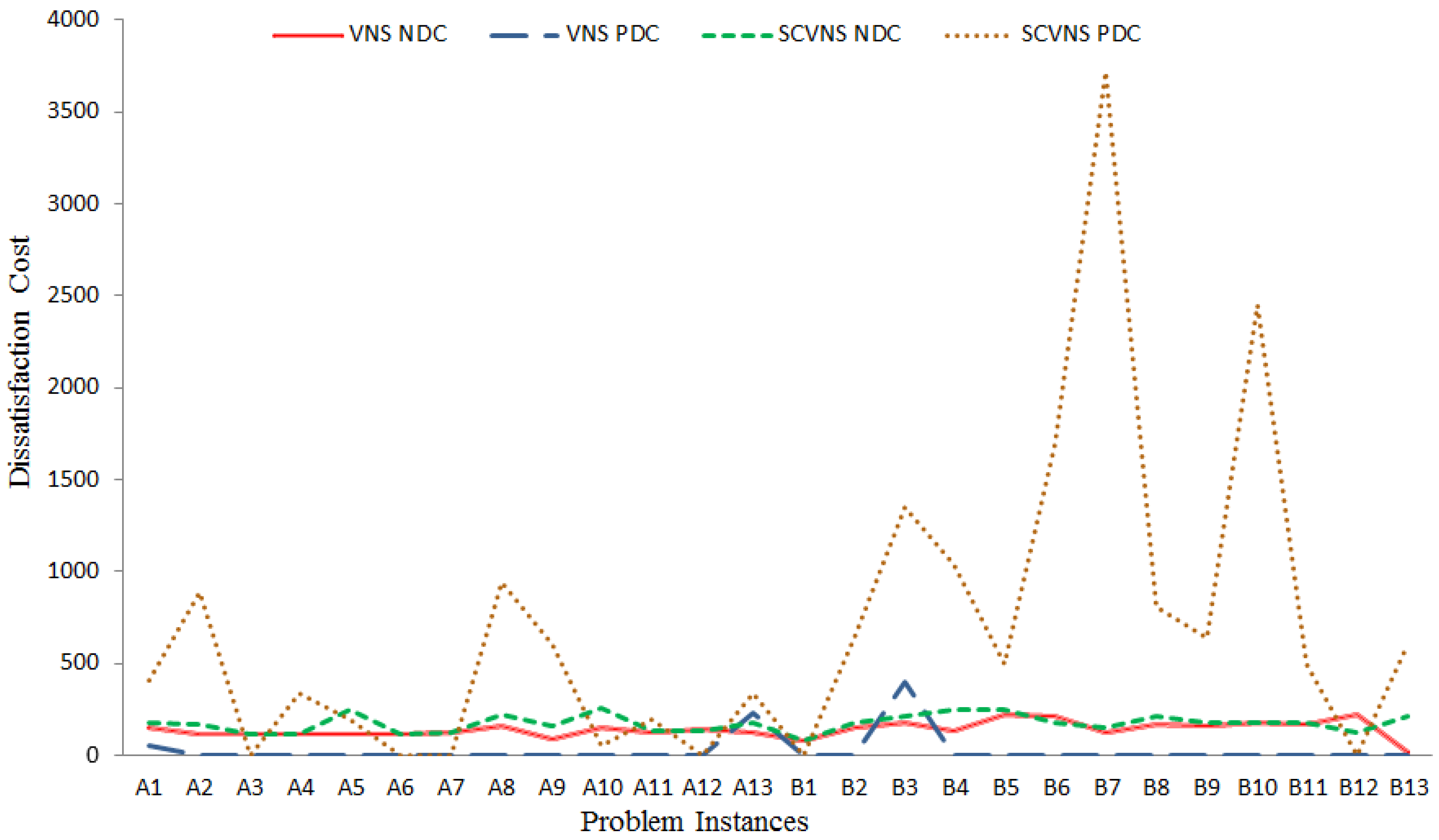
Table 4 shows the number of patients selected ($PS$), nurses hired ($NH$), nurse dissatisfaction cost ($NDC$) and patient dissatisfaction cost ($PDC$), respectively, against the CPLEX and heuristic solutions. CPLEX results available are similar as VNS; however, when comparing VNS and SCVNS, it is evident that VNS performs better than SCVNS. VNS has accepted more patients with significantly less nurse and patient dissatisfaction costs as compared to SCVNS. The average of the average number of patients assigned to each nurse in each of the instances for CPLEX, VNS and SCVNS, is 4.67, 4.95 and 4.62, respectively, as calculated from Table 4. This shows that, in every instance, VNS has not only selected more patients than CPLEX and SCVNS, but the nurse to patient assignment ratio is also higher for the VNS. The poor performance of SCVNS for the parameters described in Table 4 can be attributed to the first step of algorithm related to the evaluation of the initial solution. If a large number of financially weak routes and patients are removed in the first step, then it might not be possible to perform the self-correction and integration up to an acceptable level in Step 3 considering the large number of routes. This failure of SCVNS to integrate all the patients and routes back into the system increases patient dissatisfaction cost and nurse dissatisfaction cost, hence increasing the overall cost. This is also evident from the Figure 4, the dissatisfaction costs associated with SCVNS are higher as compared to VNS. The higher patients dissatisfaction cost is associated with the more patient referrals by SCVNS algorithm. One can conclude that VNS is slightly better than SCVNS; however, both VNS and SCVNS can be used together or alternatively for the HHC problem depending on the objective function. SCVNS could be used efficiently for the HHC planning problems where patients’ and nurses’ dissatisfaction costs are not considered important, whereas VNS is good for other cases.

HHC managers confront situations in which patients and staff join and leave the HHC system on daily basis. Consequently, the previously defined schedules, routes, and capacity calculations become invalid and there arises a genuine need to update the HHC plans following the current capacity and demand requirements. Hence, the decision-makers need those mathematical models and solution approaches that are flexible enough to incorporate such factors into the problem structure. Based on the results, it is evident that the mathematical model and proposed solution methods successfully tackled the issues considered in this study. The proposed research work enables the patient selection and nurse recruitment decisions along with the simultaneous development of assignment, scheduling, and routing plans for both existing and new entrants under the objective of cost minimization. To summarize, the modelling approach and solution method of this paper can be helpful for HHC firms to deal with the real-life scenarios and HHC managers can utilize this research for sustainable, efficient and effective HHC operations.

5.3. Sensitivity Analysis

In the earlier computational experiments, the three sub objectives were treated in the same way, with equal weights in the objective function. Sensitivity analysis was performed to study the effect of the different sub objectives on the solution and behavior of our MILP model and heuristic algorithms. First, two sub objectives were considered and then a single sub objective by assigning different weights.

Table 5. Sensitivity analysis with two sub objectives.

Inst.	${⋌}_1=0,{⋌}_2=1,{⋌}_3=1$			${⋌}_1=1,{⋌}_2=0,{⋌}_3=1$			${⋌}_1=1,{⋌}_2=1,{⋌}_3=0$
	CPLEX	VNS	Gap (%)	CPLEX	VNS	Gap (%)	CPLEX	VNS	Gap (%)
A1	201.38	292.5	45.25	767.82	842	9.66	0	0	—
A2	112.5	225	100.00	1649	1803	9.34	829	923.91	11.45
A3	123.75	125	1.00	2928	3118	6.49	1763	3224	82.87
A4	67.5	247.5	266.67	4114	4283	4.11	2993.8	4396	46.84

and

Table 6. Sensitivity analysis with single sub objective.

Inst.	${⋌}_1=1,{⋌}_2=0,{⋌}_3=0$			${⋌}_1=0,{⋌}_2=1,{⋌}_3=0$			${⋌}_1=0,{⋌}_2=0,{⋌}_3=1$
	CPLEX	VNS	Gap (%)	CPLEX	VNS	Gap (%)	CPLEX	VNS	Gap (%)
A1	0	0	—	0	0	—	0	55.3	—
A2	704	811.41	15.26	78.75	112.5	42.86	0	0	—
A3	1650	3111	88.55	112.5	112.5	0.00	0	0	—
A4	2902	4283	47.59	67	247.5	269.40	0	0	—

show the results of sensitivity analysis for two and single sub objectives, respectively. The objective function value is shown for both CPLEX and VNS in these tables. This sensitivity analysis was performed on the first four instances of type A, as CPLEX was only able to deliver optimal results for these four instances. In addition, the sensitivity analysis was restricted to VNS only, as it contains all the routes and unlike SCVNS, it does not go through the refining process by removing the financially infeasible routes of the initial solution.

In the case of pursuing the two sub objectives as shown in Table 5, when minimizing nurses’ and patients’ dissatisfaction costs, CPLEX performed better as compared to VNS. While in the case of minimization of route cost and patients’ dissatisfaction cost, the results are similar and consistent for both CPLEX and VNS, also they are not much different from the results of Table 3. However, when minimizing the route cost and nurse dissatisfaction cost, MILP delivered a low cost, but this was at the expense of selecting less patients in comparison to VNS. For both $A3$ and $A4$, four patients were referred by CPLEX, whereas VNS had a higher cost, but it accepted all the patients. Therefore, even when there is no penalty for patients’ dissatisfaction cost, the VNS algorithm shows consistency and does not start pushing referrals for more patients.

Results for minimization of single sub objective as shown in Table 6 demonstrate that, for the first instance $A1$, where no existing patients are present, both CPLEX and VNS referred the patients, as there was no penalty for patients’ dissatisfaction cost. Hence, it shows that our decision to include penalties in the MILP model for referring and sending patients to waiting list was rational. Similarly, when minimizing only patients’ dissatisfaction cost, both CPLEX and VNS accepted almost all the patients for all four instances to avoid dissatisfaction cost as shown in the last three columns of Table 6. The other results in Table 6 are somewhat similar to the above results. Thus, our heuristic algorithm delivers the sensitivity to analyse the different sub objectives of the proposed model and provides us with various insights.

The results presented in Table 3 and Table 4 along with the sensitivity analysis endorse the effectiveness of the MILP model and solution methods to accomplish the aims stated at the start of this study. Table 3 provides the cost values incurred considering each problem instance against the CPLEX and VNS based solution methods, whereas the results in Table 4 compliment the results of Table 3 by providing the actual numbers and costs against patient and nurse categories with respect to the solution methods. The MILP model successfully incorporates patient selection, staff recruitment and integration of existing and new entrants (patients, nursing staff) in the daily scheduling and routing plan while minimizing the total cost. The solutions obtained through CPLEX and VNS based heuristic methods enable an HHC firm to categorize the patients as selected (PS), referred or waiting list patients considering the existing patients (admitted and waiting list patients) and updated capacity (existing and newly recruited staff (NH)) for every planning day/period. Specifically, the sensitivity analysis shows the behavior of the model against different sub-objectives when considered jointly and individually in the HHC problem and MILP model. Thus, the HHC organizations and health care managers confronting the issues related to HHC planning, scheduling, capacity management, and dynamic demand can embrace and implement such models to smoothly plan the services and improve the sustainability and operational efficiency of the HHC services.

The HHC planning problems are highly dependent on the health care environment of a specific country and the HHC organization. Similarly, the results and effectiveness of the solution methods depend on the appropriateness of the considered issues and associated data values. The diversity of the HHC planning problems and their dependency on specific situations are also evident from the HHC literature. Therefore, to use the mathematical model developed in this study, the necessary modifications will be required by the HHC organizations. For example, the values associated with cost parameters, geographical location information, work load limits and time windows data will be changed according to the situation and regulations related to the concerned HHC organization.

6. Conclusions

In conclusion, an MILP model was developed and heuristic solution methods were suggested for the daily HHC planning problem in this paper. The model extends the HHC problem from scheduling and routing decisions to nursing staff recruitment and patient selection challenges. Existing nurse routes are optimized again by including new patients and nurses in the mathematical planning model. Long-term sustainability and flexibility for the HHC firms were the motivation behind the development of this daily HHC planning model. Furthermore, the main advantage of this model is the inbuilt flexibility in patient selection and staff hiring along with the way it handles the existing patients and nursing staff. This approach is closer to the real-life situation of home health care firms, thus having a large potential for practical application. Specifically, the integrated decision-making of our approach is suitable to new entrants in the home health care business. The results indicate that our model and heuristic algorithm have effectively addressed the problem. Moreover, the proposed solution approach achieved good results in a realistic time frame, without relaxing any of the hard constraints. In addition, the sensitivity analysis furthered our understanding of the model, providing insights about the behavior of the model against different sub objectives.

The outcome of this research is encouraging and further exploration of other aspects of this challenging problem are worthwhile. For example, it would be interesting to extend the model to include uncertainty in demands and costs as part of the problem, so that the long-term sustainability goal is ensured. One may also consider refining the solution algorithm to make it more efficient and effective by improving the initial heuristic solution and neighborhood search structures. Another very similar, but exciting and yet little explored area is hospital bed management, where bed availability is always challenging due to uncertainty regarding the length of patient stays and the dynamic pattern of patient arrivals and departures.

References

- Bard, J.F.; Shao, Y.; Qi, X.; Jarrah, A.I. The traveling therapist scheduling problem. IIE Trans. 2014, 46, 683–706. [Google Scholar] [CrossRef]
- Begur, S.V.; Miller, D.M.; Weaver, J.R. An integrated spatial DSS for scheduling and routing home-health-care nurses. Interfaces 1997, 27, 3–48. [Google Scholar] [CrossRef]
- Benzarti, E.; Sahin, E.; Dallery, Y. Operations management applied to home care services: Analysis of the districting problem. Decis. Support Syst. 2013, 55, 587–598. [Google Scholar] [CrossRef]
- Blais, M.; Lapierre, S.D.; Laporte, G. Solving a home-care districting problem in an urban setting. J. Oper. Res. Soc. 2003, 54, 1141–1147. [Google Scholar] [CrossRef]
- Carello, G.; Lanzarone, E. A cardinality-constrained robust model for the assignment problem in Home Care services. Eur. J. Oper. Res. 2014, 236, 748–762. [Google Scholar] [CrossRef]
- Perl, J.; Daskin, M.S. A Warehouse Location-Routing Problem. Transp. Res. 1985, 19B, 381–396. [Google Scholar] [CrossRef]
- Nagy, G.; Salhi, S. Nested heuristic methods for the location-routeing problem. J. Oper. Res. Soc. 1996, 47, 1166–1174. [Google Scholar] [CrossRef]
- Lee, J.H.; Moon, I.K.; Park, J.H. Multi-level supply chain network design with routing. Int. J. Prod. Res. 2010, 48, 3957–3976. [Google Scholar] [CrossRef]
- Erlenkotter, D. A comparative study of approaches to dynamic facility location problems. Eur. J. Oper. Res. 1981, 6, 133–143. [Google Scholar] [CrossRef]
- Shulman, A. An algorithm for solving dynamic capacitated plant location problems with discrete expansion sizes. Oper. Res. 1991, 39, 423–436. [Google Scholar] [CrossRef]
- Cheng, E.; Rich, L.J. A Home Health Care Routing and Scheduling Problem; Technical Report TR98-04; Department of CAAM, Rice University: Houston, TX, USA, 1998. [Google Scholar]
- Bertels, S.; Fahle, T. A hybrid setup for a hybrid scenario: Combining heuristics for the home health care problem. Comput. Oper. Res. 2006, 33, 2866–2890. [Google Scholar] [CrossRef]
- Thomsen, K. Optimization on Home Care. Master’s Thesis, Informatics and Mathematical Modelling, Technical University of Denmark, Lyngby, Denmark, 2006. [Google Scholar]
- Eveborn, P.; Flisberg, P.; Ronnqvist, M. Laps Care an operational system for staff planning of home care. Eur. J. Oper. Res. 2006, 171, 962–976. [Google Scholar] [CrossRef]
- Hertz, A.; Lahrichi, N. A patient assignment algorithm for home care services. J. Oper. Res. Soc. 2008, 60, 481–495. [Google Scholar] [CrossRef]
- Bredstrom, D.; Ronnqvist, M. Combined vehicle routing and scheduling with temporal precedence and synchronization constraints. Eur. J. Oper. Res. 2008, 191, 19–31. [Google Scholar] [CrossRef]
- An, Y.J.; Kim, Y.D.; Jeong, B.J.; Kim, S.D. Scheduling healthcare services in a home healthcare system. J. Oper. Res. Soc. 2012, 63, 1589–1599. [Google Scholar] [CrossRef]
- Trautsamwieser, A.; Hirsch, P. A Branch-Price-and-Cut approach for solving the medium-term home health care planning problem. Networks 2014, 64, 143–159. [Google Scholar] [CrossRef]
- Shao, Y.F.; Bard, J.F.; Jarrah, A.I. The therapist routing and scheduling problem. IIE Trans. 2012, 44, 868–893. [Google Scholar] [CrossRef]
- Nickel, S.; Schröder, M.; Steeg, J. Mid-term and short-term planning support for home health care services. Eur. J. Oper. Res. 2012, 219, 574–587. [Google Scholar] [CrossRef]
- Rodriguez-Verjan, C.; Augusto, V.; Xie, X. Home health-care network design: Location and configuration of home health-care centers. Oper. Res. Health Care 2017. [Google Scholar] [CrossRef]
- Bennett, A.; Erera, A. Dynamic periodic fixed appointment scheduling for home health. IIE Trans. Healthc. Syst. Eng. 2011, 1, 6–19. [Google Scholar] [CrossRef]
- Rodriguez, C.; Garaix, T.; Xie, X.; Augusto, V. Staff dimensioning in homecare services with uncertain demands. Int. J. Prod. Res. 2015, 53, 7396–7410. [Google Scholar] [CrossRef]
- Haggerty, J.L.; Reid, R.J.; Freeman, G.K.; Starfield, B.H.; Adair, C.E.; McKendry, R. Continuity of care: A multidisciplinary review. BMJ 2003, 327, 1219–1221. [Google Scholar] [CrossRef] [PubMed]
- Lanzarone, E.; Matta, A. A cost assignment policy for home care patients. Flex. Serv. Manuf. J. 2011, 24, 465–495. [Google Scholar] [CrossRef]
- Cappanera, P.; Scutellà, M.G.; Cappanera, P.; Scutellà, M.G. Joint Assignment, Scheduling, and Routing Models to Home Care Optimization: A Pattern-Based Approach. Transp. Sci. 2015, 49, 830–852. [Google Scholar] [CrossRef]
- Trautsamwieser, A.; Gronalt, M.; Hirsch, P. Securing home health care in times of natural disasters. OR Spectr. 2011, 33, 787–813. [Google Scholar] [CrossRef]
- Rasmussen, M.S.; Justesen, T.; Dohn, A.; Larsen, J. The Home Care Crew Scheduling Problem: Preference-based visit clustering and temporal dependencies. Eur. J. Oper. Res. 2012, 219, 598–610. [Google Scholar] [CrossRef]
- Mankowska, D.S.; Meisel, F.; Bierwirth, C. The home health care routing and scheduling problem with interdependent services. Health Care Manag. Sci. 2014, 17, 15–30. [Google Scholar] [CrossRef] [PubMed]
- Redjem, R.; Marcon, E. Operations management in the home care services: A heuristic for the caregivers’ routing problem. Flex. Serv. Manuf. J. 2015, 28, 280–303. [Google Scholar] [CrossRef]
- Yalçındağ, S.; Matta, A.; Şahin, E.; Shanthikumar, J.G. The patient assignment problem in home health care: Using a data-driven method to estimate the travel times of care givers. Flex. Serv. Manuf. J. 2016, 28, 304–335. [Google Scholar] [CrossRef]
- Du, G.; Liang, X.; Sun, C. Scheduling Optimization of Home Health Care Service Considering Patients’ Priorities and Time Windows. Sustainability 2017, 9, 253. [Google Scholar] [CrossRef]
- Allaoua, H.; Borne, S.; Létocart, L.; Calvo, R.W. A matheuristic approach for solving a home health care problem. Electron. Notes Discret. Math. 2013, 41, 471–478. [Google Scholar] [CrossRef]
- Hansen, P.; Mladenović, N. Variable neighborhood search. In Handbook of Metaheuristics; Glover, H.F., Kochenberger, G., Eds.; Springer: New York, NY, USA, 2003; pp. 145–184. [Google Scholar]
- Kindervater, G.; Savelsbergh, M. Vehicle routing: Handling edges exchanges. In Local Search in Combinatorial Optimization; Aarts, E.H.L., Lenstra, J.K., Eds.; Wiley: London, UK, 1997; pp. 337–360. [Google Scholar]
- Croes, G.A. A method for solving traveling salesman problems. Oper. Res. 1958, 6, 791–812. [Google Scholar] [CrossRef]
Figure 1.
Steps of the basic VNS (cf. Hansen and Mladenović [34]).