Energy Efficiency of Intensive Rice Production in Japan: An Application of Data Envelopment Analysis

Abstract

Intensive rice production has contributed to feeding the world’s growing world population, but it has also increased fossil energy consumption. This paper examines the effect of increasing the scale of rice farming on the energy efficiency of intensive rice production in Japan. A data envelopment analysis (DEA) approach is used to calculate energy efficiency scores and identify operational targets. A window analysis technique is applied to the 2005–2011 statistical data, with nine scales of rice farming, ranging from <0.5 ha to ≥15 ha. Six energy inputs (fossil fuels, electricity, chemical fertilizers, pesticides, agricultural services, and agricultural machinery) and the weight-based rice yield are selected as the DEA inputs and the DEA output, respectively. The results show that the energy efficiency scores range from 0.732 for farms of 1 ha to <2 ha, to 0.988 for farms ≥15 ha. Overall, increasing the scale of rice farming in Japan improves energy efficiency because of a great reduction in the energy consumed per unit area by agricultural machinery and agricultural services. These findings suggest that increasing the scale of farming is an effective way to enhance the energy efficiency of highly mechanized rice production in developed countries, such as Japan.

1. Introduction

Fossil fuels, which are nonrenewable resources, are indispensable to modern agriculture, contributing to impressive yields in crop production [1]. They are primarily consumed in the manufacture and operation of agricultural machinery and the production and application of chemical fertilizer [2]. Although agriculture’s share of world energy use is small, it is noteworthy that the development of energy-intensive agriculture has increased fossil fuel consumption [2].

Rice is a staple food for more than half the world’s population, with Asian regions accounting for the bulk of its production [3]. In Japan, where rice has long been the traditional staple food [4], rice production is highly mechanized compared with production in developing countries and it depends greatly on inputs produced using fossil fuels, such as chemical fertilizers [5]. About 1.63 million hectares (ha) in Japan are planted with rice, accounting for 37% of the total farmland [6]. Although Japanese rice farms have traditionally been small (the average size is 1.9–2.4 ha according to the Ministry of Agriculture, Forestry and Fisheries of Japan (MAFF) [7]), they are steadily growing in size as a result of agricultural policy reforms, including the relaxation of farmland regulations [4].

Among the numerous studies that have measured the energy efficiency of rice production (e.g., [8,9,10,11,12,13,14,15,16]), several researchers have examined whether the expansion of farm size improves the energy efficiency of rice production [17,18,19]. Nassiri and Singh [17] found that an increase in the scale of rice farming does not improve the energy efficiency of rice production in India. Similarly, Soni and Soe [19] reported that there is no statistically significant difference in energy efficiency between small-scale and large-scale rice farms in Myanmar. In contrast, Pishgar-Komleh et al. [18] showed that large-scale rice farmers in Iran have better energy indices compared with small-scale rice farmers. The focus of these studies was rice production in developing countries with relatively low levels of intensification. The effects of farm size expansion on the energy efficiency of intensive rice production in developed countries such as Japan have not been analyzed.

This paper examines the effect of increasing the scale of rice farming on the energy efficiency of intensive rice production in Japan. Agricultural policies that promote the expansion of farm size may have both positive and negative effects on various aspects of rice production. In this paper, energy efficiency indicators were used to integrate the economic and environmental aspects of an increase in the scale of rice farming. Data envelopment analysis (DEA), which is a linear programming technique for evaluating the performance of decision-making units (DMUs) [20,21], was applied to calculate the aggregate energy efficiency of rice production [9,15,17]. In contrast to traditional metrics such as the energy ratio (the energy output per unit of energy input), DEA-based energy efficiency indicators enable the identification of energy-saving targets for energy-inefficient rice farms by benchmarking them against energy-efficient farms that follow best operating practices [9,15].

2. Materials and Methods

2.1. Data Collection

Statistical data published by the MAFF in Japan are critical in developing an understanding of the fundamental characteristics of Japanese rice production. To obtain a sample of the size required for DEA calculations, 2005–2011 panel data based on scale observations of rice farming were collected from a MAFF study [7] on rice production costs in Japan. The MAFF study [7] defined the scale of rice farming by dividing rice farms into nine ranges: <0.5 ha, 0.5 to <1 ha, 1 to <2 ha, 2 to <3 ha, 3 to <5 ha, 5 to <7 ha, 7 to <10 ha, 10 to <15 ha, and ≥15 ha. In this paper, each of the nine scale ranges was regarded as constituting a rice farm (i.e., a DMU) and, therefore, nine DMUs were taken into account in the analysis. Average data for each scale range in each year were collected from the MAFF study [7]. The total sample sizes for calculating average data were 794–872 farms in 2005–2011 [7]. The sample sizes for farms in each scale range, collected for 2008–2011, were 83–94 farms in the <0.5 ha range, 121–133 in the 0.5 to <1 ha range, 139–159 in the 1 to <2 ha range, 109–117 in the 2 to <3 ha range, 131–142 in the 3 to <5 ha range, 56–68 in the 5 to <7 ha range, 56–68 in the 7 to <10 ha range, 36–44 in the 10 to <15 ha range, and 27–31 in the ≥15 ha range [7]. These data were not available for 2005–2007, as the MAFF Annual Statistics Reports do not include sample sizes for farms for each scale range [7].

Physical inputs of fossil fuels were collected to calculate the on-farm energy inputs. Due to the scarce physical data in the MAFF study [7], the production costs of inputs that were taken into account were used for calculating the off-farm energy inputs, based on an input–output approach (base year = 2005). Output data were available for the rice yield and the proceeds of rice and its by-products.

The data for 2004 and before were excluded because the classification of the scales of rice-planted areas differed from that for 2005 onward. We also omitted the data for 2012 and later, as the monetary data could not be converted into 2005 real values because of the lack of deflators for the base year (2005).

2.2. Selection of DEA Input and Output Variables

The DEA-based energy efficiency scores for rice production were calculated using the significant energy inputs and the weight-based rice yield. It is known that if a sample has a small number of DMUs relative to the total number of DEA input and output variables, then most DMUs are deemed efficient in DEA calculations [20,22,23,24]. Thus, to increase the discrimination power among DMUs, the number of DEA input and output variables was made as small as possible. It was impossible to increase the number of DMUs by extending the analysis period for the reasons mentioned above.

The candidate DEA input variables were the energy inputs of fossil fuels, electricity, seeds and seedlings, chemical fertilizers, purchased manure, pesticides, land improvement and irrigation, agricultural services, buildings, motor vehicles, and agricultural machinery. The DEA input variables used were selected on the basis of a cutoff approach; that is, an energy input variable was assumed to be significant if it contributed more than 5% of the total energy consumption of rice production [25]. Manual labor inputs, which were considered in previous studies [17,18,19], were excluded from consideration because nearly all Japanese rice production operations have been mechanized [5].

Table 1. Energy input coefficients on a net calorific value basis.

	Coefficient
Fossil fuels (GJ/L) 1
Heavy oil	0.0371
Diesel oil	0.0359
Kerosene	0.0349
Gasoline	0.0329
Motor oil	0.0382
Premixed fuel	0.0331
Production costs (GJ/million yen) 2
Fossil fuels	81.6
Electricity	472.6
Seeds and seedlings	29.2
Chemical fertilizers	79.0
Purchased manure	35.3
Pesticides	65.3
Land improvement and irrigation 3	47.3
Agricultural services 3	47.3
Buildings	46.3
Motor vehicles	42.3
Agricultural machinery	51.2

¹ 95% of gross calorific value in direct energy use [26,27]; ² Coefficients based on purchaser price for household consumables or producer price in 2005 [28]; ³ Land improvement and irrigation and agricultural services have the same coefficient because both were included in the agricultural service sector of the input–output tables [28].

lists the energy input coefficients on a net calorific value basis. The on-farm energy inputs for the six forms of fossil fuel were calculated using direct energy-use coefficients [26,27]. There was little difference in the energy input coefficients between the six forms of fossil fuel. The off-farm energy inputs were calculated by multiplying the production costs by the embodied global energy intensities, which embrace the global supply chains of Japanese products [28]. The energy input coefficient of electricity was much greater than those of other inputs.

The weight-based rice yield was used as the DEA output variable. Since by-products of rice production were excluded, the input data were allocated to rice using the share in the total proceeds of rice production from the sales of rice to calculate the energy inputs attributable to rice [29].

2.3. DEA Methodology

An input-oriented slacks-based measure of efficiency (SBM) model with variable returns to scale (VRS) was used for measuring the DEA-based energy efficiency scores for rice production. Unlike radial models, such as the Charnes–Cooper–Rhodes (CCR) model, the SBM model deals with input or output slacks directly and does not assume proportional changes in inputs or outputs [30]. Since not all inputs for rice production behave in a proportional manner, the SBM model is more appropriate than radial models such as the CCR model [30]. An input-oriented approach, i.e., one that involves setting a goal to reduce the input levels as much as possible while at least maintaining the present output levels [20], is reasonable because rice farmers have more control over the inputs responsible for energy consumption than over the outputs [31]. Given that Japanese rice farmers receive government subsidies under the rice production adjustment program [4,32], the assumption of VRS is better than that of constant returns to scale (CRS) because not all farmers operate at optimal scales [33].

In an input-oriented SBM model with VRS, if the DMUs ($j=1,\dots ,n$) have m inputs ($x_{1j},\dots ,x_{mj}$) and s outputs ($y_{1j},\dots ,y_{sj}$), the relative efficiency of each DMU_o ($o=1,\dots ,n$) to be evaluated is calculated using the following optimization model [30]:

$${\rho }_I^{*}=\underset{\mathbf{\lambda }\mathbf{,}{\mathbf{s}}^{\mathbf{-}}\mathbf{,}{\mathbf{s}}^{\mathbf{+}}}{\min }\mathbf{1}\mathbf{-}\frac{\mathbf{1}}{m}{\displaystyle \sum _{i=1}^m\frac{s_i^{-}}{x_{io}}},$$

(1)

subject to:

$$x_{io}={\displaystyle \sum _{j=1}^n{x}_{ij}{\lambda }_j+s_i^{-}}(i=1,\dots ,m),$$

(2)

$$y_{ro}={\displaystyle \sum _{j=1}^n{y}_{rj}{\lambda }_j-s_r^{+}}(r=1,\dots ,s),$$

(3)

$${\displaystyle \sum _{j=1}^n{\lambda }_j=1},$$

(4)

$${\lambda }_j\ge 0(\forall j),$$

(5)

$$s_i^{-}\ge 0(\forall i),$$

(6)

$$s_r^{+}\ge 0(\forall r),$$

(7)

where ${\rho }_I^{*}$ is SBM-input efficiency, $s_i^{-}$ is the ith input slack, $s_r^{+}$ is the rth output slack, and ${\lambda }_j$ is the jth intensity. If ${\rho }_I^{*}$ is one, a DMU_o is SBM-input efficient. When a DMU moves onto the efficient frontier, the input slacks and output slacks indicate the input excesses (potential input reductions) and the output shortfalls (potential output increases), respectively [20,30,34].

As noted, we had only nine DMUs, which corresponded to the nine scale ranges of rice farming. To address the small number of DMUs, a window analysis technique was applied to the 2005–2011 panel data, based on scale observations of rice farming [20,21]. In DEA window analysis, a DMU is dealt with as if it were a different DMU in each year [20,21]. According to Cooper et al. [20], the length of the window is calculated using:

$$p_w=\frac{k+1}{2},$$

(8)

where p_w is the length of the window and k is the number of years. As the k was seven, p_w was four years. The first, second, third, and fourth windows, respectively, included the 2005–2008, 2006–2009, 2007–2010, and 2008–2011 panel data, based on scale observations of rice farming. The DEA calculations were performed using DEA-Solver-PRO Version 10.0 [34] for the 36 DMUs (multiplying the nine DMUs by four years) in each window.

3. Results

3.1. Descriptive Statistics of the Collected Data

Table 2. Descriptive statistics of collected data on an annual mean basis (2005–2011, per year) ¹.

	Rice Farming Scale (ha Per Farm)
	<0.5	0.5 to <1	1 to <2	2 to <3	3 to <5	5 to <7	7 to <10	10 to <15	≥15
Fossil fuels (L/ha) 2
Heavy oil	0	0.1	0	0	0	0.1	0	0	0
	(0)	(0.4)	(0)	(0)	(0)	(0.4)	(0)	(0)	(0)
Diesel oil	111.4	116.4	116.7	119.4	120.1	121.2	136.0	153.9	152.8
	(11.6)	(7.9)	(1.6)	(8.7)	(7.8)	(2.4)	(6.2)	(11.4)	(9.2)
Kerosene	34.4	43.4	73.4	79.9	88.4	98.2	108.9	109.8	103.4
	(4.8)	(2.9)	(5.2)	(6.8)	(9.7)	(4.8)	(5.0)	(16.2)	(9.0)
Gasoline	94.2	88.2	75.6	72.2	67.0	59.4	60.1	64.7	44.5
	(5.0)	(4.0)	(4.5)	(7.2)	(2.9)	(7.6)	(3.2)	(5.5)	(10.2)
Motor oil	5.0	3.6	3.5	3.4	2.5	3.1	2.5	3.2	1.8
	(1.2)	(0.7)	(0.5)	(0.5)	(0.5)	(0.7)	(0.5)	(0.5)	(0.4)
Premixed fuel	19.4	15.1	8.9	4.6	4.3	2.9	2.9	2.5	0.8
	(1.6)	(1.4)	(1.3)	(1.1)	(0.8)	(0.6)	(1.1)	(1.1)	(0.7)
Production costs (thousand yen/ha) 2,3
Fossil fuels	31.8	30.7	29.9	28.7	28.5	27.9	29.6	31.7	27.9
	(3.4)	(2.6)	(2.5)	(2.8)	(3.5)	(2.6)	(3.4)	(3.6)	(3.5)
Electricity	4.4	5.5	7.3	7.2	6.5	7.3	6.5	7.3	5.4
	(0.7)	(0.8)	(0.4)	(0.7)	(0.4)	(0.6)	(0.5)	(1.1)	(0.7)
Seeds and seedlings	66.8	46.3	32.8	23.9	23.4	20.5	18.1	16.6	16.1
	(5.3)	(5.4)	(3.3)	(0.9)	(2.6)	(1.4)	(1.9)	(1.1)	(0.5)
Chemical fertilizers	88.3	81.8	75.5	75.8	71.5	76.6	69.7	63.0	64.3
	(8.8)	(7.7)	(5.4)	(7.7)	(6.5)	(5.4)	(9.3)	(5.5)	(3.8)
Purchased manure	4.1	4.1	4.6	2.4	1.9	3.4	1.3	2.4	3.3
	(1.0)	(1.0)	(0.4)	(1.1)	(1.0)	(0.8)	(1.4)	(0.8)	(1.9)
Pesticides	72.5	68.6	66.5	64.3	62.4	66.4	61.7	55.2	49.5
	(3.8)	(2.8)	(3.6)	(3.3)	(3.1)	(5.4)	(4.5)	(4.2)	(3.4)
Land improvement and irrigation	42.5	43.6	47.3	49.0	52.7	55.8	51.7	55.7	49.0
	(7.0)	(10.1)	(5.5)	(6.2)	(13.1)	(5.5)	(7.5)	(3.9)	(5.3)
Agricultural services	232.4	180.8	112.1	81.5	67.6	55.9	58.9	57.0	51.6
	(19.7)	(14.9)	(15.1)	(8.4)	(11.7)	(9.8)	(9.7)	(8.8)	(4.8)
Buildings	107.4	82.9	56.0	37.7	30.5	25.7	33.8	38.2	33.4
	(35.0)	(23.8)	(10.8)	(6.3)	(4.5)	(5.5)	(4.4)	(5.1)	(4.0)
Motor vehicles	66.2	50.5	32.8	26.1	21.0	16.8	15.9	16.3	13.2
	(14.5)	(5.5)	(3.6)	(5.5)	(1.0)	(2.5)	(2.7)	(3.5)	(1.9)
Agricultural machinery	309.5	303.1	246.4	197.1	194.1	159.3	158.0	147.9	151.4
	(61.6)	(37.9)	(12.7)	(13.8)	(13.9)	(14.3)	(25.6)	(11.9)	(7.2)
Rice yield (kg/ha)	5084	5040	5113	5231	5277	5346	5419	5380	5207
	(131)	(80)	(72)	(128)	(93)	(139)	(189)	(194)	(131)
Allocation ratio 4	0.978	0.977	0.978	0.978	0.977	0.978	0.979	0.974	0.976
	(0.002)	(0.003)	(0.004)	(0.002)	(0.003)	(0.004)	(0.005)	(0.003)	(0.006)

¹ All data were derived from MAFF [7]. Values in parentheses are standard deviations; ² Data were allocated to rice using allocation ratios; ³ Production costs were converted into real values using a price index for agricultural production materials (2005 = 100) [35]; ⁴ Allocation ratios were calculated by dividing sales of rice by total proceeds from rice production.

presents the descriptive statistics of the collected data on an annual mean basis. The data are based on a rice-planted area-based unit (per ha). The allocation ratios based on economic value (0.974–0.979 on an annual average) were used for allocating the input data to rice.

Fossil fuels that were taken into account in on-farm consumption were heavy oil (0–0.1 L/ha/year), diesel oil (111.4–153.9 L/ha/year), kerosene (34.4–109.8 L/ha/year), gasoline (44.5–94.2 L/ha/year), motor oil (1.8–5.0 L/ha/year), and premixed fuel (0.8–19.4 L/ha/year). Diesel oil had the greatest inputs across the scale ranges of rice farming, and kerosene and gasoline were the second or third greatest inputs in each scale range. As the scale of rice farming expanded, the inputs of diesel oil and kerosene increased substantially, whereas those of gasoline decreased considerably.

The production costs of rice (thousand yen/ha/year), depending on the scale of farming, were 27.9–31.8 for fossil fuels, 4.4–7.3 for electricity, 16.1–66.8 for seeds and seedlings, 63.0–88.3 for chemical fertilizers, 1.3–4.6 for purchased manure, 49.5–72.5 for pesticides, 42.5–55.8 for land improvement and irrigation, 51.6–232.4 for agricultural services, 25.7–107.4 for buildings, 13.2–66.2 for motor vehicles, and 147.9–309.5 for agricultural machinery. Many of the production costs decreased as the scale of rice farming expanded. In particular, agricultural services and agricultural machinery had the two greatest effects on cost saving when there was an increase in the scale of rice farming.

The rice yields were within the range of 5040 to 5419 kg/ha/year. Although the rice yields increased with the scale of rice farming, a downward trend was found in the data from the 7 to <10 ha range to the ≥15 ha range.

3.2. Energy Consumption

Table 3. Energy consumption of rice production on an annual mean basis (2005–2011, GJ/ha/year) ¹.

	Rice Farming Scale (ha Per Farm)
	<0.5	0.5 to <1	1 to <2	2 to <3	3 to <5	5 to <7	7 to <10	10 to <15	≥15
Fossil fuels	11.7	11.7	12.1	12.1	12.2	12.2	13.3	14.3	12.9
	(1.0)	(0.6)	(0.4)	(0.8)	(0.8)	(0.4)	(0.4)	(1.0)	(1.0)
Electricity	2.1	2.6	3.4	3.4	3.1	3.5	3.1	3.5	2.6
	(0.3)	(0.4)	(0.2)	(0.3)	(0.2)	(0.3)	(0.2)	(0.5)	(0.3)
Seeds and seedlings	2.0	1.4	1.0	0.7	0.7	0.6	0.5	0.5	0.5
	(0.15)	(0.16)	(0.10)	(0.03)	(0.08)	(0.04)	(0.06)	(0.03)	(0.01)
Chemical fertilizers	7.0	6.5	6.0	6.0	5.6	6.1	5.5	5.0	5.1
	(0.7)	(0.6)	(0.4)	(0.6)	(0.5)	(0.4)	(0.7)	(0.4)	(0.3)
Purchased manure	0.15	0.14	0.16	0.09	0.07	0.12	0.05	0.08	0.12
	(0.04)	(0.04)	(0.01)	(0.04)	(0.03)	(0.03)	(0.05)	(0.03)	(0.07)
Pesticides	4.7	4.5	4.3	4.2	4.1	4.3	4.0	3.6	3.2
	(0.2)	(0.2)	(0.2)	(0.2)	(0.2)	(0.4)	(0.3)	(0.3)	(0.2)
Land improvement and irrigation	2.0	2.1	2.2	2.3	2.5	2.6	2.4	2.6	2.3
	(0.3)	(0.5)	(0.3)	(0.3)	(0.6)	(0.3)	(0.4)	(0.2)	(0.3)
Agricultural services	11.0	8.6	5.3	3.9	3.2	2.6	2.8	2.7	2.4
	(0.9)	(0.7)	(0.7)	(0.4)	(0.6)	(0.5)	(0.5)	(0.4)	(0.2)
Buildings	5.0	3.8	2.6	1.7	1.4	1.2	1.6	1.8	1.5
	(1.6)	(1.1)	(0.5)	(0.3)	(0.2)	(0.3)	(0.2)	(0.2)	(0.2)
Motor vehicles	2.8	2.1	1.4	1.1	0.9	0.7	0.7	0.7	0.6
	(0.61)	(0.23)	(0.15)	(0.23)	(0.04)	(0.11)	(0.11)	(0.15)	(0.08)
Agricultural machinery	15.9	15.5	12.6	10.1	9.9	8.2	8.1	7.6	7.8
	(3.2)	(1.9)	(0.6)	(0.7)	(0.7)	(0.7)	(1.3)	(0.6)	(0.4)
Total	64.2	58.9	51.1	45.5	43.6	42.1	42.0	42.3	39.0
	(5.8)	(3.4)	(1.2)	(2.0)	(1.2)	(1.5)	(1.9)	(1.5)	(1.8)

¹ Energy inputs were allocated to rice using allocation ratios. Values in parentheses are standard deviations.

presents the energy consumption of rice production on an annual mean basis. The <0.5 ha range had the highest energy consumption (64.2 GJ/ha/year), whereas the ≥15 ha range had the lowest (39.0 GJ/ha/year). Thus, an increase in the scale of rice farming contributed to reducing the total energy consumption. Compared with the <0.5 ha range, the ≥15 ha range showed a decrease of 8.6 and 8.1 GJ/ha/year in the energy inputs of agricultural services and agricultural machinery, respectively.

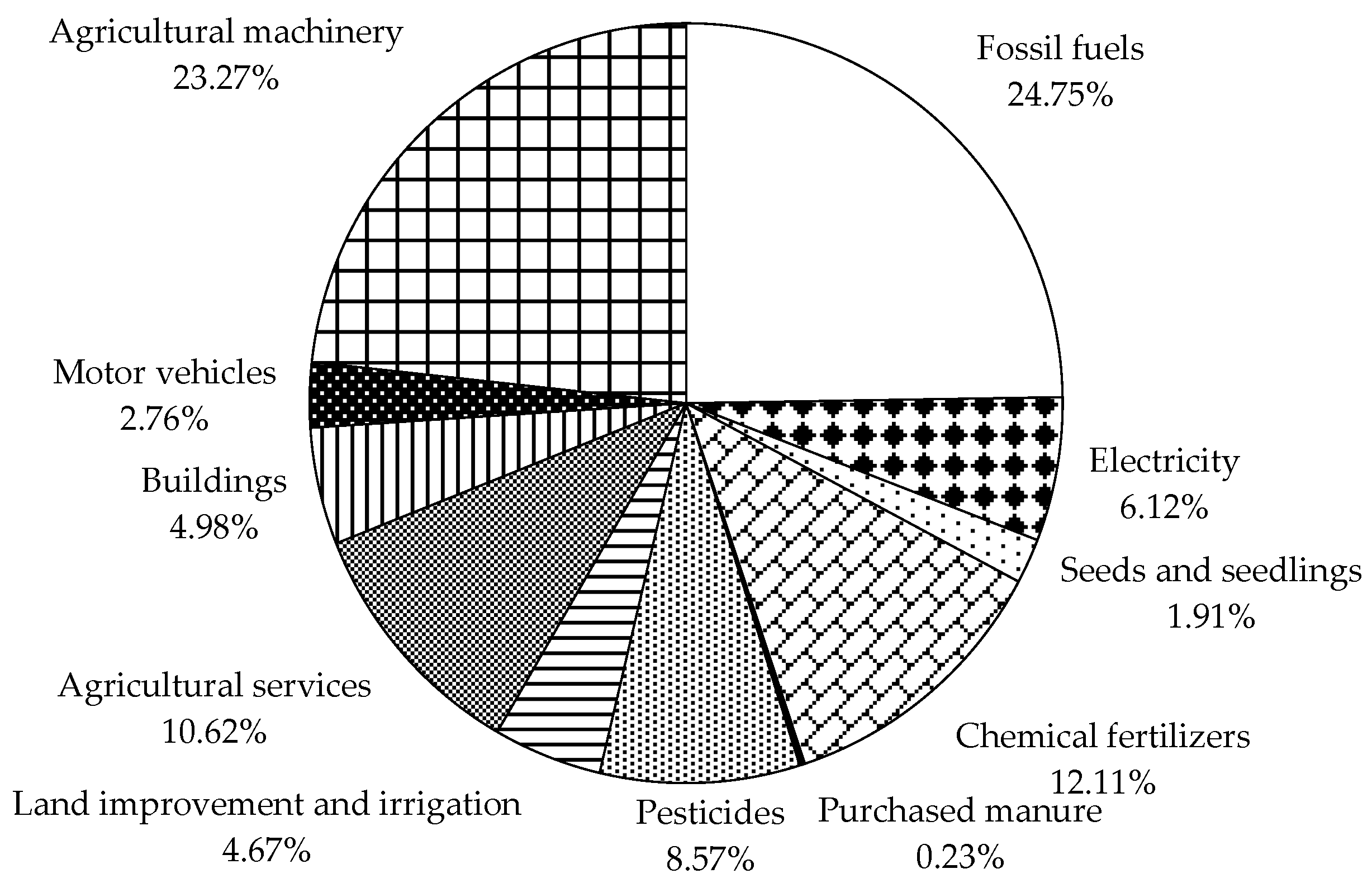
As shown in Figure 1, the contribution rates for energy consumption in rice production were, in order, fossil fuels (24.75%), agricultural machinery (23.27%), chemical fertilizers (12.11%), agricultural services (10.62%), pesticides (8.57%), and electricity (6.12%). Each of these contributors accounted for more than 5% of the total energy consumption and was thus considered to be a significant DEA input variable based on the cutoff approach.

3.3. DEA-Based Energy Efficiency Scores and Operational Targets

Table 4. Energy efficiency scores for rice production based on DEA window analysis.

	Rice Farming Scale (ha Per Farm)
	<0.5	0.5 to <1	1 to <2	2 to <3	3 to <5	5 to <7	7 to <10	10 to <15	≥15
Average for each window
2005–2008	0.99998	0.866	0.782	0.929	0.931	1	1	0.99998	0.970
2006–2009	1	0.769	0.717	0.801	0.922	0.955	0.965	0.969	0.985
2007–2010	0.903	0.677	0.717	0.794	0.891	0.907	0.929	0.940	1
2008–2011	0.818	0.657	0.714	0.789	0.882	0.871	0.891	0.926	0.996
Cumulative average	0.930	0.742	0.732	0.828	0.907	0.933	0.946	0.959	0.988

presents the energy efficiency scores for rice production based on DEA window analysis. The DEA calculations were performed using the six DEA inputs (fossil fuels, electricity, chemical fertilizers, pesticides, agricultural services, and agricultural machinery) and one DEA output (rice yield). Annual averages of energy efficiency scores were shown in each window, and cumulative averages were calculated by averaging window-based energy efficiency scores. From the perspective of cumulative averages, the energy efficiency scores ranged from 0.732 for the 1 to <2 ha range to 0.988 for the ≥15 ha range. The energy efficiency scores increased with the scale of rice farming, although the <0.5 ha range, the smallest scale of rice farm considered, had a relatively high score (0.930).

Table 5. Operational targets for rice production based on cumulative averages from DEA window analysis.

	Rice Farming Scale (ha Per Farm)
	<0.5	0.5 to <1	1 to <2	2 to <3	3 to <5	5 to <7	7 to <10	10 to <15	≥15
Fossil fuels
Potential reduction (GJ/ha)	0.153	0.267	0.329	0.109	0.024	0.059	0.161	0.387	0.060
Potential reduction rate (%)	1.3	2.3	2.7	0.9	0.2	0.5	1.2	2.7	0.5
Electricity
Potential reduction (GJ/ha)	0.045	0.349	1.014	0.746	0.350	0.421	0.214	0.228	0.032
Potential reduction rate (%)	2.2	13.1	29.2	22.1	11.3	12.5	7.1	6.7	1.3
Chemical fertilizers
Potential reduction (GJ/ha)	0.419	1.091	0.868	0.778	0.583	0.527	0.563	0.186	0.073
Potential reduction rate (%)	6.0	16.9	14.5	13.0	10.3	8.6	10.2	3.7	1.4
Pesticides
Potential reduction (GJ/ha)	0.369	1.133	1.180	0.844	0.523	0.399	0.351	0.245	0.048
Potential reduction rate (%)	7.9	25.6	27.6	20.4	13.0	9.4	9.0	7.0	1.5
Agricultural services
Potential reduction (GJ/ha)	1.525	4.603	2.662	1.249	0.283	0.206	0.073	0.114	0.080
Potential reduction rate (%)	14.2	54.5	51.7	31.9	9.1	7.5	2.7	4.4	3.4
Agricultural machinery
Potential reduction (GJ/ha)	2.259	7.032	4.582	1.702	1.361	0.296	0.379	0.052	0.005
Potential reduction rate (%)	14.1	44.6	36.2	17.0	13.6	3.6	4.7	0.7	0.1
Rice yield
Potential increase (kg/ha)	0.02	26.1	36.2	22.3	0	0	3.6	10.1	10.8
Potential increase rate (%)	0.0004	0.5	0.7	0.4	0	0	0.1	0.2	0.2

presents the operational targets for rice production based on cumulative averages from the DEA window analysis. The potential reductions for the DEA inputs and the potential increases for rice yields indicate the variations required for a DMU to become efficient [20,30,34]. The 1 to <2 ha and 0.5 to <1 ha ranges, which had the two lowest energy efficiency scores (0.732–0.742 on a cumulative average basis; refer to Table 4), had larger potential reductions for the DEA inputs, especially for agricultural machinery (4.582–7.032 GJ/ha) and agricultural services (2.662–4.603 GJ/ha), and greater potential increases (26.1–36.2 kg/ha) for rice yield than the other ranges. In these ranges, the potential reduction rates for agricultural machinery (36.2–44.6%) and agricultural services (51.7–54.5%) were very high, whereas the potential increase rates (0.5–0.7%) for rice yield were extremely low.

4. Discussion

4.1. Findings and Implications

The primary reason that DEA-based energy efficiency scores increased with the scale of rice farming in Japan was that the indirect energy inputs per hectare for agricultural machinery and agricultural services decreased greatly with scale. Thus, both of these inputs are key operational reduction targets for improving DEA-based energy efficiency indicators. In this paper, the values of the off-farm energy inputs were calculated using the energy coefficients per unit of cost [28]. Therefore, a great reduction in the costs per hectare of agricultural machinery and agricultural services results in a great reduction in these energy inputs. Although large-scale rice farmers purchase larger and more expensive agricultural machines than do small-scale farmers [7], their cost per hectare is less, reflecting economies of size or, in other words, the ability of a farm to lower its costs of production by expanding size [36]. Moreover, the greater investment in agricultural machinery by these larger farms contributes to a greater decrease in the cost of agricultural services per hectare, by considerably reducing dependence on contractors for services such as harvesting [7].

In contrast, fossil fuels, electricity, chemical fertilizers, and pesticides were not found to be important as operational reduction targets. The primary reason that the energy potential reductions per hectare for fossil fuels and electricity are small is that their energy inputs per hectare increase with the scale of rice farming. Large-scale rice farmers who do much of the work themselves have much greater inputs per hectare for diesel oil for field work and kerosene for grain drying than do small-scale farmers, who are highly dependent on contractors [7]. They also require more electricity inputs per hectare for grain dryers and rice hullers during postharvest operations than do the small-scale farmers [7].

Unlike fossil fuels and electricity, the energy inputs per hectare for chemical fertilizers and pesticides decrease as the scale of rice farming increases. In Japan, large-scale rice farms have a higher adoption rate of environmentally friendly farming practices compared with small-scale farmers, resulting in reduced use of chemical fertilizers and pesticides [4]. However, little difference was found between large- and small-scale rice farms in the energy inputs per hectare for chemical fertilizers and pesticides. Thus, their energy potential reductions per hectare are small.

The input-oriented SBM model with VRS used in the DEA calculations yielded the potential increases for the DEA output, in addition to the potential reductions for the DEA inputs [30,34]. The potential increases for the rice yield were zero or extremely small because an input-oriented assumption was made in the DEA calculations [20], and there is little difference in rice yields for the different scale ranges of rice farming, compared with the DEA inputs, such as agricultural machinery and agricultural services.

Our results demonstrate the advantages that are gained by increasing the scale of rice farming. This is especially important in improving the energy efficiency of highly-mechanized rice production in developed countries, such as Japan. However, these results differ from those found in developing countries, where the advantages of scale are not an effective way to enhance the energy efficiency of low-level mechanized rice production because the indirect energy input of agricultural machinery accounts for only a very small percentage of the total energy consumption of rice production [17,18,19].

4.2. Lack of Discrimination Power for the <0.5 ha Range

Since the <0.5 ha range has relatively large energy inputs and low rice yields, its DEA-based energy efficiency scores should be small. However, given that the DEA-based energy efficiency scores are in the range of 0.732 to 0.988 on a cumulative average basis, the <0.5 ha range has a very high score (0.930).

One possible reason for the poor discrimination within this range of rice farming is the relatively few DMUs compared with the number of DEA input and output variables [20,22,23,24]. Several rules of thumb have been proposed for the number of DMUs required for achieving a reasonable level of discrimination, e.g., $2m\times s$ [23] and $3(m+s)$ [20], where m and s are the number of DEA inputs and outputs, respectively. Since 36 DMUs (multiplying nine DMUs by four years) with six inputs and one output were included in each window, the DEA calculations satisfied both rules. Thus, in this case, a lack of DMUs was not a major reason for the deficient discrimination power for the <0.5 ha range.

Another possible reason is the assumption of VRS. If a subset of DMUs operates at a very different scale compared with the remaining DMUs, they will be classified as efficient in DEA calculations with VRS [22,24]. Further, if there are no inherent scale effects, small and large DMUs will be overrated in DEA calculations with VRS [23]. This possibility was investigated by comparing the DEA-based energy efficiency scores calculated under the assumption of VRS with those calculated under the assumption of CRS. With CRS, the DEA-based energy efficiency scores on a cumulative average basis ranged from 0.714 for the 1 to <2 ha range to 0.978 for the ≥15 ha range, with a score of 0.910 for the <0.5 ha range. These results are very similar to the DEA-based energy efficiency scores calculated with VRS. This indicates that the assumption of VRS was not a major reason for the lack of discrimination power for the <0.5 ha range.

Although the data collection period (2005–2011) could not be extended because of the lack of deflators for the base year (2005), if the data from 2012 were included in the analysis, the discrimination might be improved for the <0.5 ha range. In the DEA window analysis, the <0.5 ha range for 2005–2009 was determined to be efficient or nearly efficient, whereas that for 2010–2011 was determined to be very inefficient (0.613–0.658).

5. Conclusions

DEA-based energy efficiency indicators for intensive rice production in Japan were evaluated in accordance with the scale of rice farming. DEA window analysis was applied to panel data based on scale observations of rice farming that were collected from MAFF data for 2005–2011. Six DEA inputs (fossil fuels, electricity, chemical fertilizers, pesticides, agricultural services, and agricultural machinery) and one DEA output (rice yield) were used in the DEA calculations, which were based on an input-oriented SBM model with VRS.

The results showed that, overall, increasing the scale of rice farming improves the energy efficiency of intensive rice production. This is because an increase in the scale of rice farming that involves greater agricultural machinery investment greatly reduces the energy inputs per unit area for both agricultural machinery and agricultural services. The findings suggest that the advantages that result from an increase in the scale of farming are especially effective in enhancing the energy efficiency of highly-mechanized rice production in developed countries such as Japan. However, energy efficiency improvements based on these advantages of scale would not necessarily be realized for low-level mechanized rice production in developing countries.

To develop larger rice farms, Japanese agricultural policies have been reformed by applying the important payment programs to business-oriented farmers, in addition to relaxing the farmland regulations [4,32]. Further, because the rice production adjustment program prevents competitiveness by increasing rice production costs and muting market signals [4,32], its abolishment will also contribute to building larger rice farms. These agricultural policy reforms should promote energy-efficient rice production in Japan, resulting in larger-scale farming.

In this paper, to address the small number of DMUs, a window analysis technique was applied to the panel data based on scale observations of rice farming. Further studies are needed to better understand the time trends regarding the energy efficiency of Japanese rice farms.

References

- Pimentel, D.; Hurd, L.E.; Bellotti, A.C.; Forster, M.J.; Oka, I.N.; Sholes, O.D.; Whitman, R.J. Food production and the energy crisis. Science 1973, 182, 443–449. [Google Scholar] [CrossRef] [PubMed]
- Faidley, L.W. Energy and agriculture. In Energy in Farm Production; Fluck, R.C., Ed.; Elsevier: Amsterdam, The Netherlands, 1992; pp. 1–12. [Google Scholar]
- Food and Agriculture Organization of the United Nations (FAO). FAO Statistical Yearbook 2014: Asia and the Pacific. Food and Agriculture; FAO Regional Office for Asia and the Pacific: Bangkok, Thailand, 2014. [Google Scholar]
- Organisation for Economic Co-operation and Development (OECD). Evaluation of Agricultural Policy Reforms in Japan; OECD Publishing: Paris, France, 2009. [Google Scholar]
- Barker, R.; Herdt, R.W. The Rice Economy of Asia; Resources for the Future: Washington, DC, USA, 1985. [Google Scholar]
- Ministry of Agriculture, Forestry and Fisheries of Japan (MAFF). Statistics on Cultivated Land and Planted Area (2011). Available online: http://www.e-stat.go.jp/SG1/estat/List.do?lid=000001087149 (accessed on 6 September 2016). (In Japanese)
- Ministry of Agriculture, Forestry and Fisheries of Japan (MAFF). Production Cost of Rice, Wheat, and Barley (2005–2011). Available online: http://www.maff.go.jp/j/tokei/kouhyou/noukei/seisanhi_nousan/ (accessed on 2 September 2015). (In Japanese)
- AghaAlikhani, M.; Kazemi-Poshtmasari, H.; Habibzadeh, F. Energy use pattern in rice production: A case study from Mazandaran province, Iran. Energy Convers. Manag. 2013, 69, 157–162. [Google Scholar] [CrossRef]
- Chauhan, N.S.; Mohapatra, P.K.J.; Pandey, K.P. Improving energy productivity in paddy production through benchmarking: An application of data envelopment analysis. Energy Convers. Manag. 2006, 47, 1063–1085. [Google Scholar] [CrossRef]
- Eskandari, H.; Attar, S. Energy comparison of two rice cultivation systems. Renew. Sustain. Energy Rev. 2015, 42, 666–671. [Google Scholar] [CrossRef]
- Hafeez, M.; Bundschuh, J.; Mushtaq, S. Exploring synergies and tradeoffs: Energy, water, and economic implications of water reuse in rice-based irrigation systems. Appl. Energy 2014, 114, 889–900. [Google Scholar] [CrossRef] [Green Version]
- Kazemi, H.; Kamkar, B.; Lakzaei, S.; Badsar, M.; Shahbyki, M. Energy flow analysis for rice production in different geographical regions of Iran. Energy 2015, 84, 390–396. [Google Scholar] [CrossRef]
- Mandal, S.; Roy, S.; Das, A.; Ramkrushna, G.I.; Lal, R.; Verma, B.C.; Kumar, A.; Singh, R.K.; Layek, J. Energy efficiency and economics of rice cultivation systems under subtropical Eastern Himalaya. Energy Sustain. Dev. 2015, 28, 115–121. [Google Scholar] [CrossRef]
- Mushtaq, S.; Maraseni, T.N.; Maroulis, J.; Hafeez, M. Energy and water tradeoffs in enhancing food security: A selective international assessment. Energy Policy 2009, 37, 3635–3644. [Google Scholar] [CrossRef] [Green Version]
- Nabavi-Pelesaraei, A.; Abdi, R.; Rafiee, S.; Taromi, K. Applying data envelopment analysis approach to improve energy efficiency and reduce greenhouse gas emission of rice production. Eng. Agric. Environ. Food 2014, 7, 155–162. [Google Scholar] [CrossRef]
- Rahman, S.; Barmon, B.K. Exploring the potential to improve energy saving and energy efficiency using fertilizer deep placement strategy in modern rice production in Bangladesh. Energy Effic. 2015, 8, 1241–1250. [Google Scholar] [CrossRef]
- Nassiri, S.M.; Singh, S. Study on energy use efficiency for paddy crop using data envelopment analysis (DEA) technique. Appl. Energy 2009, 86, 1320–1325. [Google Scholar] [CrossRef]
- Pishgar-Komleh, S.H.; Sefeedpari, P.; Rafiee, S. Energy and economic analysis of rice production under different farm levels in Guilan province of Iran. Energy 2011, 36, 5824–5831. [Google Scholar] [CrossRef]
- Soni, P.; Soe, M.N. Energy balance and energy economic analyses of rice production systems in Ayeyarwaddy Region of Myanmar. Energy Effic. 2016, 9, 223–237. [Google Scholar] [CrossRef]
- Cooper, W.W.; Seiford, L.M.; Tone, K. Data Envelopment Analysis: A Comprehensive Text with Models, Applications, References and DEA-Solver Software, 2nd ed.; Springer: New York, NY, USA, 2007. [Google Scholar]
- Cooper, W.W.; Seiford, L.M.; Zhu, J. Data envelopment analysis: History, models, and interpretations. In Handbook on Data Envelopment Analysis, 2nd ed.; Cooper, W.W., Seiford, L.M., Zhu, J., Eds.; Springer: New York, NY, USA, 2011; pp. 1–39. [Google Scholar]
- Cooper, W.W.; Ruiz, J.L.; Sirvent, I. Choices and uses of DEA weights. In Handbook on Data Envelopment Analysis, 2nd ed.; Cooper, W.W., Seiford, L.M., Zhu, J., Eds.; Springer: New York, NY, USA, 2011; pp. 93–126. [Google Scholar]
- Dyson, R.G.; Allen, R.; Camanho, A.S.; Podinovski, V.V.; Sarrico, C.S.; Shale, E.A. Pitfalls and protocols in DEA. Eur. J. Oper. Res. 2001, 132, 245–259. [Google Scholar] [CrossRef]
- Podinovski, V.V.; Thanassoulis, E. Improving discrimination in data envelopment analysis: Some practical suggestions. J. Prod. Anal. 2007, 28, 117–126. [Google Scholar] [CrossRef]
- Raynolds, M.; Fraser, R.; Checkel, D. The relative mass-energy-economic (RMEE) method for system boundary selection. Part 1: A means to systematically and quantitatively select LCA boundaries. Int. J. Life Cycle Assess. 2000, 5, 37–46. [Google Scholar] [CrossRef]
- Greenhouse Gas Inventory Office of Japan (GIO) (Ed.) National Greenhouse Gas Inventory Report of Japan (2015); National Institute for Environmental Studies: Tsukuba, Japan, 2015.
- International Energy Agency (IEA). Energy Statistics Manual; IEA Publications: Paris, France, 2005. [Google Scholar]
- Nansai, K.; Kondo, Y.; Kagawa, S.; Suh, S.; Nakajima, K.; Inaba, R.; Tohno, S. Estimates of embodied global energy and air-emission intensities of Japanese products for building a Japanese input–output life cycle assessment database with a global system boundary. Environ. Sci. Technol. 2012, 46, 9146–9154. [Google Scholar] [CrossRef] [PubMed]
- Guinée, J.B. (Ed.) Handbook on Life Cycle Assessment: Operational Guide to the ISO Standards; Kluwer Academic Publishers: Dordrecht, The Netherlands, 2002. [Google Scholar]
- Tone, K. Slacks-based measure of efficiency. In Handbook on Data Envelopment Analysis, 2nd ed.; Cooper, W.W., Seiford, L.M., Zhu, J., Eds.; Springer: New York, NY, USA, 2011; pp. 195–209. [Google Scholar]
- Galanopoulos, K.; Aggelopoulos, S.; Kamenidou, I.; Mattas, K. Assessing the effects of managerial and production practices on the efficiency of commercial pig farming. Agric. Syst. 2006, 88, 125–141. [Google Scholar] [CrossRef]
- Ministry of Agriculture, Forestry and Fisheries of Japan (MAFF). Summary of Farming Income Stabilization Measures in 2016. Available online: http://www.maff.go.jp/j/kobetu_ninaite/keiei/pdf/28pamph_all.pdf (accessed on 31 October 2016). (In Japanese)
- Lozano, S.; Iribarren, D.; Moreira, M.T.; Feijoo, G. The link between operational efficiency and environmental impacts: A joint application of life cycle assessment and data envelopment analysis. Sci. Total Environ. 2009, 407, 1744–1754. [Google Scholar] [CrossRef] [PubMed]
- SaiTech. User’s Guide to DEA-Solver-PRO (Professional Version 10.0); SaiTech: Holmdel, NJ, USA, 2013. [Google Scholar]
- Ministry of Agriculture, Forestry and Fisheries of Japan (MAFF). Statistics on Commodity Prices in Agriculture (2011). Available online: http://www.e-stat.go.jp/SG1/estat/List.do?lid=000001102155 (accessed on 5 October 2015). (In Japanese)
- Duffy, M. Economies of size in production agriculture. J. Hunger Environ. Nutr. 2009, 4, 375–392. [Google Scholar] [CrossRef] [PubMed]
Figure 1.
Contributors to the energy consumption of rice production based on a weighted average for all scale ranges of rice farming in 2005–2011. The weighted average was weighted with respect to the average values of sample sizes for each scale range in 2008–2011 [7].