Physical Layer Network Coding Based on Integer Forcing Precoded Compute and Forward

Abstract

In this paper, we address the implementation of physical layer network coding (PNC) based on compute and forward (CF) in relay networks. It is known that the maximum achievable rates in CF-based transmission is limited due to the channel approximations at the relay. In this work, we propose the integer forcing precoder (IFP), which bypasses this maximum rate achievability limitation. Our precoder requires channel state information (CSI) at the transmitter, but only that of the channel between the transmitter and the relay, which is a feasible assumption. The overall contributions of this paper are three-fold. Firstly, we propose an implementation of CF using IFP and prove that this implementation achieves higher rates as compared to traditional relaying schemes. Further, the probability of error from the proposed scheme is shown to have up to 2 dB of gain over the existent lattice network coding-based implementation of CF. Secondly, we analyze the two phases of transmission in the CF scheme, thereby characterizing the end-to-end behavior of the CF and not only one-phase behavior, as in previous proposals. Finally, we develop decoders for both the relay and the destination. We use a generalization of Bezout’s theorem to justify the construction of these decoders. Further, we make an analytical derivation of the end-to-end probability of error for cubic lattices using the proposed scheme.

1. Introduction

Modern wireless vehicular networks are highly dynamic, and the connectivity of such networks is heavily dependent on key techniques, like relaying. Relaying is an important strategy in wireless vehicular networking, and therefore, it has received much attention in recent years. Physical layer network coding (PNC) is a new paradigm of relaying [1] in which intermediate nodes in a wireless network, instead of decoding individual symbols from the received signals, decode a linear combination of symbols and send them to the destination node. Upon obtaining sufficient combinations, the destination node can decode the original signals.

In [2], Nazer and Gastpar proposed a novel strategy of generalized relaying, called compute and forward (CF), which enables the relays in any Gaussian wireless network to decode linear equations of the transmitted symbols with integer coefficients, using the noisy linear combinations provided by the channel. The linear equations are transmitted to the destination, and upon receiving sufficient linear equations, the destination can decode the desired symbols. The key point in this strategy is the use of nested lattice codes for encoding the original messages. Nested lattice codes satisfy the property that a linear combination of codewords gives another codeword. Further, information theoretical tools are used in [2] to obtain the achievable rate regions.

An algebraic approach to implement CF has been introduced in [3]. In this work, the authors have related the approach introduced by Nazer and Gastpar to the fundamental theorem of finitely generated modules over the principal ideal domain (PID). Consequently, the isomorphism between the message space and the physical signal space (equivalently between the link layer and physical layer) is identified using module theory. Furthermore, the authors identify the lattices and lattice partitions, which can be utilized to implement CF in finite dimensions. The authors show that the union bound estimate for the probability of decoding a linear equation at the relay node is limited by the gap between the channel gain and the integer approximation.

In [4], Niesen and Whiting have analyzed the asymptotic behavior of CF and pointed to a fundamental limitation. They have shown that the degrees of freedom (DoF) achievable by the lattice-based implementation of CF is at most two, when the channel gains are irrational. This is due to the gap between the natural channel gains and the integer coefficient of the linear combination in coherence to the observation in [3]. Further, it is proved that this limitation is not inherent to the fundamental concept of CF, but is due to the lattice-based implementation of CF. In addition, it has also been shown in [4] that the maximum DoF can be achieved by CF when channel state information (CSI) is available at the transmitter.

Another recent work in [5] studies the practical aspects of CF. Specifically, the decoding techniques are studied, and it is shown that the additional noise created due to the non-integer channel coefficients makes the effective noise non-Gaussian and increases the complexity of Maximum likelihood decoding in CF.

The study of CF has attracted the attention of the research community, and a wide body of work is available in the literature. Interested readers can refer to an extensive survey of the recent developments in CF in [6]. Different implementations of CF have also been proposed. The selection of integer coefficients of linear combination at the relay has been studied in [7], where the authors provide a scheme to choose sub-optimal integer coefficients without using CSI at the relay. Further, in [8,9], precoding-postcoding techniques have been studied in order to minimize the effects of the non-integer channel penalty in some scenarios, particularly, using the spatial orientation of signals.

Motivated by these results, in this paper, we aim to remove the decoding limitations of the previous proposals, focusing on the physical layer. Particularly, the existing limitation in performance of CF is due to the approximation of the channel by an integer contributing to additional self-noise apart from receiver noise. In this paper, we propose a precoder, which removes the self-noise completely and, therefore, improves the performance of CF. Further, in most of the existent works, the performance of CF is studied at the relay node, assuming the transmission from relay-to-destination to be perfect point-to-point transmission. As an extension of our work in [10], we consider a noisy transmission from relay-to-destination and analyze the end-to-end performance of CF.

1.1. Main Contributions

The main contributions of this paper are as follows:

• We propose a novel precoding technique to implement physical layer network coding using CF. Our precoder design is based on integer forcing and allows bypassing the self-noise limitation of existing formulations, thus providing higher achievable rates than existent relaying schemes.
• We developed a decoder for relays of CF and characterized it using the generalization of Bezout’s theorem. We also made an analytical derivation of the end-to-end probability of error for cubic lattices.
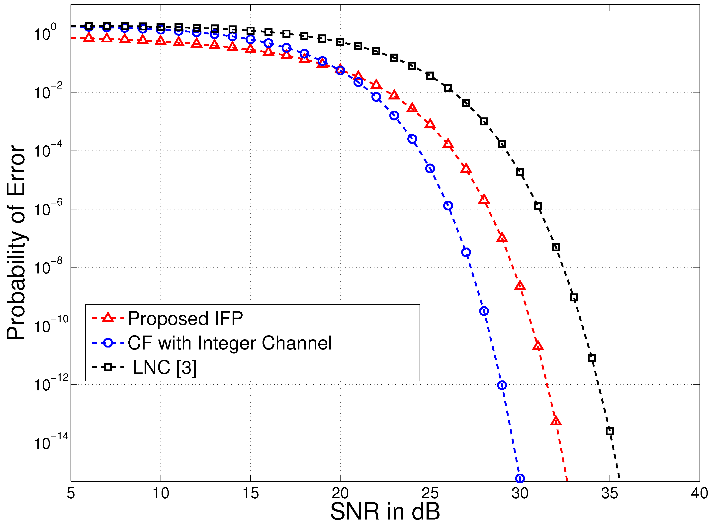
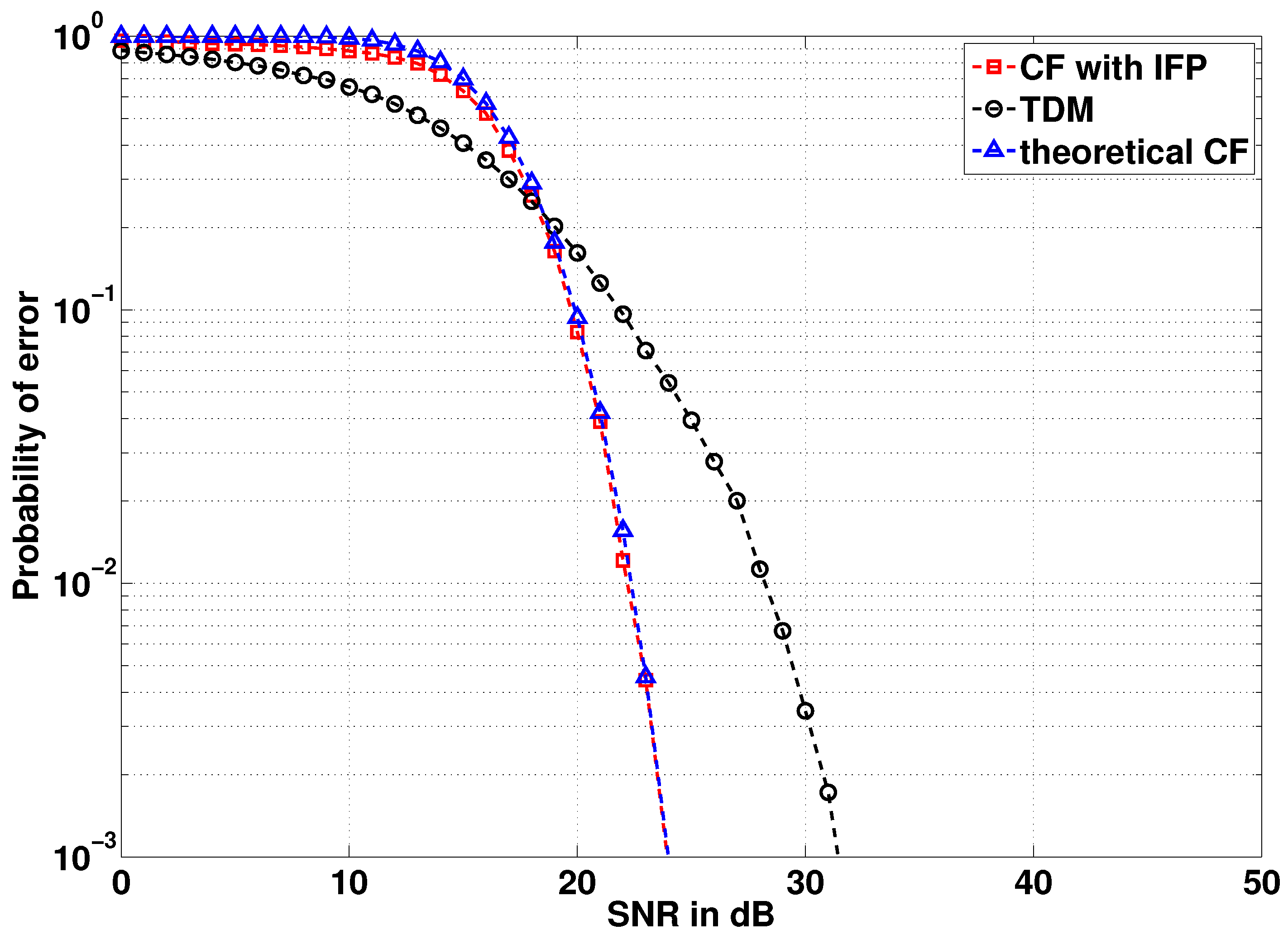
• We analyze the two phases of transmission in the CF scheme, thereby characterizing the end-to-end behavior of the CF based on different performance metrics and not only one-phase behavior, as in available studies. Compared to conventional designs, we obtain a gain of approximately 5 dB in terms of probability of error as compared to conventional time division multiplexing (TDM) transmission.

1.2. Outline of the Paper

This paper is organized as follows: Section II describes the system model and the relevant assumptions. In Section III, we present the source to relay transmission. To this end, we propose the design of an integer forcing precoder. We also present the corresponding decoding process at the relay. Section IV describes the relay-to-destination transmission modeled as a point-to-point transmission. The theoretical performance analysis of our proposed scheme is presented in Section V. The numerical results are presented in Section VI, followed by conclusions in Section VII.

1.3. Notations

We will use boldface upper case letters to denote matrices and boldface lowercase letters to indicate column vectors. Throughout the paper, $log$ indicates $log$ to the base of two. The norm, $\parallel \mathbf{x}\parallel$, denotes the $l^2$-norm of $\mathbf{x}$ given by $\parallel \mathbf{x}\parallel \stackrel{\Delta }{=}\sqrt{{\sum }_{i=1}^L\mid x\left[i\right]{\mid }^2}$. The absolute value of x is given by $\mid x\mid$. Furthermore, a diagonal matrix is denoted by $diag\left(\mathbf{x}\right)$ with the diagonal entries indicated by vector, $\mathbf{x}$.

2. System Model

We will consider an end-to-end system model for compute and forward, as shown in Figure 1. There are L sources and a single destination node, D. The L sources communicate with the destination via a single relay node, R. For the proposed precoding-based CF, transmission occurs in two phases: phase I, during which the sources transmit simultaneously to R, followed by phase II, during which R transmits to D.

Figure 1. System model.

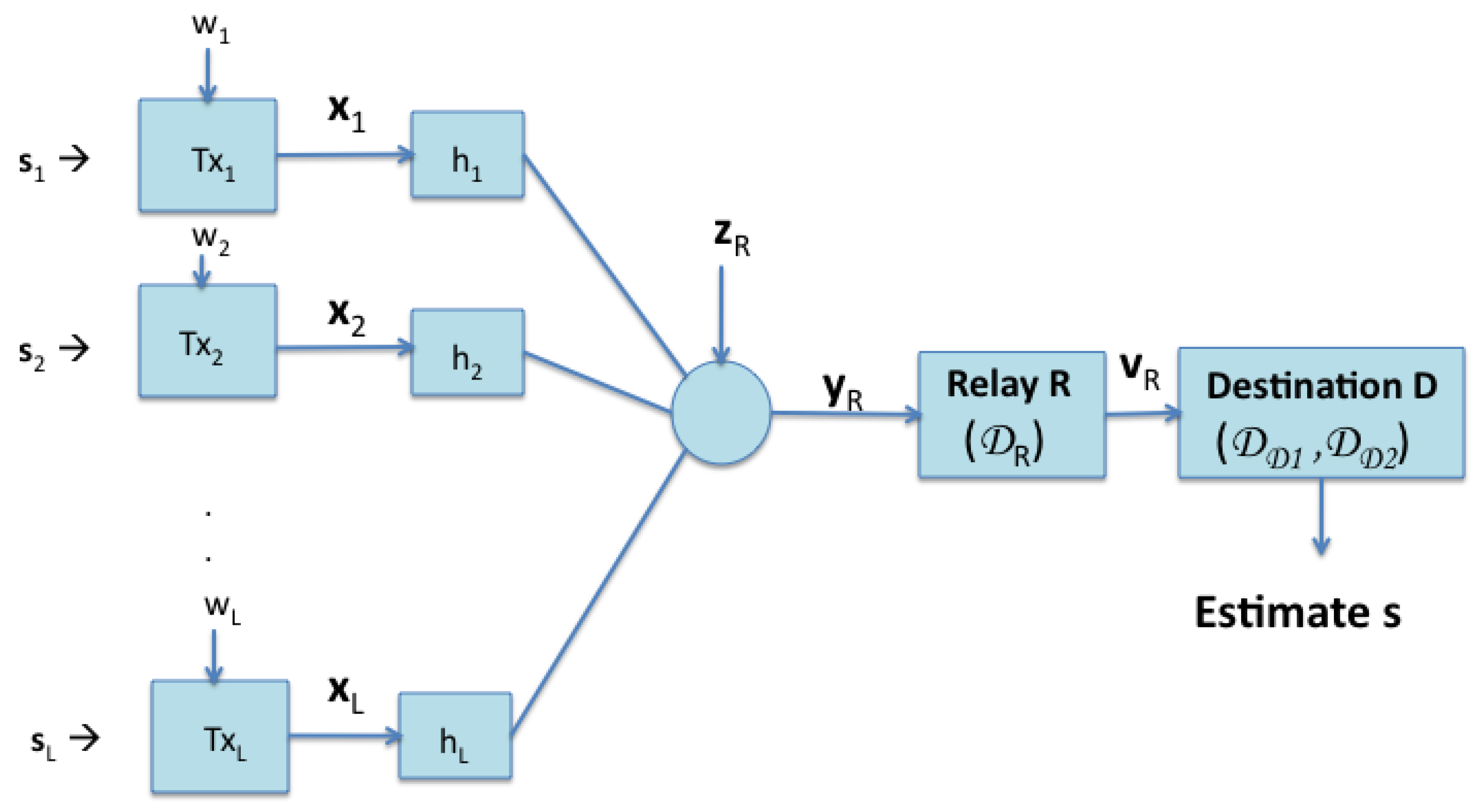
Figure 1. System model.

2.1. Phase I: Source to Relay Multiple Access Channel

Let ${\mathbf{s}}_l\in \Lambda$ be the message vector to be transmitted by $l-$th source ($l=1,\dots L$), where $\Lambda \subset \mathcal{L}$ and $\mathcal{L}=\{\lambda =\mathbf{G}\mathbf{v}\mid \mathbf{G}\in {\mathbb{R}}^{n\times n},\mathbf{v}\in {\mathbb{Z}}^n\}$ is an $n-$dimensional lattice with generator, $\mathbf{G}$, having components over time. The message vector satisfies the average power constraint:

$$\frac{1}{n}E[\parallel {\mathbf{s}}_l{\parallel }^2]=1$$

(1)

Each transmitter precodes the message signal with precoder, $w_l\in \mathbb{R}$, to obtain the precoded signal, ${\mathbf{x}}_l\in {\mathbb{R}}^n$, as:

$${\mathbf{x}}_l=w_l{\mathbf{s}}_l$$

(2)

The average power of the precoder satisfies the constraint, $E[\mid w_l{\mid }^2]\le {\gamma }_w$, where ${\gamma }_w>0$. The precoded signal satisfies the power constraint of:

$$\frac{1}{n}E[\parallel {\mathbf{x}}_l{\parallel }^2]\le {\gamma }_w$$

(3)

If ${\gamma }_w=1$, the original signal power is preserved after precoding.

The channel output, ${\mathbf{y}}_R\in {\mathbb{R}}^n$, observed at the relay is given by:

$${\mathbf{y}}_R=\sum _{l=1}^L{h}_l{\mathbf{x}}_l+{\mathbf{z}}_R$$

(4)

where $h_l\in \mathbb{R}$ is the channel coefficient between transmitter l and the relay node and ${\mathbf{z}}_R$ is i.i.d. (independent and identically distributed) Gaussian noise vector given by ${\mathbf{z}}_R={\left[\begin{array}{cccc}{z}_{R1}& z_{R2}& \dots & z_{Rn}\end{array}\right]}^T$, $z_{Ri}\sim \mathcal{N}(0,{\sigma }_1^2)$. The channel coefficient vector is given by $\mathbf{h}=\left[\begin{array}{ccc}{h}_1& \dots & h_L\end{array}\right]$, and the channel is assumed to be quasi-static. The aim of the relay is to compute a linear combination of source signals given by:

$${\mathbf{v}}_R=\sum _{l=1}^L{a}_l{\mathbf{s}}_l$$

(5)

where $a_l\in \mathbb{Z}$ are integer coefficients chosen on the basis of $h_l$. The linear coefficient vector is given by $\mathbf{a}=\left[\begin{array}{ccc}{a}_1& \dots & a_L\end{array}\right]$. The relay is free to choose these linear coefficients. Since the linear combination, ${\mathbf{v}}_R$, is computed over $\mathbb{Z}$, while the channel output is obtained over $\mathbb{R}$, the linear coefficients, $a_l$, are chosen in a way to efficiently exploit this channel output for this computation. Here, ${\mathbf{v}}_R\in {\Lambda }^{\prime }$, where:

$${\Lambda }^{\prime }=\{{\lambda }^{\prime }\mid {\lambda }^{\prime }=a_1{\lambda }_1+a_2{\lambda }_2+\dots +a_L{\lambda }_L,a_i\in \mathbb{Z},{\lambda }_i\in \Lambda \}$$

(6)

Hence, ${\Lambda }^{\prime }$ is also an $n-$dimensional lattice. The estimate of ${\mathbf{v}}_R$ obtained at the relay using the decoder, ${\mathcal{D}}_R:{\mathbb{R}}^n\to {\Lambda }^{\prime }$, is given by:

$${\widehat{\mathbf{v}}}_R={\mathcal{D}}_R\left({\mathbf{y}}_R\right)$$

(7)

It is assumed that each transmitter has the CSI of its own channel only, i.e., the channel between the transmitter itself and the relay.

2.2. Phase II: Relay-to-Destination Point-to-Point Channel

In phase II, the relay transmits the linear combination estimated in Equation (7) to the destination, D. The channel output observed at the destination, ${\mathbf{y}}_D\in {\mathbb{R}}^n$, is given by:

$${\mathbf{y}}_D=h_{RD}{\widehat{\mathbf{v}}}_R+{\mathbf{z}}_D$$

(8)

where $h_{RD}\in \mathbb{R}$ is the channel coefficient between the relay node and the destination. We assume that $h_{RD}$ is a uniformly distributed Gaussian variable with mean, ${\mu }_{h_{RD}}$, and variance, ${\sigma }_{h_{RD}}^2$, such that $h_{RD}\sim \mathcal{N}({\mu }_{h_{RD}},{\sigma }_{h_{RD}}^2)$. The additive i.i.d. Gaussian noise vector is given by ${\mathbf{z}}_D={\left[\begin{array}{cccc}{z}_{D1}& z_{D2}& \dots & z_{Dn}\end{array}\right]}^T$, $z_{Di}\sim \mathcal{N}(0,{\sigma }_2^2)$. Consequently, the estimate of ${\widehat{\mathbf{v}}}_R$ obtained at the destination using the decoder, ${\mathcal{D}}_D:{\mathbb{R}}^n\to {\Lambda }^{\prime }$, is given by:

$${\widehat{\mathbf{v}}}_D={\mathcal{D}}_{D1}\left({\mathbf{y}}_D\right)$$

(9)

The destination obtains a linear combination of the original source signals at the end of two-phase transmission. In order to decode the original source signals, the destination node collects L such linear combinations. After L repeated transmissions of their respective message from the L sources, the destination obtains L linear combinations of L source messages. Using these linear combinations, the destination decodes the original source messages using the decoder:

$$\widehat{\mathbf{s}}={\mathcal{D}}_{D2}\left(\mathbf{v}\right)$$

(10)

where $\mathbf{v}=\left[\begin{array}{ccc}{\widehat{\mathbf{v}}}_D^1& \dots & {\widehat{\mathbf{v}}}_D^L\end{array}\right]$ is the matrix containing L linear combinations obtained at the destination. ${\widehat{\mathbf{v}}}_D^l$ denotes the lth linear combination obtained at the destination. The original message matrix estimated at the destination is given by $\widehat{\mathbf{s}}=\left[\begin{array}{ccc}{\widehat{\mathbf{s}}}_1& \dots & {\widehat{\mathbf{s}}}_L\end{array}\right]$. Note that in this paper, we focus on a real-valued system model for simplicity; however, we assert that the work can be extended to a complex-valued system.

3. Phase I : Proposed Precoding-Based Source to Relay Transmission

In this section, we focus upon transmission phase I from the L sources to the relay node. Each of the L sources transmits a lattice point from the same lattice towards the relay nodes. The received signal at the relay is a noisy linear combination of the lattice points, with linear coefficients given by the channel gains. As explained in Section 1, the concept of CF relies on the lattice property that an integral linear combination of lattice points is another lattice point. However, the received signal at the relay does not necessarily have integral coefficients, as the natural channel gains are not necessarily integers. Therefore, the closest lattice point to the received signal may or may not be an integral linear combination of the original lattice points, depending on the additive noise and the “self-noise” contributed by the non-integral nature of the channel. Since additive noise is inherent to the system, the self-noise due to the non-integral nature of the channel should be minimized. In this section, the problem of obtaining an integer linear combination of original signals from the received signal is formulated, and subsequently, an integer forcing precoder design is proposed.

3.1. Problem Formulation

The aim of a precoding-based implementation of CF is to obtain the linear combination of original signals at the relay without incurring the errors due to approximation of the channel by integers. To this end, the precoder is used to shift the channel coefficients to the closest possible integer using the CSI at the transmitter. Therefore, consider a channel decomposition as:

$$h_l=h_l^z+h_l^{\overline{z}}$$

(11)

where $h_l^z\in \mathbb{Z}$ is an integer approximation of $h_l$ and, consequently, $h_l^{\overline{z}}\in \mathbb{R}$. Using Equations (2) and (11), we can rewrite Equation (4) as:

$${\mathbf{y}}_R=\sum _{l=1}^L{h}_l{w}_l{\mathbf{s}}_l+{\mathbf{z}}_R+\sum _{l=1}^L{h}_l^z{\mathbf{s}}_l-\sum _{l=1}^L{h}_l^z{\mathbf{s}}_l$$

which can be simplified as:

$${\mathbf{y}}_R=\underset{{\mathbf{v}}_{eff}}{\underbrace{\sum _{l=1}^L{h}_l^z{\mathbf{s}}_l}}+\underset{{\mathbf{z}}_{eff}}{\underbrace{\sum _{l=1}^L(h_l{w}_l-h_l^z){\mathbf{s}}_l+{\mathbf{z}}_R}}$$

(12)

The relay aims to decode ${\mathbf{v}}_{eff}$ from ${\mathbf{y}}_R$. The effective noise, ${\mathbf{z}}_{eff}$, is comprised of the receiver noise (${\mathbf{z}}_R$) and the additional “self-noise”, arising due to the difference between the real channel and its integral approximation. Using the rate of computation derived in [2], we can write the rate of computation of the linear combination of original signals as:

$$R(\mathbf{h},\mathbf{w})={log}^{+}\left(\frac{P}{1+P{\sum }_{l=1}^L{(h_l{w}_l-h_l^z)}^2}\right)$$

where ${\log }^{+}\left(x\right)=max(0,\log \left(x\right))$, P is the signal to noise ratio given by $P=1/{\sigma }_1^2$ and $\mathbf{w}=\left[\begin{array}{cccc}{w}_1& w_2& \dots & w_L\end{array}\right]$. Therefore:

$$R(\mathbf{h},\mathbf{w})={log}^{+}\left(\frac{1}{{\sigma }_1^2+{\sum }_{l=1}^L{(h_l{w}_l-h_l^z)}^2}\right)$$

Using the power constraints, the rate can be rewritten as:

$$R(\mathbf{h},\mathbf{w})={\log }^{+}\left(\frac{1}{{\sigma }_1^2+\parallel \mathbf{hW}-{\mathbf{h}}^z{\parallel }^2}\right)$$

where ${\mathbf{h}}^z=\left[\begin{array}{ccc}{h}_1^z& \dots & h_L^z\end{array}\right]$ and $\mathbf{W}=diag\left(\mathbf{w}\right)$. It is assumed that $h_l^z\ne 0$, to ensure that the linear combination has non-zero coefficient of each of the L messages; therefore, $\parallel {\mathbf{h}}^z\parallel \ge 1$. Hence, we obtain:

$$R(\mathbf{h},\mathbf{w})\le {\log }^{+}\left(\frac{\parallel {\mathbf{h}}^z{\parallel }^2}{{\sigma }_1^2+\parallel \mathbf{hW}-{\mathbf{h}}^z{\parallel }^2}\right)$$

(13)

Hence, the precoder, $w_l$, should be designed such that it is able to minimize ${\mathbf{z}}_{eff}$ in Equation (12) and maximize the achievable rate in Equation (13). The design of such a precoder is proposed in the next subsection.

3.2. Proposed Integer Forcing Precoder

We aim to precode the signals, such that a linear combination of original signals can be obtained at the relay at the maximum rate. It is well known that zero forcing (ZF) precoding is a standard suboptimal approach for precoding, which is known to provide a promising trade-off between complexity and performance [11]. The traditional zero forcing precoder is designed to eliminate the effect of the channel fading, while satisfying constraints of power optimally as per certain performance measures.

The precoder required in implementing CF has similar design requirements as ZF precoding, but with an important difference. In CF, the precoder is required to eliminate only the non-integral part of the channel, while retaining the integral part in the precoded signal. In this subsection, we show the design of a naive precoder to implement CF.

A sub-optimal integer forcing precoder (IFP) that maximizes the rate of computation, while eliminating the non-integral part of the channel, is given by the solution to the following optimization problem:

$$\underset{{\mathbf{h}}^{\mathbf{z}}\in {\mathbb{Z}}^L,{\mathbf{h}}^{\mathbf{z}}\ne 0}{max}R(\mathbf{h},\mathbf{w})$$

(14)

$$\mathrm{subject}\mathrm{to}E[\mid w_l{\mid }^2]\le {\gamma }_w$$

(15)

In order to solve this problem, we relaxed condition (15), making it an unconstrained optimization problem. A direct differentiation of $R(\mathbf{h},\mathbf{w})$ with respect to $\mathbf{W}$ gives:

$${\mathbf{W}}_{opt}=diag\left({\mathbf{h}}^{-1}{\mathbf{h}}_{opt}^{\mathbf{z}}\right)$$

where ${\mathbf{h}}_{opt}^{\mathbf{z}}$ is the solution to:

$$\underset{{\mathbf{h}}^{\mathbf{z}}\in {\mathbb{Z}}^L,{\mathbf{h}}^{\mathbf{z}}\ne 0}{max}{\log }^{+}\left(\frac{\parallel {\mathbf{h}}^z{\parallel }^2}{{\sigma }_1^2}\right)$$

(16)

$$\mathrm{subject}\mathrm{to}E[\mid h_l^z{h}_l^{-1}\mid ]{}^2<{\gamma }_w\mathrm{for}l=1\dots L$$

(17)

Hence, the integer part of the channel, ${\mathbf{h}}^{\mathbf{z}}$, should be chosen, such that, within the constraint of maximum precoding power, ${\gamma }_w$ , the computational rate is maximized. A possible solution is given by (rounding off using the Babai estimate [12]):

$${\mathbf{h}}_{opt}^{\mathbf{z}}=\left[{\gamma }_w\mathbf{h}\right]$$

(18)

where $\left[.\right]$ represents the closest integer. Without loss of generality, one of the solutions can be taken as ${\mathbf{h}}_{opt}^{\mathbf{z}}=\left[\mathbf{h}\right]$. The resultant precoder, which also imposes the constraint, ${\mathbf{h}}^{\mathbf{z}}\ne 0$, is given by:

$$w_l=\left\{\begin{array}{cc}\begin{array}{cc}\frac{h_l^z}{h_l},& \mid h_l\mid >0.5\\ \\ \frac{1}{h_l},& \mid h_l\mid \le 0.5\end{array}\hfill & \mathrm{for}l=1\dots L\hfill \end{array}\right.$$

(19)

This solution maximizes the rate Equation (13), because $h_l^z$ is the closest integer to the channel, $h_l$. Note that, here, each transmitter precodes the signal by imposing $h_l^z\ne 0$, thereby making the probability of the condition, ${\mathbf{h}}^{\mathbf{z}}=0$, to become strictly zero. Since we have assumed that the lth transmitter is aware of only the $h_l$ channel coefficient, therefore, simply imposing $h_l^z\ne 0$ ensures that ${\mathbf{h}}^{\mathbf{z}}\ne 0$.

In the next theorem, it is shown that the proposed IFP eliminates the additional self-noise in CF.

Theorem 1: The IFP can completely eliminate the additional self-noise in the CF scheme with an upper bounded power penalty for the channel with reasonable gains.

Proof: Firstly, to prove the elimination of self-noise by the use of IFP, the received signal in Equation (4) is rewritten, using Equation (19), as:

$${\mathbf{y}}_R=\sum _{l=1}^L{h}_l{w}_l{\mathbf{s}}_l+{\mathbf{z}}_R=\sum _{l=1}^L{h}_l^z{\mathbf{s}}_l+{\mathbf{z}}_R$$

Assuming ${\mathbf{v}}_R={\sum }_{l=1}^L{h}_l^z{\mathbf{s}}_l$, the received signal is given by:

$${\mathbf{y}}_R={\mathbf{v}}_R+{\mathbf{z}}_R$$

(20)

The effective noise is clearly only Gaussian noise, and the self-noise is completely eliminated. However, the use of IFP requires an extra power penalty at the transmitter.

Next, to prove that this additional required power is within finite range for any channel, the proposed precoder in Equation (19) can be written as:

$$w_l=\frac{1}{1+r}$$

where $r=h_l^{\overline{z}}/h_l^z$. Since $h_l^z\in \mathbb{Z}$ and $h_l^{\overline{z}}\in (-0.5,0.5)$ for $\mid h_l\mid >0.5$, therefore, the range of r is given by $r\in (-0.5,0.5)$. Putting r in the expression of $w_l$ above, we get the range of $w_l$ as $w_l\in (\frac{2}{3},2)$. Consequently, the range of $w_l^2$ is given by $w_l^2\in \left(\frac{4}{9},4\right)$. In the limiting condition, the upper bound of the average precoder power, $E[\mid w_l{\mid }^2]={\gamma }_w$ (using the power limitation from (3)), can be given as:

$$\frac{4}{9}<{\gamma }_w<4$$

(21)

Hence, the precoded signal power using the proposed IFP is bounded for channel realization with reasonably good gains. This concludes our proof.

Remark: From theorem 1, it can be seen that the use of IFP to implement CF effectively reduces the channel to a reliable AWGN (additive white Gaussian noise) channel. Therefore, the achievable rate using the above IFP is given by:

$$R_{IFP}\left(\mathbf{h}\right)\le {\log }^{+}\left(\frac{\parallel {\mathbf{h}}^z{\parallel }^2}{{\sigma }_1^2}\right)$$

(22)

From Equations (2) and (21), it is clear that when ${\gamma }_w=1$, the power consumed by the precoded signal is equal to the power consumed by the original signal under limiting conditions. However, when ${\gamma }_w<1$ (or equivalently, $h_l^z<h_l$), the precoded signal consumes less power than the original signal. On the other hand, when ${\gamma }_w>1$, the precoded signal consumes additional power. If this additional power is not available at the transmitter, the precoding may fail. We study this case in detail under outage formulation in Section VI.

With a finite power penalty, the proposed IFP can convert the signal obtained at the relay into a reliable linear combination of source messages. The decoder at the relay employs the maximum likelihood (ML) decoding to obtain a linear combination of source messages, as explained in the next subsection.

3.3. Decoding at the Relay

We aim to apply ML decoding on the received signal at the relay. According to Theorem 1, the received signal is given by ${\mathbf{y}}_R={\mathbf{v}}_R+{\mathbf{z}}_R$, where ${\mathbf{v}}_R={\sum }_{l=1}^L{h}_l^z{\mathbf{s}}_l$ and ${\mathbf{z}}_R\sim \mathcal{N}(0,{\sigma }_1^2{\mathbf{I}}_n)$. The linear combination of signals, ${\mathbf{v}}_R\in {\Lambda }^{\prime }$, such that:

$${\Lambda }^{\prime }=\{{\lambda }^{\prime }\mid {\lambda }^{\prime }=h_1^z{\lambda }_1+h_2^z{\lambda }_2+\dots +h_L^z{\lambda }_L,h_i^z\in \mathbb{Z},{\lambda }_i\in \Lambda \}$$

(23)

By the properties of lattices [13], a linear combination of lattice points gives another lattice point; therefore, ${\Lambda }^{\prime }\subseteq \mathcal{L}$. The ML decoder, ${\mathcal{D}}_R(.)$, in Equation (7) gives the estimate of ${\mathbf{v}}_R$ as:

$${\widehat{\mathbf{v}}}_R={\mathcal{D}}_R\left({\mathbf{y}}_R\right)=arg\underset{\mathbf{t}\in {\Lambda }^{\prime }}{min}\parallel {\mathbf{y}}_R-\mathbf{t}{\parallel }^2$$

A low complexity sphere decoder [12] can be used to perform ML decoding. Note that the decoder architecture reflects a point-to-point AWGN channel with input, ${\mathbf{v}}_R$, and additive channel noise. This shows that the complexity of the decoder architecture is equivalent to the decoder complexity of the point-to-point channel.

4. Phase II: Proposed Point-to-Point Relay-to-Destination Transmission

In this section, we describe phase II of the transmission of the proposed precoding-based CF scheme between the relay node and the destination node.

4.1. Problem Formulation

The computation of original signals at the destination is a two-fold problem: firstly, the destination node decodes the linear combination obtained from the relay node, and secondly, after obtaining sufficient linear combinations, the destination node decodes the original source signals. Therefore, we formulate the two problems at the decoder and propose the respective solutions using two decoders, namely ${\mathcal{D}}_{D1}$ and ${\mathcal{D}}_{D2}$, respectively, in subsequent subsections.

The first aim of the destination is to obtain the linear combination estimated at the relay from the noisy signal obtained from the channel. We recall that the received signal at the destination is given by Equation (8):

$${\mathbf{y}}_D=h_{RD}{\widehat{\mathbf{v}}}_R+{\mathbf{z}}_D$$

The destination node aims to obtain the linear combination, ${\widehat{\mathbf{v}}}_R$. To this end, the received signal is equalized using an equalizer, α, and a suitable decoder is used to obtain the linear combination. Therefore, the first decoder in Equation (9) is given as:

$${\widehat{\mathbf{v}}}_D={\mathcal{D}}_{D1}(\alpha ,{\mathbf{y}}_D)$$

Therefore, the primary problem at the destination is to obtain a decoder suitable for the above decoding.

The next aim of the destination is to obtain the original source signals from the L linear combinations obtained. Therefore, the matrix of the linear combinations after L transmissions given by $\mathbf{v}={\left[\begin{array}{ccc}{\widehat{\mathbf{v}}}_D^1& \dots & {\widehat{\mathbf{v}}}_D^L\end{array}\right]}^T$ is supplied to the second decoder at the destination, which obtains the estimate of the original source signal matrix, given by $\mathbf{s}={\left[\begin{array}{ccc}{\mathbf{s}}_1& \dots & {\mathbf{s}}_L\end{array}\right]}^T$, such that:

$$\widehat{\mathbf{s}}={\mathcal{D}}_{D2}\left(\mathbf{v}\right)$$

The second problem at the destination is to obtain the design of a decoder to obtain the original source signals.

4.2. Decoding Linear Combination at the Destination

In order to obtain the decoder at the destination to obtain the linear combination of the original signals from the noisy channel output, we propose to use a zero forcing equalizer. Therefore, for this decoding, we set α, such that $\alpha =\frac{1}{h_{RD}}$, which leads to the equalized signal being:

$$\alpha {\mathbf{y}}_D={\widehat{\mathbf{v}}}_R+\frac{{\mathbf{z}}_D}{h_{RD}}$$

(24)

Consequently, an ML decoder is used to obtain ${\widehat{\mathbf{v}}}_R$. A low complexity ML decoder, namely a sphere decoder, can be used to perform the decoding operation. The ML decoder, designed identically to the sphere decoder used at the relay as the lattice to which the target decoded signal, ${\mathbf{v}}_R$, belongs, is the same at both the relay and the destination node. Therefore:

$${\widehat{\mathbf{v}}}_D={\mathcal{D}}_{D1}(\alpha ,{\mathbf{y}}_D)={\arg \min }_{\mathbf{t}\in {\Lambda }^{\prime }}\parallel \alpha {\mathbf{y}}_D-\mathbf{t}{\parallel }^2$$

where ${\Lambda }^{\prime }$ is given by Equation (23). Note that the decoding is without error, as long as $\frac{z_D}{h_{RD}}$ in Equation (24) is within the Voronoi region of the lattice, ${\Lambda }^{\prime }$. We explore the probability of error in the detection of linear combination in Section V.

4.3. Decoding Original Signals at the Destination

In order to detect the original source signals, the destination node requires collecting L independent linear combinations. After L transmissions, the destination obtains L linear combinations of L messages from L users. Using these linear combinations, the destination decodes the original source messages using the decoder given in Equation (10). In order to design the decoder, we rewrite the L linear combinations as (for each dimension):

$$\underset{\mathbf{v}}{\underbrace{\left[\begin{array}{c}{\widehat{v}}_D^1\\ ⋮\\ {\widehat{v}}_D^L\end{array}\right]}}=\underset{\mathbf{A}}{\underbrace{\left[\begin{array}{ccc}{a}_1^1& \dots & a_L^1\\ ⋮& \dots & ⋮\\ a_1^L& \dots & a_L^L\end{array}\right]}}\underset{\mathbf{s}}{\underbrace{\left[\begin{array}{c}{s}_1\\ ⋮\\ s_L\end{array}\right]}}$$

Here, ${\widehat{v}}_D^l$ denotes the l-th linear combination element estimated at the destination. Furthermore, $a_k^l$ denotes the linear coefficient of the kth source signal in the lth linear combination. The matrix, $\mathbf{A}$, contains the integer linear coefficients of the linear combinations. If $\mathbf{A}$ is full rank, $\mathbf{s}$ is obtained by inverting $\mathbf{A}$, such that:

$$\widehat{\mathbf{s}}={\mathcal{D}}_{D2}\left(\mathbf{v}\right)={\mathbf{A}}^{-1}\mathbf{v}$$

where $\widehat{\mathbf{s}}$ is the estimate of the original source signals. It is assumed that, since the channel conditions are highly variant (typically in vehicular networks), the channel fades independently in each transmission. Consequently, the matrix formed by the rounded channel coefficients is full rank with high probability. As proposed in our scheme, the transmitter chooses the integer coefficients closest to the channel coefficients; therefore, $\mathbf{A}$ is full rank with high probability.

5. Performance Analysis

In this section, we analyze the proposed precoding-based CF implementation under light of the probability of error. Note that we will make use of the geometrical properties of lattices in obtaining closed form expressions of the probability of error [14,15].

The end-to-end probability of error of the precoded CF is culminated by two error probabilities: (i) the probability of error from the source to relay node and (ii) the probability of error from the relay to destination node. In this subsection, we obtain two probabilities separately and, then, formulate the end-to-end probability of the error expression.

5.1. Probability of Error from Source to Relay Node

According to Theorem 1, the received signal at the relay is the linear combination of original signals with additive Gaussian noise. Therefore, an error occurs if the noise vector is outside the fundamental Voronoi region [14] of the lattice, ${\Lambda }^{\prime }$, in Equation (23), denoted by $\mathcal{V}\left({\Lambda }^{\prime }\right)$. The probability of error in decoding a linear equation in $n-$dimensional lattice at the relay is given by:

$$P_1(\mathbf{h},n)=\mathrm{Pr}(\parallel {\mathbf{z}}_R\parallel \notin \mathcal{V}\left({\Lambda }^{\prime }\right))$$

(25)

The vector, ${\mathbf{z}}_R$, has Gaussian distribution in each dimension with zero mean and variance, ${\sigma }_1^2$. It is well known that the above probability expression depends on the shape of the Voronoi region. The bounds of such probability of error can be found in [16].

For simplicity, we now consider a subset of an integer lattice, namely, $\mathcal{L}={\mathbb{Z}}^n$, to draw the original signals, $s_l$. This is because the Voronoi region for the integer lattice is a hypercube, and hence, it can be used to obtain an exact probability of the error expression. The following theorem gives this probability.

Theorem 2: The probability of error in decoding a linear equation of signals drawn from $\mathcal{L}={\mathbb{Z}}^n$ using IFP is given by:

$$P_1(\mathbf{h},n)=1-{\left(\mathrm{erf}\left(\frac{c}{2\sqrt{2}{\sigma }_1}\right)\right)}^n$$

where $c=\gcd (h_1^z,h_2^z,\dots ,h_L^z)$

Proof: We firstly use induction to prove the that the Voronoi region of ${\Lambda }^{\prime }=\{{\lambda }^{\prime }\mid {\lambda }^{\prime }={\sum }_{l=1}^L{h}_l^z{\lambda }_l,h_i^z\in \mathbb{Z},{\lambda }_i\in \Lambda \}$ is a hypercube of side c. Let $L=2$ and $n=1$. The Bezout’s lemma [17] states that for any two (non-zero) integers, p and q, there exist two integers, u and v, such that

$$pu+qv=d,$$

where d is the common divisor of p and q. In addition, if $d>0$ is the greatest common divisor (gcd) of ($p,q$), it is the smallest positive integer satisfying this equation for any $(u,v)$ integer pair. Therefore, using Bezout’s lemma, any point in ${\Lambda }^{\prime }$ can be written as:

$${\lambda }^{\prime }=b_1{\lambda }_1+b_2{\lambda }_2=d\mathbb{Z}$$

where $d=\gcd (b_1,b_2)$. Similarly, this result can be extended to $L=L+1$ by induction. Since this result is independent of the integers, ${\lambda }_i$, therefore, it can be extended to $n-$dimensional lattices. Using this result, we can write:

$${\Lambda }^{\prime }=c{\mathbb{Z}}^n$$

where $c=\gcd (h_1^z,h_2^z,\dots ,h_L^z)$. Hence, the Voronoi region of ${\Lambda }^{\prime }$ is a hypercube of side c.

To prove the second part of the theorem, we rewrite Equation (25) as:

$$P_1(\mathbf{h},n)=1-\mathrm{Pr}(\parallel \mathbf{z}\parallel \in \mathcal{V}\left({\Lambda }^{\prime }\right))$$

$$=1-{\left(\frac{1}{\sqrt{2\pi {\sigma }^2}}\underset{-c/2}{\overset{c/2}{\int }}{e}^{-\frac{u^2}{2{\sigma }_1^2}}du\right)}^n$$

$$P_1(\mathbf{h},n)=1-{\left(\mathrm{erf}\left(\frac{c}{2\sqrt{2}{\sigma }_1}\right)\right)}^n$$

(26)

where $\mathrm{erf}\left(x\right)=\frac{2}{\sqrt{\pi }}{\int }_0^x{e}^{-t^2}dt$. This concludes our proof.

For the special case of $n=1$, Equation (26) reduces to:

$$P_1(\mathbf{h},1)=\mathrm{erfc}\left(\frac{c}{2\sqrt{2}{\sigma }_1}\right)$$

(27)

where $\mathrm{erfc}\left(x\right)=1-\mathrm{erf}\left(x\right)$.

Note that in the proposed scheme, the effective behavior of the channel is reduced to a point-to-point AWGN channel with no channel fading. This makes its characterization possible. In the previous formulations of CF, the effective noise is Gaussian noise along with the self-noise, which results in the non-Gaussian distribution of total effective noise [5]. Hence, the characterization in existent formulations has been done by providing limits of error probability and not the accurate value. However, with IFP, CF can be implemented without the limitation of any self-noise adding to the effective noise. However, the penalty that is paid is the extra power required at the transmitter. We analyze the effect of this penalty on performance in terms of outage probability in the next section.

5.2. Probability of Error from Relay-to-Destination Node

The signal received at the destination, given by Equation (8), is normalized to the channel coefficient, resulting in:

$$\frac{{\mathbf{y}}_D}{h_{RD}}={\widehat{\mathbf{v}}}_R+\frac{{\mathbf{z}}_D}{h_{RD}}$$

(28)

The following theorem gives the probability of error at the destination node.

Theorem 3: The probability of error in decoding the linear combination of signals sent from the relay to the destination for $\mathcal{L}={\mathbb{Z}}^n$ is given by:

$$P_2(d,n)=1-{\left(\frac{2}{\pi }\left(arctan\left(\frac{1}{2d}\right)\right)\right)}^n$$

where $d=\frac{{\sigma }_2}{{\sigma }_{h_{RD}}}$, such that $h_{RD}\sim \mathcal{N}(0,{\sigma }_{h_{RD}}^2)$, and the variance of added noise is ${\sigma }_2^2$.

Proof: Using Equation (28), the probability of error at the destination is given by:

$$P_2(d,n)=Pr\left(∥\frac{{\mathbf{z}}_D}{h_{RD}}∥\notin \mathcal{V}\left({\Lambda }^{\prime }\right)\right)$$

where ${\Lambda }^{\prime }$ is defined in Equation (23). The distribution of ${\mathbf{z}}_D/h_{RD}$ is the quotient of two normal distributions with zero mean. Such a distribution is given by the Cauchy’s distribution [18] with zero mean. Let us define ratio d as $d=\frac{{\sigma }_2}{{\sigma }_{h_{RD}}}$. The probability density function of Cauchy’s distribution takes the form of:

$$\varphi \left(x\right)=\frac{d}{\pi (x^2+d^2)}$$

An error occurs in the decoding if the noise falls outside the Voronoi region. Therefore, we integrate the distribution of effective noise from (−1/2,1/2) to obtain the probability of error-free transmission and, consequently, subtract it from one to find the probability of error. Hence, the resulting expression is given by:

$$P_2(d,n)=1-{\left({\int }_{-1/2}^{1/2}\varphi \left(x\right)dx\right)}^n$$

The above integration can be written as:

$$P_2(d,n)=1-{\left({\int }_{-1/2}^{1/2}\frac{d}{\pi (x^2+d^2)}dx\right)}^n$$

Using $\frac{1}{x^2+a^2}dx=\frac{1}{a}arctan\frac{x}{a}+C$, we get:

$$P_2(d,n)=1-{\left(\frac{d}{\pi }\left(\frac{1}{d}arctan\left(\frac{1}{2d}\right)-\frac{1}{d}arctan\left(-\frac{1}{2d}\right)\right)\right)}^n$$

Since $arctan(-x)=-arctan\left(x\right)$, therefore:

$$P_2(d,n)=1-{\left(\frac{2}{\pi }\left(arctan\left(\frac{1}{2d}\right)\right)\right)}^n$$

(29)

where $d=\frac{{\sigma }_2}{{\sigma }_{h_{RD}}}$.

For the special case of $n=1$, the above reduces to:

$$P_2(d,1)=1-\frac{2}{\pi }\left(arctan\left(\frac{1}{2d}\right)\right)$$

We now give the overall probability of error.

5.3. Overall End-to-End Probability of Error

We now aim to evaluate the overall probability of error for CF. An error occurs in CF transmission if the linear combination of source signals is not correctly obtained at the relay and/or the linear combination transmitted from the relay is not correctly obtained at the destination. Hence, both the phases of transmissions are required to be free from error. Further, the entire scheme requires L transmissions, because L linear combinations are required at the destination to obtain the original signals. Hence, the CF transmission is successful if and only if L-independent linear combinations are obtained at the destination without any error. Since we assumed that the channel is highly variant in time, hence, it is implicit that the L linear combinations will be independent. Therefore, the overall probability of error for CF scheme is given by (for $n=$1 dimension):

$$P_e=1-\prod _{l=1}^L(1-P_1^l)(1-P_2^l)$$

where the superscript indicates the $l-$th transmission. Therefore, inserting the expressions for $P_1$ and $P_2$ from Equations (26) and (29), respectively, we obtain:

$$P_e=1-{\left(\frac{2}{\pi }\left(arctan\left(\frac{1}{2d}\right)\right)\right)}^L\prod _{l=1}^L\left(1-\mathrm{erfc}\left(\frac{c^l}{2\sqrt{2}{\sigma }_1}\right)\right)$$

(30)

As in previous cases, the superscript indicates the value of the variable in the lth transmission. The above expression takes into account the necessity of all the linear combinations to be simultaneously error-free for error-free transmission. A simplified upper bound to the above expression can be given by (assuming a fixed gcd of one for all channel realizations):

$$P_e^u=1-{\left(\frac{2}{\pi }\left(arctan\left(\frac{1}{2d}\right)\right)\right)}^L{\left(1-erfc\left(\frac{1}{2\sqrt{2}{\sigma }_1}\right)\right)}^L$$

(31)

In the next section, we will present the numerical results to demonstrate the performance of the proposed scheme.

6. Numerical Results

In this section, we demonstrate the performance of the proposed scheme with the help of numerical simulations. We focus on mainly three performance metrics: (i) probability of error; (ii) achievable rates; and (iii) outage probability.

6.1. Probability of Error

In order to analyze the probability of error performance for the proposed IFP, we perform the simulations under two parts. In the first part, we study the stand-alone performance of the IFP precoder by observing the probability of error behavior at the relay node. Further, in the second part, we analyze the effect of the implementation of CF with IFP on the overall end-to-end system from source to destination.

6.1.1. Probability of Error at the Relay

Two sources are considered to be transmitting the signals ($s_1$ and $s_2$) drawn from a one-dimensional integer lattice, i.e., $n=1$ and $\mathcal{L}=\mathbb{Z}$. There is one relay, which decodes the linear combination of these signals. The performance in terms of probability of error in decoding the linear combination of original signals at the relay is simulated. The additive noise at the relay node has a Gaussian distribution.

In order to compare with the existent schemes, the baseline lattice network coding (LNC) scheme, which is used to practically implement CF in [3], is considered. To make a fair comparison, we have adjusted the power of the transmitters in the schemes with and without precoding, such that the total power available at the transmitters in both schemes is equal. We consider precisely the same channel as considered in [5], for the sake of comparison, given by $\mathbf{h}=\left[\begin{array}{cc}-1.274& 0.602\end{array}\right]$; however, the results are not sensitive to the choice of the channel gain vector.

We observe in Figure 2 that the probability of error by the proposed IFP-based scheme has a gain of up to 2 dB over the existent baseline LNC.

For comparison, we also plot the probability of error, which can be achieved when the channel gain vector is integral. In this case, the additional noise is the only source of error at the relay. Therefore, this indicates a lower bound of the probability of error for CF. Note that, with our proposed precoding, the only source of error at the relay is the additional noise. However, as shown in Figure 2, there is a gap between the proposed scheme and the lower bound. This gap is due to the penalty of extra power required for precoding. More precisely, the proposed scheme requires more power at the transmitter to achieve the same probability of error as the CF with an integral channel.

Figure 2. Comparison of the probability of error at the relay for the proposed scheme with varying signal to noise ratio (SNR) for $L=2$. The total signal power is adjusted for fair comparison with other schemes.

Figure 2. Comparison of the probability of error at the relay for the proposed scheme with varying signal to noise ratio (SNR) for $L=2$. The total signal power is adjusted for fair comparison with other schemes.

6.1.2. Probability of Error at the Destination

In order to analyze the overall performance of using IFP with the CF system, we consider the extension of the above model to the destination node. The aim of the destination is to obtain L original source signals. Hence, we consider L transmissions to study the performance of error at the destination. After L transmissions from source to relay, the L transmissions from relay to destination are orthogonalized in time. The channel from relay to destination is a random real valued channel. Figure 3 shows the probability of error of CF implemented with IFP. To make a comparison with the state-of-the-art , we plot the error performance of the system when Time Division Multiplexing (TDM) is used to transmit the signals from source to destination via relay. In the case of TDM, one source transmits at one time instant to the relay. The relay decodes the signals and sends it to the destination. In the next time instant, the relay sends the decoded signal to the destination, and the destination decodes the original signal from the first source. After $L+1$ time slots, all the L signals are received at the destination. Figure 3 shows that CF with IFP shows a gain of approximately 5 dB at an error of 1% over TDM. This gain is basically due to multiple copies of the same signals received at the relay in the case of CF with IFP, which is not the case in TDM. Hence, in case the channel is in a deep fade, it results in an error in TDM, whereas such deep fading situations are overcome, due to the existence of multiple copies of the same signals in CF. Note that we have again considered fixed channel gains here, which reduces the theoretical integration of equalized noise in Equation (28) to a point-to-point error probability expression.

Figure 3. Compute and forward (CF) with the integer forcing precoder (IFP) compared to Time Division Multiplexing (TDM) performance at the destination.

Figure 3. Compute and forward (CF) with the integer forcing precoder (IFP) compared to Time Division Multiplexing (TDM) performance at the destination.

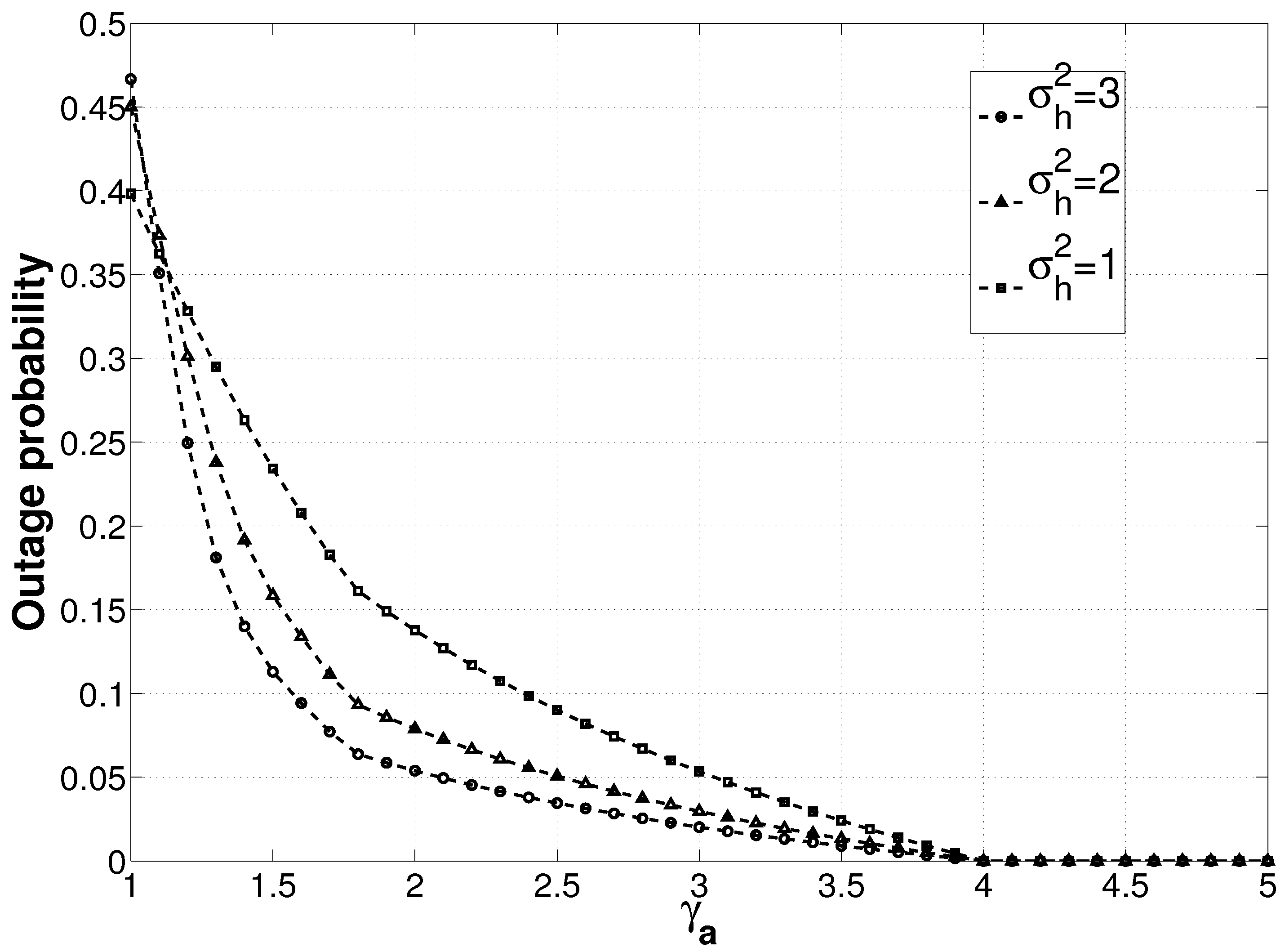
6.2. Outage Probability

In this subsection, we formulate the probability of an outage event to occur in the system. When the total power available at the transmitter is limited, the integer forcing precoding may fail, depending on the total power requirement of the precoder. We define the outage probability, $P_{out}$, as the probability when the integer forcing precoding requires more power than the power available at the transmitter. Let the total power available at the transmitter be given by ${\gamma }_a$. This power, ${\gamma }_a$, is the maximum power that the transmitter can use to precode. The power required by the precoded signal is given by ${\gamma }_w$. Therefore, if the precoder is such that it needs more power to precode than the available power, ${\gamma }_a$, we have a case of outage, as:

$$P_{out}=Pr({\gamma }_w>{\gamma }_a)$$

The distribution of the above probability depends on the distribution of the channel fading coefficients, because IFP is designed as $w_l=h_l^z/h_l$. The outage probability for a Gaussian channel with varying available power has been shown in Figure 4. The outage probability decreases with increasing available power. When ${\gamma }_a>4$, the outage probability goes to zero, because ${\gamma }_w<4$, as shown in Theorem 1.

Figure 4 indicates that as the channel variance increases, the outage probability decreases. This is due to the fact that with increasing channel gain, $h_l$, the power required by the precoder decreases. Hence, the higher the instantaneous channel gain, the better is the outage performance of IFP.

Figure 4. Outage probability curve. The horizontal axis shows the power available at the transmitter. The power available at the transmitter is assumed to be always greater than or equal to the signal power, hence ${\gamma }_a>1$. With the increasing channel variance, ${\sigma }_h$, the outage decreases.

Figure 4. Outage probability curve. The horizontal axis shows the power available at the transmitter. The power available at the transmitter is assumed to be always greater than or equal to the signal power, hence ${\gamma }_a>1$. With the increasing channel variance, ${\sigma }_h$, the outage decreases.

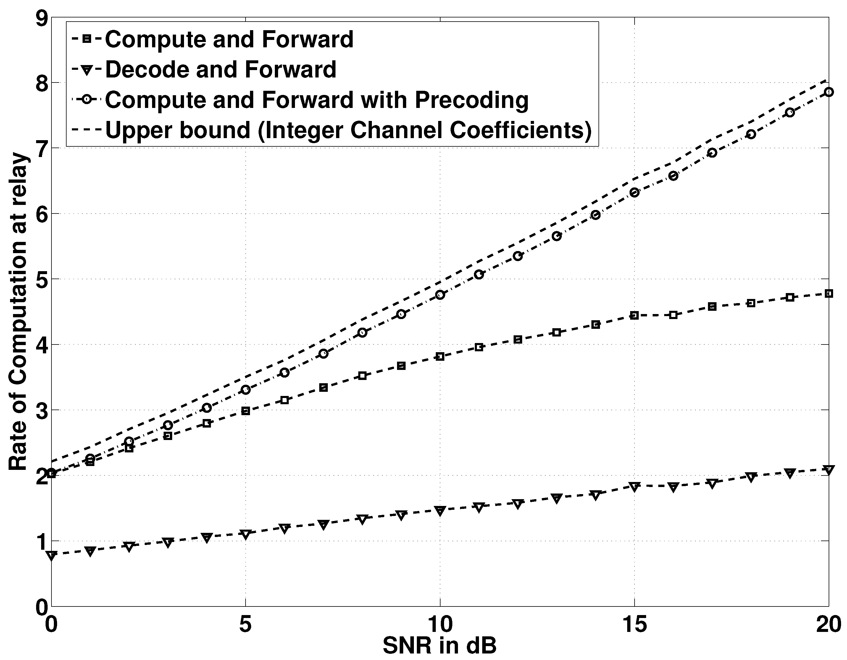
6.3. Achievable Rates

In this subsection, we compare the theoretical rates achieved by IFP in Equation (22) with existent schemes. We consider the rates achieved by three other schemes: (i) the decode and forward scheme, which requires decoding the original signals at the relay; (ii) the compute and forward scheme without precoding; and (iii) compute and forward obtained by considering integral channels, which serves as an upper bound for achievable rates in CF. For fair comparison, we have adjusted the total power available at the transmitters in all the schemes to be equal to ${\gamma }_x=\max \left({\gamma }_w\right)$. The channel gains, h= [$h_1$ $h_2$], are approximated by integers, a = [$a_1$ $a_2$]. The $log$ is taken to the base of two. The rates are measured in bits per channel use (bpcu). For decode and forward, the relay decodes one of the signals, treating the other signal as noise. Hence:

$$R_{DF}={\log }^{+}\left(\frac{{\gamma }_x\mid h_1{\mid }^2}{{\sigma }^2+{\gamma }_x\mid h_2{\mid }^2}\right)$$

For compute and forward without precoding, the relay computes the linear combination of original signals, and the non-integer part of the channel contributes to additional self-noise. The achievable rate is given by:

$$R_{CF}={\log }^{+}\left(\frac{{\gamma }_x\parallel \mathbf{a}{\parallel }^2}{{\sigma }^2+{\gamma }_x(\parallel \mathbf{h}-\mathbf{a}{\parallel }^2)}\right)$$

The upper bound of CF is computed considering the channels as integers ($\mathbf{h}=\mathbf{a}$) in which no additional self-noise is present. The rate achieved is given by:

$$R_{CF}^u={\log }^{+}\left(\frac{{\gamma }_x\parallel \mathbf{a}{\parallel }^2}{{\sigma }^2}\right)$$

We compare these rates with the rates for our proposed scheme. Figure 5 shows the achievable rates of different schemes for varying SNR. Clearly, the proposed implementation approaches the upper bound at high SNRs. The CF scheme without precoding suffers from increased self-noise as the signal power increases.

Figure 5. Comparison of achievable rates for various schemes for $L=2$. The average value is taken over 10,000 different random channel realizations. The rates are measured in bits per channel use (bpcu).

Figure 5. Comparison of achievable rates for various schemes for $L=2$. The average value is taken over 10,000 different random channel realizations. The rates are measured in bits per channel use (bpcu).

7. Conclusions

In this paper, we have proposed a novel scheme to implement the fundamental concept of CF. We have proposed an integer forcing precoder to precode the signals, such that the signal obtained at the relay is naturally a linear combination of original signals. The IFP effectively reduces the channel into an AWGN channel. The proposed scheme can remove the self-noise, which arises in CF, due to the approximation of the channel by an integer, but it incurs the penalty of extra power usage at the transmitter. We have shown that this extra power used is in a finite range for most channels.

Further, we have made an end-to-end analysis of the CF scheme by observing the performance of CF at the destination. The aim of the destination is to decode the original source signals from the linear combinations obtained from the relay. We have provided a two level decoding at the destination: firstly, the destination decodes the linear combinations from the noisy signal sent from the relay. Secondly, after obtaining L such linear combinations, the destination obtains the original source signals using the linear combinations.

To analyze the performance of our proposed scheme, we have also derived the expression for probability of error of the proposed scheme. We have also compared our proposed scheme to the existent schemes using numerical simulations. To this end, we have obtained the performance of the proposed scheme at the relay, as well as at the destination, making an absolute end-to-end analysis. We have used Bezout’s theorem to derive a closed-form expression for probability of error for the case of cubic lattices. In addition, we have also demonstrated the outage formulation of the proposed scheme, which arises due to the use of extra power at the transmitters. Concluding the analysis, we study the performance of IFP in terms of achievable rates and show that the use of channel state information at transmitters to design IFP helps attain considerable gains in terms of rates over traditional relaying scheme, like decode and forward.

CF is a natural transmission framework for upcoming vehicular networks. Achieving practically the theoretical limits of performance in such networks is a challenge, and CF is a promising approach to improve this performance. The precoder introduced in this work can be optimized according to specific scenarios, and such designs are required to be explored further.

References

- Zhang, S.; Liew, S.; Lam, P. Physical Layer Network Coding. 2006. arXiv.org Website. Available online: http://arxiv.org/abs/0704.2475 (accessed on 12 August 2013).
- Nazer, B.; Gastpar, M. Compute and forward: Harnessing interference through structured codes. IEEE Trans. Inf. Theory 2011, 57, 6463–6486. [Google Scholar] [CrossRef]
- Feng, C.; Silva, D.; Kschischang, F. An Algebraic Approach to Physical-Layer Network Coding. In Proceedings of 2010 IEEE International Symposium on Information Theory Proceedings (ISIT), Austin, TX, USA, 13–18 June 2010.
- Niesen, U.; Whiting, P. The degrees of freedom of compute-and-forward. IEEE Trans. Inf. Theory 2012, 58, 5214–5232. [Google Scholar] [CrossRef]
- Belfiore, J.-C. Lattice Codes for the Compute-and-Forward Protocol: The Flatness Factor. In Proceedings of the IEEE Information Theory Workshop (ITW), Paraty, Brazil, 16–20 October 2011; pp. 1–4.
- Nazer, B.; Gastpar, M. Reliable physical layer network coding. Proc. IEEE 2011, 99, 438–460. [Google Scholar] [CrossRef]
- Chen, F.; Silva, D.; Kschischang, F.R. Blind Compute-and-Forward. In Proceedings of the IEEE International Symposium on Information Theory Proceedings (ISIT), Cambridge, MA, USA, 1–6 July 2012; pp. 403–407.
- Hong, S.-N.; Caire, G. Reverse Compute and Forward: A Low-Complexity Architecture for Downlink Distributed Antenna Systems. In Proceedings of the IEEE International Symposium on Information Theory Proceedings (ISIT), Cambridge, MA, USA, 1–6 July 2012; pp. 1147–1151.
- Yang, T.; Yuan, X.; Li, P.; Collings, I.B.; Yuan, J. A new physical-layer network coding scheme with eigen-direction alignment precoding for mimo two-way relaying. IEEE Trans. Commun. 2013, 61, 973–986. [Google Scholar] [CrossRef]
- Gupta, S.; Vazquez-Castro, M.A. Physical-Layer Network Coding based on Integer-forcing Precoded Compute and Forward. In Proceedings of the IEEE 8th International Conference on Wireless and Mobile Computing, Networking and Communications (WiMob), Barcelona, Spain, 8–10 October 2012; pp. 600–605.
- Wiesel, A.; Eldar, Y.; Shamai, S. Zero-forcing precoding and generalized inverses. IEEE Trans. Signal Process. 2008, 56, 4409–4441. [Google Scholar] [CrossRef]
- Hassibi, B.; Vikalo, H. On the sphere-decoding algorithm I. Expected complexity. IEEE Trans. Signal Process. 2005, 53, 2806–2818. [Google Scholar] [CrossRef]
- Zamir, R. Lattices are Everywhere. In Proceedings of the Information Theory and Applications Workshop, San Diego, CA, USA, 8–13 February 2009; pp. 392–421.
- Forney, G.D., Jr. Coset codes-I: Introduction and geometrical classification. IEEE Trans. Inf. Theory 1988, 34, 1123–1151. [Google Scholar] [CrossRef]
- Monteiro, F.A.; Wassell, I.J. Dual-Lattice-Aided MIMO Detection for Slow Fading Channel. In Proceedings of the IEEE International Symposium on Signal Processing and Information Technology, Bilbao, Spain, 14–17 December 2011; pp. 502–507.
- Tarokh, V.; Vardy, A.; Zeger, K. Universal bound on the performance of lattice codes. IEEE Trans. Inf. Theory 1999, 45, 670–681. [Google Scholar] [CrossRef]
- Shub, M.; Smale, S. Complexity of Bezout’s theorem. I. Geometric aspects. J. Am. Math. Soc. 1993, 6, 459–501. [Google Scholar] [CrossRef]
- Papoulis, A. Probability, Random Variables, and Stochastic Processes, 2nd ed.; McGraw-Hill: New York, NY, USA, 1984; p. 104. [Google Scholar]
© 2013 by the authors; licensee MDPI, Basel, Switzerland. This article is an open access article distributed under the terms and conditions of the Creative Commons Attribution license (http://creativecommons.org/licenses/by/3.0/).
Share and Cite
Gupta, S.; Vázquez-Castro, M.A. Physical Layer Network Coding Based on Integer Forcing Precoded Compute and Forward. Future Internet 2013, 5, 439-459. https://doi.org/10.3390/fi5030439
Gupta S, Vázquez-Castro MA. Physical Layer Network Coding Based on Integer Forcing Precoded Compute and Forward. Future Internet. 2013; 5(3):439-459. https://doi.org/10.3390/fi5030439
Chicago/Turabian StyleGupta, Smrati, and M. A. Vázquez-Castro. 2013. "Physical Layer Network Coding Based on Integer Forcing Precoded Compute and Forward" Future Internet 5, no. 3: 439-459. https://doi.org/10.3390/fi5030439