Optimization of Vehicular Trajectories under Gaussian Noise Disturbances

Abstract

Nowadays, research on Vehicular Technology aims at automating every single mechanical element of vehicles, in order to increase passengers’ safety, reduce human driving intervention and provide entertainment services on board. Automatic trajectory tracing for vehicles under especially risky circumstances is a field of research that is currently gaining enormous attention. In this paper, we show some results on how to develop useful policies to execute maneuvers by a vehicle at high speeds with the mathematical optimization of some already established mobility conditions of the car. We also study how the presence of Gaussian noise on measurement sensors while maneuvering can disturb motion and affect the final trajectories. Different performance criteria for the optimization of such maneuvers are presented, and an analysis is shown on how path deviations can be minimized by using trajectory smoothing techniques like the Kalman Filter. We finalize the paper with a discussion on how communications can be used to implement these schemes.

1. Introduction and Motivation

According to statistics of the DGT (Spanish National Traffic Administration), around 91% of fatal traffic accidents take place on highways and conventional roads [1] in Spain. Up to 71% of these accidents occur due to the collision of two or more vehicles in transit, against a suddenly appearing obstacle on the road, or because of pedestrians or animals running over. This information shows how relevant it is to develop new technologies that can assist the driver or make autonomous decisions to increase passengers’ safety.

In this regard, the automotive industry is currently moving towards the automation of every single aspect of the driving experience [2]. The main trend, before cars are fully automated, consists of improving the driver assistance by providing new mechanisms that can increase safety and comfort. This can be effectively implemented by the installation of devices that can monitor the environment continuously and, at the same time, determine under which situations the driver needs some kind of specific aid (through somewhat advanced smart processing applications). By monitoring the environment, we mean using specific cameras and/or sensors that can acquire useful data to improve the driving experience.

Communications will also play an important role when disseminating information monitored by sensors installed on board to enhance the safety conditions of passengers while driving. The standard WAVE 1609/802.11p [3] has been designed for this purpose, and it covers the general communication schemes that vehicles will implement in to support V2V (vehicle to vehicle) and V2I (vehicle to infrastructure) communications. Through the use of communications, the amount of information that a car may process is much higher, and thus, with a proper processing scheme, it can be really useful to make timely and smarter decisions that would not be possible when isolated. Therefore, by using such technologies, vehicles could benefit from the environmentally collected data to take autonomous actions in order to reduce the probability of a fatal event (vehicle-vehicle collision, pedestrian/animal running over) at high speed.

Within this topic, a very concerning problem is how to perform the best emergency maneuvers. Interest in this issue has increased in the last decades [4], resulting in methods to find optimal trajectories for different objectives, mainly focused on single vehicles. However, emergency maneuvers should be planned by taking into account surrounding vehicles for obvious reasons. The deployment of vehicular communications paves the way for the development of methods to compute optimal trajectories for a set of involved vehicles. This is certainly a challenging goal. First, there are a wide number of possibilities to state the problem and select the appropriate functional to optimize. Second, either the problem may be solved in a distributed way or a leader car in a clustering scheme may solve it and deliver the solution to the remaining involved vehicles. A hybrid method entailing the exchange of independent solutions may be also suitable. Third, the variability to which the shape of trajectories might be subject (due to the disturbances in the controls that vehicles might suffer) makes it necessary to use mechanisms to correct the possible deviations from the optimum trajectory while maneuvering to reduce the negative influence of undesirable phenomena.

In the present study, we focus on the development of useful procedures to dynamically optimize the trajectory of a vehicle under timing constraints, i.e., changing its lateral position on the road to maximize the lateral distance within an interval of t_f . Additionally, we minimize some other mobility parameters like the lateral speed at the end of the path (to reduce the impact of sudden inertial changes). Finally, we carry out a study on how diversion from the optimum trajectory due to Gaussian noise in measurement sensors can be minimized thanks to the well-known the Kalman Filter technique [5]. Since this mathematical optimization framework will be extended for cooperative collision avoidance (CCA) in a future work, we also discuss how it can be implemented with our proposal. That is, we show here the results of a first step within our general goal, focusing on different functionals and providing useful insight on the resulting trajectories that can be expected from them, as well as a simple analysis on how noise disturbances can affect trajectories and possible solutions to this undesirable effect. In summary, the main contributions of this paper are:

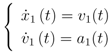
• A discussion on the different ways to compute optimized real-time maneuvers for a high-speed moving vehicle subject to timing constraints (the maneuver must be performed in a maximum time interval of t_f ).
• The evaluation of functionals including the minimization of the final lateral speed. By keeping the final lateral speed (at t_f ) as low as possible, the possibility of continuing in the optimum lateral position is also maximized.
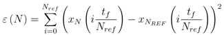
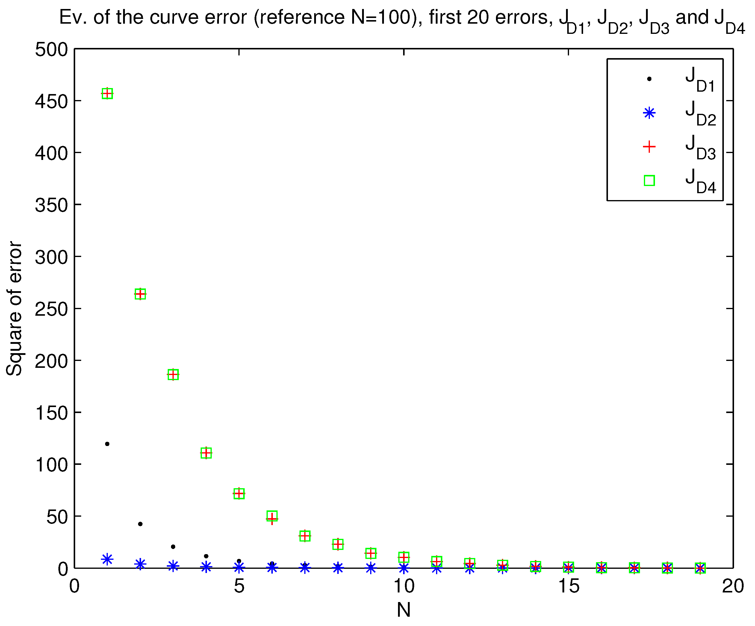
• A preliminary discussion on the accuracy of the computed trajectories by an evaluation of the discretization factor N (number of stages in which the trajectory is divided into).
• An analysis on how trajectories could be affected by random Gaussian noise, and the application of Kalman Filter theory to minimize the impact of unwanted deviations from the optimum path.

The rest of this paper is organized as follows. In Section 2 the reader will find some previous related work that served as a reference for the development of our proposal. Section 3 will state the problem’s most important features and different illustrative results to evaluate the performance of our trajectory tracing algorithm. This section will be finalized with the aforementioned study on optimum path recovery by means of the Kalman Filter. Section 4 will conclude the paper with some important remarks and pointing out our future work.

2. Related Work

Several previous studies on active maneuvering not directly related to emergency maneuvers can be found in the open literature. In the case of [6], we can find a mathematical evaluation in which some interesting properties of active maneuvering are obtained by applying Optimal Control theory (OC) to the calculation of optimum trajectories in order to obtain a given final heading. Satisfying either minimum time or minimum distance, the results in [6] showed that trajectory tracing for just one vehicle when looking for a specific heading can be useful when dealing with general robots, but not as much when talking about vehicles, which essentially would expect to avoid an accident, regardless of the final heading. In [7] the authors proposed an approach to solve the problem of tracing the trajectory for a car between two fixed points. This type of problem is a BVP (Boundary Value Problem) in which the main concern is to study the trajectory between two fixed points while optimizing the time employed to complete this trajectory according to some physical constraints in terms of maximum acceleration. This evaluation gave a useful hint on the analysis of OC problems by providing a mathematical functional based on nearly-time optimality for the solution of the problem. However, this formulation of the problem suffers from convergence issues as well as tight constraints in values for mobility parameters (such as speed). Furthermore, fixed final boundaries are rarely met under real circumstances due to the obvious variability of the environmental conditions. Another approach for the establishment of an optimal control law for a pair of Dubin’s vehicles (cars moving characterized by a sinusoidal differential equations model) is found in [8], where authors obtain trajectories that transfer the two Dubin’s vehicles from pre-established initial positions to fixed final locations in space. The optimization goals in [8] included the minimization of acceleration, speed and distance along the trajectory and the maximization of the distance between the two vehicles during the maneuver. This is essentially a BVP where there is some sort of cooperative trajectory optimization. A more closely related work is found in [4], where the collision avoidance problem is formulated as an IVP (Initial Value Problem) in which a vehicle divides the trajectory tracing procedure into three stages (each one with its own functional). The first one consists of steering to simply avoid the collision against the obstacle; the second phase affords the reorientation of the trajectory to avoid colliding against the lateral protections; and the last one deals with relocating the car in the same lane it was circulating before. Moreover, this work provided a realistic mobility model of the vehicle. In fact, the goal of the paper was to study the advantages of additional actuated degrees of freedom. According to general path planning techniques, we find in the literature some important works regarding online trajectory tracing by using fuzzy logic. That is the case of the research led by Naranjo in [9], where a power-steering control architecture for autonomous driving is proposed. Integrated into two different layers (target position calculation and vehicle positioning), the offered architecture showed by experimentation that the combination of different sensing sources (GPS, vision...) by artificial intelligence provides a reliable behavior of the car in transit. Another work of the same authors was presented in [10], where the associated AUTOPIA architecture was introduced in detail, including the recent advances in terms of specific car maneuvers designed for autonomous car control in such vehicles.

3. Problem Statement and Results

In this section we start giving a description of the specific problem we tackle in this evaluation, formulating the problem, discussing alternative functionals and describing the tools used to solve it. We will also analyze the performance of the trajectory tracing procedure and how we can address the inconvenience of path deviations because of additive noise processes affecting sensor measurements while maneuvering. We conclude this section by providing a qualitative analysis of the connection between our proposal and how it might be integrated within some sort of vehicular networking protocols.

3.1. Scenario Description and Formulation

The general problem we are interested in deals with computing a trajectory tracing procedure to handle critical situations under which a vehicle circulating at high speeds has to avoid the collision against a suddenly appearing obstacle (another vehicle, a pedestrian or an animal) in the middle of the road.

However, we think it is instructive to examine in detail alternative formulations, thus in this paper we will focus on the simplest version of the problem in order to get an understanding on how trajectories for a single vehicle evolve according to the specific optimization requirements we set, and how the behavioral restrictions to which the car’s mobility is constrained affect the maneuver. As a straightforward version of the problem, we assume there is only one vehicle circulating on a W-meter-wide road (regardless of the number of lanes). This vehicle has to trace a trajectory in an interval of t_f seconds after the maneuver has begun (see Figure 1). During this interval, the vehicle will try to adjust its mobility evolution according to a set of constraints and optimizing a given functional. In this particular case, our goal would be to achieve a given degree of safety while keeping the maneuver as comfortable as possible. To combine these two features, we look for the maximization of the lateral distance with respect to the lateral boundaries of the road, while minimizing the final lateral speed at the end of the path, all within a given time interval of t_f seconds. Maximizing the lateral distance implies in this case leaving the maximum possible road width on both sides of the vehicle, thus minimizing the probability of colliding with the lateral protections. On the other hand, by simultaneously minimizing the lateral speed at t_f , we can change the general appearance of the trajectory in such a way that the inertial impact on the mobility of the passengers is reduced when reaching the optimum lateral position.

Figure 1. Maximization of lateral distance after t_f .

Figure 1. Maximization of lateral distance after t_f .

For the analysis of the problem, we first need to assume a model for the vehicle’s motion, which is represented by the system of differential equations that describes the lateral movement of the car (only x axis, see Figure 1):

(1)

where x₁(t) refers to the position of vehicle 1 in axis x at time t; v₁(t) denotes the current speed of vehicle 1 in axis x as a function of t; and a₁(t) defines the lateral acceleration of vehicle 1 along time. We take a₁(t) as the control variable that we have to manipulate in real time in order to modify the trajectory traced by the vehicle under consideration. As was specified before, we assume that these mobility equations only govern the lateral displacement of the vehicle (we consider the longitudinal speed to be constant and fixed to 120 km/h during the whole trajectory).

Furthermore, the car’s mobility has to respect the physical limits imposed by the inertial laws of kinematics. This means that the vehicle can only turn at a maximum established acceleration, which depends on the longitudinal speed (the higher the speed, the harder the maneuver). Considering this, we can establish the mechanical restrictions of the problem at hand:

• Lateral acceleration restrictions. The absolute value of the lateral acceleration cannot take a value higher than the limit c(vi) m/s², where vi is the constant longitudinal speed of the vehicle and c(·) is a function of the longitudinal speed.

  (2)
• Lateral position restrictions. The vehicle can only have a lateral displacement inside the width limits of the road.

  (3)

The third and most important aspect of the statement of the problem is the functional we want to optimize. Although it is possible to formulate different functionals according to the specific target we want to optimize, we will focus on just the previously mentioned main objectives: minimization of the variance of the lateral distance (as we will see, by minimizing the lateral variance of the distances we simultaneously maximize lateral distance), and minimization of the final lateral speed. As we said, this can be justified due to the fact that the lower the variance of the distances of the lateral gaps (between two vehicles, two obstacles or vehicle to obstacle), the higher the lateral distance to other elements on the road will be. On the other hand, minimizing the final lateral speed will turn into a null lateral inertia when approaching the end of the path as we will see later.

Even though we restrict ourselves to these parameters, alternative functionals can be constructed. The four proposed functionals are described next:

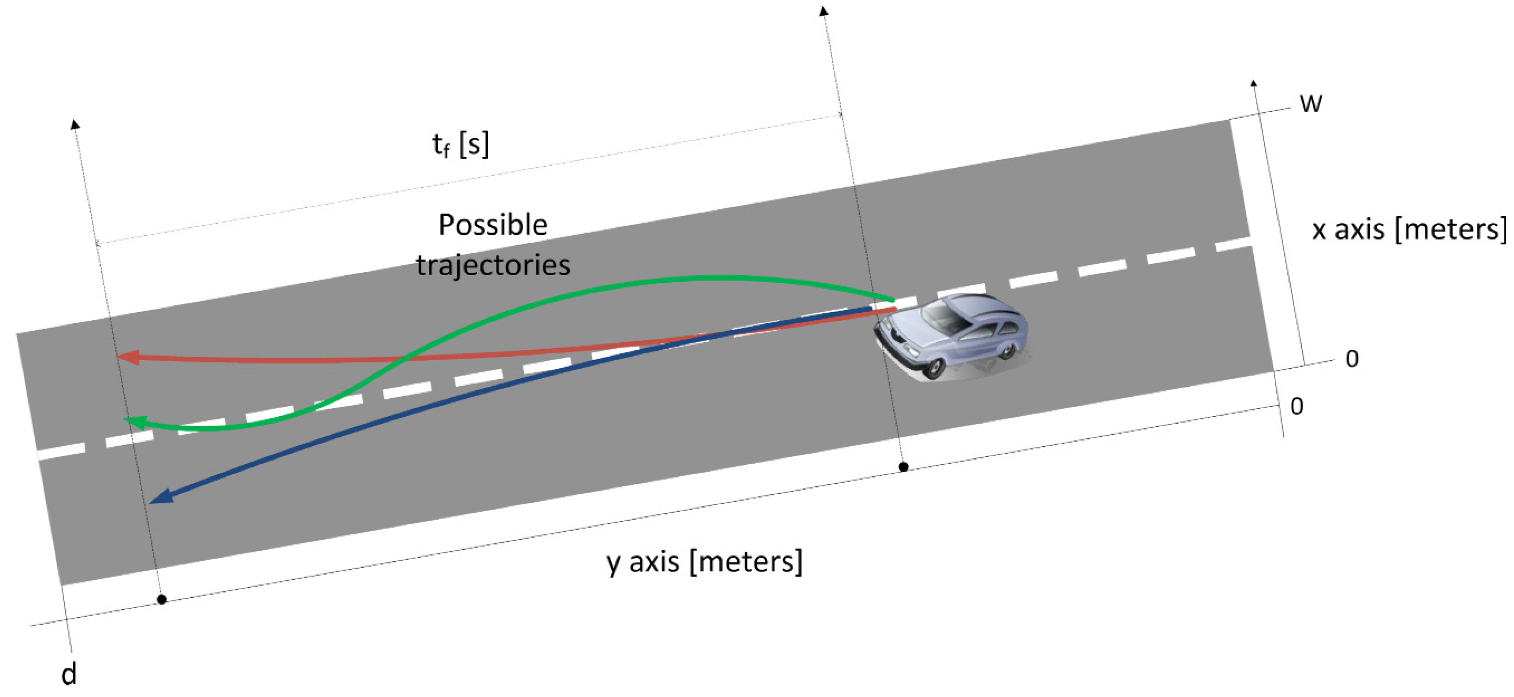
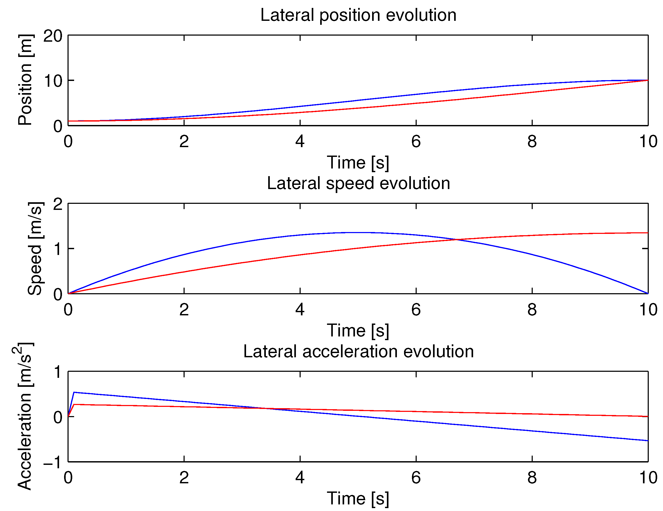
• Final lateral distance maximization and final lateral speed minimization. In this case we want to minimize the final variance of the lateral distances left by the vehicle after t_f , while minimizing the lateral speed at the end of the trajectory. The equation corresponding to this functional takes the form:

  (4)
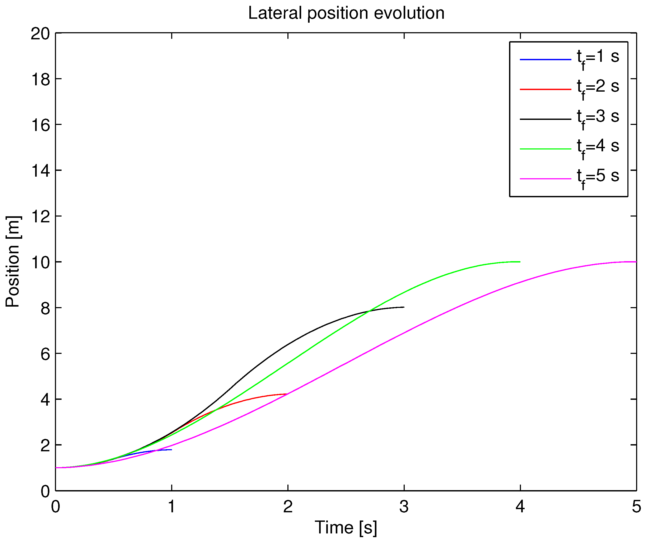
• Final lateral distance maximization. In this case we skip the minimization of the lateral speed at the end of the trajectory. We only perform here the maximization of the final lateral distance.

  (5)
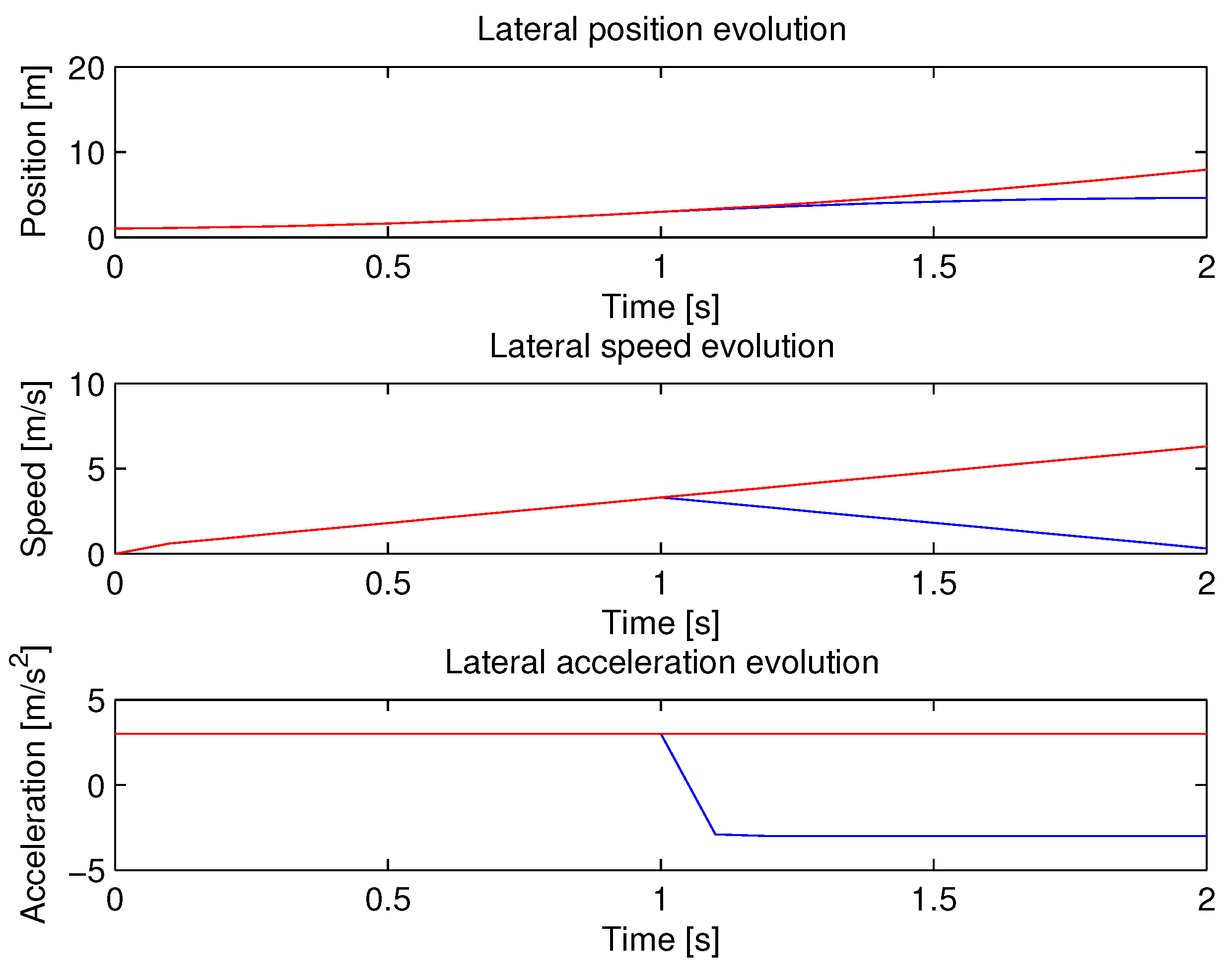
• Instantaneous lateral distance maximization and final lateral speed minimization. This functional aims at maximizing the instantaneous lateral distance while minimizing the lateral speed at the end of the trajectory.

  (6)
• Instantaneous lateral distance maximization. In this case, we skip the minimization of the lateral speed at the end of the trajectory, but we maximize the instantaneous lateral distance (during the maneuver).

  (7)

For the optimization of the aforementioned functional, we will rely on the Gradient Projection Algorithm, a class of Gradient Descent procedure that includes functionals that can only be optimized inside a region determined by the constraints of the problem [11]. This method requires to discretize the trajectory into N steps. Apart from the evaluation of trajectories, in the next subsections we will explore how the discretization factor N influences on the determination of trajectories and the resolution we need according to the specific functional in order to reach a reasonable trade-off between curve error and computational load.

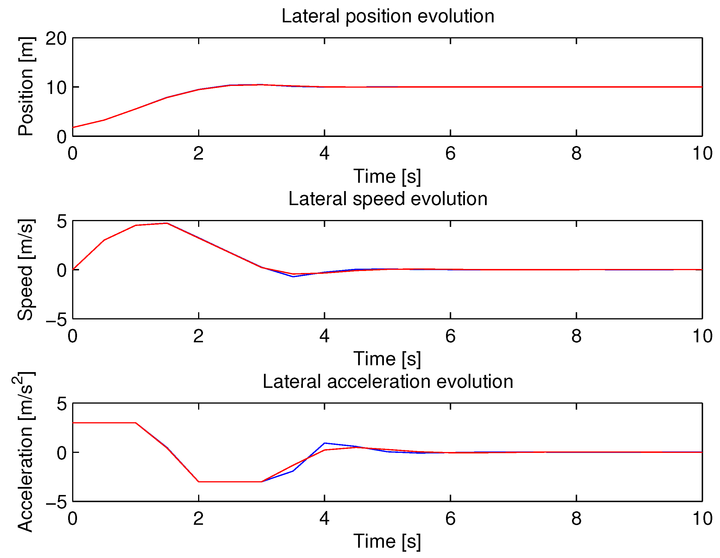
3.2. Final Lateral Distance Maximization

In this first subsection, we compare the performance of functionals J_D1 and J_D2 for the configuration of parameters in Table 1, where the instantaneous lateral distance of the vehicle along the trajectory is not maximized, but the final (at t_f ) lateral distance to the lateral protections is maximized. If we obtain the mobility evolution (acceleration, speed and position evolution along the trajectory) for two different values of t_f (10 and 2 seconds), we can notice from Figure 2 and Figure 3 that for longer time intervals to execute the maneuver, the vehicle does not need to reach the maximum acceleration stated by the model’s restrictions. On the other hand, for lower values of t_f , the steering maneuver needs to use the maximum allowable values of the lateral acceleration to maximize the functional at the end of the trajectory. The most illustrative differences between both functionals can be read from Figure 2 and Figure 3, where we see that J_D1 (blue) reaches a higher lateral peak speed than J_D2 just at the middle of the time period. The explanation for this fact is that by flipping between two opposite values of the acceleration (see Figure 2 and Figure 3) until the final position is reached, the vehicle can get there with null lateral speed. However, for J_D2, the speed will increase more smoothly from the first instant, but at the cost of not having null lateral speed at the end of the trajectory, which could lead to a further potential risk because of the inherent inertial dynamics.

Table 1. Configuration parameters and values for all evaluations.

Evaluation parameter	Meaning	Value
N	Discretization factor	20
X0	Initial lateral position	1 m
V0	Initial lateral speed	0 m/s
a0	Initial lateral acceleration	0 m/s2
W	Road width	20 m
vi	Longitudinal speed	120 km/h
c(vi)	Maximum absolute lateral acceleration	3 m/s2

Table 1. Configuration parameters and values for all evaluations.

Evaluation parameter	Meaning	Value
N	Discretization factor	20
X0	Initial lateral position	1 m
V0	Initial lateral speed	0 m/s
a0	Initial lateral acceleration	0 m/s2
W	Road width	20 m
vi	Longitudinal speed	120 km/h
c(vi)	Maximum absolute lateral acceleration	3 m/s2

Figure 4 and Figure 5 show the trajectories traced by the two functionals for different values of the final time (t_f ). Analyzing the results in these figures, we can conclude that functional J_D1 can reach the optimum lateral position at a later time but with a null lateral speed, whereas through functional J_D2 it is possible to reach the optimum lateral position earlier, but at the expense of having a non-zero speed. The first one will not have problems to follow the trajectory, but for the second one, safety relies on how will the inertial mobility be from the instant t_f onwards.

Figure 2. Position, speed and acceleration J_D1 (blue) and J_D2 (red) (t_f = 10 s).

Figure 2. Position, speed and acceleration J_D1 (blue) and J_D2 (red) (t_f = 10 s).

Figure 3. Position, speed and acceleration J_D1 (blue) and J_D2 (red) (t_f = 2 s).

Figure 3. Position, speed and acceleration J_D1 (blue) and J_D2 (red) (t_f = 2 s).

Figure 4. Trajectory evolution of functional J_D1 for different t_f .

Figure 4. Trajectory evolution of functional J_D1 for different t_f .

Figure 5. Trajectory evolution of functional J_D2 for different t_f .

Figure 5. Trajectory evolution of functional J_D2 for different t_f .

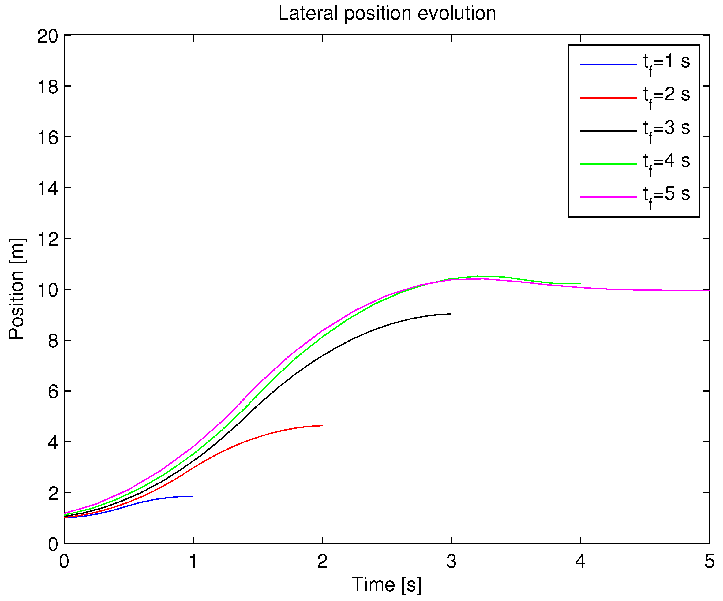
3.3. Instantaneous Lateral Distance Maximization

In this part, we focus on analyzing the properties of the trajectories when we use the instantaneous lateral distance maximization as the optimization target (J_D3 and J_D4). As we can infer from Figure 6 and Figure 7, in this case the main objective consists of updating the lateral position as soon as possible in order to meet the requirements set by the functionals.

Figure 6. Position, speed and acceleration J_D3 (blue) and J_D4 (red) (t_f = 10 s).

Figure 6. Position, speed and acceleration J_D3 (blue) and J_D4 (red) (t_f = 10 s).

Figure 7. Position, speed and acceleration J_D3 (blue) and J_D4 (red) (t_f = 2 s).

Figure 7. Position, speed and acceleration J_D3 (blue) and J_D4 (red) (t_f = 2 s).

This implies using alternatively the two highest (absolute) values of acceleration during the trajectory, which naturally makes the vehicle build a more sensitive path that can be obviously more affected by additional disturbances (i.e., bad weather conditions). This is explained by assuming that the vehicle will try to adapt its lateral position instantaneously in order to maximize the lateral distance. Thus, it is possible that if there is a sudden change in the width of the road, or another car gets too close, the trajectory is modified very harshly, so it could undoubtedly end in a lateral collision. With J_D1 and J_D2 there could effectively be lateral collisions, but they are less prone to disturbances, because lateral distance is maximized regarding only the final lateral positions.

Evaluating the results for the same scenario (see Table 1) for J_D3 and J_D4, we can see that for longer time intervals (Figure 8) until reaching the final position, a vehicle focus on achieving the final lateral position very quickly (thus the rapid changes in acceleration, which oscillate between the two extreme values although there is enough time to make a smoother maneuver). Besides, it is surprising that for both functionals the final lateral speed reached at the end of the path is null, and both functionals provide very similar behaviors. On the other hand, if we analyze Figure 9, we see that for very short time intervals, the evolution of mobility is very similar to what we saw for the functionals J_D1 and J_D2.

Figure 8. Trajectory evolution of functional J_D3 for different t_f .

Figure 8. Trajectory evolution of functional J_D3 for different t_f .

Figure 9. Trajectory evolution of functional J_D4 for different t_f .

Figure 9. Trajectory evolution of functional J_D4 for different t_f .

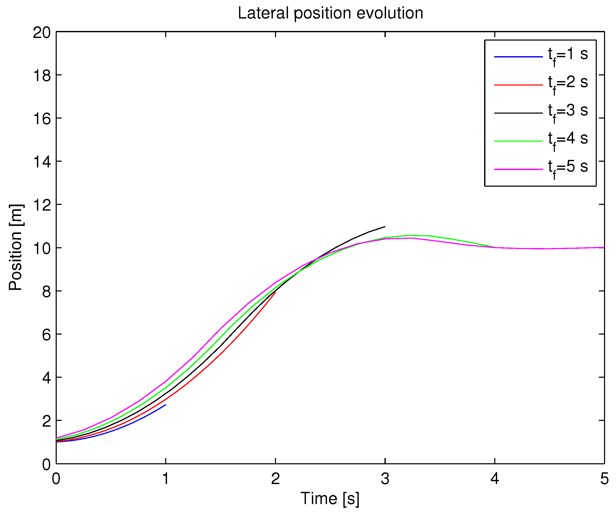
3.4. Discretization Influence

Considering that using Gradient Projection [11] to solve the optimization problems at hand implies the discretization of the trajectory in N steps (of constant acceleration), here we focus on the influence of the discretization factor N. We will compare here the trajectories traced by the four proposed functionals for a discretization factor N ∈ {1, ..., 20} and evaluate the error (as the sum of the square of the difference between one curve and the reference one, set to N = 100, see Equation 8). We consider the curve N = 100 as accurate enough for the calculation of the error evolution. The parameter configuration for this case is the same as for previous subsections (Table 1).

(8)

where ε(N) refers to the square error for an N-discretized curve x_N(t), in comparison with the N_ref = 100 reference trajectory x_Nref(t).

Having a look at the Figure 10, it is easy to realize the correctness of the trajectories calculated by the optimization algorithm (Gradient Projection), i.e., the highest errors are located for low values of the discretization factor, whereas the error value decreases as N gets higher.

Figure 10. Influence of discretization factor N.

Figure 10. Influence of discretization factor N.

Observing this graph, it is also straightforward to infer that setting a value of N = 20 should be enough to achieve a proper resolution in the curve for the four functionals. We can see that the functional J_D1 needs a higher value for the discretization factor than that of J_D2 to achieve the same level of accuracy. Due to the need of higher accelerations for the trajectories obtained by J_D1 in comparison with those calculated by J_D2, a higher value for the discretization factor N is thus required to keep an acceptable accuracy. On the other hand, both functionals regarding instantaneous lateral distance maximization (J_D3 and J_D4) show that they need a higher value of the discretization factor to reach the same level of accuracy. This is explained by the same reasons as regards the comparison between J_D1 and J_D2, that is, the greater acceleration values of the trajectories, the higher N must be to maintain accuracy.

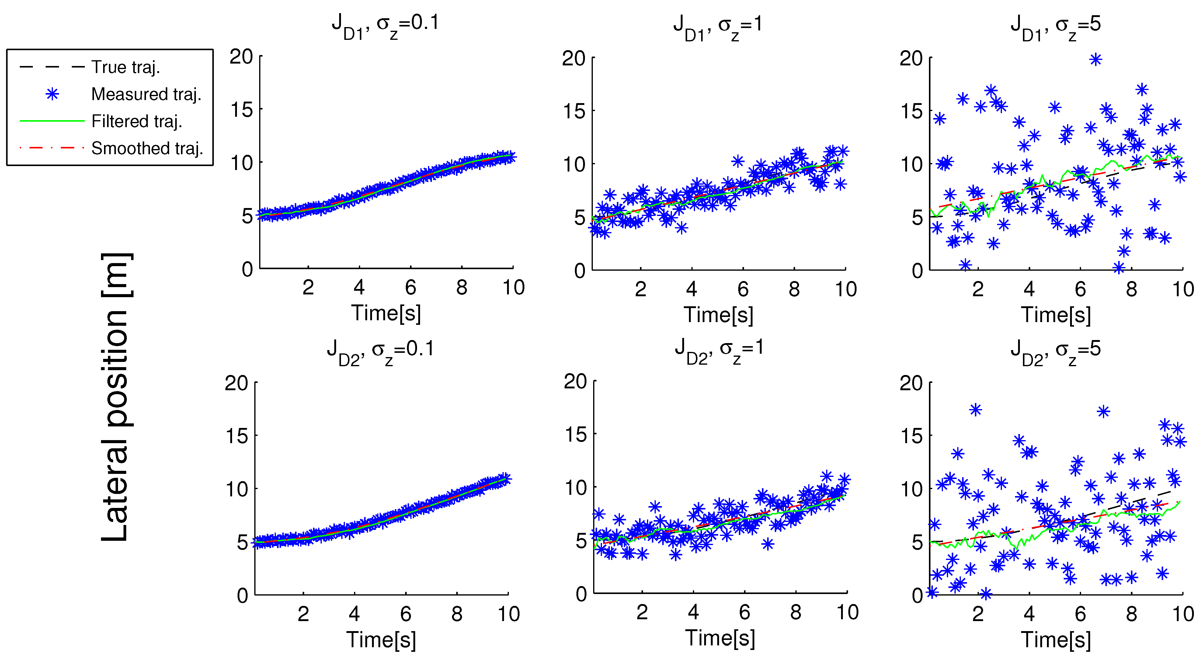
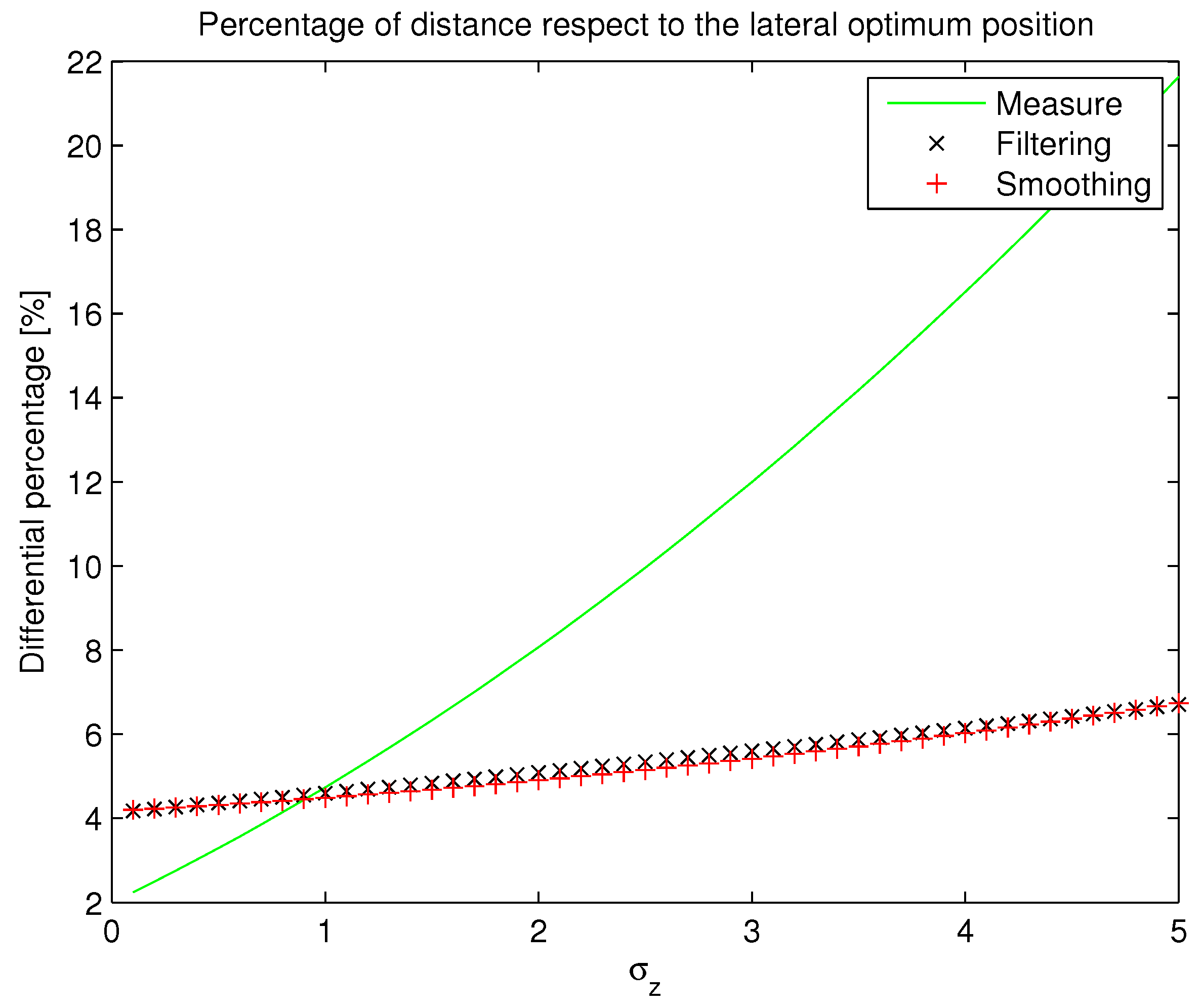
3.5. Kalman Filter for Trajectory Smoothing

Until now we have been dealing with the optimization of trajectories for a single vehicle according to two possible performance criteria. Needless to say, once the optimum trajectory is determined (here for the sake of simplicity, we disregard the time to compute the trajectories), the vehicle obviously start running the calculated path. In real cases, the vehicle will have to face undesirable phenomena during the maneuver’s execution, which could perturb the previously calculated optimum trajectory and make it divert from the calculated path. This is usually called the Random Noise Disturbances [12] in the literature. In this subsection we will extend the initial System of Equations describing the mobility of our one-dimensional vehicle to accomplish for this variability in the execution of the maneuvers. We will model such phenomena by assuming that an additive Gaussian noise process produces this variability by influencing:

• The shape of the traced path due to possible deviations from the optimum course, see Subsection 3.5.1.
• The sensors’ measurement on the position and speed at a fixed time t, see Subsection 3.5.2.

Kalman Filter theory has been proven to be a very reasonable option for state estimation and path reconstruction under the aforementioned circumstances. Moreover, it is the core technology that implements basic car localization and motion on autonomous vehicles, like the famous Google Car [13]. Before discussing in detail the characteristics of the Kalman Filter, we will first express our extended model for the System (1) by accounting for the two influencing factors presented earlier:

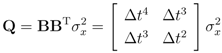
3.5.1. State Variability

The Kalman Filter model assumes the true state at time k is evolved from the state at (k − 1) as expressed by:

(9)

where F defines the state transition model applied to the previous state x (k − 1); B denotes the control-input applied to the controls u(k); w(k) is the process noise, which is assumed to be drawn from a zero mean multivariate normal distribution with covariance Q(k):

(10)

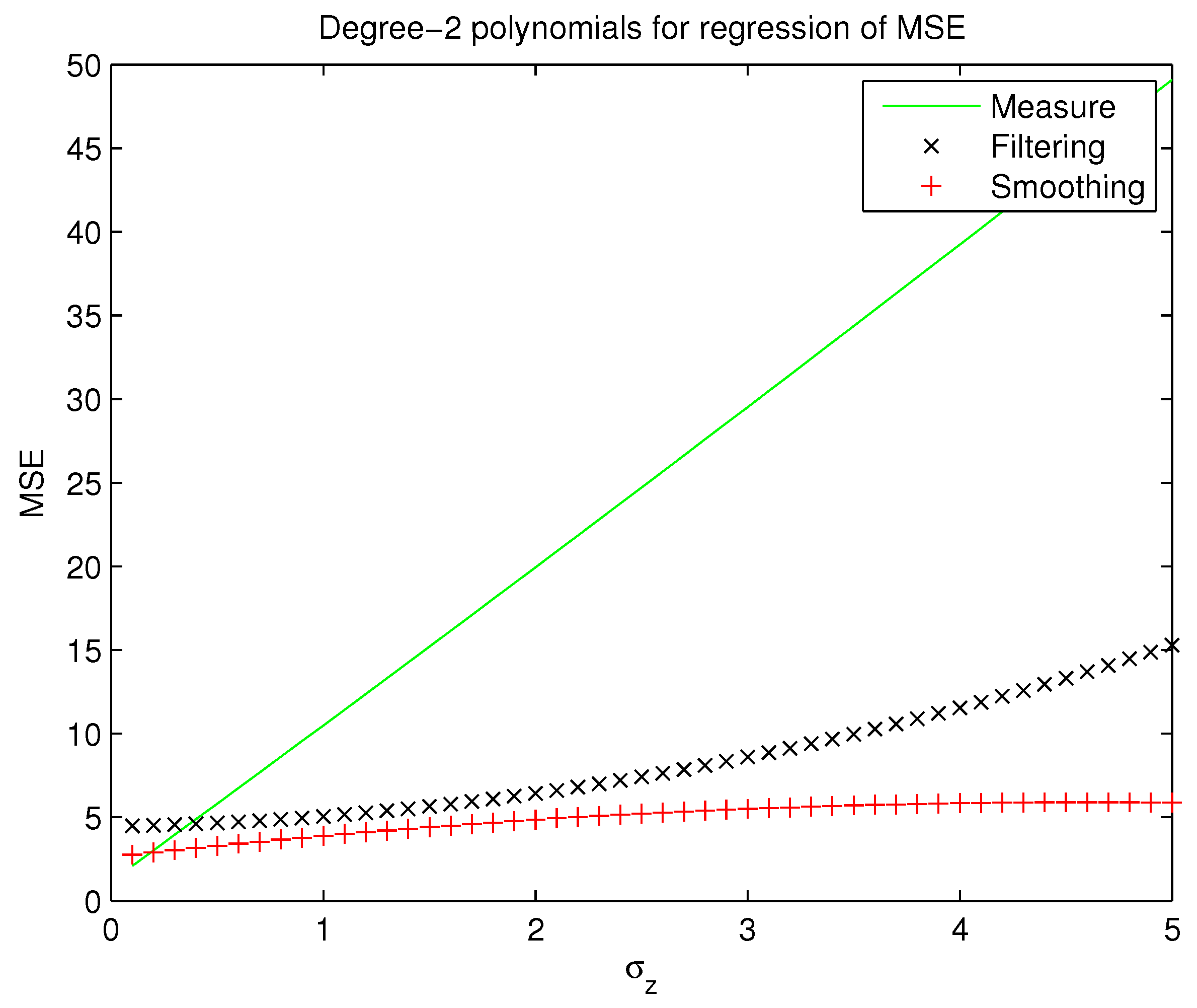
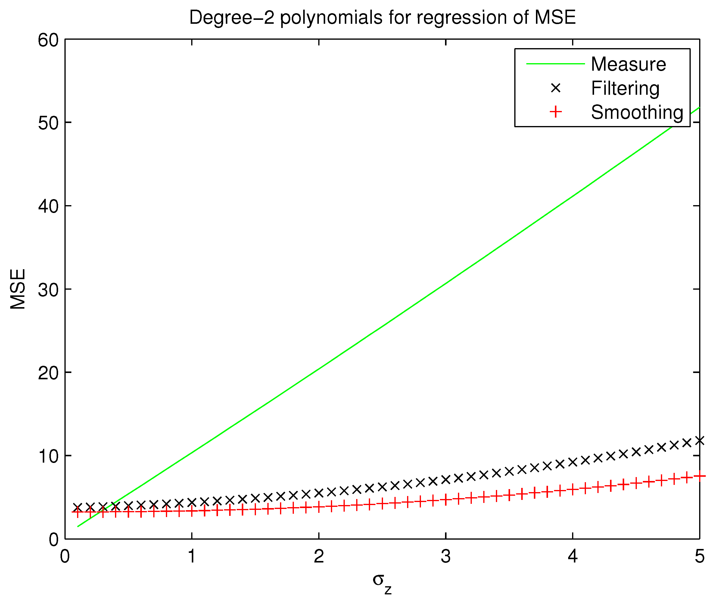
3.5.2. Measurements Variability

At time k an observation (or measurement) z (k) of the true state x (k) is made according to:

(11)

where H is the observation model that maps the true state space onto the observed space; and v (k) is the observation noise, which is assumed to be zero mean Gaussian white noise with covariance R(k):

(12)

We can observe that in comparison with the initial proposal of System (1), we now model our problem as a linear system of equations whose state variables are corrupted by additive Gaussian noise, represented by variable w(k) (Gaussian noise process of mean 0 and covariance Q(k), Equation (10)). Furthermore, we consider that there exists some sort of measurement sensing error, represented by variable v(k) (Gaussian noise process of mean 0 and covariance R(k), Equation (12)).

The position and speed in the extended System (9) is described by:

(13)

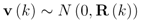
with being the derivative of lateral position with respect to time (speed v (k)).

Let us now express the F, B and H matrices by extracting the correspondence of both the controls and the state variables with Equations (10) and (12). After some easy operations we get:

(14)

Focusing on the covariance matrices regarding process and measurement noise, we get:

(15)

(16)

From this set of Expressions we are now capable of evaluating how different values of the measurement variance σ_z² and the state dispersion variance σ_x² affect the evolution of trajectories. With the Kalman Filter, it is possible to minimize the counterproductive effect of both noise processes by using two trajectory regeneration procedures enumerated next:

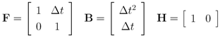
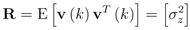
• Filtering. By means of this process, the Kalman Filter predicts the new values x (k) of the states taking into account the states’ history until the instant (k − 1). (Although the term “Kalman Filter” regards all techniques to reduce the influence of noise on the states of a dynamical system, we must not get confused with Filtering, which, as well as Smoothing, describes a specific procedure to fix or reduce trajectory dispersion caused by any noise process.)
• Smoothing. In this second process, the Kalman Filter estimates the new values x (k) of the states taking into account, apart from the states’ history until the instant (k − 1), the current measurement of the states: z (k).

We can deduce from the previous two comments that with Smoothing, the estimated trajectory will reduce the dispersion with respect to Filtering, since we count on more updated information to estimate the current position and speed of the vehicle.

Now it is time to graphically visualize some application examples of the previous concepts. In the first set of graphs, we will show how the trajectory of a vehicle (departing from a lateral position x = 5 m and having at most t_f = 10 s to reach the optimum lateral position) is affected by the presence of additive Gaussian noise in the states and in the sensor measurements. We will establish a state dispersion variance σ_x² = 0.1 for all the examples and will focus only on the influence of noise produced by measurement sensors (measurement variance σ_z²). We will include a comparison between the True Trajectory (optimum determined trajectory), the measured trajectory (sensed trajectory while executing the maneuver), and the filtered and smoothed trajectory for the two proposed performance measures J_D1 and J_D2, and for a set of values of the measurement variance σ_z² = {0.1, 1, 5}. If we now draw our attention to Figure 11, we can fairly understand how measurement noise affects the shape of trajectories by producing a dispersion of the optimum path due to the sensed positions along the course (mild dispersion for σ_z² = 0.1, medium dispersion for σ_z² = 1 and high dispersion for σ_z² = 5). We can notice that both Filtering and Smoothing reduce the dispersion effect, but Smoothing reduces the still significant variability that the filtered trajectory obtains, by using the measurement of the present instant z (k). Differences between J_D1 and J_D2, if present, are not clear in Figure 11.

Figure 11. Kalman filter effect on trajectories for J_D1 and J_D2 under measurement noise (σ_z = {0.1, 1, 5}).

Figure 11. Kalman filter effect on trajectories for J_D1 and J_D2 under measurement noise (σ_z = {0.1, 1, 5}).

Now we turn our attention to the evaluation of the Mean Square Error (MSE) between the optimum trajectory, and the measured, filtered and smoothed trajectories for the interval σ_z² ∈ [0,5], for both J_D1 and J_D2. Due to the variability to which the MSE is subject, we have used regression techniques to represent the Degree-2 polynomial, which averages the MSE evolution during the evaluated interval. This will make the visualization of graphs easier for comparison purposes.

On the other hand, we will also represent the averaged evolution (with a Degree-2 polynomial like with MSE) of the lateral distance with respect to the optimum lateral position (which we call LDP) at the last time step t_f in order to quantify how far the trajectory ends from the desired position. The associated graph will represent this magnitude for the same interval σ_z² ∈ [0,5] as in the last case, and will show the percentage, with respect to the total width of the road W , of distance far from the optimum lateral position.

If we have now a look at Figure 12 and Figure 13, we will see the evolution of both the MSE and LDP for the functional J_D1.

Figure 12. Degree-2 polynomials for regression of MSE under measurement noise (σ_z ∈ {0.1, 1, 5}), for J_D1.

Figure 12. Degree-2 polynomials for regression of MSE under measurement noise (σ_z ∈ {0.1, 1, 5}), for J_D1.

Figure 13. Percentage of distance with respect to the lateral optimum position under measurement noise (σ_z ∈ {0.1, 1, 5}), for J_D1.

Figure 13. Percentage of distance with respect to the lateral optimum position under measurement noise (σ_z ∈ {0.1, 1, 5}), for J_D1.

For the MSE, we can notice that for lower values of the measurement variance σ_z ∼ 0.1, sensing noise does not affect the trajectory remarkably, since the measured, filtered and smoothed paths obtain a very low MSE with respect to the optimum trajectory. As σ_z increases, it is easily noticeable how necessary it is to use at least Filtering and, if possible, Smoothing in order to correct the path dispersion introduced by noise. Surprisingly, the LDP shows very similar results for both Filtering and Smoothing, since both tend to reach the optimum final position regardless of the evolution of the trajectory. Analyzing now Figure 14 and Figure 15, we can come to the same conclusions as for the J_D1 functional. More importantly, we can see that differences between using Filtering and Smoothing for J_D1 and J_D2 are not as remarkable. This implies that the shape of the traced trajectory does not influence the performance of the Kalman filter.

Figure 14. Degree-2 polynomials for regression of MSE under measurement noise (σ_z ∈ {0.1, 1, 5}), for J_D2.

Figure 14. Degree-2 polynomials for regression of MSE under measurement noise (σ_z ∈ {0.1, 1, 5}), for J_D2.

Figure 15. Percentage of distance with respect to the lateral optimum position under measurement noise (σ_z ∈ {0.1, 1, 5}), for J_D2.

Figure 15. Percentage of distance with respect to the lateral optimum position under measurement noise (σ_z ∈ {0.1, 1, 5}), for J_D2.

3.6. Connection to Cooperative Collision Avoidance (CCA)

Analyzing the procedure of automatic trajectory tracing for one vehicle is the first step to completely evaluate a traffic scenario where vehicles interchange information to update their trajectories in common while simultaneously adapting to the unpredictable phenomena that could alter the normal transit. Even though we have not considered a real cooperative system, the previous discussion provides us with a valuable insight into the performance of alternative functionals for optimum trajectories. In the context of CCA, the proposed method involves the exchange of computed trajectories at discretization steps, or at least updated information that would require a high frequency of beacons’ interchange between vehicles in order to keep an updated history of the evolution of cars along the path. The IEEE 802.11p [3] is based on a CSMA (Carrier Sense Multiple Access), a medium access technique whose performance degrades as the number of transmitting nodes increases [14]. Thus, it is important to determine which are the minimum requirements that this system should have in order to guarantee appropriate performance (necessary in situations in which having this kind of information is critical). It might also be interesting to study the 3GPP/LTE (next generation, 4G) cellular infrastructure, which is already under deployment, in order to complement such technologies to properly relieve WAVE-based communications from the channel overload that V2I and V2V might entail [15]. This is something we will treat in a future work.

4. Conclusions

In this paper, we have discussed how to trace the optimum trajectory of a high speed vehicle that wants to relocate its lateral position before a time interval of t_f . We have proposed and evaluated four different functionals and discussed their advantages and drawbacks. Functionals J_D1 and J_D2 provide a better stability during the trajectory because they only update the mobility parameters according to the final lateral position. J_D3 and J_D4, however, are based on updating the lateral position in terms of the instantaneous distance, which requires faster changes in the mobility evolution. On the other hand, whereas J_D1 is really useful for higher values of t_f (since apart from reaching the optimum position it arrives with null lateral speed), J_D2 reaches the last position with a speed always higher than zero. However, for low distances until the optimum position (i.e. low values of t_f ), J_D2 can get to this position earlier, while the other functional focuses its attention on reaching the last position at zero speed, not caring as much about how far is the vehicle from the optimum position. From these results, we can deduce that in general optimizing in terms of the final lateral distance can be better to avoid very rapid changes in acceleration, which could imply the need to have higher values for the discretization factor N (at the expense of more computation overhead). However, we have not explored the great multiplicity of scenarios that appears from this premise, therefore using functionals J_D3 and J_D4 (or a derivation of them) might be more convenient. In a future work, we will investigate a wider range of scenarios to completely characterize the performance of the four functionals (and possible extensions).

On the other hand, the problem solved here corresponds to a scenario with no obstacles or other vehicles. It is our aim to study the problem for a higher number of vehicles (more differential equations) and obstacles. This results in functionals whose gradients are semi-convex. For this reason, depending on the initial configuration values, the Gradient Projection Algorithm may not converge to the global minimum. Formulating the functionals slightly differently or even using other mathematical techniques for solving this type of optimum control problems will probably be necessary.

Last but not least, we have also carried out a first-step evaluation of how additive Gaussian noise can affect the shape of a single vehicle’s trajectory when measurement sensors are affected by such phenomena. We could realize the necessity to use path reconstruction techniques such as the Kalman Filter [5], by providing some illustrative results on the performance of this specific tool. In this context, it is the intention of the authors to carry out the optimization of trajectories for a cooperative scenario where multiple vehicles need to take sudden maneuvering actions in order to avoid one or more obstacles, or at least reduce the impact of a hypothetical collision. By introducing noise in the measurement sensors and studying the influence on this sort of critical cooperative actions, it will be possible to analyze in detail how vehicles would react to such unpredictable phenomena in realistic situations. That is also one of the research lines the authors plan to investigate in the future.

References

1. National Spanish Traffic Administration. Annual Report of Accidents; DGT (Direccion General de Trafico), Ministry of inner affairs, Government of Spain: Madrid, Spain, 2010. Available online: http://www.dgt.es/portal/es/seguridad_vial/estadistica/publicaciones/anuario_estadistico/ (accessed on 19 December 2012).
2. Ili, S.; Albers, A.; Miller, S. Open innovation in the automotive industry. R&D Manag. 2010, 40, 246–255. [Google Scholar]
3. IEEE (Institute of Electrical and Electronics Engineers), IEEE Draft Standard for Wireless Access in Vehicular Environments (WAVE)-Networking Services; 1609.1-4; IEEE: New York, NY, USA, 2010.
4. Dingle, P.; Guzzella, L. Optimal emergency maneuvers on highways for passenger vehicles with two-and four-wheel active steering. In Proceedings of American Control Conference (ACC) Woburn, MA, USA, 30 June 2010-July 2010; pp. 5374–5381.
5. Kalman, R.E. A new approach to linear filtering and prediction problems. J. Basic Eng. 1960, 82, 35–45. [Google Scholar] [CrossRef]
6. Venkatraman, A.; Bhat, S.P. Optimal planar turns under acceleration constraints. In Proceedings of 45th IEEE Conference on Decision and Control, San Diego, CA, USA, 13–15 December 2006; pp. 235–240.
7. Anisi, D.A.; Hamberg, J.; Hu, X. Nearly time optimal paths for a ground vehicle. J. Control Theory Appl. 2003, 1, 2–8. [Google Scholar] [CrossRef]
8. Tjahjana, H.; Pranoto, I.; Muhammad, H.; Naiborhu, J. The numerical control design for a pair of Dubin’s vehicles. In Proceedings of the International Conference on Intelligent Unmanned System (ICIUS 2007), Bali, Indonesia, 24–25 October 2007.
9. Naranjo, J.E.; Gonzalez, C.; Garcia, R.; de Pedro, T.; Haber, R.E. Power-steering control architecture for automatic driving. IEEE Trans. Intell. Transp. Syst. 2005, 6, 406–415. [Google Scholar]
10. Naranjo, J.E.; Gonzalez, C.; de Pedro, T.; Garcia, R.; Alonso, J.; Sotelo, M.A.; Fernandez, D. AUTOPIA architecture for automatic driving and maneuvering. In Proceedings of Intelligent Transportation Systems Conference, Madrid, Spain, 17–20 Septemper 2006; pp. 1220–1225.
11. Kirk, D.E. Optimal Control Theory: An Introduction; Prentice-Hall: London, UK, 1971. [Google Scholar]
12. Stratonovich, R.L. Topics in the Theory of Random Noise; Gordon and Breach: New York, NY, USA, 1963. [Google Scholar]
13. Thrun, S.; Burgard, W.; Fox, D. Probabilistic Robotics; MIT Press: Cambridge, MA, USA, 2005. [Google Scholar]
14. Eichler, S. Performance evaluation of the IEEE 802.11p WAVE communication standard. In Proceedings of 2007 IEEE 66th Vehicular Technology Conference (VTC-2007 Fall), Munich, Germany, 30 September-3 October 2007; pp. 2199–2203.
15. Vinel, A. 3GPP LTE versus IEEE 802.11p/WAVE: Which technology is able to support cooperative vehicular safety applications? IEEE Wirel. Commun. Lett. 2012, 1, 125–128. [Google Scholar]